Embed Size (px)
Citation preview

On the application of management accounting tools
in South Africa
A research Report submitted by
Kwirirai Rukowo
Student Number: 1140604
Cell: 0840596987
Email:[email protected]
Supervisor: Andres Merino
in partial fulfilment of the requirements of the degree of
Master of Commerce
University of the Witwatersrand

Declaration
I, Kwirirai Rukowo, hereby declare that the thesis titled “On the application of management
accounting tools in South Africa”, submitted to the University of the Witwatersrand under the
Faculty of Commerce, Law and Management is the record of the original research done by
me under the supervision and guidance of Andres Merino, Associate Professor, School of
Accountancy, University of the Witwatersrand. I further declare that no part of the thesis has
been submitted elsewhere for the award of any degree, diploma or any other title or
recognition.
Kwirirai Rukowo
Date: 08/08/2018

Acknowledgements
I would like to express my gratitude and sincere thanks to my thesis supervisor Andres
Merino, Associate Professor at the University of the Witwatersrand, School of Accountancy
for his professional guidance, constructive criticism and patience during the course of the
work.
Additionally, I am sincerely indebted to the respondents who participated in the survey for
their co-operation with their time and support. My sincere thanks go to the Johannesburg
Chamber of Commerce for helping me in reaching to their members. Many thanks to my
fellow research scholars at the University of the Witwatersrand for their support and
encouragements. I also extend my thanks to Tinashe Chaterera for designing the survey
questionnaire and everybody who contributed directly or indirectly for the work to be a
success.
I would like to thank my employers, Innovent Rental & Asset Management Solutions for the
support in the form of time and resources to ensure that this work is accomplished.
Last, but certainly not least, is my indebtedness to my wife and daughters for their deep
understanding and sacrifice to help me to complete this thesis. They gave me strength in the
form of love, affection, care and prayers to see me through this journey.
Abstract
Contingent theory stipulates that the use and application of management accounting tools
varies from country to country and from industry to industry due to the impact of contingent
factors. Taking a positivist approach, this study investigated the use of a series of
management accounting tools in South Africa. The tools investigated were costing,
budgeting, performance evaluation, profitability analysis, investment decision making and
strategic management accounting tools. Data was obtained from firms registered with the
Johannesburg Chamber of Commerce and Industry (JCCI) as at 30 September 2016
through a questionnaire. The study concluded that all the thirty seven (from the six
categories above) management accounting tools were in use in South Africa. Using ordered
probit regression analysis each of the 37 tools were analysed to identify the contingent
factors that would make their usage in a South African context more likely. The study
revealed that twenty seven of the thirty seven management accounting tools could be
related to at least one of the contingent factors analysed. Of these contingent factors
process diversity, product multiplicity, accounting practitioner education level and use of Just
in Time were found to have a positive influence on the usage of management accounting
tools in South Africa whenever a relationship was established. Results on the other six
contingent factors studied were inconclusive with a combination of both positive and
negative influences on the use of management accounting tools in South Africa.
Keywords: management accounting tools, South Africa, contingent factors, investment
decision making, strategic management accounting, costing, performance evaluation,
budgeting, profitability
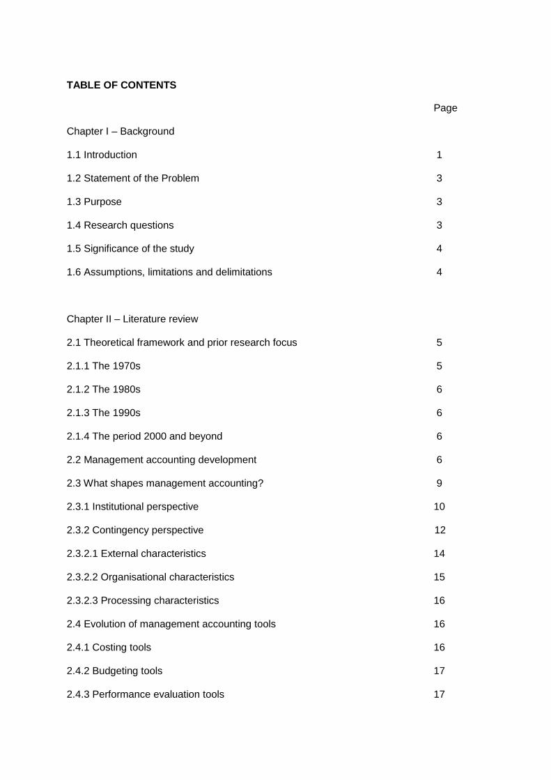
TABLE OF CONTENTS
Page
Chapter I – Background
1.1 Introduction 1
1.2 Statement of the Problem 3
1.3 Purpose 3
1.4 Research questions 3
1.5 Significance of the study 4
1.6 Assumptions, limitations and delimitations 4
Chapter II – Literature review
2.1 Theoretical framework and prior research focus 5
2.1.1 The 1970s 5
2.1.2 The 1980s 6
2.1.3 The 1990s 6
2.1.4 The period 2000 and beyond 6
2.2 Management accounting development 6
2.3 What shapes management accounting? 9
2.3.1 Institutional perspective 10
2.3.2 Contingency perspective 12
2.3.2.1 External characteristics 14
2.3.2.2 Organisational characteristics 15
2.3.2.3 Processing characteristics 16
2.4 Evolution of management accounting tools 16
2.4.1 Costing tools 16
2.4.2 Budgeting tools 17
2.4.3 Performance evaluation tools 17
2.4.4 Profitability analysis tools 17
2.4.5 Investment decision making tools 18
2.4.6 Strategic management accounting tools 18
Chapter III - Methodology
3.1 Population and sample 19
3.2 Instruments 19
3.3 Model and data analysis 20
3.3.1 Usage of tools 21
3.3.2 Importance of tools 21
3.3.3 Contingent factors 21
3.4 Validity, reliability and non-response bias 23
Chapter IV – Results
4.1 Introduction 25
4.2 Results analysis 25
4.3 The contingent factors 26
4.4 Costing tools 28
4.4.1 Costing tools usage 28
4.4.2 Costing tools importance 28
4.4.3 Contingent factors affecting use of costing tools 29
4.5 Budgeting tools 32
4.5.1 Budgeting tools usage 33
4.5.2 Budgeting tools importance 33
4.5.3 Factors affecting use of budgeting tools 34
4.6 Performance evaluation tools 37
4.6.1 Performance evaluation tools usage 38
4.6.2 Performance evaluation tools importance 38
4.6.3 Factors affecting usage of performance evaluation tools 39
4.7 Profitability analysis tools 42
4.7.1 Profitability analysis tools usage 42
4.7.2 Importance of profitability analysis tools 43
4.7.3 Factors influencing usage of profitability analysis tools 43
4.8 Investment decision making tools 45
4.8.1 Investment decision making tools usage 45
4.8.2 Investment decision making tools importance 46
4.8.3 Factors influencing investment decision making tools usage 47
4.9 Strategic management accounting tools 50
4.9.1 Strategic management accounting tools usage 50
4.9.2 Strategic management accounting tools importance 51
4.9.3 Factors influencing SMA tools usage 51
4.10 Summary of ordered probit regression results 54
4.11 Other factors affecting management accounting tools usage 55
4.11.1 Requirements by providers of funds 55
4.11.2 Change in legislation affecting industry 55
4.11.3 Industry practice 55
4.11.4 Head office practice 56
Chapter V Conclusion and recommendations 57
REFERENCES 59
Appendix A – Survey questionnaire 63
Appendix B - independent and dependent variables abbreviations 67
Appendix C - Demographics 69
Appendix D - Ordered Probit regression analysis results 70
Page
List of figures
Figure 1 The Burns and Scapens framework 11
Figure 2 Gordon and Miller’s Framework 13
Figure 3 The Conceptual Model: Factors influencing use of management
accounting tools 14
Figure 4 Costing tools usage 28
Figure 5 Costing tools importance 29
Figure 6 Budgeting tools usage 33
Figure 7 Budgeting tools importance 34
Figure 8 Performance evaluation tools usage 38
Figure 9 Performance evaluation tools importance 39
Figure 10 Profitability analysis tools usage 42
Figure 11 Profitability analysis tools importance 43
Figure 12 Investment decision making tools usage 46
Figure 13 Investment decision making tools importance 47
Figure 14 Strategic management accounting tools usage 50
Figure 15 Strategic management accounting tools importance 51
Page
List of tables
Table 1 Four stages of research focus 5
Table 2 Evolution of the focus of management accounting 8
Table 3 Summary of management accounting tools 20
Table 4 Summary of contingent factors 22
Table 5 Industry sector analysis 26
Table 6 Contingent factor rating 27
Table 7 Probit regression analysis – costing tools 30
Table 8 Probit regression analysis – budgeting tools 35
Table 9 Probit regression analysis – performance evaluation tools 40
Table 10 Probit regression analysis – profitability analysis tools 44
Table 11 Probit regression analysis – investment decision making tools 48
Table 12 Probit regression analysis – SMA tools 53
Table 13 Summary of relationships between factors and tools 54
List of abbreviations
ABB Activity based budgeting
ABC Activity based costing
AICPA Association of International Certified Professional
Accountants
AMT Advanced manufacturing technology
ARR Accounting rate of return
BEP Breakeven point
BSC Balanced scorecard
CIMA Chartered Institute of Management Accountants
DCF Discounted cash flow
IFAC International Federation of Accountants
JIT Just in time
PEU Perceived environmental uncertainty
SMA Strategic management accounting
SWOT Strength, weaknesses, opportunities, threats
TQM Total quality management
1
Chapter I – Background
1.1 Introduction
The increasing level of global competition has intensified the challenges faced by managers.
In response to these challenges a range of new or modern management accounting tools
have been developed to help managers make the right decisions. The new techniques
include activity based costing (ABC), the balanced scorecard (BSC) and strategic
management accounting (SMA) (CIMA, 2013; Drury & Al-Omiria, 2007; Johnson & Kaplan,
1987; Kaplan & Atkinson, 1998). Langfield-Smith and Chenhall (1998) argue that this is the
only way for management accounting to remain relevant in a fast changing business
environment. The new management accounting techniques have been designed to support
modern technologies and new management processes, such as Total Quality Management
(TQM) and Just In Time (JIT) production systems, and to support companies as they try to
achieve a competitive advantage in light of increased global competition (Abdel-Kader &
Luther, 2008).
Business organisations are confronted with several options as to what management
accounting tools would be most effective in responding to their challenging situations (Affes
& Ayad, 2014; Al-Mawali, 2015; Chenhall, 2003). An appropriate mix of management
accounting tools would be one that best suits an organisation’s contextual and operational
contingencies (Chenhall, 2003). Such contingencies include among others, the intensity of
market competition, perceived environmental uncertainty levels, diversity of operations and
technology applied, size and structure of the organisation and type of personnel employed
(Abdel-Kader & Luther, 2006b; Al-Mawali, 2015; Dropulic, 2013; Drury & Al-Omiria, 2007).
There have been limited studies on the application of management accounting tools or
management accounting practices in South Africa (Fakoya, 2014; Waweru, Hoque, & Uliana,
2
2005). There are considerable studies on management accounting practices outside South
Africa (Abdel-Kader & Luther, 2006b; Affes & Ayad, 2014; Ahmad & Leftesi, 2014; Al-
Mawali, 2015; Alleyne & Weeks-Marshal, 2011; Chenhall, 2003; Langfield-Smith & Chenhall,
1998; McNally & Lee, 1980; Montvale, 1994; Sharkar, Sobhan, & Sultana, 2006; Uyar, 2010;
Wijewardena & De Zoysa, 1999; Zabri & Ahmad, 2015). These studies reveal diversity in
management accounting practices between countries and continents, sectors and
organisations and also indicate varying influences of certain contingent factors on the
management accounting tools used.
This study used a questionnaire survey to investigate management accounting tools used by
South African companies. The study further explored the contingent factors that influence
the choice of the management accounting tools employed. These included costing tools,
budgeting tools, performance evaluation tools, profitability analysis tools, investment
decision making tools and strategic management accounting tools. Understanding
management accounting practices and the contingent factors that shape them can assist in
ensuring that management accounting remains relevant and that it continues to add value to
businesses. In their quest to ensure that management accounting remains relevant and
continues to add value the American Institute of Certified Professional Accountants (AICPA)
and the Chartered Institute of Management Accountants (CIMA) who jointly formed the
Association of International Certified Professional Accountants (AICPA) in 2017 prepared
global management accounting principles. The purpose of the principles was to improve
decision-making in organisations through the provision of high quality management
information and to support organisations in benchmarking against best practice (AICPA,
2017). The present article contributes on the importance attributed to management
accounting tools and how these tools are currently supporting organisations in South Africa.
3
1.2 Statement of the Problem
Globalisation has opened up the local market to international players hence there is need for
local companies to adopt best practices if they are to remain competitive. Management
accounting practices adopted by South African companies can affect their ability to compete
on both the international and domestic arena. The quality of information used for decision
making (e.g. on pricing) by South African companies will to a large extent depend on the
level of sophistication of the management accounting tools used. It is therefore important to
know to what extent South African companies use the range of management accounting
tools available and whether they are deriving value from these tools.
1.3 Purpose
The goal of this study was to establish the extent to which management accounting tools are
used by South African companies. In addition, the research sought to gain an understanding
of the factors influencing the use of the management accounting tools by South African
companies. Added to this, it will be beneficial for managers to understand the specific
challenges facing companies in South Africa and how these challenges are affecting the
adoption of the various tools. Finally, the research aimed to give recommendations on future
research regarding management accounting practices in South Africa.
1.4 Research questions
The following research questions were addressed in the study
(i) What management accounting tools are employed by South African companies?
(ii) What level of importance is attached to the various management accounting tools?
(iii) What contingent factors explain the use of the various management accounting
tools?
4
1.5 Significance of the study
The study contributes to the limited academic literature on the use of management
accounting tools or practices in South Africa. By investigating the factors that influence
management accounting practices, the research also fills the research gap in management
accounting literature and provides a basis for further research into management accounting
practices.
The research aims to provide insights that could be used by tertiary institutions and
accounting bodies (such as the Chartered Institute of Management Accountants (CIMA) and
South Africa Institute of Chartered Accountants (SAICA)) on changing industrial needs that
will be valuable for future curricula development. Practitioners will benefit from
understanding what shapes practice and how they can manage change.
1.6 Assumptions, limitations and delimitations
The research assumed that the respondents’ understanding of the questions asked in the
questionnaire were in line with that of the researcher, as the reliability of the survey assumes
consistency in their responses. In addition the study assumed that respondents answered
the questions objectively.
The survey drew responses from companies that were members of the Johannesburg
Chamber of Commerce and Industry (JCCI). One of the limitations of the study is that it only
drew responses from Johannesburg based companies. Secondly the respondents were not
industry specific hence there is scope for further research to identify how specific sectors
may be utilising management accounting tools, as sector specific characteristics have not
been captured in the analysis carried out.
5
Chapter II – Literature Review
2.1 Theoretical framework and prior research focus
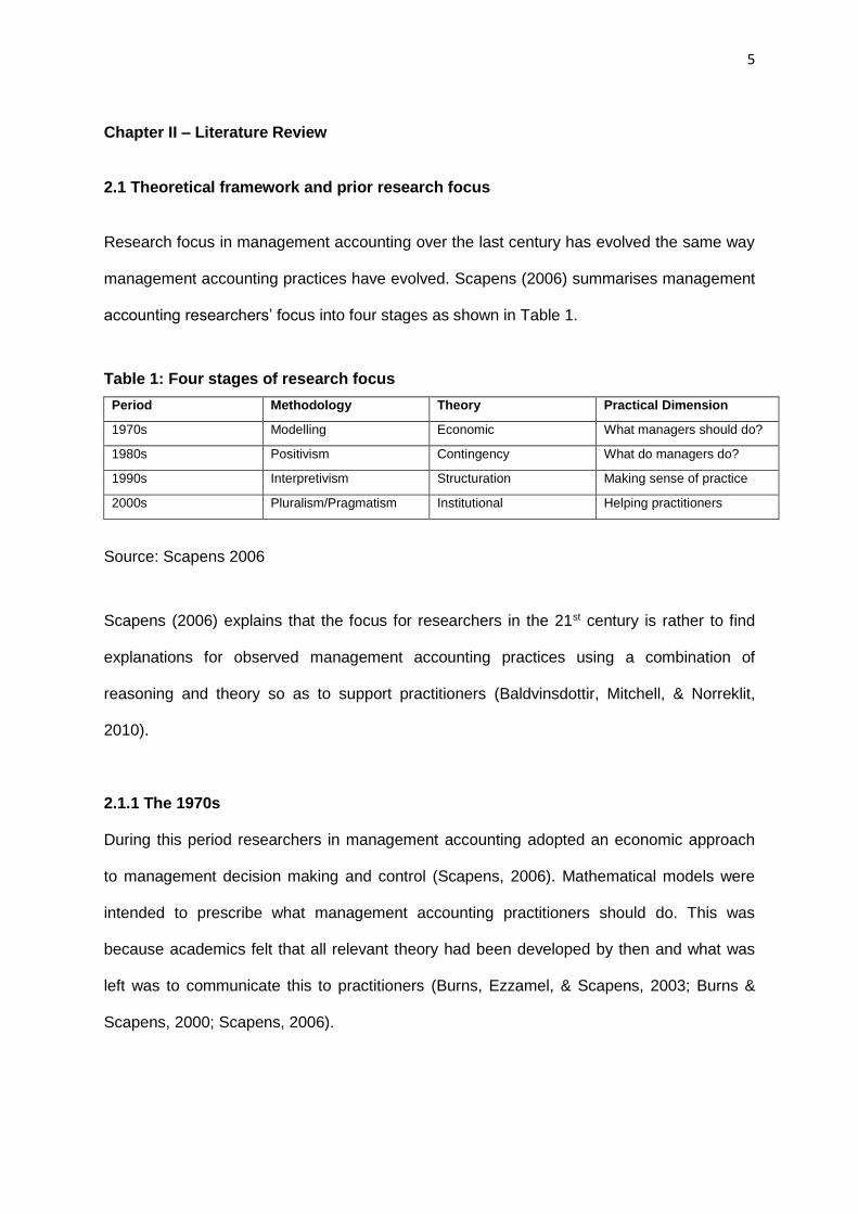
Research focus in management accounting over the last century has evolved the same way
management accounting practices have evolved. Scapens (2006) summarises management
accounting researchers’ focus into four stages as shown in Table 1.
Table 1: Four stages of research focus
Period Methodology Theory Practical Dimension
1970s Modelling Economic What managers should do?
1980s Positivism Contingency What do managers do?
1990s Interpretivism Structuration Making sense of practice
2000s Pluralism/Pragmatism Institutional Helping practitioners
Source: Scapens 2006
Scapens (2006) explains that the focus for researchers in the 21st century is rather to find
explanations for observed management accounting practices using a combination of
reasoning and theory so as to support practitioners (Baldvinsdottir, Mitchell, & Norreklit,
2010).
2.1.1 The 1970s
During this period researchers in management accounting adopted an economic approach
to management decision making and control (Scapens, 2006). Mathematical models were
intended to prescribe what management accounting practitioners should do. This was
because academics felt that all relevant theory had been developed by then and what was
left was to communicate this to practitioners (Burns, Ezzamel, & Scapens, 2003; Burns &
Scapens, 2000; Scapens, 2006).
6
2.1.2 The 1980s
Scapens (2006) claims it became apparent in the 1980s that researchers had limited
knowledge of prevailing management accounting practices. This led researchers to begin
conducting fieldwork interviewing both managers and management accountants and
conducting in-depth longitudinal case studies aimed at establishing what managers do in
practice.
2.1.3 The 1990s
Due to the diversity of management accounting practices observed in the late 1980s and
early 1990s, the focus for management accounting research was to understand why such
diversity in management accounting practice existed (Scapens, 2006). Focus changed from
comparing management accounting practices with conventional prescriptions of economic
theory in order to make sense out of the management accounting practices (Scapens, 1994,
2006).
2.1.4 The period 2000 and beyond
Research focus shifted to try to understand management accounting change in light of
introduction of new advanced management accounting techniques (Robalo, 2014; Scapens,
1994, 2006). Scapens (2006) focused a lot on longitudinal case studies to explore
management accounting change in specific organisations. Research has now taken a
multidisciplinary approach with considerable theoretical diversity, with researchers drawing
on disciplines as wide ranging as economics, organisation theory, sociology, social theory,
politics and anthropology (Burns et al., 2003; Burns & Scapens, 2000; Scapens, 2006).
Many different theoretical approaches such as economic theory, contingency theory and
institutional theory are being applied (Burns et al., 2003; Scapens, 2006).
7
2.2 Management accounting development
In order to understand the application of management accounting tools in any organisation
or country, it is imperative to understand management accounting development and what
shapes management accounting practices (Abdel-Kader & Luther, 2006b; Burns & Vaivio,
2001; Ittner & Larcker, 1998). Kaplan (1984) claimed that virtually all management
accounting practices employed by firms today, and explicated in leading cost accounting
textbooks, had been developed by 1925 and that there has been little innovation in the
design and implementation of cost accounting and management control systems.
There are several reasons why early management accounting practices have been criticised
(Johnson & Kaplan, 1987). Management accounting was perceived to have lost relevance
as it did not meet the needs of contemporary manufacturing and competitive environments.
It focused almost entirely on internal activities with little attention given to external business
environments and as such it had become subservient to financial accounting requirements
(Kaplan, 1984).
Since then, management accounting has gone through a lot of change with the introduction
of new techniques such as activity based costing (ABC), activity based budgeting (ABB),
strategic management accounting (SMA) and the balanced scorecard (BSC) (CIMA, 2009;
Kaplan & Atkinson, 1998).
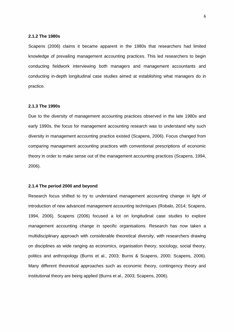
The International Federation of Accountants (IFAC) issued a statement in 1998 describing
developments in management accounting. The federation identified four sequential stages
through which management accounting has developed. The stages are shown in Table 2. It
is imperative to understand these stages of development in this study as there is a link
between the stage of development and the management accounting tools applied by an
entity, industry sector or country (Abdel-Kader & Luther, 2006b).
8
Table 2: Evolution of the focus of Management Accounting
Stage 1 Stage 2 Stage 3 Stage 4
Cost determination
and financial
control
Provision of
information for
management
planning and
control
Reduction of
resource waste
in business
processes
Creation of
value through
effective
resource use
Source: Adopted and modified from IFAC (1998)
Stage 1 - Cost determination and financial control. According to IFAC this stage
represents the period prior to 1950. Focus of management accounting during this era was
determination of product cost through the use of labour hours. Manufacturing processes
were relatively simple and there was not much competition on the products market.
Management was primarily focused on internal matters especially production capacity.
Traditional management accounting tools dominated this era (Askrany, 2005; IFAC, 1998).
Stage 2 – Provision of information for management planning and control. Attention
between the period 1950-1965 was shifted to the provision of information for planning and
control purposes. IFAC sees this as management activity but in a staff role. It involved
support to line management through the use of such technologies, decision analysis and
responsibility accounting. Management accounting as part of management control systems
tended to be reactive, identifying problems and action only when deviations from plans took
place (Abdel-Kader & Luther, 2006a, 2006b; IFAC, 1998).
Stage 3 – Reduction of resource waste in business processes. This was brought about
by the world recession in the 1970s and increased competition underpinned by a rapid
technological development which affected many aspects of the industrial sector.
Developments in computers meant that managers could access and process large amounts
9
of data. The design, maintenance and interpretation of information systems became of
considerable importance in effective management. This challenge of global competition was
met by introducing new management and production techniques and at the same time
controlling costs often through reduction of waste in resources used (IFAC, 1998).
Management accountants were challenged to provide required information through the use
of process analysis and cost management technologies that ensured appropriate information
was available to support managers and employees at all levels (IFAC, 1998).
Stage 4 – Creation of value through effective resources use. As the world-wide industry
faced considerable uncertainty and unprecedented advances in manufacturing and
information processing technologies in the 1990s there was need for management
accountants to focus on creation of value through effective use of resources using
technologies which examine the drivers of customer value, shareholder value and
organisational innovation. The AICPA as the leading professional body for management
accountants is focusing its research on how management accounting can continue to create
value for business in a Volatile, Uncertain, Complex and Ambiguous (VUCA) environment.
Its focus is on how management accountants will remain relevant in an environment where
artificial intelligence and block chain technology are taking over (AICPA, 2017; CIMA, 2009,
2013).
2.3 What shapes management accounting?
Prior studies on what shapes management accounting have taken both contingency
(Chenhall, 2003; Dropulic, 2013) and institutional approaches (Scapens, 2006) to try explain
how management accounting practices evolve over time.
10
2.3.1 The institutional perspective
Adopting an institutional approach to understanding how organisations shape management
accounting practices and how practices in turn shape organisations, Scapens (2006) splits
this institutionalisation into three categories to help explain observed management
accounting practices (Robalo, 2014; Wanderley, Miranda, De Meira, & Cullen, 2011). These
are New Institutional Economics (NIE), New Institutional Sociology (NIS) and Old
Institutional Economics (OIE). According to Scapens (2006) NIE uses reasoning to explain
the diversity in form of institutional arrangements for example differences in markets,
hierarchies and structures (Abdel-Kader & Luther, 2006b; Drury & Tayles, 1994; Kaplan,
1984). Scapens (2006) concluded that NIE draws attention to the economic factors which
help shape the structure of organisations and their management accounting practices
thereby helping understand certain aspects of the mish-mash of interrelated influences.
There is need to look beyond economics to get a fuller understanding of management
accounting practices (Scapens, 2006). New Institutional Economics seeks to explain how
organisations seek to legitimise their existence by conforming to certain standards or
practices so as to be able to secure resources they need for their continued survival
(DiMaggio & Powell, 1983). Such conformance has been classified into different types of
isomorphism – coercive, mimetic and normative. Coercive isomorphism occurs due to
political regulative influences (Fakoya, 2014). Mimetic isomorphism occurs when
organisations seek to copy the practices of other successful organisations and normative
isomorphism is when the norms of society and professional bodies influence the practices of
organisations (Scapens, 2006).
While NIE and NIS help explain the external environment influence on organisations,
Scapens (2006) argues that not all organisations will conform to such pressures and some
may be more susceptible to certain pressures rather than to others. This calls for
researchers to look within organisations so as to understand management accounting
11
practices of individual organisations (Robalo, 2014; Scapens, 1994, 2006; Wanderley et al.,
2011). Old institutional economics seeks to explain how management accounting practices
are shaped by circumstances within the organisation itself. It explores the way habits, rules
and routines can structure economic activity and how they evolve through time.
According to Scapens (2006) adopting an OIE perspective management accounting rules
can be viewed as the rules and routines which shape organisational activity and by studying
how rules and routines evolve a better understanding of management accounting change is
achieved. Ultimately understanding management accounting change means current
management accounting tools can be explained and be in a better position to predict future
management accounting tools application (Abdel-Kader & Luther, 2006b).
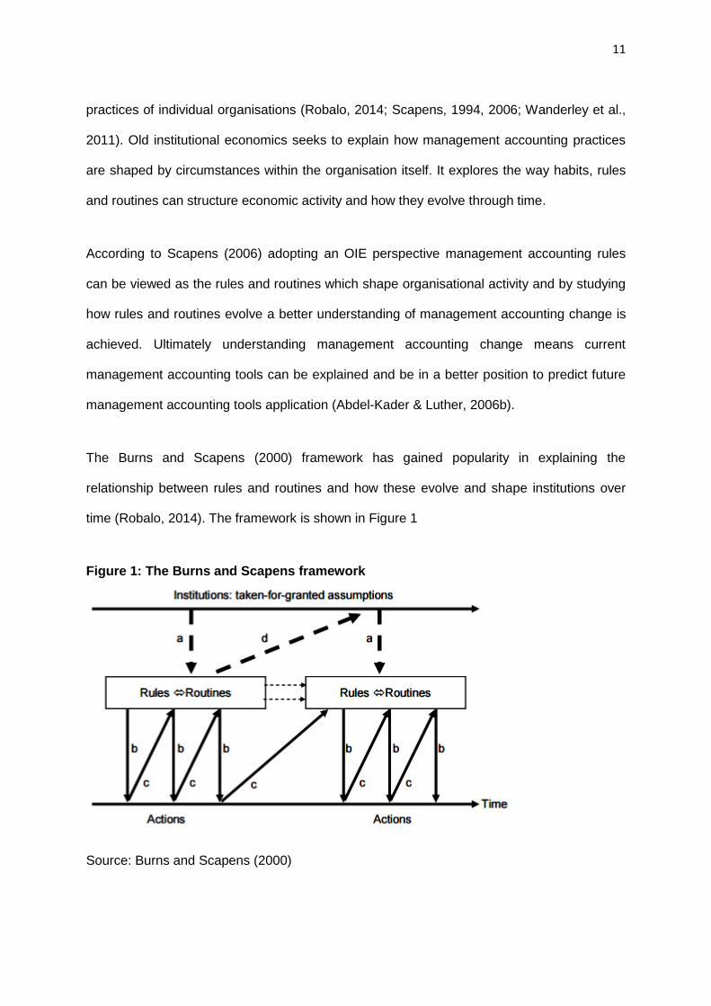
The Burns and Scapens (2000) framework has gained popularity in explaining the
relationship between rules and routines and how these evolve and shape institutions over
time (Robalo, 2014). The framework is shown in Figure 1
Figure 1: The Burns and Scapens framework
Source: Burns and Scapens (2000)
12
According to the Burns and Scapens framework, there is a link between institutions
(institutional realm) and the daily actions carried out by members of the organisation (action
realm). The connection between the two realms is made through rules and routines. The
institutions influence the action at a specific moment in time (synchronised effect), which
explains that the arrows a and b are represented vertically. The actions of the agents
involved in the process of change produce and reproduce institutions over time (diachronic
effect) by way of the creation of routines and rules. This effect of actions on the institutions is
represented through the oblique arrows c and d. The processes of change at the institutional
level require longer periods of time than the processes of change at the level of action;
therefore, the slope of arrow d is not as steep as that of arrow c. This framework shows
management accounting as a set of rules and routines that can be routinised and
institutionalised in organisations. While the framework explains how management
accounting practices develop and change, the framework has been criticised for only paying
attention to organisational internal circumstances (Robalo, 2014; Scapens, 2006).
Scapens (2006) explains that the importance of routinisation and institutionalisation in
explaining management accounting practices cannot be underestimated. Company policy is
entrenched in such history. He used the anecdote of monkeys to explain why practitioners in
some organisations only know how it is done and not why it is done the way they do.
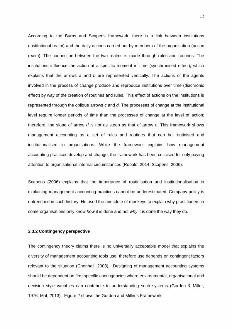
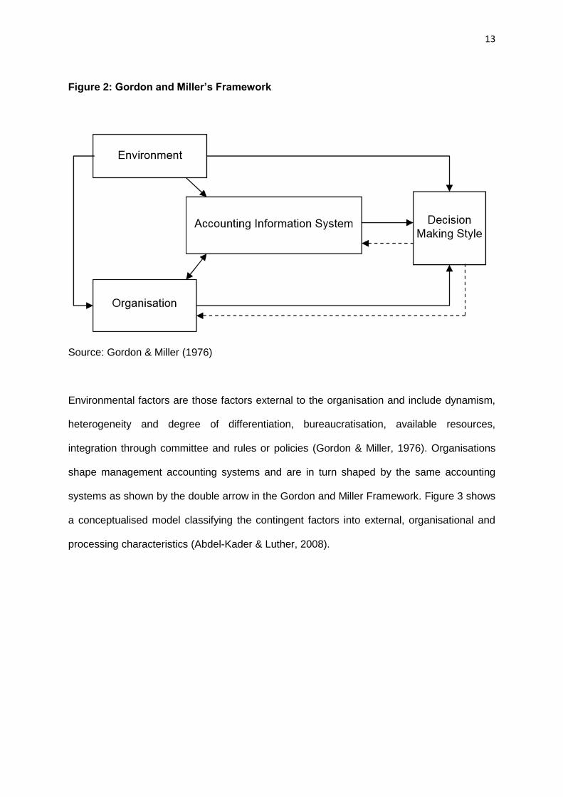
2.3.2 Contingency perspective
The contingency theory claims there is no universally acceptable model that explains the
diversity of management accounting tools use; therefore use depends on contingent factors
relevant to the situation (Chenhall, 2003). Designing of management accounting systems
should be dependent on firm specific contingencies where environmental, organisational and
decision style variables can contribute to understanding such systems (Gordon & Miller,
1976; Mat, 2013). Figure 2 shows the Gordon and Miller’s Framework.
13
Figure 2: Gordon and Miller’s Framework
Source: Gordon & Miller (1976)
Environmental factors are those factors external to the organisation and include dynamism,
heterogeneity and degree of differentiation, bureaucratisation, available resources,
integration through committee and rules or policies (Gordon & Miller, 1976). Organisations
shape management accounting systems and are in turn shaped by the same accounting
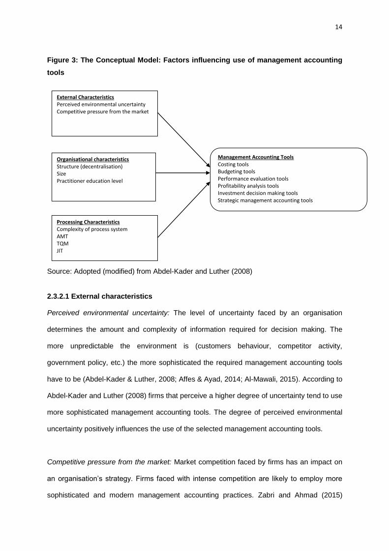
systems as shown by the double arrow in the Gordon and Miller Framework. Figure 3 shows
a conceptualised model classifying the contingent factors into external, organisational and
processing characteristics (Abdel-Kader & Luther, 2008).
14
Figure 3: The Conceptual Model: Factors influencing use of management accounting
tools
Source: Adopted (modified) from Abdel-Kader and Luther (2008)
2.3.2.1 External characteristics
Perceived environmental uncertainty: The level of uncertainty faced by an organisation
determines the amount and complexity of information required for decision making. The
more unpredictable the environment is (customers behaviour, competitor activity,
government policy, etc.) the more sophisticated the required management accounting tools
have to be (Abdel-Kader & Luther, 2008; Affes & Ayad, 2014; Al-Mawali, 2015). According to
Abdel-Kader and Luther (2008) firms that perceive a higher degree of uncertainty tend to use
more sophisticated management accounting tools. The degree of perceived environmental
uncertainty positively influences the use of the selected management accounting tools.
Competitive pressure from the market: Market competition faced by firms has an impact on
an organisation’s strategy. Firms faced with intense competition are likely to employ more
sophisticated and modern management accounting practices. Zabri and Ahmad (2015)
External Characteristics Perceived environmental uncertainty Competitive pressure from the market
Organisational characteristics Structure (decentralisation) Size Practitioner education level
Processing Characteristics Complexity of process system AMT TQM JIT
Management Accounting Tools Costing tools Budgeting tools Performance evaluation tools Profitability analysis tools Investment decision making tools Strategic management accounting tools
15
found a positive relationship between the intensity of market competition and the use of
certain management accounting tools. Competitive pressure from the market has a positive
influence on the use of the selected management accounting tools.
2.3.2.2 Organisational characteristics
Structure (decentralisation): Large and decentralised organisations are characterised by use
of more administrative controls and sophisticated management accounting practices
(Chenhall, 2003). There is need for provision of integrated information hence such
organisations are likely to employ sophisticated management accounting tools. The structure
of an organisation has a positive influence on the application of the selected management
accounting tools.
Size: The size of a firm can be measured by turnover, number of employees or total assets
(Abdel-Kader & Luther, 2008). Larger firms are likely to have adequate resources to support
sophisticated processes and management accounting tools as opposed to smaller
organisations (Abdel-Kader & Luther, 2008; Affes & Ayad, 2014; Chenhall, 2003; Zabri &
Ahmad, 2015). The size of an organisation has a positive influence on the application of the
selected management accounting tools.
Practitioner education level: The level of knowledge that management accountants possess
is likely to have an impact on the complexity of management accounting tools applied.
Practitioners are usually comfortable applying concepts that they are well versed with and
have learnt in their formal studies (Fakoya, 2014; Garg, Ghosh, Hudick, & Nowacki, 2003;
Graham & Harvey, 2001). This study tests whether the practitioner’s level of education has a
positive influence on the application of the selected management accounting tools.
16
2.3.2.3 Processing characteristics
Complexity of process system, technology, total quality management and just-in-time:
Measured by product line diversity, application of advanced manufacturing technology
(AMT), manufacturing resource planning (MRP), computer aided design (CAD), numerical
control (NC), flexible manufacturing systems (FMS) and computer aided inspection, will
impact on the level of management control systems (which management accounting is part
of) (Chenhall, 2003). Previous studies have found that the use of technology had significant
influence on the use of certain management accounting practices (Abdel-Kader & Luther,
2008; Drury & Al-Omiria, 2007; Garg et al., 2003; Sharkar et al., 2006; Wijewardena & De
Zoysa, 1999; Zabri & Ahmad, 2015).
2.4 Evolution of management accounting tools
The last century has seen an unprecedented change in management accounting techniques
with some being introduced as solutions to shortcomings of traditional or contemporary
management accounting tools (Albright & Lam, 2006; Kaplan & Atkinson, 1998).
2.4.1 Costing tools
The focus of costing has changed from mere cost determination and cost classification and
taken a broader view of cost control. Traditionally costing focused on determining product
costs for pricing purposes using some arbitrary methods (Drury & Al-Omiria, 2007; Kaplan &
Cooper, 1998). Costs were mainly classified into variable and fixed (sometimes called
period costs). The increase in competition and demand for accurate product costs has led to
the development of modern costing techniques such as ABC and target costing. This has
been assisted by the improvement in technology which has made processing of volumes of
information faster and easier (Kaplan, 1984; Kaplan & Atkinson, 1998; Sharaf - Addin, Omar,
& Sulaiman, 2014).
17
2.4.2 Budgeting tools
Traditionally budgets were used as benchmark against which success or failure was
measured in terms of resource utilisation over a period. Budgeting horizons tended to be
longer as environments were stable and more predictable. As the business environment
became less predictable and more complex, there was need for new techniques to be
introduced to ensure relevance of the budgets (CIMA, 2013). Budgeting then evolved from
taking a period and incremental approach to using new techniques such as ABB, zero based
budgeting, flexible budgeting and budgeting with what if analysis (CIMA, 2009; Kaplan &
Atkinson, 1998).
2.4.3 Performance evaluation tools
Performance evaluation has traditionally focused on financial measures. Increased
competition has pushed organisations to look at non-financial measures of performance
such as non-financial measures related to customers, employees and operations and
innovation (Ittner & Larcker, 1998; Jinga & Dumitru, 2015). Benchmarking has also been
introduced as a modern technique as organisations try to gain that competitive advantage
(CIMA, 2013).
2.4.4 Profitability analysis tools
Improvements in costing techniques have resulted in better profitability measures being
introduced. The ability to establish product costs using ABC has meant that organisations
could shift from looking at overall organisational profitability and focus on product or
customer profitability (CIMA, 2013; Sharaf - Addin et al., 2014). Improvements in technology
have also assisted in coming up with sophisticated and efficient stock models.
18
2.4.5 Investment decision making tools
The payback method used to be the most popular method of evaluating capital projects
(Graham & Harvey, 2001; Kaplan & Atkinson, 1998). In a VUCA world the variables on
capital projects become so complicated that the payback period is faced with a lot of
inadequacies. As a result, modern capital appraisal techniques that take into account the risk
profile of cash flows have been developed. These include discounted cash flow methods and
computer simulation (Graham & Harvey, 2001). The 21st century has seen an increase in
pressure from environmental activists which has brought another dimension to investment
appraisal. Organisations are now being forced to include the social impact of their projects in
their investment appraisals (Graham & Harvey, 2001; Jinga & Dumitru, 2015).
2.4.6 Strategic management accounting tools
Strategic management accounting is a fairly new concept in management accounting. SMA
tools have been developed in an attempt to ensure management accounting remains
relevant (CIMA, 2013; Roslender, 1996). The VUCA world entails that organisations must
pay more attention to external factors now than before as they craft their strategies (AICPA,
2017; CIMA, 2013). The range of SMA tools includes forecasting, shareholder value
analysis, industry analysis, competitor position analysis, value chain analysis and strength,
weaknesses, opportunities and threats (SWOT) analysis (Kaplan & Atkinson, 1998;
Langfield-Smith & Chenhall, 1998).
This chapter has reviewed how management accounting practices have evolved over time
using both an institutional and a contingent perspective. Contingent factors that influence
management accounting tools usage have been explored. Selected management
accounting tools have also been explained. This study focuses on how the contingent factors
influence usage of the selected management accounting tools in the South African context.
19
Chapter III – Methodology
3.1 Population and Sample
The research used a positivist approach in testing the following three research questions.
RQ1: What management accounting tools are employed by South African companies?
RQ2: What level of importance is attached to the various management accounting tools?
RQ3: What contingent factors explain the use of the various management accounting tools
in the South African context? The data collection aimed at gathering data on management
accounting tools usage, their importance to firms in the South African context and the
possible factors influencing their application. A survey questionnaire was used to collect the
required data.
For the purpose of this study the population was defined as all firms in South Africa. The
sample was drawn from firms registered with the Johannesburg Chamber of Commerce and
Industry (JCCI) as at 30 September 2016. The researcher obtained a database with 1332
members. Of these 1 142 had telephone numbers and only 995 had email addresses.
3.2 Instruments
The research was based on a comprehensive online questionnaire (copy included in
Appendix A) designed to collect the required data from respondents. The questionnaire was
designed using Survey Monkey. This questionnaire was modelled along the same
parameters as ones used in prior research (Abdel-Kader & Luther, 2006b, 2008; CIMA,
2009; Zabri & Ahmad, 2015).
Section A of the questionnaire was designed to collect demographic data. In section B
respondents were required to indicate whether they used or did not use the selected
management accounting tools. In addition, respondents were requested to indicate the level
20
of usage or importance on a Likert scale where 1 was not used and 5 was frequently
used/very important signifying the level of importance of each of the 37 management
accounting tools to their organisations. In section C, to ascertain what contingent factors
affected use of the management accounting tools, respondents were required to rate each of
the contingent factors for their organisations. In this section the survey collected data to
determine whether there is a relationship between selected contingent factors and the
selected management accounting tools. Section D of the questionnaire required respondents
to indicate which management accounting tools their organisations would be adopting soon.
The questionnaire ended with a general comments box requesting respondents to give a
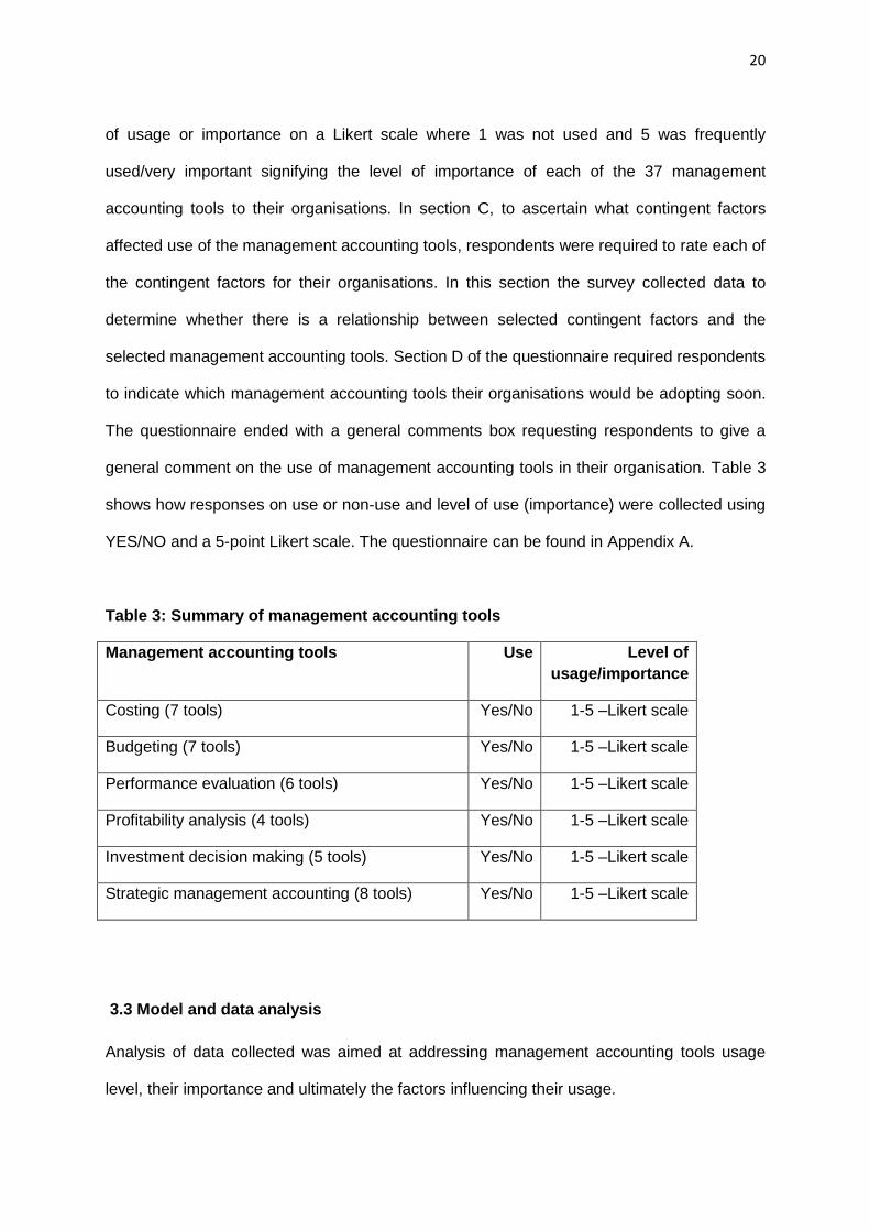
general comment on the use of management accounting tools in their organisation. Table 3
shows how responses on use or non-use and level of use (importance) were collected using
YES/NO and a 5-point Likert scale. The questionnaire can be found in Appendix A.
Table 3: Summary of management accounting tools
Management accounting tools Use Level of
usage/importance
Costing (7 tools) Yes/No 1-5 –Likert scale
Budgeting (7 tools) Yes/No 1-5 –Likert scale
Performance evaluation (6 tools) Yes/No 1-5 –Likert scale
Profitability analysis (4 tools) Yes/No 1-5 –Likert scale
Investment decision making (5 tools) Yes/No 1-5 –Likert scale
Strategic management accounting (8 tools) Yes/No 1-5 –Likert scale
3.3 Model and data analysis
Analysis of data collected was aimed at addressing management accounting tools usage
level, their importance and ultimately the factors influencing their usage.
21
3.3.1 Usage of tools
Data collected on use or non-use of the various tools was analysed using descriptive
statistics. Statistics such as what percentage of the respondents used a tool was calculated
and presented in the form of graphs, charts and tables.
3.3.2 Importance of tools The level of importance of each tool was analysed using descriptive statistics. A
management accounting tool with a rating of 5 means that the tool was very frequently used
or very important for the firm. Calculating the sample mean for each management
accounting tool assisted in rating how important (level of usage) the management
accounting tool was in the sample e.g. a mean of 4 on budgeting would indicate that budgets
are frequently used by the sampled companies. Means and medians were also calculated
and assisted in analysing the data on the level of usage or importance.
3.3.3 Contingent factors Nine contingent factors were tested against each of the 37 management accounting tools to
establish whether the contingent factors influenced the level of importance associated with
each tool. This was done using ordered probit regression analysis. The contingent factors
were the independent variables in the regression model. Table 4 shows a summary of the
factors. Respondents were asked to rank these on a Likert scale of 1-5.
22
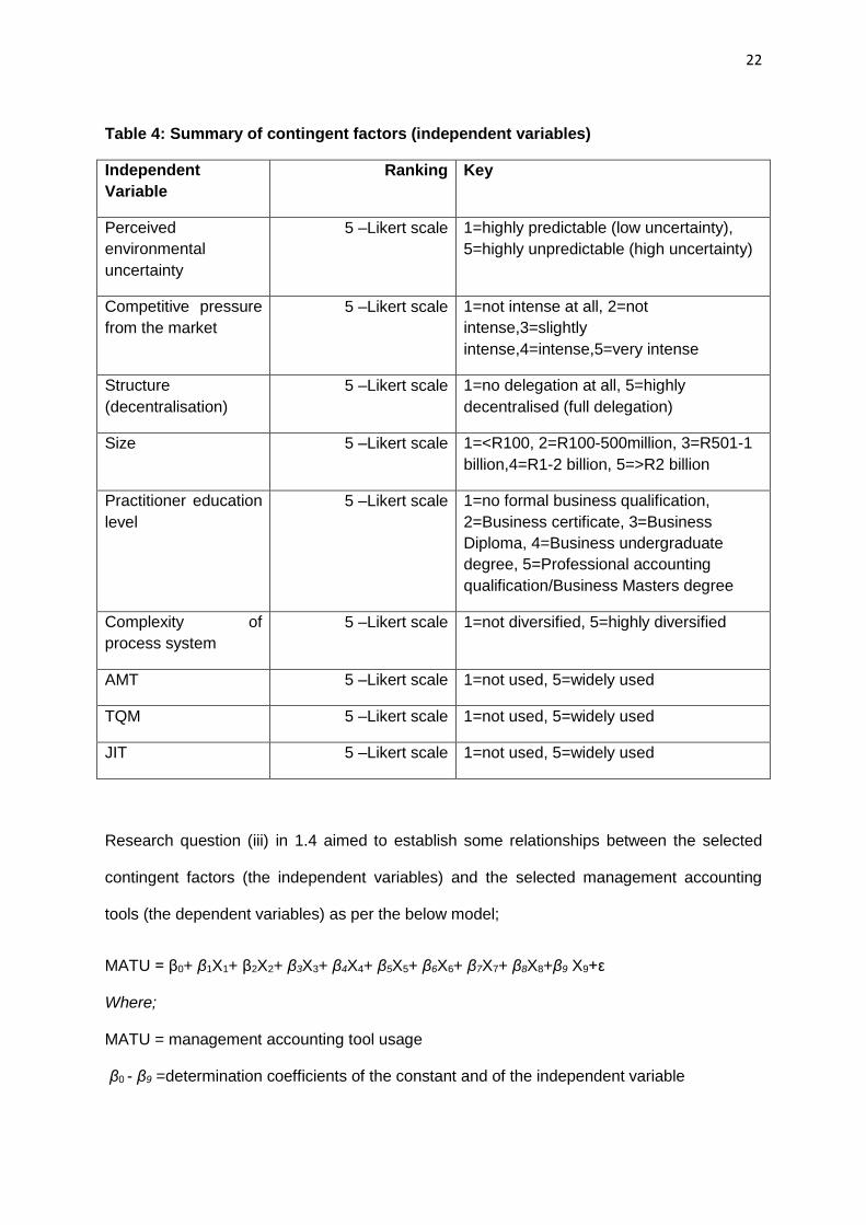
Table 4: Summary of contingent factors (independent variables)
Independent
Variable
Ranking Key
Perceived
environmental
uncertainty
5 –Likert scale 1=highly predictable (low uncertainty),
5=highly unpredictable (high uncertainty)
Competitive pressure
from the market
5 –Likert scale 1=not intense at all, 2=not
intense,3=slightly
intense,4=intense,5=very intense
Structure
(decentralisation)
5 –Likert scale 1=no delegation at all, 5=highly
decentralised (full delegation)
Size 5 –Likert scale 1=<R100, 2=R100-500million, 3=R501-1
billion,4=R1-2 billion, 5=>R2 billion
Practitioner education
level
5 –Likert scale 1=no formal business qualification,
2=Business certificate, 3=Business
Diploma, 4=Business undergraduate
degree, 5=Professional accounting
qualification/Business Masters degree
Complexity of
process system
5 –Likert scale 1=not diversified, 5=highly diversified
AMT 5 –Likert scale 1=not used, 5=widely used
TQM 5 –Likert scale 1=not used, 5=widely used
JIT 5 –Likert scale 1=not used, 5=widely used
Research question (iii) in 1.4 aimed to establish some relationships between the selected
contingent factors (the independent variables) and the selected management accounting
tools (the dependent variables) as per the below model;
MATU = β0+ β1X1+ β2X2+ β3X3+ β4X4+ β5X5+ β6X6+ β7X7+ β8X8+β9 X9+ε
Where;
MATU = management accounting tool usage
β0 - β9 =determination coefficients of the constant and of the independent variable
23
X1-X9 = the contingent factors or independent variables i.e. (perceived environmental
uncertainty, competitive pressure from the market, structure, size, practitioner education
level, complexity of process, AMT, TQM, JIT)
ε = error term
Since the data is ranked and not linear, ordered probit regression analysis was used to test
for the relationship between the contingent factors (independent variable) and management
accounting tool (dependent variable). The researcher used Eview software and Excel for
statistical analysis and data presentation. The model was run 37 times as 37 tools were
assessed. The list of abbreviations used when running the model are in Appendix B. The
results of the statistical analysis are shown in Appendix C.
A positive parameter in the regression model indicates that higher values of the associated
contingent variable (X) increases the probability of the importance of the tool (Y). For
example, a positive contingence factor will increase the probability for a higher ranking on
the importance, ceteris paribus; a negative contingence factor will decrease the probability
for a higher ranking on the importance, ceteris paribus. So only, the sign of the
parameter/coefficient of the results can be interpreted. To interpret the magnitude of the
coefficients the marginal effect has to be calculated. The marginal effect gives the increase
in probability of the importance of the dependent variable for each unit increase of the
independent variable. The coefficients and the marginal effects for the 37 regression models
were calculated and are included in Appendix B.
3.4 Validity, reliability and non-response bias
The questionnaire was piloted prior to being sent to the companies. Following the feedback
received there were some changes to the questionnaire. The statistical analysis was carried
out with the help of a statistician who ensured that the procedures followed were appropriate

24
for use of the Ordered Probit regression model. The researcher is also confident of the
results of the survey as the questionnaires were directed to the Finance Departments to
make sure they were completed by people who understood the subject matter.
25
Chapter IV – Results
4.1 Introduction
The researcher contacted the selected companies by email to alert them of the impending
research questionnaire. Emails targeted CFO/accountants and, where there was no finance
contact, recipients were requested to forward the emails to their finance personnel.
Respondents were given two weeks to respond to the questionnaire. The response rate was
very low with less than 30 responses received in two weeks. The researcher then decided to
follow up by resending the emails for the second time and calling the respondents as a
reminder.
Questionnaires were e-mailed to respondents on the 3rd of January 2017. Respondents had
up to the 17th of January 2017 to complete the questionnaire. The target response rate was
100 usable questionnaires. The researcher however managed to get 66 responses from the
942 targeted respondents signifying a 7% response rate. Of the 66 responses only 38
responses were fully complete; meaning 28 of the questionnaires could not be used for the
purpose of this study. Even though the number of usable questionnaires was low, upon
consulting with the statistician that carried out the analysis it was established that 38
responses would be sufficient to carry out the ordered probit regression.
4.2 Results analysis
The first research question (RQ1) aimed to establish which of the selected management
accounting tools were employed by companies in South Africa. RQ1 is restated here.
RQ1: What management accounting tools are employed by South African companies? The
second research question (RQ2) sought to establish the level of importance attached to
each management accounting tool. The research question is restated here. RQ2: What level
of importance is attached to the various management accounting tools?
26
The difference between the first and second research questions is that RQ2 asks
respondents to rate the importance of each tool to their organisations using a 5-point Likert
scale whereas RQ1 only focused on whether a tool was used or not.
The third research question aimed to establish if there was a relationship between use of
selected management accounting tools and selected contingent factors. The research
question is restated as follows: RQ3 – What contingent factors explain the use of the various
management accounting tools in the South African context? Respondents were asked to
rank the nine contingent factors on a 5-point Likert scale. The results of their ranking are
shown in Table 6.
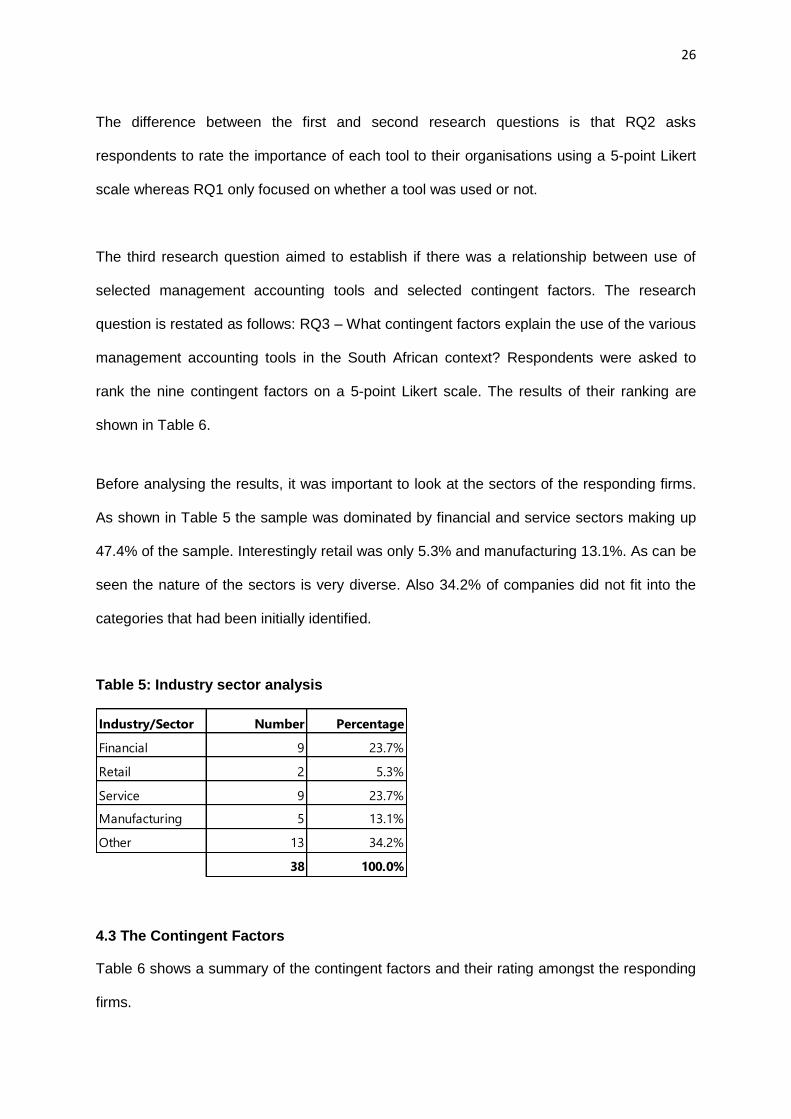
Before analysing the results, it was important to look at the sectors of the responding firms.
As shown in Table 5 the sample was dominated by financial and service sectors making up
47.4% of the sample. Interestingly retail was only 5.3% and manufacturing 13.1%. As can be
seen the nature of the sectors is very diverse. Also 34.2% of companies did not fit into the
categories that had been initially identified.
Table 5: Industry sector analysis
Industry/Sector Number Percentage
Financial 9 23.7%
Retail 2 5.3%
Service 9 23.7%
Manufacturing 5 13.1%
Other 13 34.2%
38 100.0%
4.3 The Contingent Factors
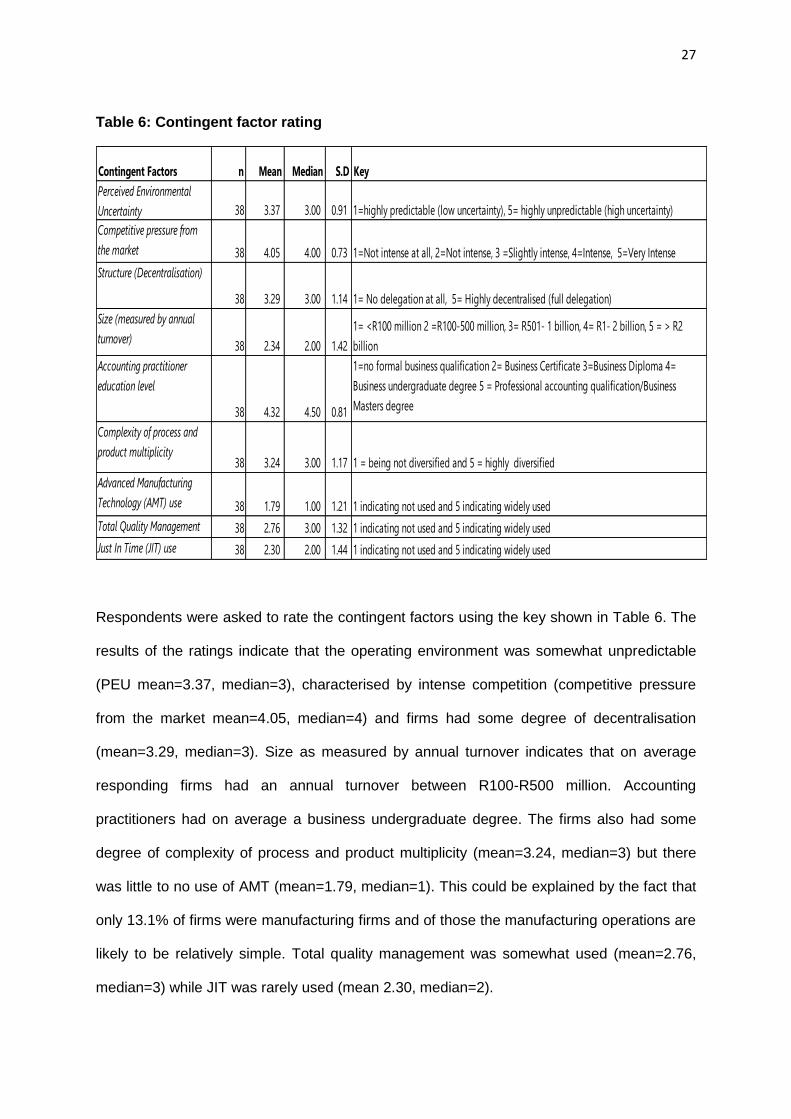
Table 6 shows a summary of the contingent factors and their rating amongst the responding
firms.
27
Table 6: Contingent factor rating
Contingent Factors n Mean Median S.D Key
Perceived Environmental
Uncertainty 38 3.37 3.00 0.91 1=highly predictable (low uncertainty), 5= highly unpredictable (high uncertainty)
Competitive pressure from
the market 38 4.05 4.00 0.73 1=Not intense at all, 2=Not intense, 3 =Slightly intense, 4=Intense, 5=Very Intense
Structure (Decentralisation)
38 3.29 3.00 1.14 1= No delegation at all, 5= Highly decentralised (full delegation)
Size (measured by annual
turnover) 38 2.34 2.00 1.42
1= <R100 million 2 =R100-500 million, 3= R501- 1 billion, 4= R1- 2 billion, 5 = > R2
billion
Accounting practitioner
education level
38 4.32 4.50 0.81
1=no formal business qualification 2= Business Certificate 3=Business Diploma 4=
Business undergraduate degree 5 = Professional accounting qualification/Business
Masters degree
Complexity of process and
product multiplicity38 3.24 3.00 1.17 1 = being not diversified and 5 = highly diversified
Advanced Manufacturing
Technology (AMT) use 38 1.79 1.00 1.21 1 indicating not used and 5 indicating widely used
Total Quality Management
(TQM) use
38 2.76 3.00 1.32 1 indicating not used and 5 indicating widely used
Just In Time (JIT) use 38 2.30 2.00 1.44 1 indicating not used and 5 indicating widely used
Respondents were asked to rate the contingent factors using the key shown in Table 6. The
results of the ratings indicate that the operating environment was somewhat unpredictable
(PEU mean=3.37, median=3), characterised by intense competition (competitive pressure
from the market mean=4.05, median=4) and firms had some degree of decentralisation
(mean=3.29, median=3). Size as measured by annual turnover indicates that on average
responding firms had an annual turnover between R100-R500 million. Accounting
practitioners had on average a business undergraduate degree. The firms also had some
degree of complexity of process and product multiplicity (mean=3.24, median=3) but there
was little to no use of AMT (mean=1.79, median=1). This could be explained by the fact that
only 13.1% of firms were manufacturing firms and of those the manufacturing operations are
likely to be relatively simple. Total quality management was somewhat used (mean=2.76,
median=3) while JIT was rarely used (mean 2.30, median=2).
28
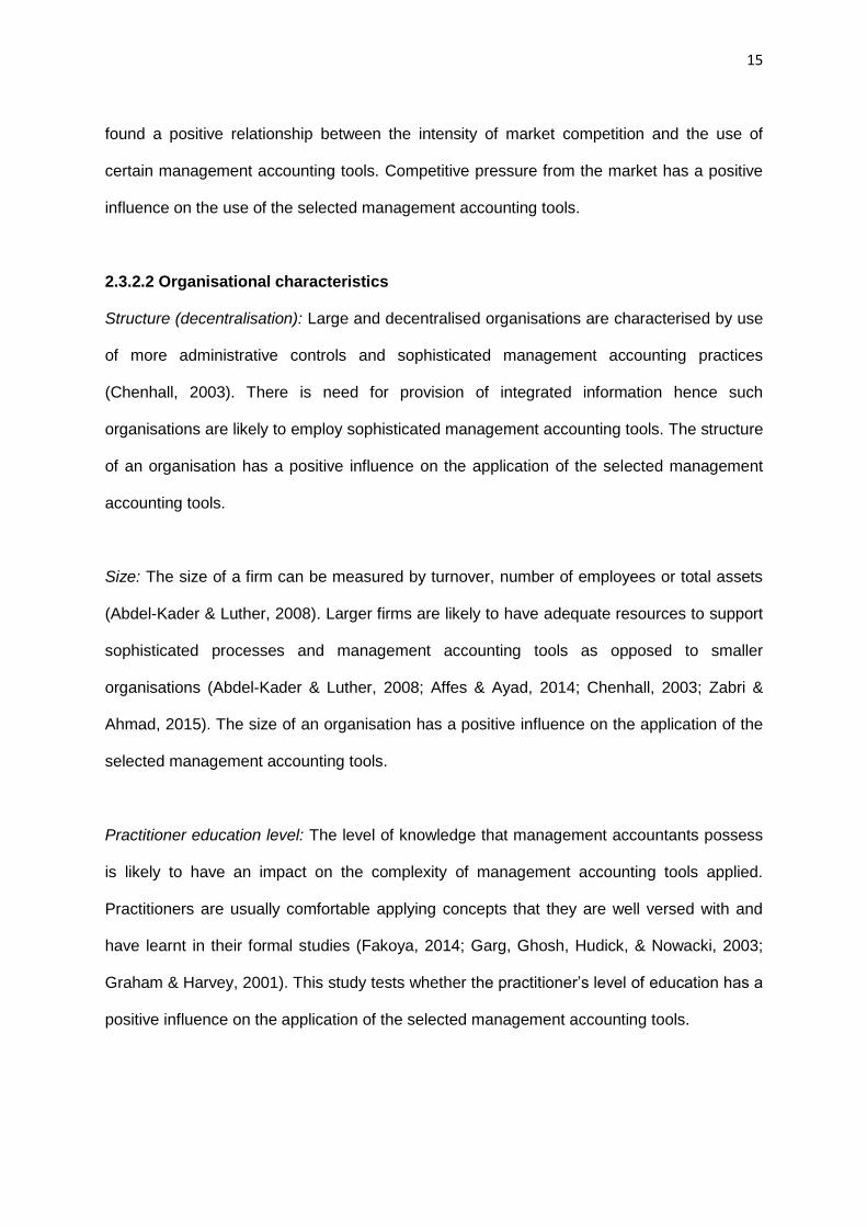
4.4 Costing tools
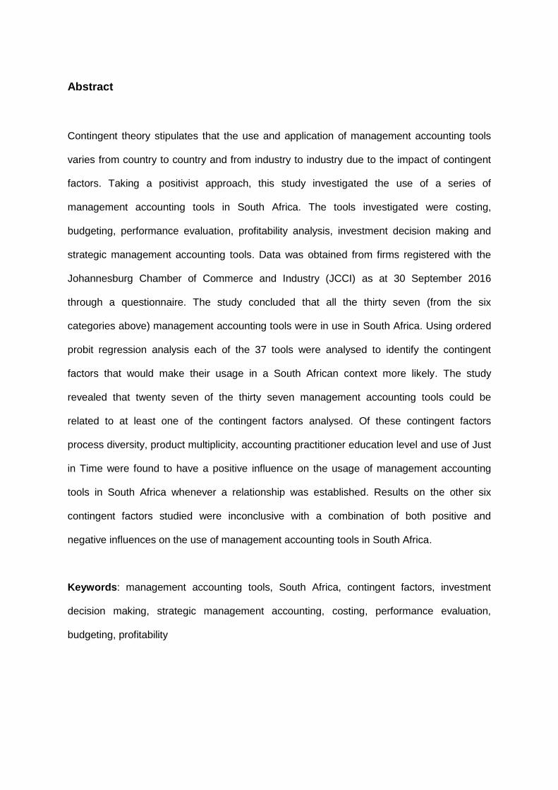
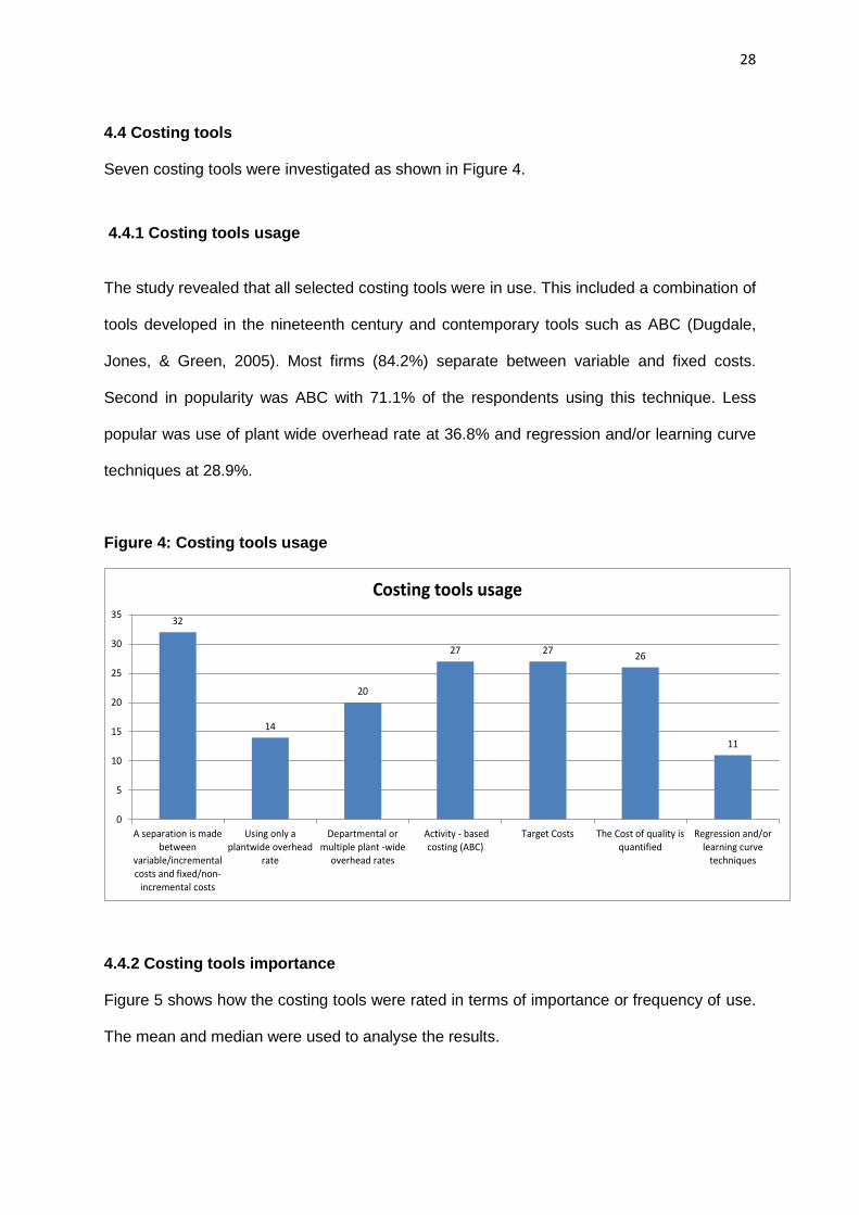
Seven costing tools were investigated as shown in Figure 4.
4.4.1 Costing tools usage
The study revealed that all selected costing tools were in use. This included a combination of
tools developed in the nineteenth century and contemporary tools such as ABC (Dugdale,
Jones, & Green, 2005). Most firms (84.2%) separate between variable and fixed costs.
Second in popularity was ABC with 71.1% of the respondents using this technique. Less
popular was use of plant wide overhead rate at 36.8% and regression and/or learning curve
techniques at 28.9%.
Figure 4: Costing tools usage
32
14
20
27 2726
11
0
5
10
15
20
25
30
35
A separation is madebetween
variable/incrementalcosts and fixed/non-
incremental costs
Using only aplantwide overhead
rate
Departmental ormultiple plant -wide
overhead rates
Activity - basedcosting (ABC)
Target Costs The Cost of quality isquantified
Regression and/orlearning curve
techniques
Costing tools usage
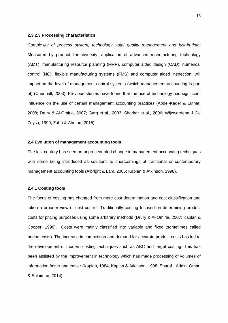
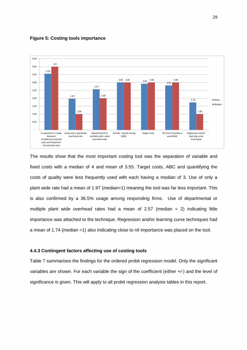
4.4.2 Costing tools importance
Figure 5 shows how the costing tools were rated in terms of importance or frequency of use.
The mean and median were used to analyse the results.
29
Figure 5: Costing tools importance
3.55
1.97
2.57
3.00 2.92
2.81
1.74
4.0
1.00
2.00
3.00 3.00 3.00
1.00
-
0.50
1.00
1.50
2.00
2.50
3.00
3.50
4.00
4.50
A separation is madebetween
variable/incrementalcosts and fixed/non-
incremental costs
Using only a plantwideoverhead rate
Departmental ormultiple plant -wide
overhead rates
Activity - based costing(ABC)
Target Costs The Cost of quality isquantified
Regression and/orlearning curve
techniques
Mean
Median
The results show that the most important costing tool was the separation of variable and
fixed costs with a median of 4 and mean of 3.55. Target costs, ABC and quantifying the
costs of quality were less frequently used with each having a median of 3. Use of only a
plant wide rate had a mean of 1.97 (median=1) meaning the tool was far less important. This
is also confirmed by a 36.5% usage among responding firms. Use of departmental or
multiple plant wide overhead rates had a mean of 2.57 (median = 2) indicating little
importance was attached to the technique. Regression and/or learning curve techniques had
a mean of 1.74 (median =1) also indicating close to nil importance was placed on the tool.
4.4.3 Contingent factors affecting use of costing tools
Table 7 summarises the findings for the ordered probit regression model. Only the significant
variables are shown. For each variable the sign of the coefficient (either +/-) and the level of
significance is given. This will apply to all probit regression analysis tables in this report.
30
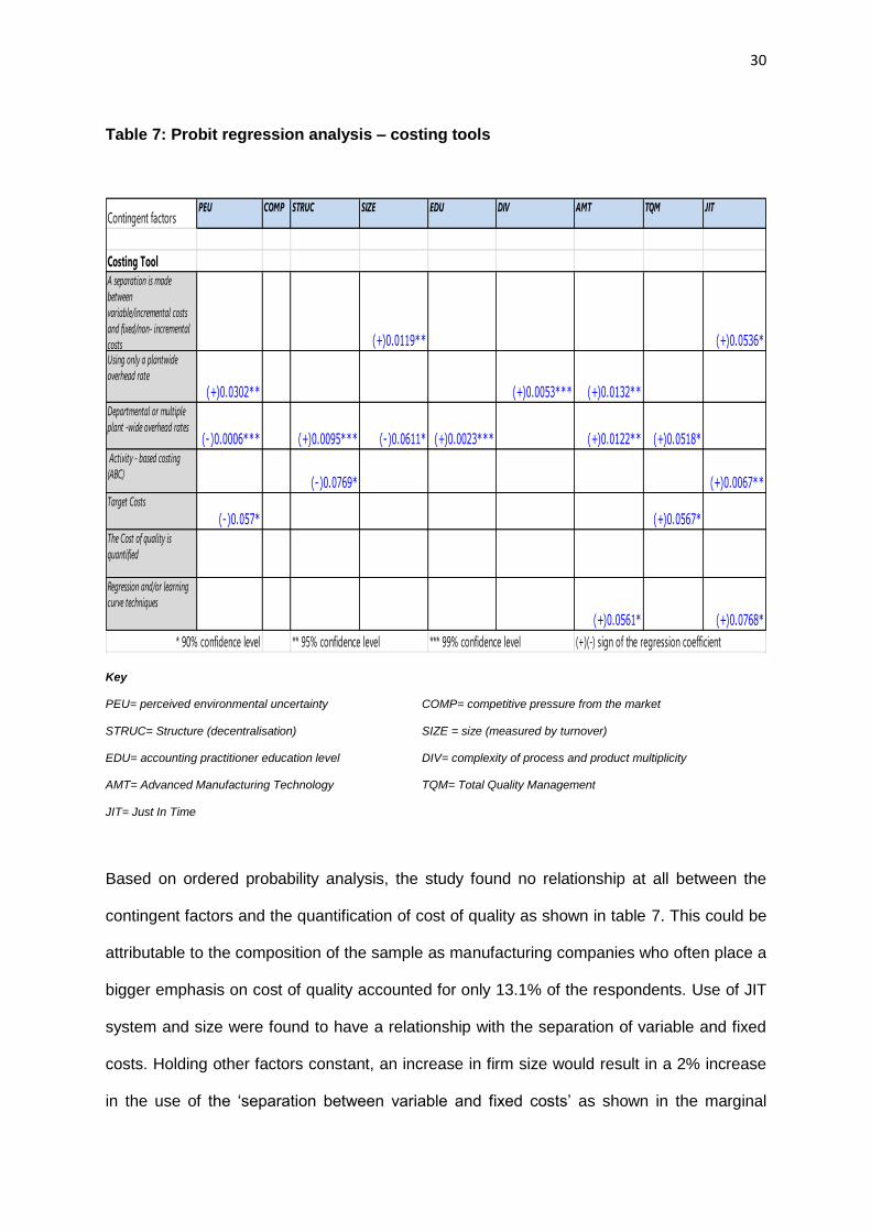
Table 7: Probit regression analysis – costing tools
Contingent factorsPEU COMP STRUC SIZE EDU DIV AMT TQM JIT
Costing Tool
A separation is made
between
variable/incremental costs
and fixed/non- incremental
costs (+)0.0119** (+)0.0536*
Using only a plantwide
overhead rate
(+)0.0302** (+)0.0053*** (+)0.0132**
Departmental or multiple
plant -wide overhead rates(-)0.0006*** (+)0.0095*** (-)0.0611* (+)0.0023*** (+)0.0122** (+)0.0518*
Activity - based costing
(ABC)(-)0.0769* (+)0.0067**
Target Costs
(-)0.057* (+)0.0567*
The Cost of quality is
quantified
Regression and/or learning
curve techniques
(+)0.0561* (+)0.0768*
* 90% confidence level ** 95% confidence level *** 99% confidence level (+)(-) sign of the regression coefficient
Key
PEU= perceived environmental uncertainty COMP= competitive pressure from the market
STRUC= Structure (decentralisation) SIZE = size (measured by turnover)
EDU= accounting practitioner education level DIV= complexity of process and product multiplicity
AMT= Advanced Manufacturing Technology TQM= Total Quality Management
JIT= Just In Time
Based on ordered probability analysis, the study found no relationship at all between the
contingent factors and the quantification of cost of quality as shown in table 7. This could be
attributable to the composition of the sample as manufacturing companies who often place a
bigger emphasis on cost of quality accounted for only 13.1% of the respondents. Use of JIT
system and size were found to have a relationship with the separation of variable and fixed
costs. Holding other factors constant, an increase in firm size would result in a 2% increase
in the use of the ‘separation between variable and fixed costs’ as shown in the marginal
31
effect (Equation 1, Appendix D). The greater the firm size (turnover) the more likely a
separation of variable and fixed costs is done. A JIT system will increase the probability of a
higher ranking of the separation between variable and fixed costs. All other things being
equal, a unit increase in JIT will result in a 2% increase in the application of the separation
between variable and fixed costs. Use of only plant wide overhead rate could be related to
PEU, complexity of process and product and use of AMT as shown in Table 7. Holding other
factors constant, a unit increase in the PEU would result in a 0.2% increase in the use of
only plant wide overhead rate. As product diversity and process complexity increases there
is only a marginal increase in the use of only plant wide overhead rates. An increase in use
of AMT would also result in a marginal increase in the use of only plant wide overhead rate.
The more diversified the product range and complex the manufacturing process is, the
greater the fixed costs. In such environments there is need to allocate overheads to a variety
of products based not only on plant wide overhead rate (Drury & Al-Omiria, 2007).
The most outstanding tool was the use of departmental or multiple plant overhead rates.
This could be linked to six of the nine contingent factors investigated. A unit increase in PEU
(holding other factors constant) would result in 4% decrease in the use of multiple plant
overhead rates. A unit increase in structure (decentralisation) would result in a 22% increase
in the use of multiple plant overhead rates. This is more common in decentralised
organisations who have to share costs relating to shared services amongst operating
business units (Drury & Tayles, 1994). As the size (measured by turnover) increases the use
of multiple plant wide overhead rates goes down by 10% (see Appendix D).
The study revealed that as the management accounting practitioner’s level of education
increases use of multiple plant wide overhead rates become increasingly prevalent. This
could be attributed to practitioners applying what they learnt in business school, see Graham
and Harvey (2001). According to the results holding other factors constant, a unit increase in
32
practitioner’s education level would result is a 23% increase in the use of multiple plant wide
overhead rates.
Activity based costing could only be linked to structure and JIT usage contrary to prior
studies which established a relation between ABC and all the nine contingent factors (Abdel-
Kader & Luther, 2006b; Drury & Al-Omiria, 2007). This could be attributable to the fact that
there were less manufacturing companies in the sample. According to the results the more
decentralised an organisation is, the less likely the use of ABC as business units become
autonomous.
Target costing could be linked to PEU and TQM. An increase PEU would reduce the
importance of target costing all other factors remaining constant. On the other hand an
increase in the use of TQM would result in an increase in the use of target costing. An
organisation that employs TQM will monitor all its costs and would not accept any deviations
in the cost of their products.
Regression and/or learning curve techniques are complex mathematical models that require
proper systems to be implemented and benefit organisations. According to the study use of
this tool could only be linked to AMT and JIT systems. The lack of sophisticated
manufacturing companies in the sample could also have contributed to the results.
4.5 Budgeting tools
Seven budgeting tools were investigated. These were budgeting for planning, budgeting for
controlling costs, activity based budgeting, budgeting with ‘what if’ analysis, flexible
budgeting, zero based budgeting and budgeting for long term (strategic) plans.
33
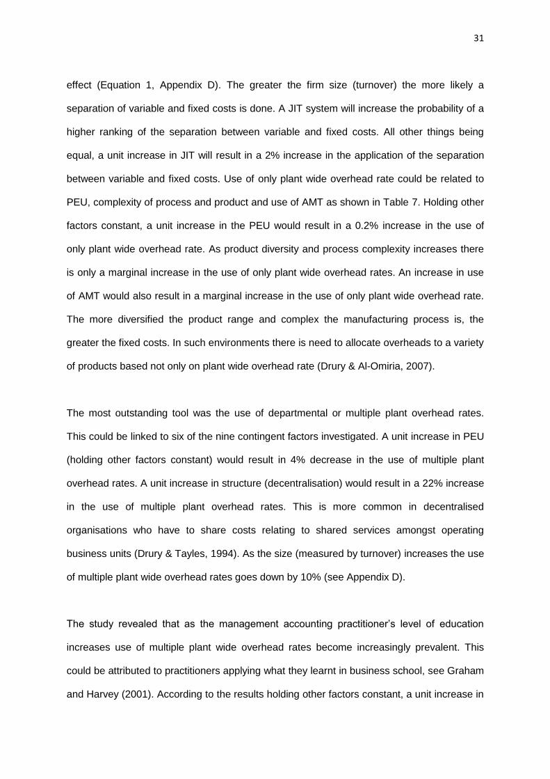
4.5.1 Budgeting tools usage
Budgeting tools appeared to be the most popular with 97.4% of the respondents indicating
using at least one of the selected budgeting tools. ZBB as well as ABB was used by 71.1%
of firms. Ninety seven percent used budgeting for planning and controlling costs. The results
from the analysis are shown in figure 6.
Figure 6: Budgeting tools usage
37 37
2729
31
27
33
0
5
10
15
20
25
30
35
40
Budgeting forplanning
Budgeting forcontrolling
costs
Activity- basedbudgeting
Budgetingwith 'what if
analysis'
Flexiblebudgeting
Zero- basedbudgeting
Budgeting forlong term(strategic)
plans
Budgeting tools usage
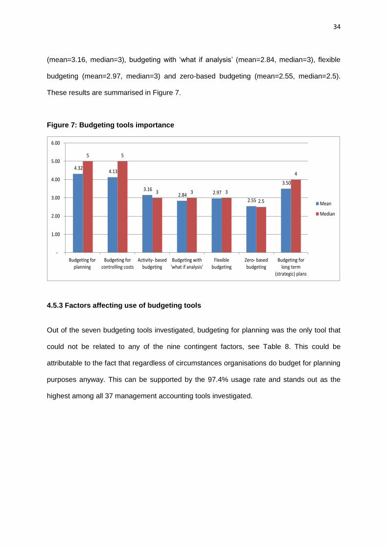
4.5.2 Budgeting tools importance
Budgeting as a management accounting tool received the highest rating in terms of
importance. Budgeting for planning had a mean of 4.33 (median=5) indicating very frequent
use and very high importance. Out of the 38 respondents only one company (2.6%)
confirmed they did not use budgets at all. Budgeting for controlling costs with a mean of 4.13
(median =5) ranked second among budgeting tools. Budgeting for long term (strategic) plans
was third in importance with a mean of 3.5 and median of 4. Less frequently used were ABB
34
(mean=3.16, median=3), budgeting with ‘what if analysis’ (mean=2.84, median=3), flexible
budgeting (mean=2.97, median=3) and zero-based budgeting (mean=2.55, median=2.5).
These results are summarised in Figure 7.
Figure 7: Budgeting tools importance
4.32 4.13
3.16 2.84 2.97
2.55
3.50
5 5
3 3 3
2.5
4
-
1.00
2.00
3.00
4.00
5.00
6.00
Budgeting forplanning
Budgeting forcontrolling costs
Activity- basedbudgeting
Budgeting with'what if analysis'
Flexiblebudgeting
Zero- basedbudgeting
Budgeting forlong term
(strategic) plans
Mean
Median
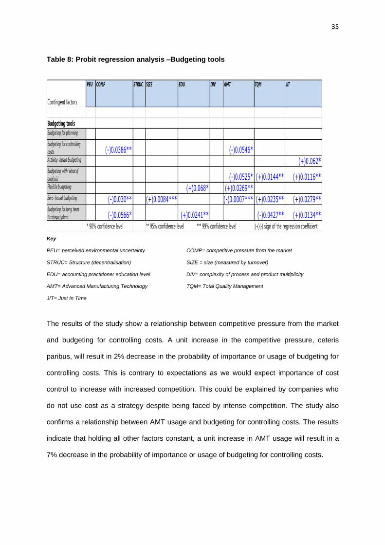
4.5.3 Factors affecting use of budgeting tools
Out of the seven budgeting tools investigated, budgeting for planning was the only tool that
could not be related to any of the nine contingent factors, see Table 8. This could be
attributable to the fact that regardless of circumstances organisations do budget for planning
purposes anyway. This can be supported by the 97.4% usage rate and stands out as the
highest among all 37 management accounting tools investigated.
35
Table 8: Probit regression analysis –Budgeting tools
Contingent factors
PEU COMP STRUC SIZE EDU DIV AMT TQM JIT
Budgeting for planning
Budgeting for controlling
costs (-)0.0386** (-)0.0546*Activity- based budgeting (+)0.062*Budgeting with 'what if
analysis' (-)0.0525* (+)0.0144** (+)0.0116**Flexible budgeting (+)0.068* (+)0.0269**Zero- based budgeting (-)0.030** (+)0.0084*** (-)0.0007*** (+)0.0235** (+)0.0279**Budgeting for long term
(strategic) plans (-)0.0566* (+)0.0241** (-)0.0427** (+)0.0134**
* 90% confidence level ** 95% confidence level *** 99% confidence level (+)(-) sign of the regression coefficient
Budgeting tools
Key
PEU= perceived environmental uncertainty COMP= competitive pressure from the market
STRUC= Structure (decentralisation) SIZE = size (measured by turnover)
EDU= accounting practitioner education level DIV= complexity of process and product multiplicity
AMT= Advanced Manufacturing Technology TQM= Total Quality Management
JIT= Just In Time
The results of the study show a relationship between competitive pressure from the market
and budgeting for controlling costs. A unit increase in the competitive pressure, ceteris
paribus, will result in 2% decrease in the probability of importance or usage of budgeting for
controlling costs. This is contrary to expectations as we would expect importance of cost
control to increase with increased competition. This could be explained by companies who
do not use cost as a strategy despite being faced by intense competition. The study also
confirms a relationship between AMT usage and budgeting for controlling costs. The results
indicate that holding all other factors constant, a unit increase in AMT usage will result in a
7% decrease in the probability of importance or usage of budgeting for controlling costs.
36
Activity based budgeting could only be linked to the use of JIT systems. A unit increase (all
other factors remaining constant) would result in a 3% increase in the probability of usage of
ABB. This confirms theory as in JIT environments activities consume resources which cause
costs (Kaplan, 1984; Kaplan & Atkinson, 1998).
Budgeting with what if analysis is used to solve complex management accounting problems
by bringing in different scenarios, (Kaplan & Atkinson, 1998). The study confirms that AMT
usage, TQM and JIT systems usage have an impact on the usage of budgeting with ‘what if’
analysis. Holding all other factors constant, a unit increase in the use of AMT decreases the
probability of importance or usage of ‘what if’ analysis by 7%. On the other hand a unit
increase in TQM or JIT (independently and holding other factors constant) usage will
increase the probability of importance of ‘what if’ analysis by 9%.
Flexible budgeting could only be linked to two contingent factors which are accounting
practitioner education and AMT usage. Holding other factors constant, a unit increase in
practitioner education or AMT will increase the probability of usage of flexible budgeting by
11% as shown in Appendix D (Equation 12).
Zero based budgeting could be linked to at least five of the nine contingent factors
investigated although it was the least used tool amongst the seven budgeting tools. A unit
increase, ceteris paribus, in competitive pressure from the market will reduce the probability
of importance of zero based budgeting, while a unit increase in size of organisation will
increase the probability of importance or usage of zero based budgeting. Abdel-Kader and
Luther (2008) found that a positive relationship exists between budgeting and the contingent
factors in their study on how firm specific characteristics affected management accounting
practices in the UK beverage industry. The bigger the organisation the more likely it is to
employ sophisticated budgeting tools. The results also confirm that holding other factors
constant, a unit increase in AMT usage will reduce the probability of the usage of zero based
37
budgeting by 6%. A unit increase in TQM and JIT (one at a time and holding other factors
constant) will increase the probability of usage of zero based budgeting by 4% and 3%
respectively. These results confirm the findings of Abdel-Kader and Luther (2008).
Budgeting for long term strategic plans could be linked to competitive pressure from the
market, accounting practitioner education level, TQM and JIT systems usage. All other
factors remaining the same, an increase in competitive pressure will result in a decrease in
the probability of importance of budgeting for long term strategic plans. The more intense the
level of competition we would expect organisations to craft long term strategies hence the
result is not as expected. However, the study suggests that firms that are not market leaders
in their industries end up focusing on short term strategies which in most cases are
reactionary. The more learned an accounting practitioner becomes the more they are likely
to employ modern management accounting tools (Graham & Harvey, 2001). This is
confirmed by the results where a unit increase in the education level, ceteris paribus, will
increase the probability of importance for long term strategic planning by 13,5%. A unit
increase in the use of TQM will result in a decrease in the probability of importance of
budgeting for long term strategic plans by 10%. Finally, a unit increase in JIT system usage
will increase the probability of usage of budgeting for long term strategic plans by 11.4%.
4.6 Performance evaluation tools Six performance evaluation tools were investigated. Benchmarking, economic value added
(EVA), non-financial measures related to employees, non-financial measures related to
operations and innovation, non-financial measures related to customers and ratio analysis
were the six tools investigated.
38
4.6.1 Performance evaluation tools usage
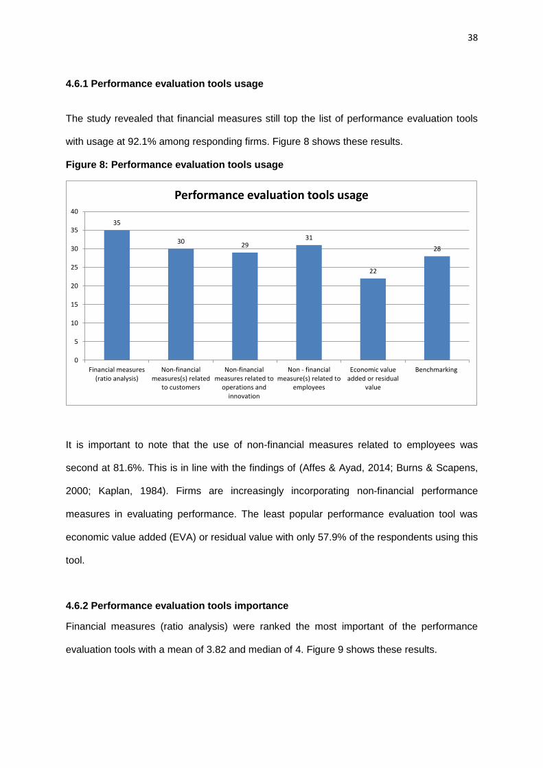
The study revealed that financial measures still top the list of performance evaluation tools
with usage at 92.1% among responding firms. Figure 8 shows these results.
Figure 8: Performance evaluation tools usage
35
3029
31
22
28
0
5
10
15
20
25
30
35
40
Financial measures(ratio analysis)
Non-financialmeasures(s) related
to customers
Non-financialmeasures related to
operations andinnovation
Non - financialmeasure(s) related to
employees
Economic valueadded or residual
value
Benchmarking
Performance evaluation tools usage
It is important to note that the use of non-financial measures related to employees was
second at 81.6%. This is in line with the findings of (Affes & Ayad, 2014; Burns & Scapens,
2000; Kaplan, 1984). Firms are increasingly incorporating non-financial performance
measures in evaluating performance. The least popular performance evaluation tool was
economic value added (EVA) or residual value with only 57.9% of the respondents using this
tool.
4.6.2 Performance evaluation tools importance
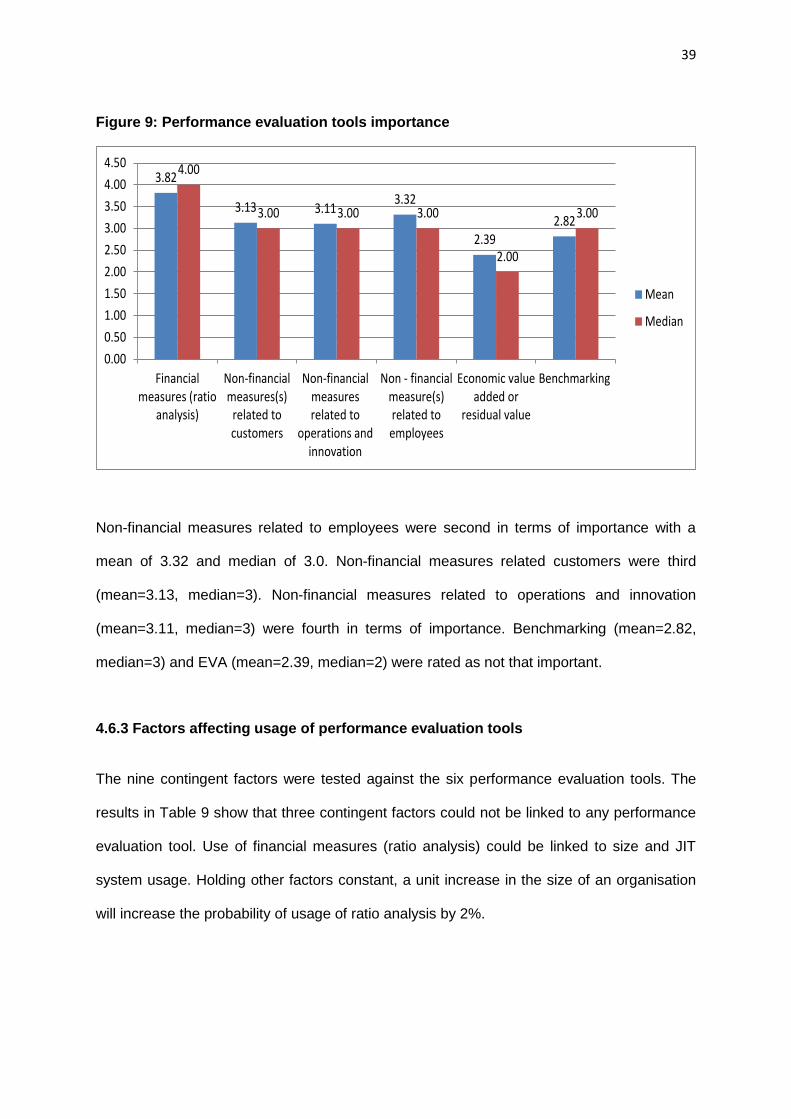
Financial measures (ratio analysis) were ranked the most important of the performance
evaluation tools with a mean of 3.82 and median of 4. Figure 9 shows these results.
39
Figure 9: Performance evaluation tools importance
3.82
3.13 3.113.32
2.392.82
4.00
3.00 3.00 3.00
2.00
3.00
0.00
0.50
1.00
1.50
2.00
2.50
3.00
3.50
4.00
4.50
Financialmeasures (ratio
analysis)
Non-financialmeasures(s)
related tocustomers
Non-financialmeasuresrelated to
operations andinnovation
Non - financialmeasure(s)related toemployees
Economic valueadded or
residual value
Benchmarking
Mean
Median
Non-financial measures related to employees were second in terms of importance with a
mean of 3.32 and median of 3.0. Non-financial measures related customers were third
(mean=3.13, median=3). Non-financial measures related to operations and innovation
(mean=3.11, median=3) were fourth in terms of importance. Benchmarking (mean=2.82,
median=3) and EVA (mean=2.39, median=2) were rated as not that important.
4.6.3 Factors affecting usage of performance evaluation tools
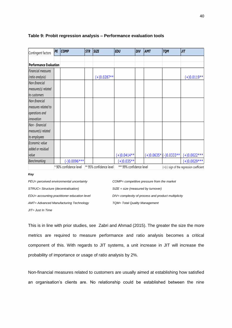
The nine contingent factors were tested against the six performance evaluation tools. The
results in Table 9 show that three contingent factors could not be linked to any performance
evaluation tool. Use of financial measures (ratio analysis) could be linked to size and JIT
system usage. Holding other factors constant, a unit increase in the size of an organisation
will increase the probability of usage of ratio analysis by 2%.
40
Table 9: Probit regression analysis – Performance evaluation tools
Contingent factors PE
U
COMP STR
UC
SIZE EDU DIV AMT TQM JIT
Financial measures
(ratio analysis) (+)0.0287** (+)0.0119**
Non-financial
measures(s) related
to customers
Non-financial
measures related to
operations and
innovation
Non - financial
measure(s) related
to employees
Economic value
added or residual
value (+)0.0414** (+)0.0635* (-)0.0333** (+)0.0022***
Benchmarking (-)0.0096*** (+)0.035** (+)0.0029***
* 90% confidence level ** 95% confidence level *** 99% confidence level (+)(-) sign of the regression coefficient
Performance Evaluation
Key
PEU= perceived environmental uncertainty COMP= competitive pressure from the market
STRUC= Structure (decentralisation) SIZE = size (measured by turnover)
EDU= accounting practitioner education level DIV= complexity of process and product multiplicity
AMT= Advanced Manufacturing Technology TQM= Total Quality Management
JIT= Just In Time
This is in line with prior studies, see Zabri and Ahmad (2015). The greater the size the more
metrics are required to measure performance and ratio analysis becomes a critical
component of this. With regards to JIT systems, a unit increase in JIT will increase the
probability of importance or usage of ratio analysis by 2%.
Non-financial measures related to customers are usually aimed at establishing how satisfied
an organisation’s clients are. No relationship could be established between the nine
41
contingent factors and use of non-financial measures related to customers. This could be
attributable to the size of the organisations in the sample.
Non-financial measures related to operations and innovations entail such measures as
process improvements and new product development. In this study no relationship could be
established between the nine contingent factors and use of non-financial measures related
to operations and innovation.
Non-financial measures related to employees look at aspects such as employee
engagement levels. The results of the study show that no relationship exists between the
nine contingent factors and use of non-financial measures related to employees suggesting
that there could be other factors responsible for this based on the 81.6% usage rate in the
sample.
Use of EVA or residual value could be linked to four contingent factors indicating that a
relationship does exist between the contingent factors and use of EVA. According to the
study accounting practitioner education level has an impact on the use of EVA. Holding other
factors constant, a unit increase in accounting practitioner education level will increase the
probability of usage of EVA by 15%, while a unit increase in AMT would increase the
probability of EVA usage by 10%. A unit increase in TQM will decrease the probability of
EVA usage by 12% while a unit increase in JIT usage increases the probability of usage by
16%. The application of these tools requires high levels of education as many adjustments
need to be applied to financials to determine EVA. It is expected that these techniques would
be applied in technologically advanced industries by qualified personnel.
The results of the study indicate that an increase in competitive pressure would reduce the
importance of benchmarking. This is contrary to expectations as companies are expected to
use benchmarking the more competitive the environment is. An increase accounting
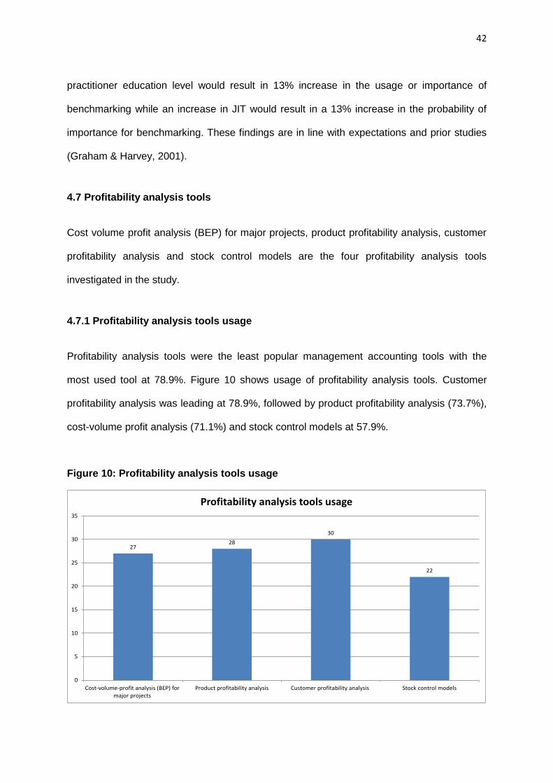
42
practitioner education level would result in 13% increase in the usage or importance of
benchmarking while an increase in JIT would result in a 13% increase in the probability of
importance for benchmarking. These findings are in line with expectations and prior studies
(Graham & Harvey, 2001).
4.7 Profitability analysis tools
Cost volume profit analysis (BEP) for major projects, product profitability analysis, customer
profitability analysis and stock control models are the four profitability analysis tools
investigated in the study.
4.7.1 Profitability analysis tools usage
Profitability analysis tools were the least popular management accounting tools with the
most used tool at 78.9%. Figure 10 shows usage of profitability analysis tools. Customer
profitability analysis was leading at 78.9%, followed by product profitability analysis (73.7%),
cost-volume profit analysis (71.1%) and stock control models at 57.9%.
Figure 10: Profitability analysis tools usage
2728
30
22
0
5
10
15
20
25
30
35
Cost-volume-profit analysis (BEP) formajor projects
Product profitability analysis Customer profitability analysis Stock control models
Profitability analysis tools usage
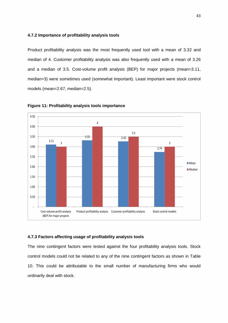
43
4.7.2 Importance of profitability analysis tools
Product profitability analysis was the most frequently used tool with a mean of 3.32 and
median of 4. Customer profitability analysis was also frequently used with a mean of 3.26
and a median of 3.5. Cost-volume profit analysis (BEP) for major projects (mean=3.11,
median=3) were sometimes used (somewhat important). Least important were stock control
models (mean=2.67, median=2.5).
Figure 11: Profitability analysis tools importance
3.11 3.32 3.26
2.74
3
4
3.5
3
-
0.50
1.00
1.50
2.00
2.50
3.00
3.50
4.00
4.50
Cost-volume-profit analysis(BEP) for major projects
Product profitability analysis Customer profitability analysis Stock control models
Mean
Median
4.7.3 Factors affecting usage of profitability analysis tools
The nine contingent factors were tested against the four profitability analysis tools. Stock
control models could not be related to any of the nine contingent factors as shown in Table
10. This could be attributable to the small number of manufacturing firms who would
ordinarily deal with stock.
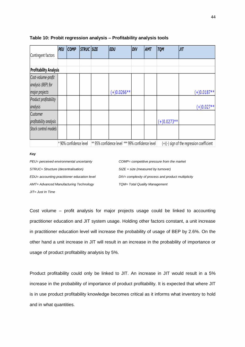
44
Table 10: Probit regression analysis – Profitability analysis tools
Contingent factors
PEU COMP STRUC SIZE EDU DIV AMT TQM JIT
Cost-volume-profit
analysis (BEP) for
major projects (+)0.0266** (+)0.0187**
Product profitability
analysis (+)0.027**
Customer
profitability analysis (+)0.0273**
Stock control models
* 90% confidence level ** 95% confidence level *** 99% confidence level (+)(-) sign of the regression coefficient
Profitability Analysis
Key
PEU= perceived environmental uncertainty COMP= competitive pressure from the market
STRUC= Structure (decentralisation) SIZE = size (measured by turnover)
EDU= accounting practitioner education level DIV= complexity of process and product multiplicity
AMT= Advanced Manufacturing Technology TQM= Total Quality Management
JIT= Just In Time
Cost volume – profit analysis for major projects usage could be linked to accounting
practitioner education and JIT system usage. Holding other factors constant, a unit increase
in practitioner education level will increase the probability of usage of BEP by 2.6%. On the
other hand a unit increase in JIT will result in an increase in the probability of importance or
usage of product profitability analysis by 5%.
Product profitability could only be linked to JIT. An increase in JIT would result in a 5%
increase in the probability of importance of product profitability. It is expected that where JIT
is in use product profitability knowledge becomes critical as it informs what inventory to hold
and in what quantities.
45
Holding other factors constant an increase in TQM would increase the probability of
importance of customer profitability analysis by 9%. Where TQM is practiced it becomes
imperative to focus on overall profitability of a customer as clients may require different
standards or additional services. These results are in line with expectations.
4.8 Investment decision making tools Five investment decision making tool were investigated as shown in Figure 12.
4.8.1 Investment decision making tools usage At least 81.6% of the respondents used at least one of the selected investment decision
making tools. The most popular was the documentation and reporting of non-financial
aspects in evaluating major capital investments. This indicates a shift from the traditional
approach where firms would make investment decisions based only on financial measures,
(Graham & Harvey, 2001). The least used investment tool was the use of probability analysis
and computer simulation in evaluating major capital projects. This could be attributed to the
size of the firms in the sample. The average annual turnover of the responding firms was
between R100 million to R500 million. While use of discounted cash flows (DCF) in
evaluating major capital investment was at 73.7%.
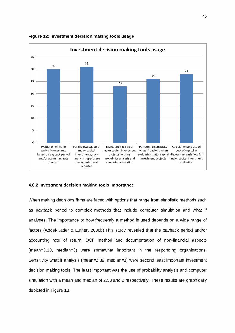
46
Figure 12: Investment decision making tools usage
3031
23
26
28
0
5
10
15
20
25
30
35
Evaluation of majorcapital investments
based on payback periodand/or accounting rate
of return
For the evaluation ofmajor capital
investments, non-financial aspects are
documented andreported
Evaluating the risk ofmajor capital investment
projects by usingprobability analysis and
computer simulation
Performing sensitivity'what if' analysis when
evaluating major capitalinvestment projects
Calculation and use ofcost of capital in
discounting cash flow formajor capital investment
evaluation
Investment decision making tools usage
4.8.2 Investment decision making tools importance
When making decisions firms are faced with options that range from simplistic methods such
as payback period to complex methods that include computer simulation and what if
analyses. The importance or how frequently a method is used depends on a wide range of
factors (Abdel-Kader & Luther, 2006b).This study revealed that the payback period and/or
accounting rate of return, DCF method and documentation of non-financial aspects
(mean=3.13, median=3) were somewhat important in the responding organisations.
Sensitivity what if analysis (mean=2.89, median=3) were second least important investment
decision making tools. The least important was the use of probability analysis and computer
simulation with a mean and median of 2.58 and 2 respectively. These results are graphically
depicted in Figure 13.
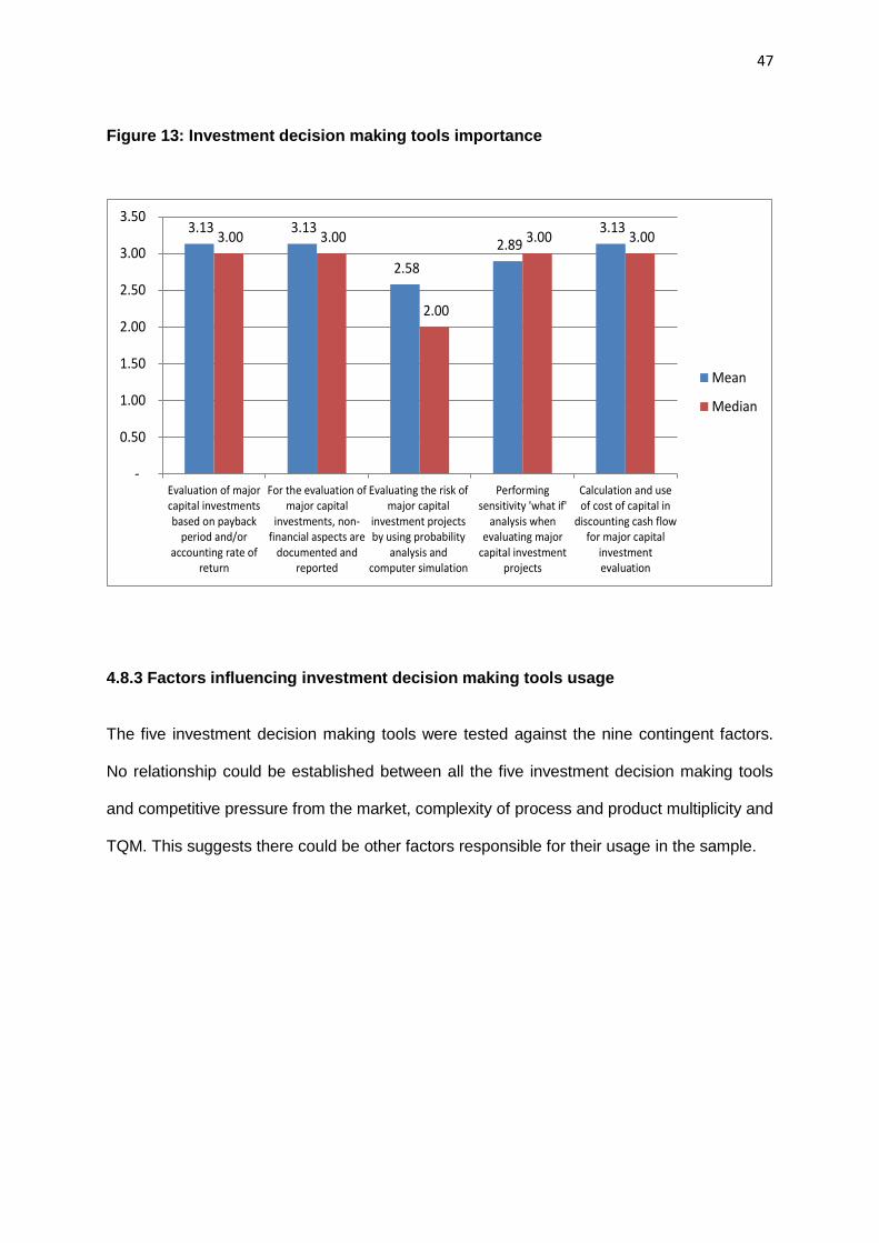
47
Figure 13: Investment decision making tools importance
3.13 3.13
2.58
2.89 3.13
3.00 3.00
2.00
3.00 3.00
-
0.50
1.00
1.50
2.00
2.50
3.00
3.50
Evaluation of majorcapital investmentsbased on payback
period and/oraccounting rate of
return
For the evaluation ofmajor capital
investments, non-financial aspects are
documented andreported
Evaluating the risk ofmajor capital
investment projectsby using probability
analysis andcomputer simulation
Performingsensitivity 'what if'
analysis whenevaluating major
capital investmentprojects
Calculation and useof cost of capital in
discounting cash flowfor major capital
investmentevaluation
Mean
Median
4.8.3 Factors influencing investment decision making tools usage
The five investment decision making tools were tested against the nine contingent factors.
No relationship could be established between all the five investment decision making tools
and competitive pressure from the market, complexity of process and product multiplicity and
TQM. This suggests there could be other factors responsible for their usage in the sample.
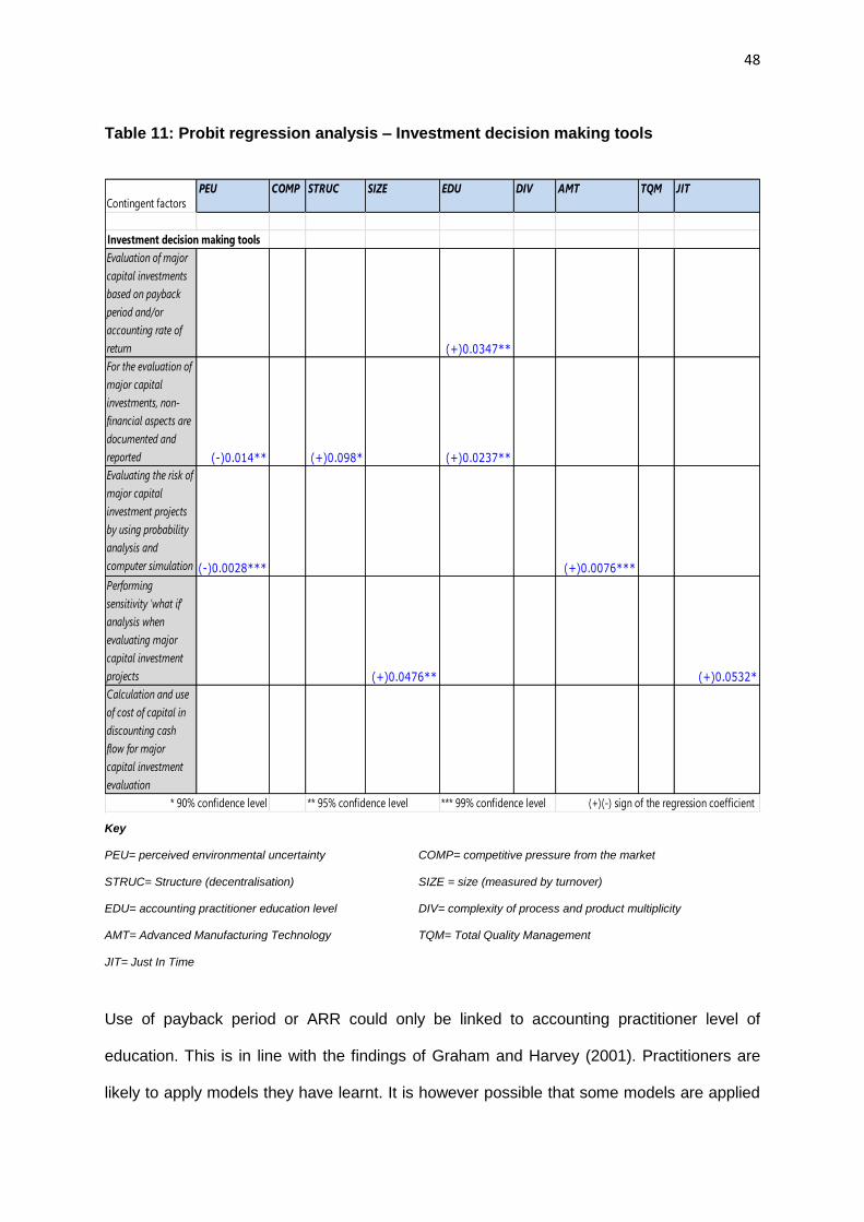
48
Table 11: Probit regression analysis – Investment decision making tools
Contingent factors
PEU COMP STRUC SIZE EDU DIV AMT TQM JIT
Evaluation of major
capital investments
based on payback
period and/or
accounting rate of
return (+)0.0347**
For the evaluation of
major capital
investments, non-
financial aspects are
documented and
reported (-)0.014** (+)0.098* (+)0.0237**
Evaluating the risk of
major capital
investment projects
by using probability
analysis and
computer simulation (-)0.0028*** (+)0.0076***
Performing
sensitivity 'what if'
analysis when
evaluating major
capital investment
projects (+)0.0476** (+)0.0532*
Calculation and use
of cost of capital in
discounting cash
flow for major
capital investment
evaluation
* 90% confidence level ** 95% confidence level *** 99% confidence level (+)(-) sign of the regression coefficient
Investment decision making tools
Key
PEU= perceived environmental uncertainty COMP= competitive pressure from the market
STRUC= Structure (decentralisation) SIZE = size (measured by turnover)
EDU= accounting practitioner education level DIV= complexity of process and product multiplicity
AMT= Advanced Manufacturing Technology TQM= Total Quality Management
JIT= Just In Time
Use of payback period or ARR could only be linked to accounting practitioner level of
education. This is in line with the findings of Graham and Harvey (2001). Practitioners are
likely to apply models they have learnt. It is however possible that some models are applied
49
dictated by company policy. We may probably want to then trace the origins of such policy
and it may not be surprising that we come back to accounting practitioner education level.
Holding other factors constant, a unit increase in accounting practitioner education level
increases the probability of usage of ARR by 0.3%.
Perceived environmental uncertainty was found to have an impact on documentation of non-
financial aspects in the evaluation of major capital projects. The results show that holding
other factors constant, a unit increase in PEU decreases the probability of the usage of
documentation of non-financial information related to major capital projects by 1.4%. This is
not as expected and maybe due to lack of awareness of the importance of non-financial
aspects. Alternatively, decision making could still be driven by financial analysis with
accountants not comfortable investigating non-financial aspects which are difficult to
quantify. A unit increase in structure (decentralisation) increases the probability of usage by
8%. A unit increase in practitioner education level increases the probability of usage by 13%.
Use of probability analysis and computer simulation in the evaluation of major capital
investment projects could be related to two factors only. Holding other factors constant, a
unit increase in PEU decreases the probability of usage of computer simulation or probability
analysis by 6%. This is in contrast to what theory suggests. As the environment becomes
uncertain the more we expect more complex models to be used applying some simulation
and probability analysis. This result could be attributable to the size of organisations in the
sample. A unit increase in AMT usage increases the probability of usage of probability
analysis or computer simulation by 4%.
Use of sensitivity ‘what if’ analysis could be linked to organisational size and JIT usage.
Holding other factors constant, a unit increase in size increases the probability of usage of
‘what if’ analysis by 2% while a unit increase in JIT usage increases the probability by 2%.
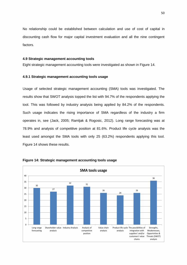
50
No relationship could be established between calculation and use of cost of capital in
discounting cash flow for major capital investment evaluation and all the nine contingent
factors.
4.9 Strategic management accounting tools
Eight strategic management accounting tools were investigated as shown in Figure 14.
4.9.1 Strategic management accounting tools usage
Usage of selected strategic management accounting (SMA) tools was investigated. The
results show that SWOT analysis topped the list with 94.7% of the respondents applying the
tool. This was followed by industry analysis being applied by 84.2% of the respondents.
Such usage indicates the rising importance of SMA regardless of the industry a firm
operates in, see (Jack, 2005; Ramljak & Rogosic, 2012). Long range forecasting was at
78.9% and analysis of competitive position at 81.6%. Product life cycle analysis was the
least used amongst the SMA tools with only 25 (63.2%) respondents applying this tool.
Figure 14 shows these results.
Figure 14: Strategic management accounting tools usage
30
27
3231
2624
26
36
0
5
10
15
20
25
30
35
40
Long rangeforecasting
Shareholder valueanalysis
Industry Analysis Analysis ofcompetitive
position
Value chainanalysis
Product life cycleanalysis
The possibilities ofintegration withsuppliers' and/orcustomers' value
chains
Strengths,Weakenesses,Opportnities &Threats (SWOT)
analysis
SMA tools usage
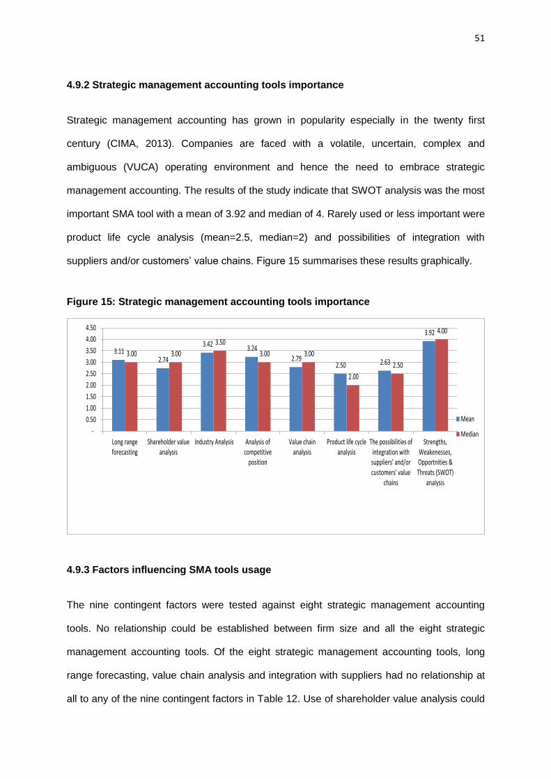
51
4.9.2 Strategic management accounting tools importance
Strategic management accounting has grown in popularity especially in the twenty first
century (CIMA, 2013). Companies are faced with a volatile, uncertain, complex and
ambiguous (VUCA) operating environment and hence the need to embrace strategic
management accounting. The results of the study indicate that SWOT analysis was the most
important SMA tool with a mean of 3.92 and median of 4. Rarely used or less important were
product life cycle analysis (mean=2.5, median=2) and possibilities of integration with
suppliers and/or customers’ value chains. Figure 15 summarises these results graphically.
Figure 15: Strategic management accounting tools importance
3.11 2.74
3.42 3.24
2.79 2.50 2.63
3.92
3.00 3.00
3.50
3.00 3.00
2.00
2.50
4.00
-
0.50
1.00
1.50
2.00
2.50
3.00
3.50
4.00
4.50
Long rangeforecasting
Shareholder valueanalysis
Industry Analysis Analysis ofcompetitive
position
Value chainanalysis
Product life cycleanalysis
The possibilities ofintegration withsuppliers' and/orcustomers' value
chains
Strengths,Weakenesses,Opportnities &Threats (SWOT)
analysis
Mean
Median
4.9.3 Factors influencing SMA tools usage
The nine contingent factors were tested against eight strategic management accounting
tools. No relationship could be established between firm size and all the eight strategic
management accounting tools. Of the eight strategic management accounting tools, long
range forecasting, value chain analysis and integration with suppliers had no relationship at
all to any of the nine contingent factors in Table 12. Use of shareholder value analysis could
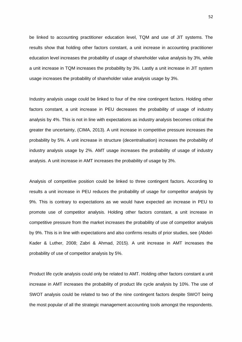
52
be linked to accounting practitioner education level, TQM and use of JIT systems. The
results show that holding other factors constant, a unit increase in accounting practitioner
education level increases the probability of usage of shareholder value analysis by 3%, while
a unit increase in TQM increases the probability by 3%. Lastly a unit increase in JIT system
usage increases the probability of shareholder value analysis usage by 3%.
Industry analysis usage could be linked to four of the nine contingent factors. Holding other
factors constant, a unit increase in PEU decreases the probability of usage of industry
analysis by 4%. This is not in line with expectations as industry analysis becomes critical the
greater the uncertainty, (CIMA, 2013). A unit increase in competitive pressure increases the
probability by 5%. A unit increase in structure (decentralisation) increases the probability of
industry analysis usage by 2%. AMT usage increases the probability of usage of industry
analysis. A unit increase in AMT increases the probability of usage by 3%.
Analysis of competitive position could be linked to three contingent factors. According to
results a unit increase in PEU reduces the probability of usage for competitor analysis by
9%. This is contrary to expectations as we would have expected an increase in PEU to
promote use of competitor analysis. Holding other factors constant, a unit increase in
competitive pressure from the market increases the probability of use of competitor analysis
by 9%. This is in line with expectations and also confirms results of prior studies, see (Abdel-
Kader & Luther, 2008; Zabri & Ahmad, 2015). A unit increase in AMT increases the
probability of use of competitor analysis by 5%.
Product life cycle analysis could only be related to AMT. Holding other factors constant a unit
increase in AMT increases the probability of product life cycle analysis by 10%. The use of
SWOT analysis could be related to two of the nine contingent factors despite SWOT being
the most popular of all the strategic management accounting tools amongst the respondents.
53
Holding other factors constant, a unit increase in complexity of process and product
multiplicity increases the probability of SWOT usage by 0.9% while a unit increase in AMT
decreases the probability by 0.6%.
Table 12: Probit regression analysis – SMA tools
Contingent factorsPEU COMP STRUC SIZE EDU DIV AMT TQM JIT
Long range
forecasting
Shareholder value
analysis (+)0.053* (+)0.0581* (+)0.0419**
Industry Analysis (-)0.0051*** (+)0.0023*** (+)0.0367** (+)0.0119**
Analysis of
competitive position
(-)0.0171** (+)0.371** (+)0.0946*
Value chain analysis
Product life cycle
analysis(+)0.05**
The possibilities of
integration with
suppliers' and/or
customers' value
chains
Strengths,
Weakenesses,
Opportnities &
Threats (SWOT)
analysis (+)0.0067*** (-)0.0483**
* 90% confidence level ** 95% confidence level *** 99% confidence level (+)(-) sign of the regression coefficient
Strategic Management Accounting
Key
PEU= perceived environmental uncertainty COMP= competitive pressure from the market
STRUC= Structure (decentralisation) SIZE = size (measured by turnover)
EDU= accounting practitioner education level DIV= complexity of process and product multiplicity
AMT= Advanced Manufacturing Technology TQM= Total Quality Management
JIT= Just In Time
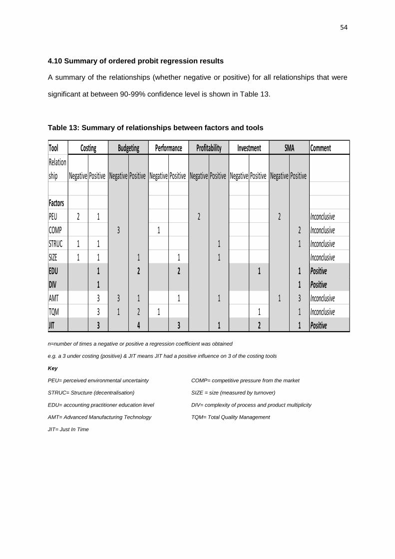
54
4.10 Summary of ordered probit regression results
A summary of the relationships (whether negative or positive) for all relationships that were
significant at between 90-99% confidence level is shown in Table 13.
Table 13: Summary of relationships between factors and tools
Tool Comment
Relation
ship Negative Positive Negative Positive Negative Positive Negative Positive Negative Positive Negative Positive
Factors
PEU 2 1 2 2 Inconclusive
COMP 3 1 2 Inconclusive
STRUC 1 1 1 1 Inconclusive
SIZE 1 1 1 1 1 Inconclusive
EDU 1 2 2 1 1 Positive
DIV 1 1 Positive
AMT 3 3 1 1 1 1 3 Inconclusive
TQM 3 1 2 1 1 1 Inconclusive
JIT 3 4 3 1 2 1 Positive
Costing Budgeting Performance Profitability Investment SMA
n=number of times a negative or positive a regression coefficient was obtained
e.g. a 3 under costing (positive) & JIT means JIT had a positive influence on 3 of the costing tools
Key
PEU= perceived environmental uncertainty COMP= competitive pressure from the market
STRUC= Structure (decentralisation) SIZE = size (measured by turnover)
EDU= accounting practitioner education level DIV= complexity of process and product multiplicity
AMT= Advanced Manufacturing Technology TQM= Total Quality Management
JIT= Just In Time
55
4.11 Other factors affecting management accounting tools usage The study inquired about other factors that affected management accounting practices in the
responding organisations through open ended questions in the questionnaire. Most of the
factors highlighted were just semantically different from the nine contingent factors that
formed part of the study. The following are however worth noting.
4.11.1 Requirements by providers of funds
This response came mainly from the non-governmental organisations where providers of
funds required their beneficiaries to provide specific reports relating to their activities and
funding. In this category respondents indicated that the choice of which management
accounting tools to use was predominantly determined by their sponsors.
4.11.2 Change in legislation affecting industry
Legislation passed by national governments may force companies to use certain
management accounting tools as they seek to comply with certain directives. Of note in
South Africa is the need to comply with Black Economic Empowerment (BEE) where there
are certain prescribed ratios e.g. what percentage of an organisation’s profit must be
channelled towards enterprise development? In this instance organisations are required to
adopt certain profitability measurement tools.
4.11.3 Industry practice This is more of an institutional factor were there are specific taken for granted rules within an
industry. Where industry is heavily unionised, and unions use certain parameters to bargain
for wage increases, players in the industry are likely to adopt certain management
accounting tools. This is line with the work of Scapens (2006).

56
4.11.4 Head office practice
Some South African companies who were subsidiaries of international companies confirmed
that they had no say as to which management accounting tools should be used but instead
the head offices dictated what accounting tools must be used depending on their information
requirements.
57
Chapter V Conclusion and recommendations
The study has investigated the application of management accounting tools in South Africa
through an online survey questionnaire using a sample of 942 respondents and achieved a
response rate of 7% before data cleaning. The results confirm usage of all the six (37 tools
in total) management accounting tool categories by firms in South Africa. While the study
confirmed use of all the 37 management accounting tools, the importance attached to each
tool as measured by the means and medians varied widely per category. The most
frequently (regarded as more important) used were budgets followed by SMA tools,
performance evaluation tools, costing tools, profitability analysis tools and finally investment
decision making tools.
An analysis of the contingent factors affecting usage of the management accounting tools
revealed that twenty seven of the thirty-seven management accounting tools could be
related to at least one of the selected nine contingent factors. The study could however not
conclusively establish a positive relationship between the contingent factors and the
management accounting tools. Ignoring cases where no relationships could be established
between contingent factors and the tools, only three of the nine contingent factors had a
positive influence on management accounting tools used. These factors include accounting
practitioner education level, diversity of process and product multiplicity and JIT. Results for
the other six contingent factors were inconclusive as contingent factors had both negative
and positive influences on management accounting tools usage e.g. PEU (Table 13) had
both negative and positive influence on costing tools, depending on the tool analysed. The
researcher would recommend further studies on how contingent factors influence
management accounting practice as this study was inconclusive on these other factors.
As mentioned earlier one of the limitations of this study was that it was not industry specific
and did not look at specific organisational size. The researcher recommends that a similar
58
study be carried out focusing on specific company size as measured using number of
employees, annual turnover or total assets.
The results show that perceived environmental uncertainty seemed not to influence usage of
management accounting tools. The researcher recommends that case studies be used to
gather an in-depth understanding of how South African companies operate, and how they
deal with uncertainty. This will shed more light as to why some of the results obtained were
not as expected.
Finally, as this study was not industry sector specific, the researcher recommends a sector
specific study be carried out in South Africa e.g. mining sector or insurance sector. This will
assist in gaining a better understanding on how contingent factors play a role in those
sectors, and the results obtained may be more consistent than the ones found in the present
study.
59
References
Abdel-Kader, M., & Luther, R. (2006a). IFAC's Conception of the Evolution of Management Accounting. Advances in Management Accounting, 15, 229-247.
Abdel-Kader, M., & Luther, R. (2006b). Management accounting practices in the UK food and drinks industry. London: Chartered Institute of Management Accountants (CIMA).
Abdel-Kader, M., & Luther, R. (2008). The Impact of Firm Characteristics on Management Accounting Practices: A UK Based Empirical Analysis. The British Accounting Review, 40(1), 2-27. doi: DOI: 10.1016/j.bar.2007.11.003
Affes, H., & Ayad, F. (2014). Contextual factors impact on the use of new management accounting practices: An Empirical analysis in the Tunisian context. Journal of Research in International Business and Management, 4(3), 45-55. doi: http:/dx.doi.org/10.14303/jribm.2014.010
Ahmad, N. S. M., & Leftesi, A. (2014). An Exploratory Study of the Level of Sophistication of Management Accounting Practices in Libyan Manufacturing Companies. International Journal of Business and Management, II(2), 1-8.
AICPA. (2017). Global management accounting principles. London: Association of International Certified Professional Accountants (AICPA)
Al-Mawali, H. (2015). Contingent factors of Strategic Management Accounting. Research Journal of Finance and Accounting 6(11), 130-138.
Albright, T., & Lam, M. (2006). Managerial accounting and continuous improvement initiatives: A retrospective and framework. Journal of Managerial Issues, 18(2), 157-175.
Alleyne, P., & Weeks-Marshal, D. (2011). An Exploratory Study of Management Accounting Practices in Manufacturing Companies in Barbados. International Journal of Business and Social Science, 2(9), 49-58.
Askrany, D. (2005). The evolution of management accounting innovations and the level of satisfaction with traditional accounting techniques. Paper presented at the AFAANZ Conference, Melbourne, Australia.
Baldvinsdottir, G., Mitchell, F., & Norreklit, H. (2010). Issues in the relationship between theory and practice in management accounting. Management Accounting Research, 21(2), 79-82.
Burns, J., Ezzamel, M., & Scapens, R. W. (2003). The Challenge of Management Accounting Change: Behavioural and Cultural Aspects of Change Management CIMA Publishing/Elsevier, London/Oxford.
Burns, J., & Scapens, R. W. (2000). Conceptualising Management Accounting Change: An Institutional Framework. Management Accounting Research, 11(1), 3-25.
Burns, J., & Vaivio, J. (2001). Management accounting change. Management Accounting Research, 12, 389-402. doi: 10.1006/mare.2001.0178
60
Chenhall, R. H. (2003). Management control systems design within its organisational context: findings from contingency-based research and directions for the future. Accounting Organisations and Society, 28, 127-168.
CIMA. (2009). Management accounting tools for today and tomorrow. London: Chartered Institute Management Accountants.
CIMA. (2013). Essential tools for management accountants.The tools and techniques to support sustainable business success. London: Chartered Institute of Management Accountants (CIMA)
DiMaggio, P. J., & Powell, W. (1983). The iron cage revisited: Institutional isomorphism and collective rationality in organisational fields. American Sociological Review, 48(2), 147-160.
Dropulic, I. (2013). The effect of contingency factors on management control Systems: A study of manufacturing companies in Croatia. Ekonomska istrazivanja-Economic Research (Special Issue), 369-382
Drury, C., & Al-Omiria, M. (2007). A survey of factors influencing the choice of product costing systems in UK organisations. Management Accounting Research, 18(4), 399-424.
Drury, C., & Tayles, M. (1994). Product costing in UK manufacturing organisations. The European Accounting Review, 3(3), 443-469.
Dugdale, D., Jones, C., & Green, S. (2005). Contemporary management accounting practices in UK manufacturing (Vol. 1). London: Elsevier.
Fakoya, M. B. (2014). On Managerial Accounting Practices in South African Public Departments. Journal of Economics, 5(2), 133-139.
Garg, A., Ghosh, D., Hudick, J., & Nowacki, C. (2003). Roles and Practices in Management Accounting Today London: Institute of Management Accountants - Ernst & Young.
Gordon, L. A., & Miller, D. (1976). A contingency framework for the design of accounting information systems. Accounting, Organisations and Society, 1(1), 59-69.
Graham, J. R., & Harvey, C. R. (2001). How do CFOs make capital budgeting and capital structure decisions? The Journal of Applied Corporate Finance 15(1), 265-301.
IFAC. (1998). International Management Accounting Practice Statement: Management Accounting Concepts. (pp. 82-100). New York: Financial and Management Accounting Committee.
Ittner, C. D., & Larcker, D. F. (1998). Innovations in performance measurement:Trends and research implications. Journal of Management Accounting Research, 10, 205-238.
Jack, L. (2005). The adoption of strategic management accounting tools in agriculture post subsidy reform: a comparative study of practices in the UK, the US, Australia and New Zealand Research executive summary
(Vol. 5, pp. 1-7). London: Chartered Institute on Management Accountants.
61
Jinga, G., & Dumitru, M. (2015). The Management Accounting Tools and the Integrated Reporting. SEA - Practical Application of Science, III(1(7)), 45-50.
Johnson, H. T., & Kaplan, R. S. (1987). Relevance lost: The rise and fall of management accounting. Boston, Massachusetts: Harvard Business School Press.
Kaplan, R. S. (1984). The Evolution of Management Accounting. The Accounting Review, LIX, No.3, 390-418.
Kaplan, R. S., & Atkinson, A. A. (1998). Advanced Management Accounting (3rd ed.). New Jersey: Prentice Hall, Inc.
Kaplan, R. S., & Cooper, R. (1998). Cost & Effect: Using Integrated Cost Systems to Drive Profitability and Performance: Harvard Business School Press.
Langfield-Smith, K., & Chenhall, R. H. (1998). Adoption and benefits of management accounting practices: an Australian study. Management Accounting Research, 9, 1-19.
Mat, T. Z. T. (2013). Theoretical framework on management accounting and organisational change. Asia Pacific Management Accounting Journal, 9(2), 85-105.
McNally, G. M., & Lee, H. E. (1980). Management Accounting Practices and Company Characteristics. ABACUS, 16(2), 142-150.
Montvale, N. J. (1994). What Corporate America wants in entry level accountants. New York: Institute of Management Accountants.
Ramljak, B., & Rogosic, A. (2012). Strategic Management Accounting Practices in Croatia. The Journal of International Management Studies, 7(2), 93-100.
Robalo, R. (2014). Explanations for the gap between management accounting rules and routines: An institutional approach. Spanish Accounting Review, 17(2), 88-97.
Roslender, R. (1996). Relevance lost and found:Critical perspectives on the promise of management accounting. Critical Perspectives on Accounting, 7, 533-561.
Scapens, R. W. (1994). Never Mind the Gap: Towards an Institutional Perspective of Management Accounting Practices. Management Accounting Research, 5(3/4), 301-321. doi: 10.1006/mare.1994.1019
Scapens, R. W. (2006). Understanding management accounting practices: A personal journey. The British Accounting Review, 38, 1-30.
Sharaf - Addin, H., Omar, N., & Sulaiman, S. (2014). Target Costing Evolution: A Review of the Literature from IFAC's (1998) Model. Asian Social Science, 10(9), 82-99.
Sharkar, M. Z. H., Sobhan, M. A., & Sultana, S. (2006). Management Accounting Development and Practices in Bangladesh. BRAC University Journal, III(2), 113-124.
Uyar, A. (2010). Cost and management accounting practices: A survey of manufacturing companies. Eurasian Journal of Business and Economics, 3(6), 113-125.

62
Wanderley, C. D., Miranda, L. C., De Meira, J. M., & Cullen, J. (2011). Management Accounting Change: A model based on three different theoretical frameworks. BASE-REVISTA ADMINISTRACAO E CONTABILIDADE DA UNISINOS, 8(2), 111-121.
Waweru, N. M., Hoque, Z., & Uliana, E. (2005). A Survey of Management Accounting practices in South Africa: Case Study of Retail Services. Journal of Accounting, Auditing and Performance Evaluation, 2(3), 22-29.
Wijewardena, H., & De Zoysa, A. (1999). Comparative Analysis of Management Accounting Practices in Australia and Japan: An Empirical Investigation. The International Journal of Accounting, 34(1), 49-70.
Zabri, M. S., & Ahmad, K. (2015). Factors explaining the use of management accounting practices in Malaysian medium-sized firms. Journal of Small Business and Enterprise Development, 22(4), 762-781. doi: 10.1108/JSBED-04-2012-0057
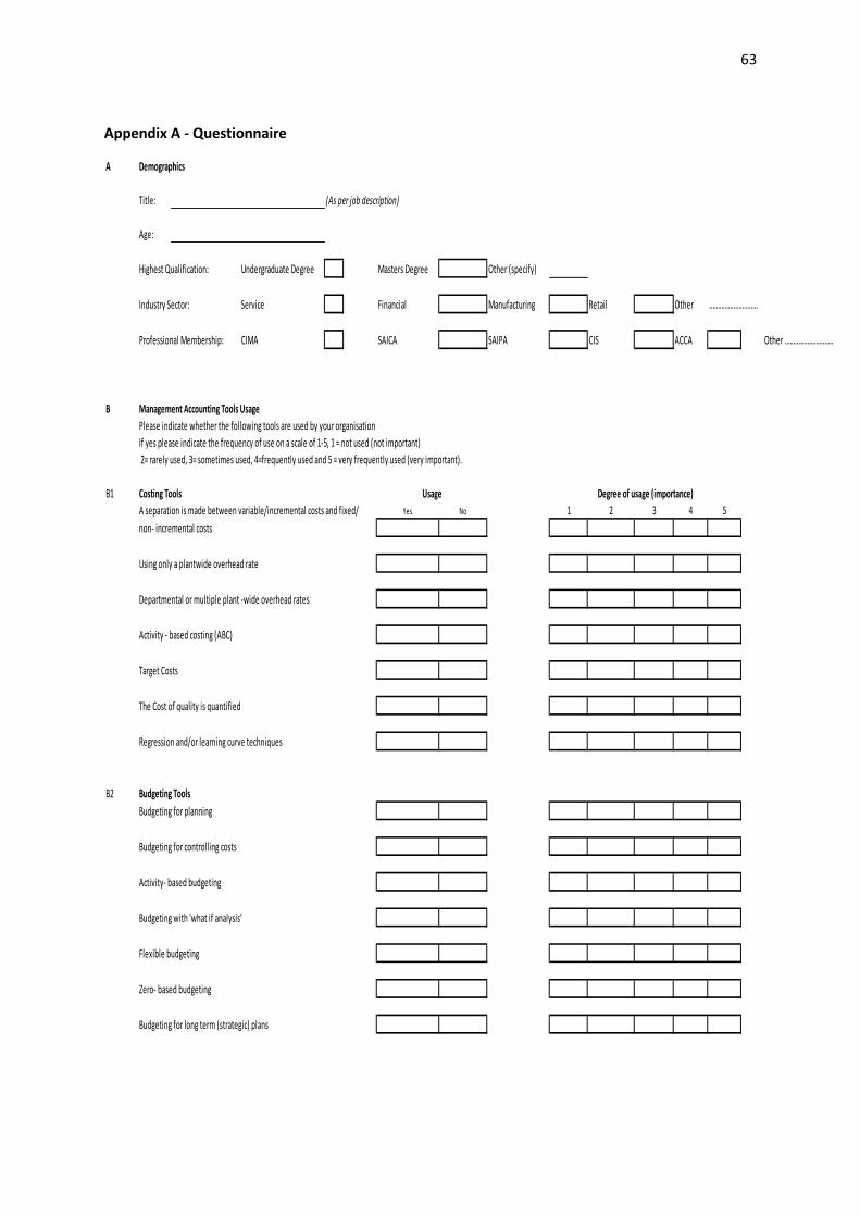
63
Appendix A - Questionnaire
A Demographics
Title: (As per job description)
Age:
Highest Qualification: Undergraduate Degree Masters Degree Other (specify)
Industry Sector: Service Financial Manufacturing Retail Other ……………………….
Professional Membership: CIMA SAICA SAIPA CIS ACCA Other (specify):……………………….
B Management Accounting Tools Usage
Please indicate whether the following tools are used by your organisation
If yes please indicate the frequency of use on a scale of 1-5, 1 = not used (not important)
2= rarely used, 3= sometimes used, 4=frequently used and 5 = very frequently used (very important).
B1 Costing Tools
A separation is made between variable/incremental costs and fixed/ Yes No 1 2 3 4 5
non- incremental costs
Using only a plantwide overhead rate
Departmental or multiple plant -wide overhead rates
Activity - based costing (ABC)
Target Costs
The Cost of quality is quantified
Regression and/or learning curve techniques
B2 Budgeting Tools
Budgeting for planning
Budgeting for controlling costs
Activity- based budgeting
Budgeting with 'what if analysis'
Flexible budgeting
Zero- based budgeting
Budgeting for long term (strategic) plans
Degree of usage (importance)Usage
64
B3 Performance Evaluation Tools
Financial measures (ratio analysis)
Non-financial measures(s) related to customers
Non-financial measures related to operations and innovation
Non - financial measure(s) related to employees
Economic value added or residual value
Benchmarking
B4 Profitability Analysis Tools
Cost-volume-profit analysis (BEP) for major projects
Product profitability analysis
Customer profitability analysis
Stock control models
B5 Investment decision making tools
Evaluation of major capital investments based on
payback period and/or accounting rate of return
For the evaluation of major capital investments, non-financial aspects are
doucumeted and reported
Evaluating the risk of major capital investment projects
by using probability analysis and computer simulation
Perfoming sensitivity 'what if' analsysis when evaluationg
major capital investment projects
Calculation and use of cost of capital in discounting cash flow
for major capital investment evaluation
65
B6 Strategic Management Accounting Tools
Long range forecasting
Shareholder value analysis
Industry Analysis
Analysis of competitive position
Value chain analysis
Product life cycle analysis
The possibilities of integration with suppliers' and/
or customers' value chains
Strengths, Weakenesses, Opportnities & Threats (SWOT) analysis
C Using the given scales, kindly rate the following contingent factors for your organisation
1 2 3 4 5
Perceived Environmental Uncertainty (PEU)
On a scale of 1-5 indicate how predictible your external environment is
including suppliers, competitors, customers and government
1=highly predictible (low uncertainty), 5= highly unpredectible (high uncertainty)
1 2 3 4 5
Competitive pressure from the market
On a scale of 1-5 indicacte the intensity of competition faced by your organisation
1=Not intense at all, 2=Not intense, 3=Slightly intense, 4=Intense, 5=Very Intense
1 2 3 4 5
Structure (Decentralisation)
On a scale of 1-5 indicate the degree of authority delegated by your Chief Executive
in making decisions on new investments, pricing, hiring & firing of managerial staff
1= No delegation at all 5= Highly decentralised (full delegation)
1 2 3 4 5
Size (measured by annual turnover)
On a scale of 1-5 indicate the size of your organisation
1= <R100 million 2 =R100-500 million, 3= R501- 1 billion, 4= R1- 2 billion, 5 = > R2 billion
1 2 3 4 5
Accounting practitioner education level
On a scale of 1-5, indictate the education level of the key management accounting personnel
1=no formal business qualification, 2 = Business Certificate 3=Business Diploma
4= Business degree and 5 = Professional accounting qualification/Business Masters degree
66
1 2 3 4 5
Complexity of process and product multiplicity
Using a scale of 1-5, indicate the level of product & process diversityn in your
organisation, 1 being not diversified and 5 highly diversified
1 2 3 4 5
Advanced Manufacturing Technology (AMT)
Using a scale of 1-5, indicate the level of use of AMT
1 indicating not used and 5 indciating widely used
1 2 3 4 5
Total Quality Management (TQM)
Using a scale of 1-5, indicate the level of use of TQM
1 indicating not used and 5 indicating widely used
1 2 3 4 5
Just In Time (JIT)
Using a scale of 1-5, indicate the level of use of JIT
1 indicating not used and 5 indicating widely used
D Which of the following initatives would your organsiation adopt in the near future (in the next 3 years assuming they are not yet in use).
Balanced Scorecard
Activity based Costing
Activity based budgeting
Discounted Cashflows for evaluating capital projects
Value Based Management
Benchmarking
Target costing
Value chain analysis
Economic value added
Industry Analysis
E What other key factors drive the use of management accounting tools in your organisation?
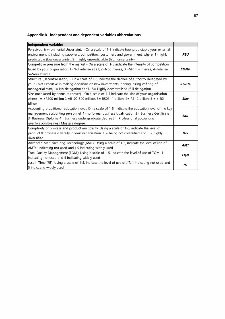
67
Appendix B –independent and dependent variables abbreviations
Independent variables
Perceived Environmental Uncertainty - On a scale of 1-5 indicate how predictable your external
environment is including suppliers, competitors, customers and government, where; 1=highly
predictable (low uncertainty), 5= highly unpredictable (high uncertainty)
PEU
Competitive pressure from the market - On a scale of 1-5 indicate the intensity of competition
faced by your organisation 1=Not intense at all, 2=Not intense, 3 =Slightly intense, 4=Intense,
5=Very Intense
COMP
Structure (Decentralisation) - On a scale of 1-5 indicate the degree of authority delegated by
your Chief Executive in making decisions on new investments, pricing, hiring & firing of
managerial staff, 1= No delegation at all, 5= Highly decentralised (full delegation
STRUC
Size (measured by annual turnover) - On a scale of 1-5 indicate the size of your organisation
where 1= <R100 million 2 =R100-500 million, 3= R501- 1 billion, 4= R1- 2 billion, 5 = > R2
billion
Size
Accounting practitioner education level: On a scale of 1-5, indicate the education level of the key
management accounting personnel: 1=no formal business qualification 2= Business Certificate
3=Business Diploma 4= Business undergraduate degree5 = Professional accounting
qualification/Business Masters degree
Edu
Complexity of process and product multiplicity: Using a scale of 1-5, indicate the level of
product & process diversity in your organisation, 1 = being not diversified and 5 = highly
diversified
Div
Advanced Manufacturing Technology (AMT): Using a scale of 1-5, indicate the level of use of
AMT;1 indicating not used and >5 indicating widely usedAMT
Total Quality Management (TQM); Using a scale of 1-5, indicate the level of use of TQM, 1
indicating not used and 5 indicating widely usedTQM
Just In Time (JIT); Using a scale of 1-5, indicate the level of use of JIT, 1 indicating not used and
5 indicating widely used JIT
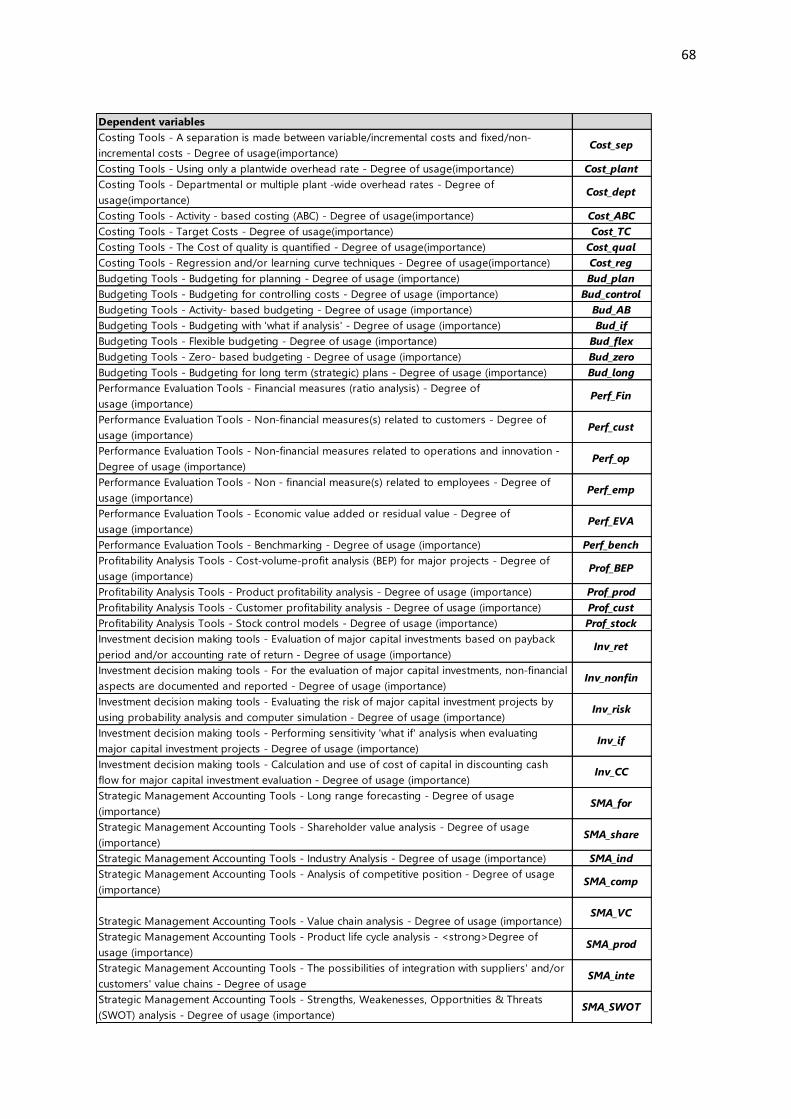
68
Dependent variables
Costing Tools - A separation is made between variable/incremental costs and fixed/non-
incremental costs - Degree of usage(importance)Cost_sep
Costing Tools - Using only a plantwide overhead rate - Degree of usage(importance) Cost_plant
Costing Tools - Departmental or multiple plant -wide overhead rates - Degree of
usage(importance)Cost_dept
Costing Tools - Activity - based costing (ABC) - Degree of usage(importance) Cost_ABC
Costing Tools - Target Costs - Degree of usage(importance) Cost_TC
Costing Tools - The Cost of quality is quantified - Degree of usage(importance) Cost_qual
Costing Tools - Regression and/or learning curve techniques - Degree of usage(importance) Cost_reg
Budgeting Tools - Budgeting for planning - Degree of usage (importance) Bud_plan
Budgeting Tools - Budgeting for controlling costs - Degree of usage (importance) Bud_control
Budgeting Tools - Activity- based budgeting - Degree of usage (importance) Bud_AB
Budgeting Tools - Budgeting with 'what if analysis' - Degree of usage (importance) Bud_if
Budgeting Tools - Flexible budgeting - Degree of usage (importance) Bud_flex
Budgeting Tools - Zero- based budgeting - Degree of usage (importance) Bud_zero
Budgeting Tools - Budgeting for long term (strategic) plans - Degree of usage (importance) Bud_long
Performance Evaluation Tools - Financial measures (ratio analysis) - Degree of
usage (importance)Perf_Fin
Performance Evaluation Tools - Non-financial measures(s) related to customers - Degree of
usage (importance)Perf_cust
Performance Evaluation Tools - Non-financial measures related to operations and innovation -
Degree of usage (importance)Perf_op
Performance Evaluation Tools - Non - financial measure(s) related to employees - Degree of
usage (importance)Perf_emp
Performance Evaluation Tools - Economic value added or residual value - Degree of
usage (importance)Perf_EVA
Performance Evaluation Tools - Benchmarking - Degree of usage (importance) Perf_bench
Profitability Analysis Tools - Cost-volume-profit analysis (BEP) for major projects - Degree of
usage (importance)Prof_BEP
Profitability Analysis Tools - Product profitability analysis - Degree of usage (importance) Prof_prod
Profitability Analysis Tools - Customer profitability analysis - Degree of usage (importance) Prof_cust
Profitability Analysis Tools - Stock control models - Degree of usage (importance) Prof_stock
Investment decision making tools - Evaluation of major capital investments based on payback
period and/or accounting rate of return - Degree of usage (importance)Inv_ret
Investment decision making tools - For the evaluation of major capital investments, non-financial
aspects are documented and reported - Degree of usage (importance)Inv_nonfin
Investment decision making tools - Evaluating the risk of major capital investment projects by
using probability analysis and computer simulation - Degree of usage (importance)Inv_risk
Investment decision making tools - Performing sensitivity 'what if' analysis when evaluating
major capital investment projects - Degree of usage (importance)Inv_if
Investment decision making tools - Calculation and use of cost of capital in discounting cash
flow for major capital investment evaluation - Degree of usage (importance)Inv_CC
Strategic Management Accounting Tools - Long range forecasting - Degree of usage
(importance)SMA_for
Strategic Management Accounting Tools - Shareholder value analysis - Degree of usage
(importance)SMA_share
Strategic Management Accounting Tools - Industry Analysis - Degree of usage (importance) SMA_ind
Strategic Management Accounting Tools - Analysis of competitive position - Degree of usage
(importance)SMA_comp
Strategic Management Accounting Tools - Value chain analysis - Degree of usage (importance)SMA_VC
Strategic Management Accounting Tools - Product life cycle analysis - <strong>Degree of
usage (importance)SMA_prod
Strategic Management Accounting Tools - The possibilities of integration with suppliers' and/or
customers' value chains - Degree of usageSMA_inte
Strategic Management Accounting Tools - Strengths, Weakenesses, Opportnities & Threats
(SWOT) analysis - Degree of usage (importance)SMA_SWOT
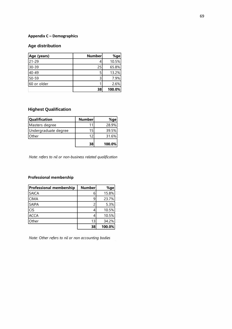
69
Appendix C – Demographics
Age distribution
Age (years) Number %ge
21-29 4 10.5%
30-39 25 65.8%
40-49 5 13.2%
50-59 3 7.9%
60 or older 1 2.6%
38 100.0%
Highest Qualification
Qualification Number %ge
Masters degree 11 28.9%
Undergraduate degree 15 39.5%
Other 12 31.6%
38 100.0%
Note: refers to nil or non-business related qualification
Professional membership
Professional membership Number %ge
SAICA 6 15.8%
CIMA 9 23.7%
SAIPA 2 5.3%
CIS 4 10.5%
ACCA 4 10.5%
Other 13 34.2%
38 100.0%
Note: Other refers to nil or non accounting bodies
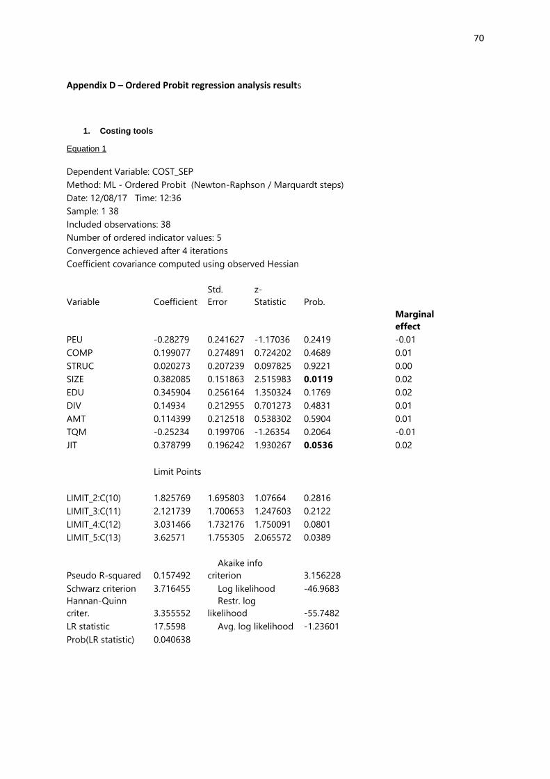
70
Appendix D – Ordered Probit regression analysis results
1. Costing tools
Equation 1
Dependent Variable: COST_SEP
Method: ML - Ordered Probit (Newton-Raphson / Marquardt steps)
Date: 12/08/17 Time: 12:36
Sample: 1 38
Included observations: 38
Number of ordered indicator values: 5
Convergence achieved after 4 iterations
Coefficient covariance computed using observed Hessian
Variable Coefficient
Std.
Error
z-
Statistic Prob.
Marginal
effect
PEU -0.28279 0.241627 -1.17036 0.2419
-0.01
COMP 0.199077 0.274891 0.724202 0.4689
0.01
STRUC 0.020273 0.207239 0.097825 0.9221
0.00
SIZE 0.382085 0.151863 2.515983 0.0119
0.02
EDU 0.345904 0.256164 1.350324 0.1769
0.02
DIV 0.14934 0.212955 0.701273 0.4831
0.01
AMT 0.114399 0.212518 0.538302 0.5904
0.01
TQM -0.25234 0.199706 -1.26354 0.2064
-0.01
JIT 0.378799 0.196242 1.930267 0.0536
0.02
Limit Points
LIMIT_2:C(10) 1.825769 1.695803 1.07664 0.2816
LIMIT_3:C(11) 2.121739 1.700653 1.247603 0.2122
LIMIT_4:C(12) 3.031466 1.732176 1.750091 0.0801
LIMIT_5:C(13) 3.62571 1.755305 2.065572 0.0389
Pseudo R-squared 0.157492
Akaike info
criterion 3.156228
Schwarz criterion 3.716455 Log likelihood -46.9683
Hannan-Quinn
criter. 3.355552
Restr. log
likelihood -55.7482
LR statistic 17.5598 Avg. log likelihood -1.23601
Prob(LR statistic) 0.040638
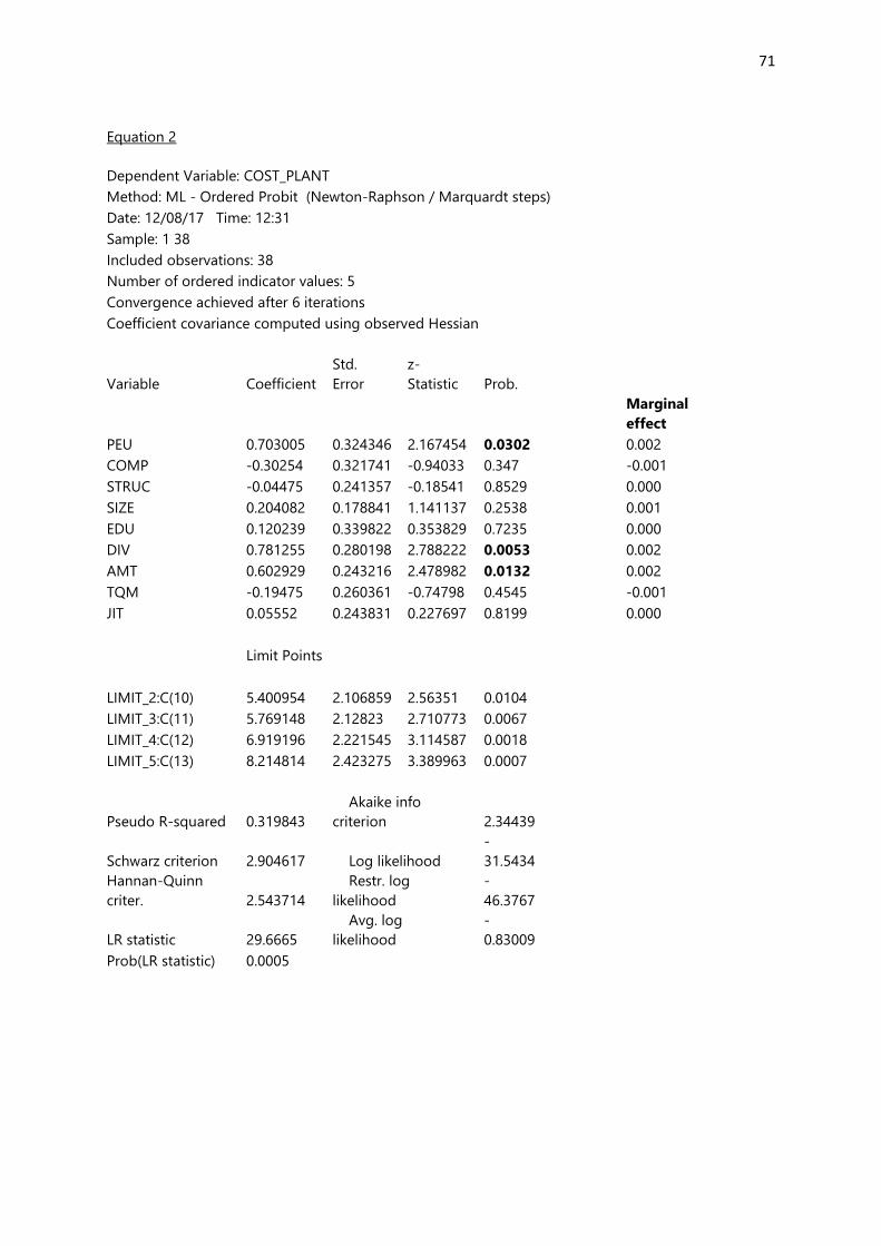
71
Equation 2
Dependent Variable: COST_PLANT
Method: ML - Ordered Probit (Newton-Raphson / Marquardt steps)
Date: 12/08/17 Time: 12:31
Sample: 1 38
Included observations: 38
Number of ordered indicator values: 5
Convergence achieved after 6 iterations
Coefficient covariance computed using observed Hessian
Variable Coefficient
Std.
Error
z-
Statistic Prob.
Marginal
effect
PEU 0.703005 0.324346 2.167454 0.0302
0.002
COMP -0.30254 0.321741 -0.94033 0.347
-0.001
STRUC -0.04475 0.241357 -0.18541 0.8529
0.000
SIZE 0.204082 0.178841 1.141137 0.2538
0.001
EDU 0.120239 0.339822 0.353829 0.7235
0.000
DIV 0.781255 0.280198 2.788222 0.0053
0.002
AMT 0.602929 0.243216 2.478982 0.0132
0.002
TQM -0.19475 0.260361 -0.74798 0.4545
-0.001
JIT 0.05552 0.243831 0.227697 0.8199
0.000
Limit Points
LIMIT_2:C(10) 5.400954 2.106859 2.56351 0.0104
LIMIT_3:C(11) 5.769148 2.12823 2.710773 0.0067
LIMIT_4:C(12) 6.919196 2.221545 3.114587 0.0018
LIMIT_5:C(13) 8.214814 2.423275 3.389963 0.0007
Pseudo R-squared 0.319843
Akaike info
criterion 2.34439
Schwarz criterion 2.904617 Log likelihood
-
31.5434
Hannan-Quinn
criter. 2.543714
Restr. log
likelihood
-
46.3767
LR statistic 29.6665
Avg. log
likelihood
-
0.83009
Prob(LR statistic) 0.0005
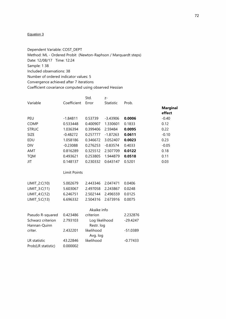
72
Equation 3
Dependent Variable: COST_DEPT
Method: ML - Ordered Probit (Newton-Raphson / Marquardt steps)
Date: 12/08/17 Time: 12:24
Sample: 1 38
Included observations: 38
Number of ordered indicator values: 5
Convergence achieved after 7 iterations
Coefficient covariance computed using observed Hessian
Variable Coefficient
Std.
Error
z-
Statistic Prob.
Marginal
effect
PEU -1.84811 0.53739 -3.43906 0.0006
-0.40
COMP 0.533448 0.400907 1.330601 0.1833
0.12
STRUC 1.036394 0.399406 2.59484 0.0095
0.22
SIZE -0.48272 0.257777 -1.87263 0.0611
-0.10
EDU 1.058186 0.346672 3.052407 0.0023
0.23
DIV -0.23088 0.276253 -0.83574 0.4033
-0.05
AMT 0.816289 0.325512 2.507709 0.0122
0.18
TQM 0.493621 0.253805 1.944879 0.0518
0.11
JIT 0.148137 0.230332 0.643147 0.5201
0.03
Limit Points
LIMIT_2:C(10) 5.002679 2.443346 2.047471 0.0406
LIMIT_3:C(11) 5.603067 2.497058 2.243867 0.0248
LIMIT_4:C(12) 6.246751 2.502144 2.496559 0.0125
LIMIT_5:C(13) 6.696332 2.504316 2.673916 0.0075
Pseudo R-squared 0.423486
Akaike info
criterion 2.232876
Schwarz criterion 2.793103 Log likelihood -29.4247
Hannan-Quinn
criter. 2.432201
Restr. log
likelihood -51.0389
LR statistic 43.22846
Avg. log
likelihood -0.77433
Prob(LR statistic) 0.000002
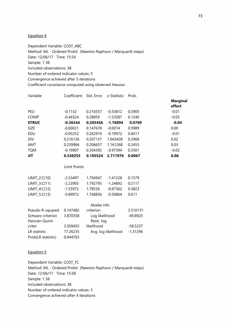
73
Equation 4
Dependent Variable: COST_ABC
Method: ML - Ordered Probit (Newton-Raphson / Marquardt steps)
Date: 12/06/17 Time: 15:54
Sample: 1 38
Included observations: 38
Number of ordered indicator values: 5
Convergence achieved after 5 iterations
Coefficient covariance computed using observed Hessian
Variable Coefficient Std. Error z-Statistic Prob.
Marginal
effect
PEU -0.1132 0.210357 -0.53812 0.5905
-0.01
COMP -0.44324 0.28859 -1.53587 0.1246
-0.05
STRUC -0.36344 0.205456 -1.76894 0.0769
-0.04
SIZE -0.00021 0.147678 -0.0014 0.9989
0.00
EDU -0.05252 0.262974 -0.19972 0.8417
-0.01
DIV 0.216126 0.207131 1.043428 0.2968
0.02
AMT 0.239984 0.206657 1.161268 0.2455
0.03
TQM -0.19907 0.204392 -0.97394 0.3301
-0.02
JIT 0.530255 0.195524 2.711976 0.0067
0.06
Limit Points
LIMIT_2:C(10) -2.53497 1.794947 -1.41228 0.1579
LIMIT_3:C(11) -2.23905 1.792795 -1.24892 0.2117
LIMIT_4:C(12) -1.55972 1.78536 -0.87362 0.3823
LIMIT_5:C(13) -0.89972 1.768856 -0.50864 0.611
Pseudo R-squared 0.147482
Akaike info
criterion 3.310131
Schwarz criterion 3.870358 Log likelihood -49.8925
Hannan-Quinn
criter. 3.509455
Restr. log
likelihood -58.5237
LR statistic 17.26235 Avg. log likelihood -1.31296
Prob(LR statistic) 0.044763
Equation 5
Dependent Variable: COST_TC
Method: ML - Ordered Probit (Newton-Raphson / Marquardt steps)
Date: 12/06/17 Time: 15:58
Sample: 1 38
Included observations: 38
Number of ordered indicator values: 5
Convergence achieved after 4 iterations
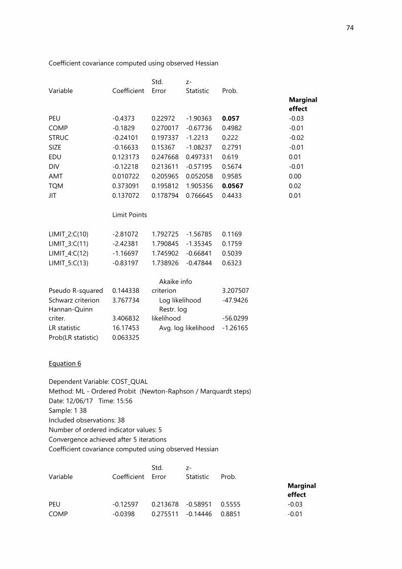
74
Coefficient covariance computed using observed Hessian
Variable Coefficient
Std.
Error
z-
Statistic Prob.
Marginal
effect
PEU -0.4373 0.22972 -1.90363 0.057
-0.03
COMP -0.1829 0.270017 -0.67736 0.4982
-0.01
STRUC -0.24101 0.197337 -1.2213 0.222
-0.02
SIZE -0.16633 0.15367 -1.08237 0.2791
-0.01
EDU 0.123173 0.247668 0.497331 0.619
0.01
DIV -0.12218 0.213611 -0.57195 0.5674
-0.01
AMT 0.010722 0.205965 0.052058 0.9585
0.00
TQM 0.373091 0.195812 1.905356 0.0567
0.02
JIT 0.137072 0.178794 0.766645 0.4433
0.01
Limit Points
LIMIT_2:C(10) -2.81072 1.792725 -1.56785 0.1169
LIMIT_3:C(11) -2.42381 1.790845 -1.35345 0.1759
LIMIT_4:C(12) -1.16697 1.745902 -0.66841 0.5039
LIMIT_5:C(13) -0.83197 1.738926 -0.47844 0.6323
Pseudo R-squared 0.144338
Akaike info
criterion 3.207507
Schwarz criterion 3.767734 Log likelihood -47.9426
Hannan-Quinn
criter. 3.406832
Restr. log
likelihood -56.0299
LR statistic 16.17453 Avg. log likelihood -1.26165
Prob(LR statistic) 0.063325
Equation 6
Dependent Variable: COST_QUAL
Method: ML - Ordered Probit (Newton-Raphson / Marquardt steps)
Date: 12/06/17 Time: 15:56
Sample: 1 38
Included observations: 38
Number of ordered indicator values: 5
Convergence achieved after 5 iterations
Coefficient covariance computed using observed Hessian
Variable Coefficient
Std.
Error
z-
Statistic Prob.
Marginal
effect
PEU -0.12597 0.213678 -0.58951 0.5555
-0.03
COMP -0.0398 0.275511 -0.14446 0.8851
-0.01
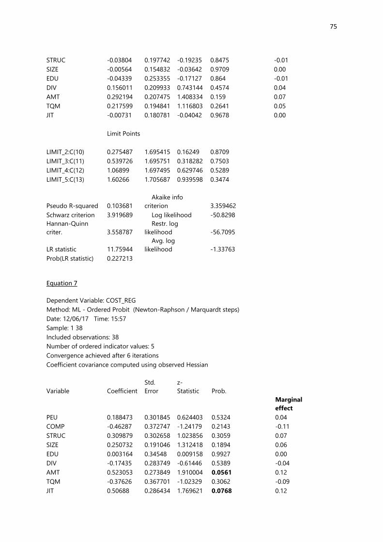
75
STRUC -0.03804 0.197742 -0.19235 0.8475
-0.01
SIZE -0.00564 0.154832 -0.03642 0.9709
0.00
EDU -0.04339 0.253355 -0.17127 0.864
-0.01
DIV 0.156011 0.209933 0.743144 0.4574
0.04
AMT 0.292194 0.207475 1.408334 0.159
0.07
TQM 0.217599 0.194841 1.116803 0.2641
0.05
JIT -0.00731 0.180781 -0.04042 0.9678
0.00
Limit Points
LIMIT_2:C(10) 0.275487 1.695415 0.16249 0.8709
LIMIT_3:C(11) 0.539726 1.695751 0.318282 0.7503
LIMIT_4:C(12) 1.06899 1.697495 0.629746 0.5289
LIMIT_5:C(13) 1.60266 1.705687 0.939598 0.3474
Pseudo R-squared 0.103681
Akaike info
criterion 3.359462
Schwarz criterion 3.919689 Log likelihood -50.8298
Hannan-Quinn
criter. 3.558787
Restr. log
likelihood -56.7095
LR statistic 11.75944
Avg. log
likelihood -1.33763
Prob(LR statistic) 0.227213
Equation 7
Dependent Variable: COST_REG
Method: ML - Ordered Probit (Newton-Raphson / Marquardt steps)
Date: 12/06/17 Time: 15:57
Sample: 1 38
Included observations: 38
Number of ordered indicator values: 5
Convergence achieved after 6 iterations
Coefficient covariance computed using observed Hessian
Variable Coefficient
Std.
Error
z-
Statistic Prob.
Marginal
effect
PEU 0.188473 0.301845 0.624403 0.5324
0.04
COMP -0.46287 0.372747 -1.24179 0.2143
-0.11
STRUC 0.309879 0.302658 1.023856 0.3059
0.07
SIZE 0.250732 0.191046 1.312418 0.1894
0.06
EDU 0.003164 0.34548 0.009158 0.9927
0.00
DIV -0.17435 0.283749 -0.61446 0.5389
-0.04
AMT 0.523053 0.273849 1.910004 0.0561
0.12
TQM -0.37626 0.367701 -1.02329 0.3062
-0.09
JIT 0.50688 0.286434 1.769621 0.0768
0.12
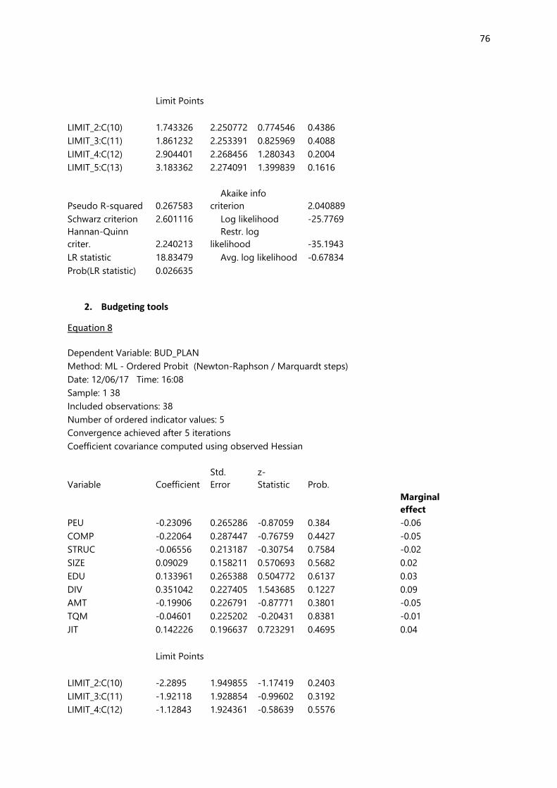
76
Limit Points
LIMIT_2:C(10) 1.743326 2.250772 0.774546 0.4386
LIMIT_3:C(11) 1.861232 2.253391 0.825969 0.4088
LIMIT_4:C(12) 2.904401 2.268456 1.280343 0.2004
LIMIT_5:C(13) 3.183362 2.274091 1.399839 0.1616
Pseudo R-squared 0.267583
Akaike info
criterion 2.040889
Schwarz criterion 2.601116 Log likelihood -25.7769
Hannan-Quinn
criter. 2.240213
Restr. log
likelihood -35.1943
LR statistic 18.83479 Avg. log likelihood -0.67834
Prob(LR statistic) 0.026635
2. Budgeting tools
Equation 8
Dependent Variable: BUD_PLAN
Method: ML - Ordered Probit (Newton-Raphson / Marquardt steps)
Date: 12/06/17 Time: 16:08
Sample: 1 38
Included observations: 38
Number of ordered indicator values: 5
Convergence achieved after 5 iterations
Coefficient covariance computed using observed Hessian
Variable Coefficient
Std.
Error
z-
Statistic Prob.
Marginal
effect
PEU -0.23096 0.265286 -0.87059 0.384
-0.06
COMP -0.22064 0.287447 -0.76759 0.4427
-0.05
STRUC -0.06556 0.213187 -0.30754 0.7584
-0.02
SIZE 0.09029 0.158211 0.570693 0.5682
0.02
EDU 0.133961 0.265388 0.504772 0.6137
0.03
DIV 0.351042 0.227405 1.543685 0.1227
0.09
AMT -0.19906 0.226791 -0.87771 0.3801
-0.05
TQM -0.04601 0.225202 -0.20431 0.8381
-0.01
JIT 0.142226 0.196637 0.723291 0.4695
0.04
Limit Points
LIMIT_2:C(10) -2.2895 1.949855 -1.17419 0.2403
LIMIT_3:C(11) -1.92118 1.928854 -0.99602 0.3192
LIMIT_4:C(12) -1.12843 1.924361 -0.58639 0.5576
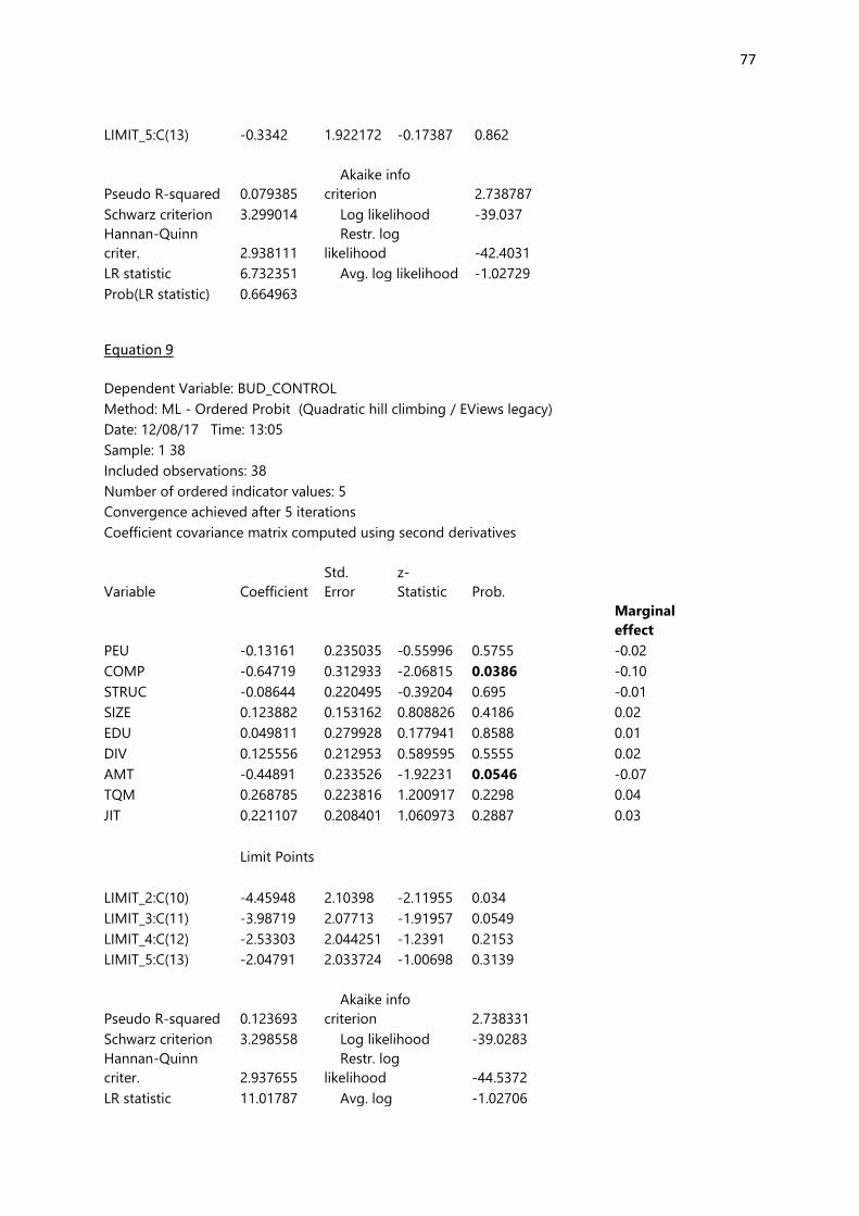
77
LIMIT_5:C(13) -0.3342 1.922172 -0.17387 0.862
Pseudo R-squared 0.079385
Akaike info
criterion 2.738787
Schwarz criterion 3.299014 Log likelihood -39.037
Hannan-Quinn
criter. 2.938111
Restr. log
likelihood -42.4031
LR statistic 6.732351 Avg. log likelihood -1.02729
Prob(LR statistic) 0.664963
Equation 9
Dependent Variable: BUD_CONTROL
Method: ML - Ordered Probit (Quadratic hill climbing / EViews legacy)
Date: 12/08/17 Time: 13:05
Sample: 1 38
Included observations: 38
Number of ordered indicator values: 5
Convergence achieved after 5 iterations
Coefficient covariance matrix computed using second derivatives
Variable Coefficient
Std.
Error
z-
Statistic Prob.
Marginal
effect
PEU -0.13161 0.235035 -0.55996 0.5755
-0.02
COMP -0.64719 0.312933 -2.06815 0.0386
-0.10
STRUC -0.08644 0.220495 -0.39204 0.695
-0.01
SIZE 0.123882 0.153162 0.808826 0.4186
0.02
EDU 0.049811 0.279928 0.177941 0.8588
0.01
DIV 0.125556 0.212953 0.589595 0.5555
0.02
AMT -0.44891 0.233526 -1.92231 0.0546
-0.07
TQM 0.268785 0.223816 1.200917 0.2298
0.04
JIT 0.221107 0.208401 1.060973 0.2887
0.03
Limit Points
LIMIT_2:C(10) -4.45948 2.10398 -2.11955 0.034
LIMIT_3:C(11) -3.98719 2.07713 -1.91957 0.0549
LIMIT_4:C(12) -2.53303 2.044251 -1.2391 0.2153
LIMIT_5:C(13) -2.04791 2.033724 -1.00698 0.3139
Pseudo R-squared 0.123693
Akaike info
criterion 2.738331
Schwarz criterion 3.298558 Log likelihood -39.0283
Hannan-Quinn
criter. 2.937655
Restr. log
likelihood -44.5372
LR statistic 11.01787 Avg. log -1.02706
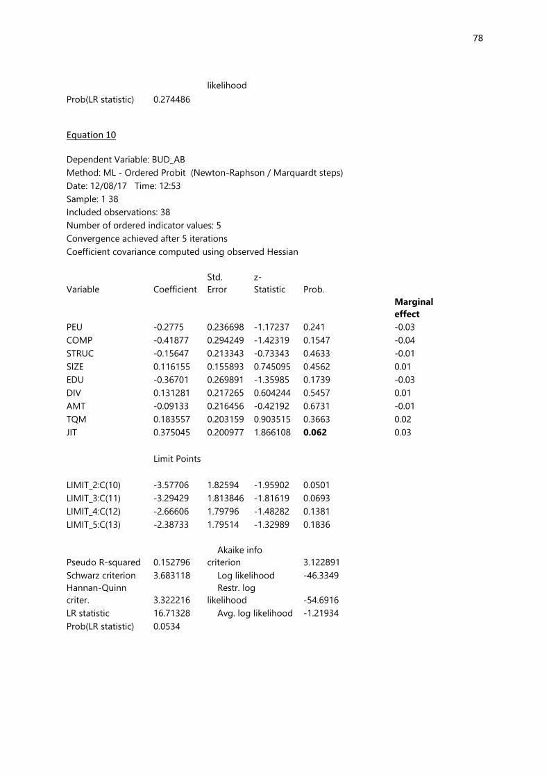
78
likelihood
Prob(LR statistic) 0.274486
Equation 10
Dependent Variable: BUD_AB
Method: ML - Ordered Probit (Newton-Raphson / Marquardt steps)
Date: 12/08/17 Time: 12:53
Sample: 1 38
Included observations: 38
Number of ordered indicator values: 5
Convergence achieved after 5 iterations
Coefficient covariance computed using observed Hessian
Variable Coefficient
Std.
Error
z-
Statistic Prob.
Marginal
effect
PEU -0.2775 0.236698 -1.17237 0.241
-0.03
COMP -0.41877 0.294249 -1.42319 0.1547
-0.04
STRUC -0.15647 0.213343 -0.73343 0.4633
-0.01
SIZE 0.116155 0.155893 0.745095 0.4562
0.01
EDU -0.36701 0.269891 -1.35985 0.1739
-0.03
DIV 0.131281 0.217265 0.604244 0.5457
0.01
AMT -0.09133 0.216456 -0.42192 0.6731
-0.01
TQM 0.183557 0.203159 0.903515 0.3663
0.02
JIT 0.375045 0.200977 1.866108 0.062
0.03
Limit Points
LIMIT_2:C(10) -3.57706 1.82594 -1.95902 0.0501
LIMIT_3:C(11) -3.29429 1.813846 -1.81619 0.0693
LIMIT_4:C(12) -2.66606 1.79796 -1.48282 0.1381
LIMIT_5:C(13) -2.38733 1.79514 -1.32989 0.1836
Pseudo R-squared 0.152796
Akaike info
criterion 3.122891
Schwarz criterion 3.683118 Log likelihood -46.3349
Hannan-Quinn
criter. 3.322216
Restr. log
likelihood -54.6916
LR statistic 16.71328 Avg. log likelihood -1.21934
Prob(LR statistic) 0.0534
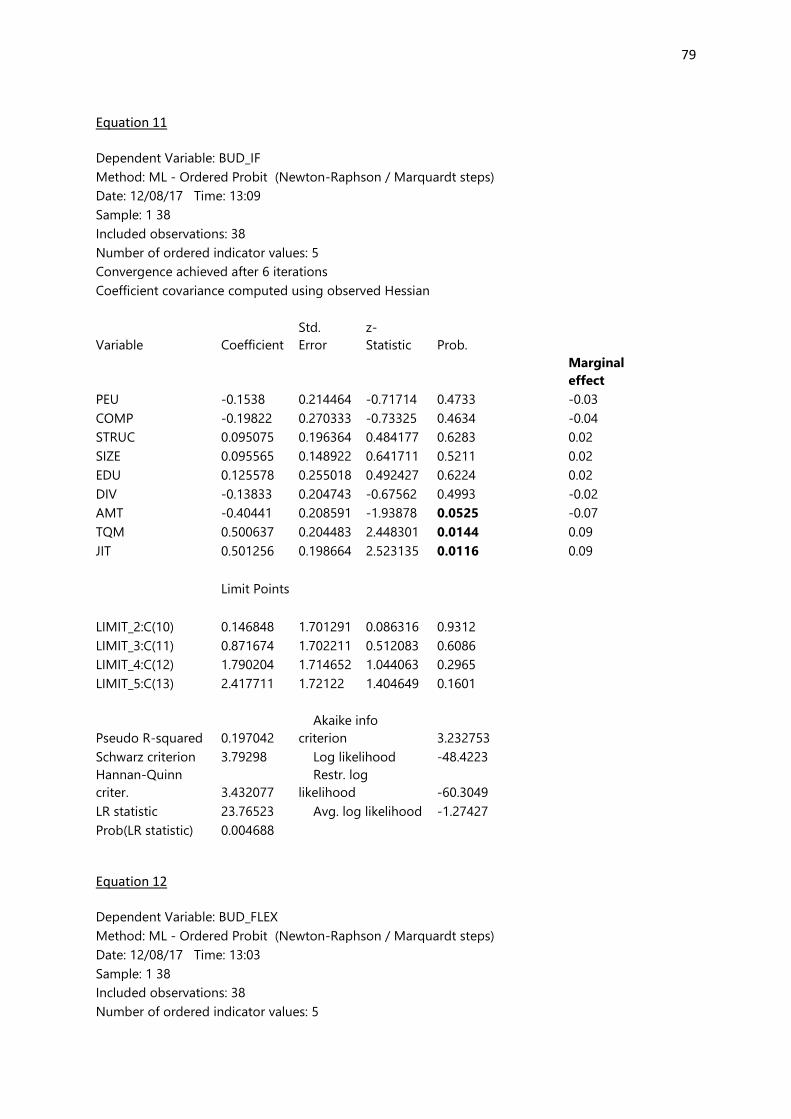
79
Equation 11
Dependent Variable: BUD_IF
Method: ML - Ordered Probit (Newton-Raphson / Marquardt steps)
Date: 12/08/17 Time: 13:09
Sample: 1 38
Included observations: 38
Number of ordered indicator values: 5
Convergence achieved after 6 iterations
Coefficient covariance computed using observed Hessian
Variable Coefficient
Std.
Error
z-
Statistic Prob.
Marginal
effect
PEU -0.1538 0.214464 -0.71714 0.4733
-0.03
COMP -0.19822 0.270333 -0.73325 0.4634
-0.04
STRUC 0.095075 0.196364 0.484177 0.6283
0.02
SIZE 0.095565 0.148922 0.641711 0.5211
0.02
EDU 0.125578 0.255018 0.492427 0.6224
0.02
DIV -0.13833 0.204743 -0.67562 0.4993
-0.02
AMT -0.40441 0.208591 -1.93878 0.0525
-0.07
TQM 0.500637 0.204483 2.448301 0.0144
0.09
JIT 0.501256 0.198664 2.523135 0.0116
0.09
Limit Points
LIMIT_2:C(10) 0.146848 1.701291 0.086316 0.9312
LIMIT_3:C(11) 0.871674 1.702211 0.512083 0.6086
LIMIT_4:C(12) 1.790204 1.714652 1.044063 0.2965
LIMIT_5:C(13) 2.417711 1.72122 1.404649 0.1601
Pseudo R-squared 0.197042
Akaike info
criterion 3.232753
Schwarz criterion 3.79298 Log likelihood -48.4223
Hannan-Quinn
criter. 3.432077
Restr. log
likelihood -60.3049
LR statistic 23.76523 Avg. log likelihood -1.27427
Prob(LR statistic) 0.004688
Equation 12
Dependent Variable: BUD_FLEX
Method: ML - Ordered Probit (Newton-Raphson / Marquardt steps)
Date: 12/08/17 Time: 13:03
Sample: 1 38
Included observations: 38
Number of ordered indicator values: 5
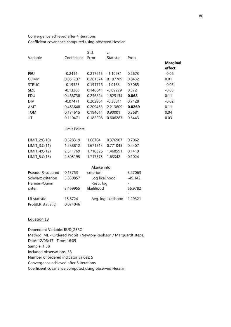
80
Convergence achieved after 4 iterations
Coefficient covariance computed using observed Hessian
Variable Coefficient
Std.
Error
z-
Statistic Prob.
Marginal
effect
PEU -0.2414 0.217615 -1.10931 0.2673
-0.06
COMP 0.051737 0.261574 0.197789 0.8432
0.01
STRUC -0.19523 0.191716 -1.0183 0.3085
-0.05
SIZE -0.13288 0.148841 -0.89279 0.372
-0.03
EDU 0.468738 0.256824 1.825134 0.068
0.11
DIV -0.07471 0.202964 -0.36811 0.7128
-0.02
AMT 0.463648 0.209453 2.213609 0.0269
0.11
TQM 0.174615 0.194014 0.90001 0.3681
0.04
JIT 0.110471 0.182208 0.606287 0.5443
0.03
Limit Points
LIMIT_2:C(10) 0.628319 1.66704 0.376907 0.7062
LIMIT_3:C(11) 1.288812 1.671513 0.771045 0.4407
LIMIT_4:C(12) 2.511769 1.710326 1.468591 0.1419
LIMIT_5:C(13) 2.805195 1.717375 1.63342 0.1024
Pseudo R-squared 0.13753
Akaike info
criterion 3.27063
Schwarz criterion 3.830857 Log likelihood -49.142
Hannan-Quinn
criter. 3.469955
Restr. log
likelihood
-
56.9782
LR statistic 15.6724 Avg. log likelihood
-
1.29321
Prob(LR statistic) 0.074046
Equation 13
Dependent Variable: BUD_ZERO
Method: ML - Ordered Probit (Newton-Raphson / Marquardt steps)
Date: 12/06/17 Time: 16:09
Sample: 1 38
Included observations: 38
Number of ordered indicator values: 5
Convergence achieved after 5 iterations
Coefficient covariance computed using observed Hessian
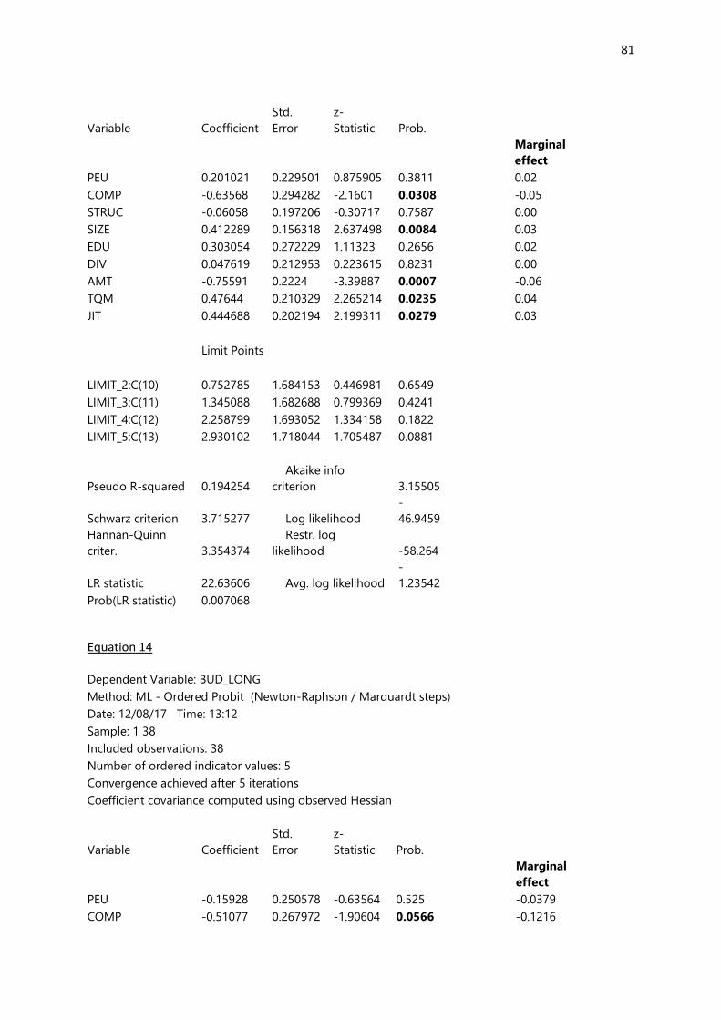
81
Variable Coefficient
Std.
Error
z-
Statistic Prob.
Marginal
effect
PEU 0.201021 0.229501 0.875905 0.3811
0.02
COMP -0.63568 0.294282 -2.1601 0.0308
-0.05
STRUC -0.06058 0.197206 -0.30717 0.7587
0.00
SIZE 0.412289 0.156318 2.637498 0.0084
0.03
EDU 0.303054 0.272229 1.11323 0.2656
0.02
DIV 0.047619 0.212953 0.223615 0.8231
0.00
AMT -0.75591 0.2224 -3.39887 0.0007
-0.06
TQM 0.47644 0.210329 2.265214 0.0235
0.04
JIT 0.444688 0.202194 2.199311 0.0279
0.03
Limit Points
LIMIT_2:C(10) 0.752785 1.684153 0.446981 0.6549
LIMIT_3:C(11) 1.345088 1.682688 0.799369 0.4241
LIMIT_4:C(12) 2.258799 1.693052 1.334158 0.1822
LIMIT_5:C(13) 2.930102 1.718044 1.705487 0.0881
Pseudo R-squared 0.194254
Akaike info
criterion 3.15505
Schwarz criterion 3.715277 Log likelihood
-
46.9459
Hannan-Quinn
criter. 3.354374
Restr. log
likelihood -58.264
LR statistic 22.63606 Avg. log likelihood
-
1.23542
Prob(LR statistic) 0.007068
Equation 14
Dependent Variable: BUD_LONG
Method: ML - Ordered Probit (Newton-Raphson / Marquardt steps)
Date: 12/08/17 Time: 13:12
Sample: 1 38
Included observations: 38
Number of ordered indicator values: 5
Convergence achieved after 5 iterations
Coefficient covariance computed using observed Hessian
Variable Coefficient
Std.
Error
z-
Statistic Prob.
Marginal
effect
PEU -0.15928 0.250578 -0.63564 0.525
-0.0379
COMP -0.51077 0.267972 -1.90604 0.0566
-0.1216
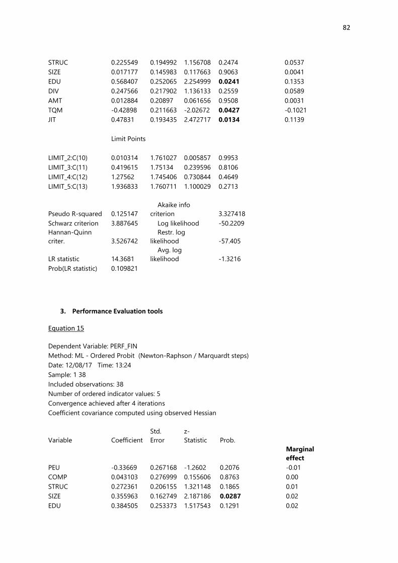
82
STRUC 0.225549 0.194992 1.156708 0.2474
0.0537
SIZE 0.017177 0.145983 0.117663 0.9063
0.0041
EDU 0.568407 0.252065 2.254999 0.0241
0.1353
DIV 0.247566 0.217902 1.136133 0.2559
0.0589
AMT 0.012884 0.20897 0.061656 0.9508
0.0031
TQM -0.42898 0.211663 -2.02672 0.0427
-0.1021
JIT 0.47831 0.193435 2.472717 0.0134
0.1139
Limit Points
LIMIT_2:C(10) 0.010314 1.761027 0.005857 0.9953
LIMIT_3:C(11) 0.419615 1.75134 0.239596 0.8106
LIMIT_4:C(12) 1.27562 1.745406 0.730844 0.4649
LIMIT_5:C(13) 1.936833 1.760711 1.100029 0.2713
Pseudo R-squared 0.125147
Akaike info
criterion 3.327418
Schwarz criterion 3.887645 Log likelihood -50.2209
Hannan-Quinn
criter. 3.526742
Restr. log
likelihood -57.405
LR statistic 14.3681
Avg. log
likelihood -1.3216
Prob(LR statistic) 0.109821
3. Performance Evaluation tools
Equation 15
Dependent Variable: PERF_FIN
Method: ML - Ordered Probit (Newton-Raphson / Marquardt steps)
Date: 12/08/17 Time: 13:24
Sample: 1 38
Included observations: 38
Number of ordered indicator values: 5
Convergence achieved after 4 iterations
Coefficient covariance computed using observed Hessian
Variable Coefficient
Std.
Error
z-
Statistic Prob.
Marginal
effect
PEU -0.33669 0.267168 -1.2602 0.2076
-0.01
COMP 0.043103 0.276999 0.155606 0.8763
0.00
STRUC 0.272361 0.206155 1.321148 0.1865
0.01
SIZE 0.355963 0.162749 2.187186 0.0287
0.02
EDU 0.384505 0.253373 1.517543 0.1291
0.02
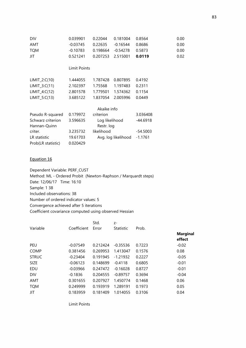
83
DIV 0.039901 0.22044 0.181004 0.8564
0.00
AMT -0.03745 0.22635 -0.16544 0.8686
0.00
TQM -0.10783 0.198664 -0.54278 0.5873
0.00
JIT 0.521241 0.207253 2.515001 0.0119
0.02
Limit Points
LIMIT_2:C(10) 1.444055 1.787428 0.807895 0.4192
LIMIT_3:C(11) 2.102397 1.75568 1.197483 0.2311
LIMIT_4:C(12) 2.801578 1.779501 1.574362 0.1154
LIMIT_5:C(13) 3.685122 1.837054 2.005996 0.0449
Pseudo R-squared 0.179972
Akaike info
criterion 3.036408
Schwarz criterion 3.596635 Log likelihood -44.6918
Hannan-Quinn
criter. 3.235732
Restr. log
likelihood -54.5003
LR statistic 19.61703 Avg. log likelihood -1.1761
Prob(LR statistic) 0.020429
Equation 16
Dependent Variable: PERF_CUST
Method: ML - Ordered Probit (Newton-Raphson / Marquardt steps)
Date: 12/06/17 Time: 16:10
Sample: 1 38
Included observations: 38
Number of ordered indicator values: 5
Convergence achieved after 5 iterations
Coefficient covariance computed using observed Hessian
Variable Coefficient
Std.
Error
z-
Statistic Prob.
Marginal
effect
PEU -0.07549 0.212424 -0.35536 0.7223
-0.02
COMP 0.381456 0.269953 1.413047 0.1576
0.08
STRUC -0.23404 0.191945 -1.21932 0.2227
-0.05
SIZE -0.06123 0.148699 -0.4118 0.6805
-0.01
EDU -0.03966 0.247472 -0.16028 0.8727
-0.01
DIV -0.1836 0.204555 -0.89757 0.3694
-0.04
AMT 0.301655 0.207927 1.450774 0.1468
0.06
TQM 0.249999 0.193919 1.289191 0.1973
0.05
JIT 0.183959 0.181409 1.014055 0.3106
0.04
Limit Points
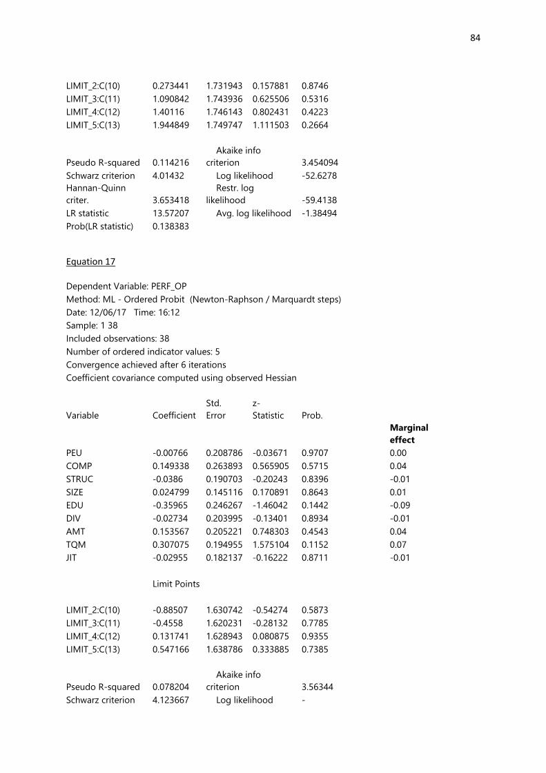
84
LIMIT_2:C(10) 0.273441 1.731943 0.157881 0.8746
LIMIT_3:C(11) 1.090842 1.743936 0.625506 0.5316
LIMIT_4:C(12) 1.40116 1.746143 0.802431 0.4223
LIMIT_5:C(13) 1.944849 1.749747 1.111503 0.2664
Pseudo R-squared 0.114216
Akaike info
criterion 3.454094
Schwarz criterion 4.01432 Log likelihood -52.6278
Hannan-Quinn
criter. 3.653418
Restr. log
likelihood -59.4138
LR statistic 13.57207 Avg. log likelihood -1.38494
Prob(LR statistic) 0.138383
Equation 17
Dependent Variable: PERF_OP
Method: ML - Ordered Probit (Newton-Raphson / Marquardt steps)
Date: 12/06/17 Time: 16:12
Sample: 1 38
Included observations: 38
Number of ordered indicator values: 5
Convergence achieved after 6 iterations
Coefficient covariance computed using observed Hessian
Variable Coefficient
Std.
Error
z-
Statistic Prob.
Marginal
effect
PEU -0.00766 0.208786 -0.03671 0.9707
0.00
COMP 0.149338 0.263893 0.565905 0.5715
0.04
STRUC -0.0386 0.190703 -0.20243 0.8396
-0.01
SIZE 0.024799 0.145116 0.170891 0.8643
0.01
EDU -0.35965 0.246267 -1.46042 0.1442
-0.09
DIV -0.02734 0.203995 -0.13401 0.8934
-0.01
AMT 0.153567 0.205221 0.748303 0.4543
0.04
TQM 0.307075 0.194955 1.575104 0.1152
0.07
JIT -0.02955 0.182137 -0.16222 0.8711
-0.01
Limit Points
LIMIT_2:C(10) -0.88507 1.630742 -0.54274 0.5873
LIMIT_3:C(11) -0.4558 1.620231 -0.28132 0.7785
LIMIT_4:C(12) 0.131741 1.628943 0.080875 0.9355
LIMIT_5:C(13) 0.547166 1.638786 0.333885 0.7385
Pseudo R-squared 0.078204
Akaike info
criterion 3.56344
Schwarz criterion 4.123667 Log likelihood -
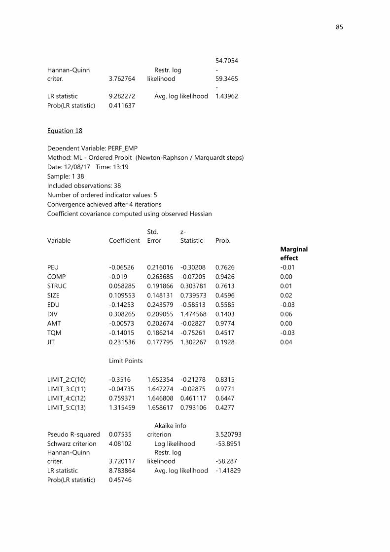
85
54.7054
Hannan-Quinn
criter. 3.762764
Restr. log
likelihood
-
59.3465
LR statistic 9.282272 Avg. log likelihood
-
1.43962
Prob(LR statistic) 0.411637
Equation 18
Dependent Variable: PERF_EMP
Method: ML - Ordered Probit (Newton-Raphson / Marquardt steps)
Date: 12/08/17 Time: 13:19
Sample: 1 38
Included observations: 38
Number of ordered indicator values: 5
Convergence achieved after 4 iterations
Coefficient covariance computed using observed Hessian
Variable Coefficient
Std.
Error
z-
Statistic Prob.
Marginal
effect
PEU -0.06526 0.216016 -0.30208 0.7626
-0.01
COMP -0.019 0.263685 -0.07205 0.9426
0.00
STRUC 0.058285 0.191866 0.303781 0.7613
0.01
SIZE 0.109553 0.148131 0.739573 0.4596
0.02
EDU -0.14253 0.243579 -0.58513 0.5585
-0.03
DIV 0.308265 0.209055 1.474568 0.1403
0.06
AMT -0.00573 0.202674 -0.02827 0.9774
0.00
TQM -0.14015 0.186214 -0.75261 0.4517
-0.03
JIT 0.231536 0.177795 1.302267 0.1928
0.04
Limit Points
LIMIT_2:C(10) -0.3516 1.652354 -0.21278 0.8315
LIMIT_3:C(11) -0.04735 1.647274 -0.02875 0.9771
LIMIT_4:C(12) 0.759371 1.646808 0.461117 0.6447
LIMIT_5:C(13) 1.315459 1.658617 0.793106 0.4277
Pseudo R-squared 0.07535
Akaike info
criterion 3.520793
Schwarz criterion 4.08102 Log likelihood -53.8951
Hannan-Quinn
criter. 3.720117
Restr. log
likelihood -58.287
LR statistic 8.783864 Avg. log likelihood -1.41829
Prob(LR statistic) 0.45746
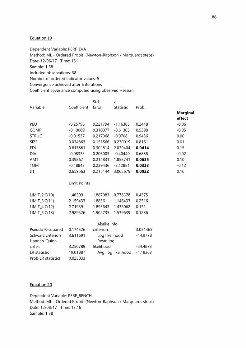
86
Equation 19
Dependent Variable: PERF_EVA
Method: ML - Ordered Probit (Newton-Raphson / Marquardt steps)
Date: 12/06/17 Time: 16:11
Sample: 1 38
Included observations: 38
Number of ordered indicator values: 5
Convergence achieved after 6 iterations
Coefficient covariance computed using observed Hessian
Variable Coefficient
Std.
Error
z-
Statistic Prob.
Marginal
effect
PEU -0.25796 0.221794 -1.16305 0.2448
-0.06
COMP -0.19009 0.310077 -0.61305 0.5398
-0.05
STRUC -0.01537 0.217068 -0.0708 0.9436
0.00
SIZE 0.034863 0.151566 0.230019 0.8181
0.01
EDU 0.617561 0.302814 2.039404 0.0414
0.15
DIV -0.08333 0.206003 -0.40449 0.6858
-0.02
AMT 0.39867 0.214831 1.855741 0.0635
0.10
TQM -0.48843 0.229436 -2.12881 0.0333
-0.12
JIT 0.659563 0.215144 3.065679 0.0022
0.16
Limit Points
LIMIT_2:C(10) 1.46509 1.887083 0.776378 0.4375
LIMIT_3:C(11) 2.159433 1.88361 1.146433 0.2516
LIMIT_4:C(12) 2.71939 1.893643 1.436062 0.151
LIMIT_5:C(13) 2.929526 1.902735 1.539639 0.1236
Pseudo R-squared 0.174526
Akaike info
criterion 3.051465
Schwarz criterion 3.611691 Log likelihood -44.9778
Hannan-Quinn
criter. 3.250789
Restr. log
likelihood -54.4873
LR statistic 19.01887 Avg. log likelihood -1.18363
Prob(LR statistic) 0.025033
Equation 20
Dependent Variable: PERF_BENCH
Method: ML - Ordered Probit (Newton-Raphson / Marquardt steps)
Date: 12/08/17 Time: 13:16
Sample: 1 38
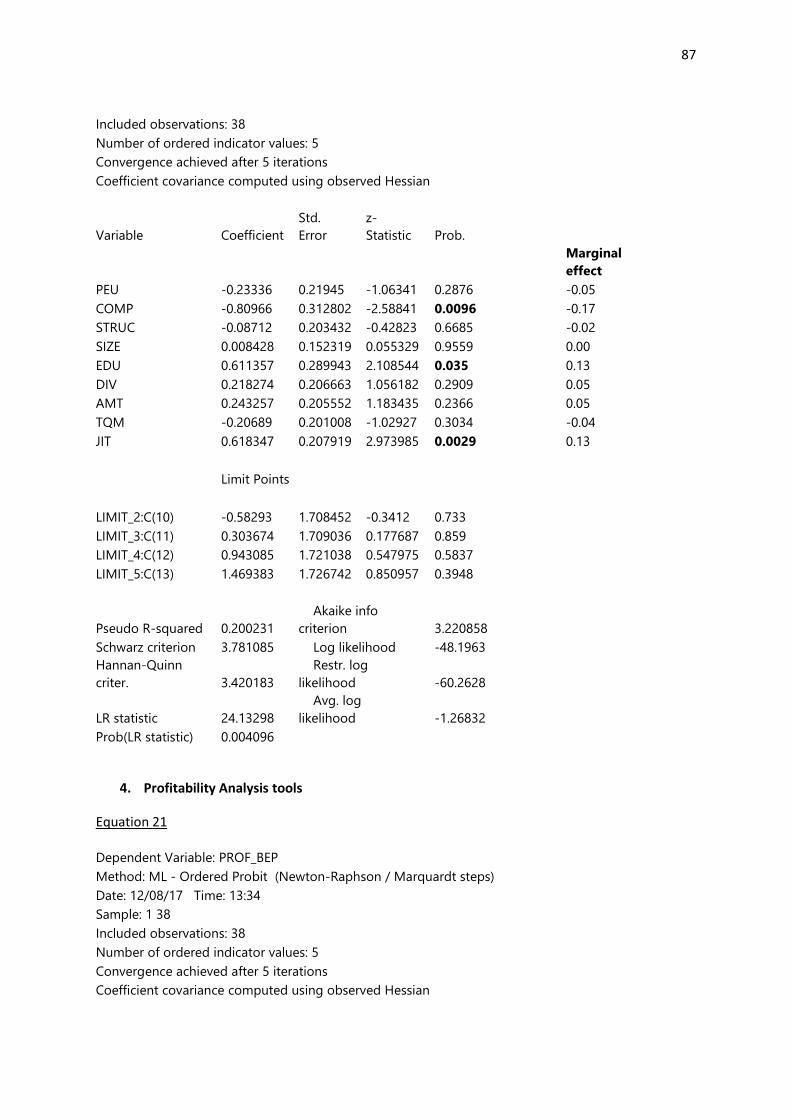
87
Included observations: 38
Number of ordered indicator values: 5
Convergence achieved after 5 iterations
Coefficient covariance computed using observed Hessian
Variable Coefficient
Std.
Error
z-
Statistic Prob.
Marginal
effect
PEU -0.23336 0.21945 -1.06341 0.2876
-0.05
COMP -0.80966 0.312802 -2.58841 0.0096
-0.17
STRUC -0.08712 0.203432 -0.42823 0.6685
-0.02
SIZE 0.008428 0.152319 0.055329 0.9559
0.00
EDU 0.611357 0.289943 2.108544 0.035
0.13
DIV 0.218274 0.206663 1.056182 0.2909
0.05
AMT 0.243257 0.205552 1.183435 0.2366
0.05
TQM -0.20689 0.201008 -1.02927 0.3034
-0.04
JIT 0.618347 0.207919 2.973985 0.0029
0.13
Limit Points
LIMIT_2:C(10) -0.58293 1.708452 -0.3412 0.733
LIMIT_3:C(11) 0.303674 1.709036 0.177687 0.859
LIMIT_4:C(12) 0.943085 1.721038 0.547975 0.5837
LIMIT_5:C(13) 1.469383 1.726742 0.850957 0.3948
Pseudo R-squared 0.200231
Akaike info
criterion 3.220858
Schwarz criterion 3.781085 Log likelihood -48.1963
Hannan-Quinn
criter. 3.420183
Restr. log
likelihood -60.2628
LR statistic 24.13298
Avg. log
likelihood -1.26832
Prob(LR statistic) 0.004096
4. Profitability Analysis tools
Equation 21
Dependent Variable: PROF_BEP
Method: ML - Ordered Probit (Newton-Raphson / Marquardt steps)
Date: 12/08/17 Time: 13:34
Sample: 1 38
Included observations: 38
Number of ordered indicator values: 5
Convergence achieved after 5 iterations
Coefficient covariance computed using observed Hessian
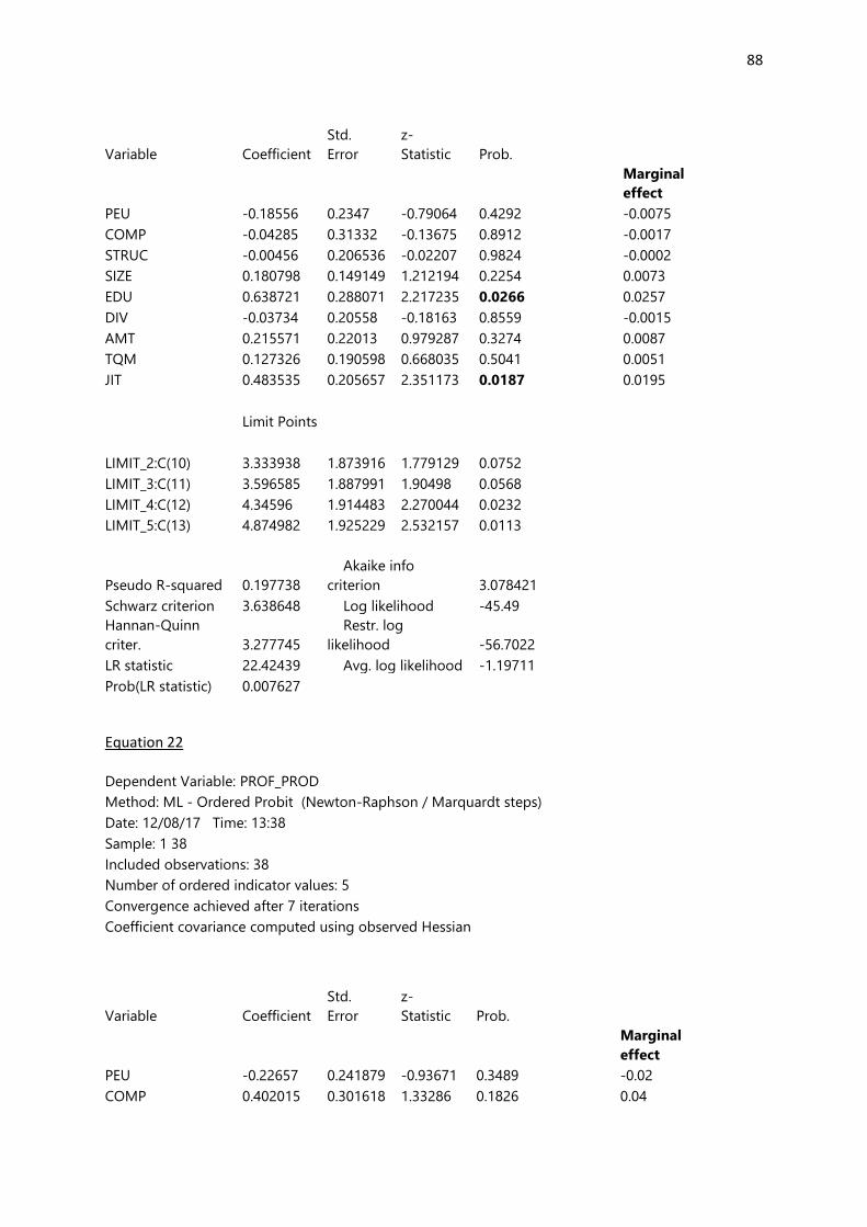
88
Variable Coefficient
Std.
Error
z-
Statistic Prob.
Marginal
effect
PEU -0.18556 0.2347 -0.79064 0.4292
-0.0075
COMP -0.04285 0.31332 -0.13675 0.8912
-0.0017
STRUC -0.00456 0.206536 -0.02207 0.9824
-0.0002
SIZE 0.180798 0.149149 1.212194 0.2254
0.0073
EDU 0.638721 0.288071 2.217235 0.0266
0.0257
DIV -0.03734 0.20558 -0.18163 0.8559
-0.0015
AMT 0.215571 0.22013 0.979287 0.3274
0.0087
TQM 0.127326 0.190598 0.668035 0.5041
0.0051
JIT 0.483535 0.205657 2.351173 0.0187
0.0195
Limit Points
LIMIT_2:C(10) 3.333938 1.873916 1.779129 0.0752
LIMIT_3:C(11) 3.596585 1.887991 1.90498 0.0568
LIMIT_4:C(12) 4.34596 1.914483 2.270044 0.0232
LIMIT_5:C(13) 4.874982 1.925229 2.532157 0.0113
Pseudo R-squared 0.197738
Akaike info
criterion 3.078421
Schwarz criterion 3.638648 Log likelihood -45.49
Hannan-Quinn
criter. 3.277745
Restr. log
likelihood -56.7022
LR statistic 22.42439 Avg. log likelihood -1.19711
Prob(LR statistic) 0.007627
Equation 22
Dependent Variable: PROF_PROD
Method: ML - Ordered Probit (Newton-Raphson / Marquardt steps)
Date: 12/08/17 Time: 13:38
Sample: 1 38
Included observations: 38
Number of ordered indicator values: 5
Convergence achieved after 7 iterations
Coefficient covariance computed using observed Hessian
Variable Coefficient
Std.
Error
z-
Statistic Prob.
Marginal
effect
PEU -0.22657 0.241879 -0.93671 0.3489
-0.02
COMP 0.402015 0.301618 1.33286 0.1826
0.04
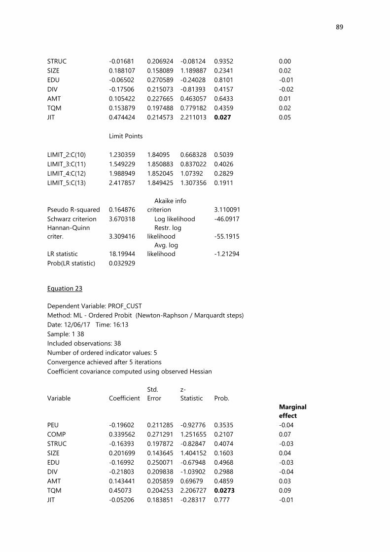
89
STRUC -0.01681 0.206924 -0.08124 0.9352
0.00
SIZE 0.188107 0.158089 1.189887 0.2341
0.02
EDU -0.06502 0.270589 -0.24028 0.8101
-0.01
DIV -0.17506 0.215073 -0.81393 0.4157
-0.02
AMT 0.105422 0.227665 0.463057 0.6433
0.01
TQM 0.153879 0.197488 0.779182 0.4359
0.02
JIT 0.474424 0.214573 2.211013 0.027
0.05
Limit Points
LIMIT_2:C(10) 1.230359 1.84095 0.668328 0.5039
LIMIT_3:C(11) 1.549229 1.850883 0.837022 0.4026
LIMIT_4:C(12) 1.988949 1.852045 1.07392 0.2829
LIMIT_5:C(13) 2.417857 1.849425 1.307356 0.1911
Pseudo R-squared 0.164876
Akaike info
criterion 3.110091
Schwarz criterion 3.670318 Log likelihood -46.0917
Hannan-Quinn
criter. 3.309416
Restr. log
likelihood -55.1915
LR statistic 18.19944
Avg. log
likelihood -1.21294
Prob(LR statistic) 0.032929
Equation 23
Dependent Variable: PROF_CUST
Method: ML - Ordered Probit (Newton-Raphson / Marquardt steps)
Date: 12/06/17 Time: 16:13
Sample: 1 38
Included observations: 38
Number of ordered indicator values: 5
Convergence achieved after 5 iterations
Coefficient covariance computed using observed Hessian
Variable Coefficient
Std.
Error
z-
Statistic Prob.
Marginal
effect
PEU -0.19602 0.211285 -0.92776 0.3535
-0.04
COMP 0.339562 0.271291 1.251655 0.2107
0.07
STRUC -0.16393 0.197872 -0.82847 0.4074
-0.03
SIZE 0.201699 0.143645 1.404152 0.1603
0.04
EDU -0.16992 0.250071 -0.67948 0.4968
-0.03
DIV -0.21803 0.209838 -1.03902 0.2988
-0.04
AMT 0.143441 0.205859 0.69679 0.4859
0.03
TQM 0.45073 0.204253 2.206727 0.0273
0.09
JIT -0.05206 0.183851 -0.28317 0.777
-0.01
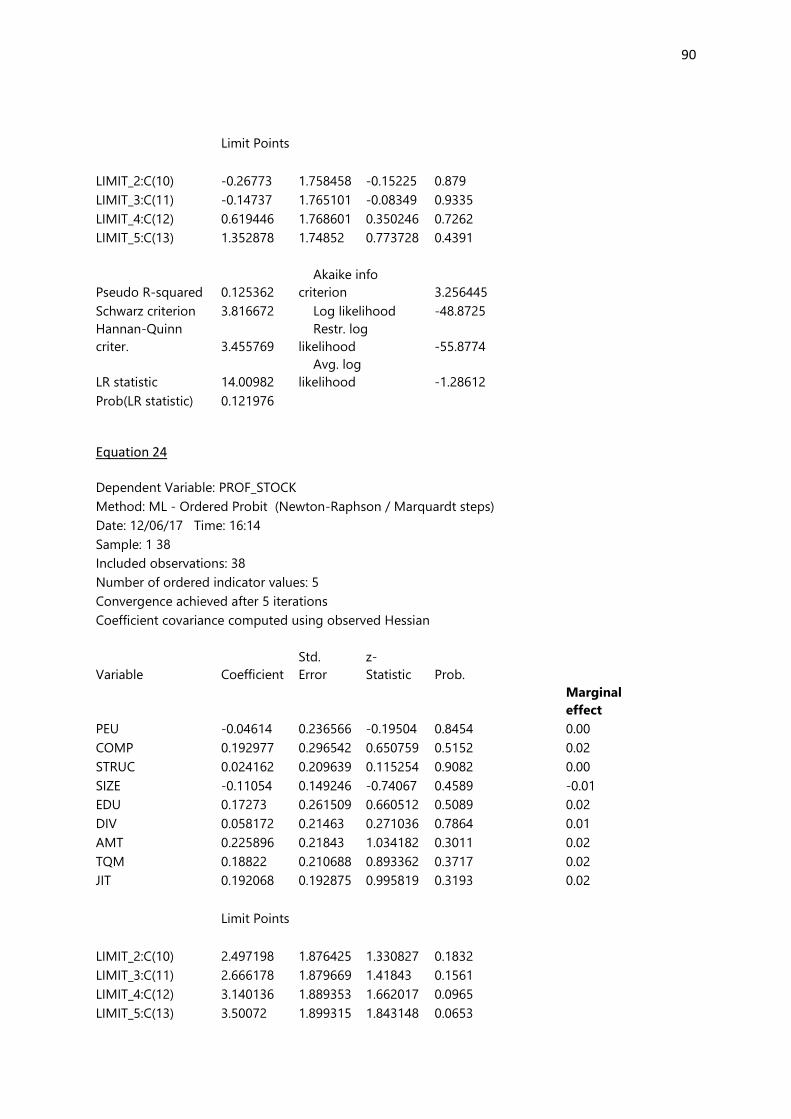
90
Limit Points
LIMIT_2:C(10) -0.26773 1.758458 -0.15225 0.879
LIMIT_3:C(11) -0.14737 1.765101 -0.08349 0.9335
LIMIT_4:C(12) 0.619446 1.768601 0.350246 0.7262
LIMIT_5:C(13) 1.352878 1.74852 0.773728 0.4391
Pseudo R-squared 0.125362
Akaike info
criterion 3.256445
Schwarz criterion 3.816672 Log likelihood -48.8725
Hannan-Quinn
criter. 3.455769
Restr. log
likelihood -55.8774
LR statistic 14.00982
Avg. log
likelihood -1.28612
Prob(LR statistic) 0.121976
Equation 24
Dependent Variable: PROF_STOCK
Method: ML - Ordered Probit (Newton-Raphson / Marquardt steps)
Date: 12/06/17 Time: 16:14
Sample: 1 38
Included observations: 38
Number of ordered indicator values: 5
Convergence achieved after 5 iterations
Coefficient covariance computed using observed Hessian
Variable Coefficient
Std.
Error
z-
Statistic Prob.
Marginal
effect
PEU -0.04614 0.236566 -0.19504 0.8454
0.00
COMP 0.192977 0.296542 0.650759 0.5152
0.02
STRUC 0.024162 0.209639 0.115254 0.9082
0.00
SIZE -0.11054 0.149246 -0.74067 0.4589
-0.01
EDU 0.17273 0.261509 0.660512 0.5089
0.02
DIV 0.058172 0.21463 0.271036 0.7864
0.01
AMT 0.225896 0.21843 1.034182 0.3011
0.02
TQM 0.18822 0.210688 0.893362 0.3717
0.02
JIT 0.192068 0.192875 0.995819 0.3193
0.02
Limit Points
LIMIT_2:C(10) 2.497198 1.876425 1.330827 0.1832
LIMIT_3:C(11) 2.666178 1.879669 1.41843 0.1561
LIMIT_4:C(12) 3.140136 1.889353 1.662017 0.0965
LIMIT_5:C(13) 3.50072 1.899315 1.843148 0.0653
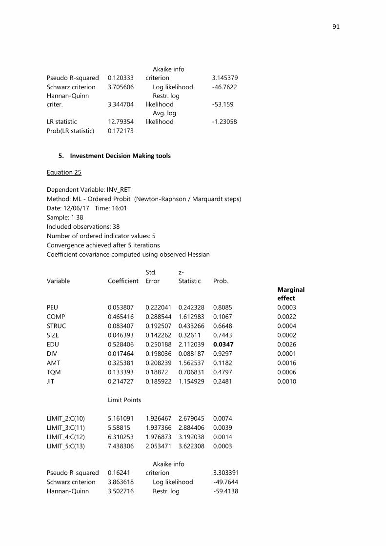
91
Pseudo R-squared 0.120333
Akaike info
criterion 3.145379
Schwarz criterion 3.705606 Log likelihood -46.7622
Hannan-Quinn
criter. 3.344704
Restr. log
likelihood -53.159
LR statistic 12.79354
Avg. log
likelihood -1.23058
Prob(LR statistic) 0.172173
5. Investment Decision Making tools
Equation 25
Dependent Variable: INV_RET
Method: ML - Ordered Probit (Newton-Raphson / Marquardt steps)
Date: 12/06/17 Time: 16:01
Sample: 1 38
Included observations: 38
Number of ordered indicator values: 5
Convergence achieved after 5 iterations
Coefficient covariance computed using observed Hessian
Variable Coefficient
Std.
Error
z-
Statistic Prob.
Marginal
effect
PEU 0.053807 0.222041 0.242328 0.8085
0.0003
COMP 0.465416 0.288544 1.612983 0.1067
0.0022
STRUC 0.083407 0.192507 0.433266 0.6648
0.0004
SIZE 0.046393 0.142262 0.32611 0.7443
0.0002
EDU 0.528406 0.250188 2.112039 0.0347
0.0026
DIV 0.017464 0.198036 0.088187 0.9297
0.0001
AMT 0.325381 0.208239 1.562537 0.1182
0.0016
TQM 0.133393 0.18872 0.706831 0.4797
0.0006
JIT 0.214727 0.185922 1.154929 0.2481
0.0010
Limit Points
LIMIT_2:C(10) 5.161091 1.926467 2.679045 0.0074
LIMIT_3:C(11) 5.58815 1.937366 2.884406 0.0039
LIMIT_4:C(12) 6.310253 1.976873 3.192038 0.0014
LIMIT_5:C(13) 7.438306 2.053471 3.622308 0.0003
Pseudo R-squared 0.16241
Akaike info
criterion 3.303391
Schwarz criterion 3.863618 Log likelihood -49.7644
Hannan-Quinn 3.502716 Restr. log -59.4138
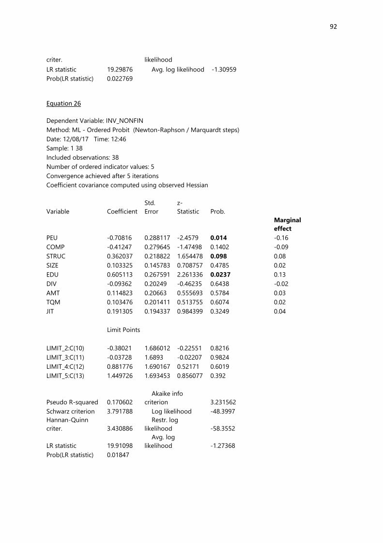
92
criter. likelihood
LR statistic 19.29876 Avg. log likelihood -1.30959
Prob(LR statistic) 0.022769
Equation 26
Dependent Variable: INV_NONFIN
Method: ML - Ordered Probit (Newton-Raphson / Marquardt steps)
Date: 12/08/17 Time: 12:46
Sample: 1 38
Included observations: 38
Number of ordered indicator values: 5
Convergence achieved after 5 iterations
Coefficient covariance computed using observed Hessian
Variable Coefficient
Std.
Error
z-
Statistic Prob.
Marginal
effect
PEU -0.70816 0.288117 -2.4579 0.014
-0.16
COMP -0.41247 0.279645 -1.47498 0.1402
-0.09
STRUC 0.362037 0.218822 1.654478 0.098
0.08
SIZE 0.103325 0.145783 0.708757 0.4785
0.02
EDU 0.605113 0.267591 2.261336 0.0237
0.13
DIV -0.09362 0.20249 -0.46235 0.6438
-0.02
AMT 0.114823 0.20663 0.555693 0.5784
0.03
TQM 0.103476 0.201411 0.513755 0.6074
0.02
JIT 0.191305 0.194337 0.984399 0.3249
0.04
Limit Points
LIMIT_2:C(10) -0.38021 1.686012 -0.22551 0.8216
LIMIT_3:C(11) -0.03728 1.6893 -0.02207 0.9824
LIMIT_4:C(12) 0.881776 1.690167 0.52171 0.6019
LIMIT_5:C(13) 1.449726 1.693453 0.856077 0.392
Pseudo R-squared 0.170602
Akaike info
criterion 3.231562
Schwarz criterion 3.791788 Log likelihood -48.3997
Hannan-Quinn
criter. 3.430886
Restr. log
likelihood -58.3552
LR statistic 19.91098
Avg. log
likelihood -1.27368
Prob(LR statistic) 0.01847
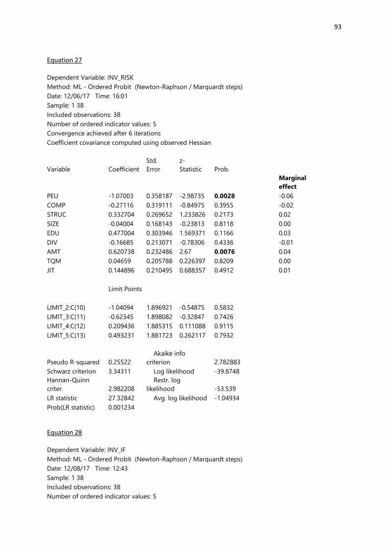
93
Equation 27
Dependent Variable: INV_RISK
Method: ML - Ordered Probit (Newton-Raphson / Marquardt steps)
Date: 12/06/17 Time: 16:01
Sample: 1 38
Included observations: 38
Number of ordered indicator values: 5
Convergence achieved after 6 iterations
Coefficient covariance computed using observed Hessian
Variable Coefficient
Std.
Error
z-
Statistic Prob.
Marginal
effect
PEU -1.07003 0.358187 -2.98735 0.0028
-0.06
COMP -0.27116 0.319111 -0.84975 0.3955
-0.02
STRUC 0.332704 0.269652 1.233826 0.2173
0.02
SIZE -0.04004 0.168143 -0.23813 0.8118
0.00
EDU 0.477004 0.303946 1.569371 0.1166
0.03
DIV -0.16685 0.213071 -0.78306 0.4336
-0.01
AMT 0.620738 0.232486 2.67 0.0076
0.04
TQM 0.04659 0.205788 0.226397 0.8209
0.00
JIT 0.144896 0.210495 0.688357 0.4912
0.01
Limit Points
LIMIT_2:C(10) -1.04094 1.896921 -0.54875 0.5832
LIMIT_3:C(11) -0.62345 1.898082 -0.32847 0.7426
LIMIT_4:C(12) 0.209436 1.885315 0.111088 0.9115
LIMIT_5:C(13) 0.493231 1.881723 0.262117 0.7932
Pseudo R-squared 0.25522
Akaike info
criterion 2.782883
Schwarz criterion 3.34311 Log likelihood -39.8748
Hannan-Quinn
criter. 2.982208
Restr. log
likelihood -53.539
LR statistic 27.32842 Avg. log likelihood -1.04934
Prob(LR statistic) 0.001234
Equation 28
Dependent Variable: INV_IF
Method: ML - Ordered Probit (Newton-Raphson / Marquardt steps)
Date: 12/08/17 Time: 12:43
Sample: 1 38
Included observations: 38
Number of ordered indicator values: 5
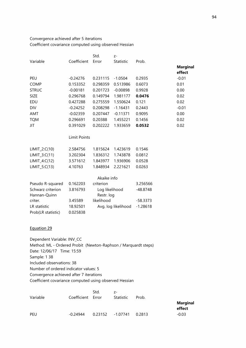
94
Convergence achieved after 5 iterations
Coefficient covariance computed using observed Hessian
Variable Coefficient
Std.
Error
z-
Statistic Prob.
Marginal
effect
PEU -0.24276 0.231115 -1.0504 0.2935
-0.01
COMP 0.153352 0.298359 0.513986 0.6073
0.01
STRUC -0.00181 0.201723 -0.00898 0.9928
0.00
SIZE 0.296768 0.149794 1.981177 0.0476
0.02
EDU 0.427288 0.275559 1.550624 0.121
0.02
DIV -0.24252 0.208298 -1.16431 0.2443
-0.01
AMT -0.02359 0.207447 -0.11371 0.9095
0.00
TQM 0.296691 0.20388 1.455221 0.1456
0.02
JIT 0.391029 0.202222 1.933659 0.0532
0.02
Limit Points
LIMIT_2:C(10) 2.584756 1.815624 1.423619 0.1546
LIMIT_3:C(11) 3.202304 1.836312 1.743878 0.0812
LIMIT_4:C(12) 3.571612 1.843977 1.936906 0.0528
LIMIT_5:C(13) 4.10763 1.848934 2.221621 0.0263
Pseudo R-squared 0.162203
Akaike info
criterion 3.256566
Schwarz criterion 3.816793 Log likelihood -48.8748
Hannan-Quinn
criter. 3.45589
Restr. log
likelihood -58.3373
LR statistic 18.92501 Avg. log likelihood -1.28618
Prob(LR statistic) 0.025838
Equation 29
Dependent Variable: INV_CC
Method: ML - Ordered Probit (Newton-Raphson / Marquardt steps)
Date: 12/06/17 Time: 15:59
Sample: 1 38
Included observations: 38
Number of ordered indicator values: 5
Convergence achieved after 7 iterations
Coefficient covariance computed using observed Hessian
Variable Coefficient
Std.
Error
z-
Statistic Prob.
Marginal
effect
PEU -0.24944 0.23152 -1.07741 0.2813
-0.03
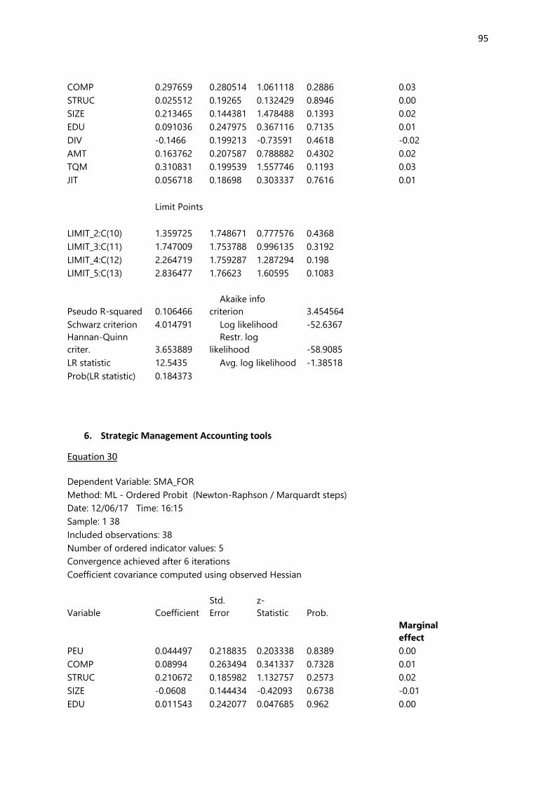
95
COMP 0.297659 0.280514 1.061118 0.2886
0.03
STRUC 0.025512 0.19265 0.132429 0.8946
0.00
SIZE 0.213465 0.144381 1.478488 0.1393
0.02
EDU 0.091036 0.247975 0.367116 0.7135
0.01
DIV -0.1466 0.199213 -0.73591 0.4618
-0.02
AMT 0.163762 0.207587 0.788882 0.4302
0.02
TQM 0.310831 0.199539 1.557746 0.1193
0.03
JIT 0.056718 0.18698 0.303337 0.7616
0.01
Limit Points
LIMIT_2:C(10) 1.359725 1.748671 0.777576 0.4368
LIMIT_3:C(11) 1.747009 1.753788 0.996135 0.3192
LIMIT_4:C(12) 2.264719 1.759287 1.287294 0.198
LIMIT_5:C(13) 2.836477 1.76623 1.60595 0.1083
Pseudo R-squared 0.106466
Akaike info
criterion 3.454564
Schwarz criterion 4.014791 Log likelihood -52.6367
Hannan-Quinn
criter. 3.653889
Restr. log
likelihood -58.9085
LR statistic 12.5435 Avg. log likelihood -1.38518
Prob(LR statistic) 0.184373
6. Strategic Management Accounting tools
Equation 30
Dependent Variable: SMA_FOR
Method: ML - Ordered Probit (Newton-Raphson / Marquardt steps)
Date: 12/06/17 Time: 16:15
Sample: 1 38
Included observations: 38
Number of ordered indicator values: 5
Convergence achieved after 6 iterations
Coefficient covariance computed using observed Hessian
Variable Coefficient
Std.
Error
z-
Statistic Prob.
Marginal
effect
PEU 0.044497 0.218835 0.203338 0.8389
0.00
COMP 0.08994 0.263494 0.341337 0.7328
0.01
STRUC 0.210672 0.185982 1.132757 0.2573
0.02
SIZE -0.0608 0.144434 -0.42093 0.6738
-0.01
EDU 0.011543 0.242077 0.047685 0.962
0.00
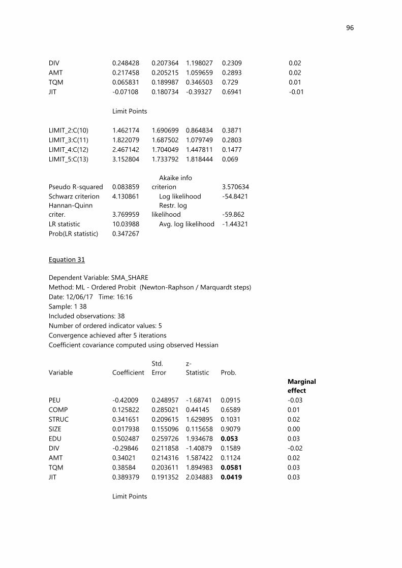
96
DIV 0.248428 0.207364 1.198027 0.2309
0.02
AMT 0.217458 0.205215 1.059659 0.2893
0.02
TQM 0.065831 0.189987 0.346503 0.729
0.01
JIT -0.07108 0.180734 -0.39327 0.6941
-0.01
Limit Points
LIMIT_2:C(10) 1.462174 1.690699 0.864834 0.3871
LIMIT_3:C(11) 1.822079 1.687502 1.079749 0.2803
LIMIT_4:C(12) 2.467142 1.704049 1.447811 0.1477
LIMIT_5:C(13) 3.152804 1.733792 1.818444 0.069
Pseudo R-squared 0.083859
Akaike info
criterion 3.570634
Schwarz criterion 4.130861 Log likelihood -54.8421
Hannan-Quinn
criter. 3.769959
Restr. log
likelihood -59.862
LR statistic 10.03988 Avg. log likelihood -1.44321
Prob(LR statistic) 0.347267
Equation 31
Dependent Variable: SMA_SHARE
Method: ML - Ordered Probit (Newton-Raphson / Marquardt steps)
Date: 12/06/17 Time: 16:16
Sample: 1 38
Included observations: 38
Number of ordered indicator values: 5
Convergence achieved after 5 iterations
Coefficient covariance computed using observed Hessian
Variable Coefficient
Std.
Error
z-
Statistic Prob.
Marginal
effect
PEU -0.42009 0.248957 -1.68741 0.0915
-0.03
COMP 0.125822 0.285021 0.44145 0.6589
0.01
STRUC 0.341651 0.209615 1.629895 0.1031
0.02
SIZE 0.017938 0.155096 0.115658 0.9079
0.00
EDU 0.502487 0.259726 1.934678 0.053
0.03
DIV -0.29846 0.211858 -1.40879 0.1589
-0.02
AMT 0.34021 0.214316 1.587422 0.1124
0.02
TQM 0.38584 0.203611 1.894983 0.0581
0.03
JIT 0.389379 0.191352 2.034883 0.0419
0.03
Limit Points
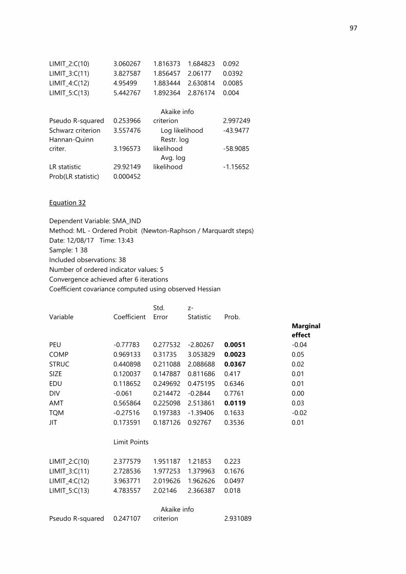
97
LIMIT_2:C(10) 3.060267 1.816373 1.684823 0.092
LIMIT_3:C(11) 3.827587 1.856457 2.06177 0.0392
LIMIT_4:C(12) 4.95499 1.883444 2.630814 0.0085
LIMIT_5:C(13) 5.442767 1.892364 2.876174 0.004
Pseudo R-squared 0.253966
Akaike info
criterion 2.997249
Schwarz criterion 3.557476 Log likelihood -43.9477
Hannan-Quinn
criter. 3.196573
Restr. log
likelihood -58.9085
LR statistic 29.92149
Avg. log
likelihood -1.15652
Prob(LR statistic) 0.000452
Equation 32
Dependent Variable: SMA_IND
Method: ML - Ordered Probit (Newton-Raphson / Marquardt steps)
Date: 12/08/17 Time: 13:43
Sample: 1 38
Included observations: 38
Number of ordered indicator values: 5
Convergence achieved after 6 iterations
Coefficient covariance computed using observed Hessian
Variable Coefficient
Std.
Error
z-
Statistic Prob.
Marginal
effect
PEU -0.77783 0.277532 -2.80267 0.0051
-0.04
COMP 0.969133 0.31735 3.053829 0.0023
0.05
STRUC 0.440898 0.211088 2.088688 0.0367
0.02
SIZE 0.120037 0.147887 0.811686 0.417
0.01
EDU 0.118652 0.249692 0.475195 0.6346
0.01
DIV -0.061 0.214472 -0.2844 0.7761
0.00
AMT 0.565864 0.225098 2.513861 0.0119
0.03
TQM -0.27516 0.197383 -1.39406 0.1633
-0.02
JIT 0.173591 0.187126 0.92767 0.3536
0.01
Limit Points
LIMIT_2:C(10) 2.377579 1.951187 1.21853 0.223
LIMIT_3:C(11) 2.728536 1.977253 1.379963 0.1676
LIMIT_4:C(12) 3.963771 2.019626 1.962626 0.0497
LIMIT_5:C(13) 4.783557 2.02146 2.366387 0.018
Pseudo R-squared 0.247107
Akaike info
criterion 2.931089
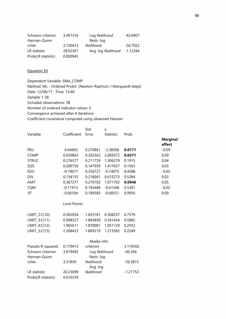
98
Schwarz criterion 3.491316 Log likelihood -42.6907
Hannan-Quinn
criter. 3.130413
Restr. log
likelihood -56.7022
LR statistic 28.02301 Avg. log likelihood -1.12344
Prob(LR statistic) 0.000945
Equation 33
Dependent Variable: SMA_COMP
Method: ML - Ordered Probit (Newton-Raphson / Marquardt steps)
Date: 12/08/17 Time: 13:40
Sample: 1 38
Included observations: 38
Number of ordered indicator values: 5
Convergence achieved after 4 iterations
Coefficient covariance computed using observed Hessian
Variable Coefficient
Std.
Error
z-
Statistic Prob.
Marginal
effect
PEU -0.64602 0.270861 -2.38506 0.0171
-0.09
COMP 0.630863 0.302562 2.085072 0.0371
0.09
STRUC 0.276577 0.211729 1.306279 0.1915
0.04
SIZE 0.209756 0.147959 1.417657 0.1563
0.03
EDU -0.19017 0.256727 -0.74075 0.4588
-0.03
DIV 0.134155 0.218041 0.615273 0.5384
0.02
AMT 0.367277 0.219702 1.671702 0.0946
0.05
TQM -0.11913 0.193484 -0.61568 0.5381
-0.02
JIT -0.00104 0.189383 -0.00551 0.9956
0.00
Limit Points
LIMIT_2:C(10) 0.565054 1.833181 0.308237 0.7579
LIMIT_3:C(11) 0.998327 1.843858 0.541434 0.5882
LIMIT_4:C(12) 1.965611 1.870001 1.051129 0.2932
LIMIT_5:C(13) 2.268453 1.869219 1.213583 0.2249
Pseudo R-squared 0.179412
Akaike info
criterion 3.119265
Schwarz criterion 3.679492 Log likelihood -46.266
Hannan-Quinn
criter. 3.31859
Restr. log
likelihood -56.3815
LR statistic 20.23099
Avg. log
likelihood -1.21753
Prob(LR statistic) 0.016539
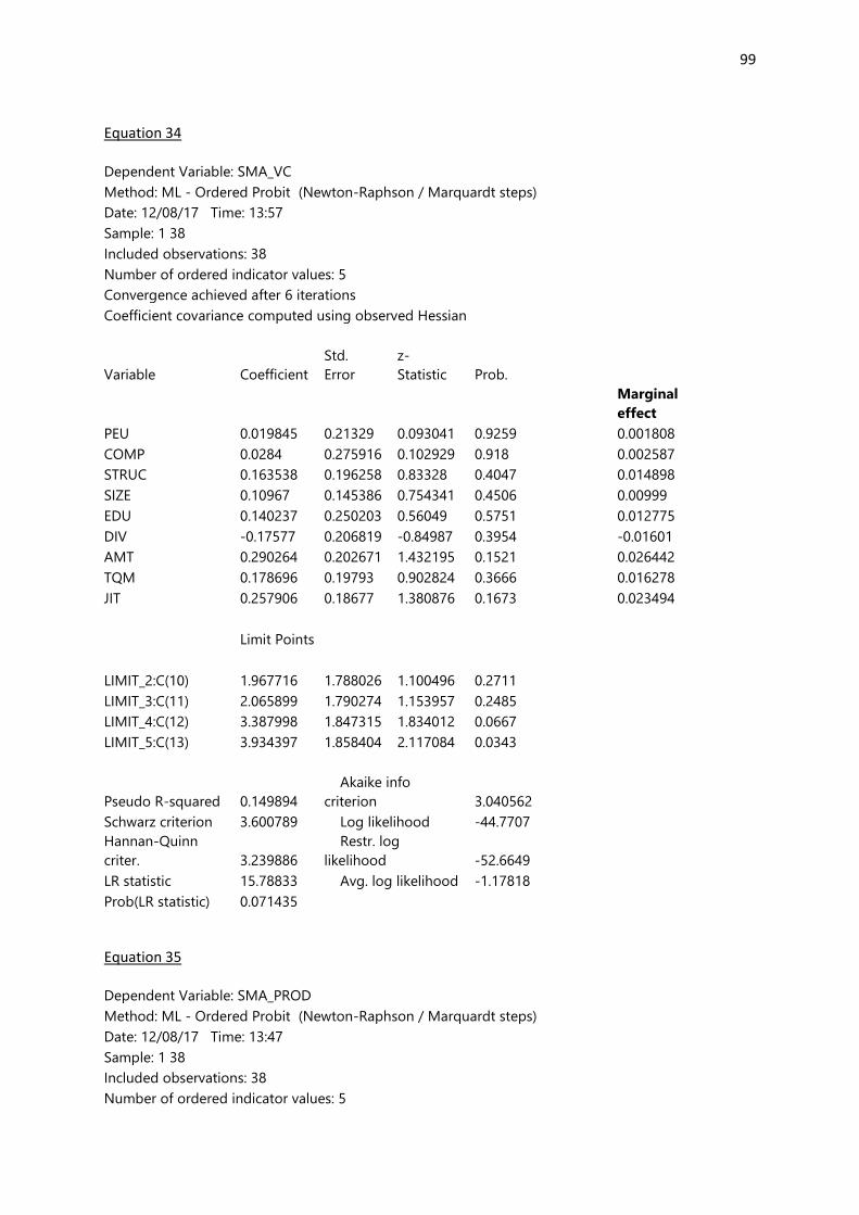
99
Equation 34
Dependent Variable: SMA_VC
Method: ML - Ordered Probit (Newton-Raphson / Marquardt steps)
Date: 12/08/17 Time: 13:57
Sample: 1 38
Included observations: 38
Number of ordered indicator values: 5
Convergence achieved after 6 iterations
Coefficient covariance computed using observed Hessian
Variable Coefficient
Std.
Error
z-
Statistic Prob.
Marginal
effect
PEU 0.019845 0.21329 0.093041 0.9259
0.001808
COMP 0.0284 0.275916 0.102929 0.918
0.002587
STRUC 0.163538 0.196258 0.83328 0.4047
0.014898
SIZE 0.10967 0.145386 0.754341 0.4506
0.00999
EDU 0.140237 0.250203 0.56049 0.5751
0.012775
DIV -0.17577 0.206819 -0.84987 0.3954
-0.01601
AMT 0.290264 0.202671 1.432195 0.1521
0.026442
TQM 0.178696 0.19793 0.902824 0.3666
0.016278
JIT 0.257906 0.18677 1.380876 0.1673
0.023494
Limit Points
LIMIT_2:C(10) 1.967716 1.788026 1.100496 0.2711
LIMIT_3:C(11) 2.065899 1.790274 1.153957 0.2485
LIMIT_4:C(12) 3.387998 1.847315 1.834012 0.0667
LIMIT_5:C(13) 3.934397 1.858404 2.117084 0.0343
Pseudo R-squared 0.149894
Akaike info
criterion 3.040562
Schwarz criterion 3.600789 Log likelihood -44.7707
Hannan-Quinn
criter. 3.239886
Restr. log
likelihood -52.6649
LR statistic 15.78833 Avg. log likelihood -1.17818
Prob(LR statistic) 0.071435
Equation 35
Dependent Variable: SMA_PROD
Method: ML - Ordered Probit (Newton-Raphson / Marquardt steps)
Date: 12/08/17 Time: 13:47
Sample: 1 38
Included observations: 38
Number of ordered indicator values: 5
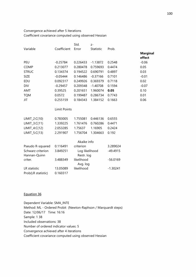
100
Convergence achieved after 5 iterations
Coefficient covariance computed using observed Hessian
Variable Coefficient
Std.
Error
z-
Statistic Prob.
Marginal
effect
PEU -0.25784 0.226433 -1.13872 0.2548
-0.06
COMP 0.213077 0.280478 0.759693 0.4474
0.05
STRUC 0.134374 0.194522 0.690791 0.4897
0.03
SIZE -0.05444 0.146486 -0.37166 0.7101
-0.01
EDU 0.092317 0.249926 0.369379 0.7118
0.02
DIV -0.29457 0.209348 -1.40708 0.1594
-0.07
AMT 0.39525 0.201651 1.960074 0.05
0.10
TQM 0.0572 0.199487 0.286734 0.7743
0.01
JIT 0.255159 0.184343 1.384152 0.1663
0.06
Limit Points
LIMIT_2:C(10) 0.783005 1.755081 0.446136 0.6555
LIMIT_3:C(11) 1.339225 1.761476 0.760286 0.4471
LIMIT_4:C(12) 2.053285 1.75637 1.16905 0.2424
LIMIT_5:C(13) 2.291907 1.756704 1.304663 0.192
Pseudo R-squared 0.116491
Akaike info
criterion 3.289024
Schwarz criterion 3.849251 Log likelihood -49.4915
Hannan-Quinn
criter. 3.488349
Restr. log
likelihood -56.0169
LR statistic 13.05089
Avg. log
likelihood -1.30241
Prob(LR statistic) 0.160317
Equation 36
Dependent Variable: SMA_INTE
Method: ML - Ordered Probit (Newton-Raphson / Marquardt steps)
Date: 12/06/17 Time: 16:16
Sample: 1 38
Included observations: 38
Number of ordered indicator values: 5
Convergence achieved after 4 iterations
Coefficient covariance computed using observed Hessian
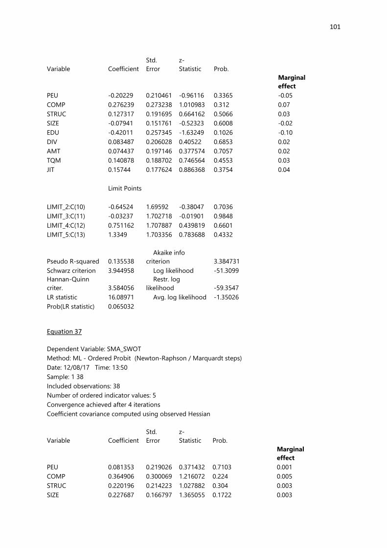
101
Variable Coefficient
Std.
Error
z-
Statistic Prob.
Marginal
effect
PEU -0.20229 0.210461 -0.96116 0.3365
-0.05
COMP 0.276239 0.273238 1.010983 0.312
0.07
STRUC 0.127317 0.191695 0.664162 0.5066
0.03
SIZE -0.07941 0.151761 -0.52323 0.6008
-0.02
EDU -0.42011 0.257345 -1.63249 0.1026
-0.10
DIV 0.083487 0.206028 0.40522 0.6853
0.02
AMT 0.074437 0.197146 0.377574 0.7057
0.02
TQM 0.140878 0.188702 0.746564 0.4553
0.03
JIT 0.15744 0.177624 0.886368 0.3754
0.04
Limit Points
LIMIT_2:C(10) -0.64524 1.69592 -0.38047 0.7036
LIMIT_3:C(11) -0.03237 1.702718 -0.01901 0.9848
LIMIT_4:C(12) 0.751162 1.707887 0.439819 0.6601
LIMIT_5:C(13) 1.3349 1.703356 0.783688 0.4332
Pseudo R-squared 0.135538
Akaike info
criterion 3.384731
Schwarz criterion 3.944958 Log likelihood -51.3099
Hannan-Quinn
criter. 3.584056
Restr. log
likelihood -59.3547
LR statistic 16.08971 Avg. log likelihood -1.35026
Prob(LR statistic) 0.065032
Equation 37
Dependent Variable: SMA_SWOT
Method: ML - Ordered Probit (Newton-Raphson / Marquardt steps)
Date: 12/08/17 Time: 13:50
Sample: 1 38
Included observations: 38
Number of ordered indicator values: 5
Convergence achieved after 4 iterations
Coefficient covariance computed using observed Hessian
Variable Coefficient
Std.
Error
z-
Statistic Prob.
Marginal
effect
PEU 0.081353 0.219026 0.371432 0.7103
0.001
COMP 0.364906 0.300069 1.216072 0.224
0.005
STRUC 0.220196 0.214223 1.027882 0.304
0.003
SIZE 0.227687 0.166797 1.365055 0.1722
0.003
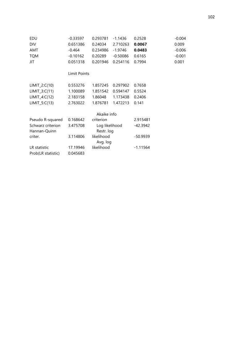
102
EDU -0.33597 0.293781 -1.1436 0.2528
-0.004
DIV 0.651386 0.24034 2.710263 0.0067
0.009
AMT -0.464 0.234986 -1.9746 0.0483
-0.006
TQM -0.10162 0.20289 -0.50086 0.6165
-0.001
JIT 0.051318 0.201946 0.254116 0.7994
0.001
Limit Points
LIMIT_2:C(10) 0.553276 1.857245 0.297902 0.7658
LIMIT_3:C(11) 1.100089 1.851542 0.594147 0.5524
LIMIT_4:C(12) 2.183158 1.86048 1.173438 0.2406
LIMIT_5:C(13) 2.763022 1.876781 1.472213 0.141
Pseudo R-squared 0.168642
Akaike info
criterion 2.915481
Schwarz criterion 3.475708 Log likelihood -42.3942
Hannan-Quinn
criter. 3.114806
Restr. log
likelihood -50.9939
LR statistic 17.19946
Avg. log
likelihood -1.11564
Prob(LR statistic) 0.045683