ON THE ANALYSIS OF OPTICAL MAPPING DATA

by

Deepayan Sarkar

A dissertation submitted in partial fulfillment of

the requirements for the degree of

Doctor of Philosophy

(Statistics)

at the

UNIVERSITY OF WISCONSIN–MADISON

2006

© Copyright by Deepayan Sarkar 2006

All Rights Reserved

i

To my parents.

ii

ACKNOWLEDGMENTS

I would like to thank the many people without whom this work would not have been

possible. The optical mapping system, which forms the basis for this thesis, was pioneered by

Prof David Schwartz and continues to be developed under his leadership at the Laboratory for

Molecular and Computational Genomics at the University of Wisconsin – Madison. Several

people at the lab have helped me understand various aspects of the system: primarily Steve

Goldstein, as well as Rod Runnheim, Chris Churas, Shiguo Zhou and Gus Potamousis. The

optical map data used in this thesis were collected by Alex Lim, Susan Reslewic and Jill

Herschleb. Prof Paul Lizardi’s lab at Yale provided some supplementary data and analysis.

Finally, my advisor Prof Michael Newton provided many important insights throughout the

last few years and helped immensely in shaping the final manuscript.

DISCARD THIS PAGE

iii

TABLE OF CONTENTS

Page

LIST OF TABLES . . . . . . . . . . . . . . . . . . . . . . . . . . . . . . . . . . . . v

LIST OF FIGURES . . . . . . . . . . . . . . . . . . . . . . . . . . . . . . . . . . . vi

ABSTRACT . . . . . . . . . . . . . . . . . . . . . . . . . . . . . . . . . . . . . . . viii

1 Overview of Optical Mapping . . . . . . . . . . . . . . . . . . . . . . . . . . 1

1.1 Background . . . . . . . . . . . . . . . . . . . . . . . . . . . . . . . . . . . . 11.2 Example . . . . . . . . . . . . . . . . . . . . . . . . . . . . . . . . . . . . . . 51.3 Elements of optical mapping . . . . . . . . . . . . . . . . . . . . . . . . . . . 6

1.3.1 Image processing . . . . . . . . . . . . . . . . . . . . . . . . . . . . . 61.3.2 Optical map data . . . . . . . . . . . . . . . . . . . . . . . . . . . . . 101.3.3 Goals and challenges . . . . . . . . . . . . . . . . . . . . . . . . . . . 111.3.4 Algorithms . . . . . . . . . . . . . . . . . . . . . . . . . . . . . . . . 131.3.5 Example (continued) . . . . . . . . . . . . . . . . . . . . . . . . . . . 16

1.4 Outline . . . . . . . . . . . . . . . . . . . . . . . . . . . . . . . . . . . . . . . 20

2 Modeling Optical Map Data . . . . . . . . . . . . . . . . . . . . . . . . . . . 21

2.1 A stochastic model . . . . . . . . . . . . . . . . . . . . . . . . . . . . . . . . 212.1.1 Origin . . . . . . . . . . . . . . . . . . . . . . . . . . . . . . . . . . . 212.1.2 Errors . . . . . . . . . . . . . . . . . . . . . . . . . . . . . . . . . . . 23

2.2 Parameter estimation . . . . . . . . . . . . . . . . . . . . . . . . . . . . . . . 262.2.1 Desorption . . . . . . . . . . . . . . . . . . . . . . . . . . . . . . . . . 272.2.2 Length errors . . . . . . . . . . . . . . . . . . . . . . . . . . . . . . . 312.2.3 Cut errors . . . . . . . . . . . . . . . . . . . . . . . . . . . . . . . . . 31

2.3 Diagnostics . . . . . . . . . . . . . . . . . . . . . . . . . . . . . . . . . . . . 33

3 Significance of Optical Map Alignments . . . . . . . . . . . . . . . . . . . . 37

3.1 Introduction . . . . . . . . . . . . . . . . . . . . . . . . . . . . . . . . . . . . 373.2 Methods . . . . . . . . . . . . . . . . . . . . . . . . . . . . . . . . . . . . . . 39

iv

Page

3.3 Results . . . . . . . . . . . . . . . . . . . . . . . . . . . . . . . . . . . . . . . 403.3.1 Exploration . . . . . . . . . . . . . . . . . . . . . . . . . . . . . . . . 403.3.2 Simplifications . . . . . . . . . . . . . . . . . . . . . . . . . . . . . . . 433.3.3 Simulation . . . . . . . . . . . . . . . . . . . . . . . . . . . . . . . . . 473.3.4 Improving assembly . . . . . . . . . . . . . . . . . . . . . . . . . . . . 47

3.4 Discussion . . . . . . . . . . . . . . . . . . . . . . . . . . . . . . . . . . . . . 493.4.1 Uses . . . . . . . . . . . . . . . . . . . . . . . . . . . . . . . . . . . . 493.4.2 Information measure . . . . . . . . . . . . . . . . . . . . . . . . . . . 513.4.3 Other topics . . . . . . . . . . . . . . . . . . . . . . . . . . . . . . . . 563.4.4 Conclusion . . . . . . . . . . . . . . . . . . . . . . . . . . . . . . . . . 58

4 Detecting Copy Number Polymorphism . . . . . . . . . . . . . . . . . . . . 60

4.1 Introduction . . . . . . . . . . . . . . . . . . . . . . . . . . . . . . . . . . . . 604.2 Methods . . . . . . . . . . . . . . . . . . . . . . . . . . . . . . . . . . . . . . 624.3 Results . . . . . . . . . . . . . . . . . . . . . . . . . . . . . . . . . . . . . . . 674.4 Discussion . . . . . . . . . . . . . . . . . . . . . . . . . . . . . . . . . . . . . 72

5 Future Work . . . . . . . . . . . . . . . . . . . . . . . . . . . . . . . . . . . . . 76

5.1 Alignment . . . . . . . . . . . . . . . . . . . . . . . . . . . . . . . . . . . . . 765.1.1 Score function . . . . . . . . . . . . . . . . . . . . . . . . . . . . . . . 765.1.2 Scale errors . . . . . . . . . . . . . . . . . . . . . . . . . . . . . . . . 77

5.2 Other topics . . . . . . . . . . . . . . . . . . . . . . . . . . . . . . . . . . . . 80

LIST OF REFERENCES . . . . . . . . . . . . . . . . . . . . . . . . . . . . . . . 82

APPENDICES

Appendix A: Score functions for alignment . . . . . . . . . . . . . . . . . . . . . 85Appendix B: Hidden Markov Model calculations . . . . . . . . . . . . . . . . . . 87

DISCARD THIS PAGE

v

LIST OF TABLES

Table Page

1.1 Summary of two optical map data sets . . . . . . . . . . . . . . . . . . . . . . . 5

1.2 Summary of variations detected in CHM and GM07535 . . . . . . . . . . . . . 19

3.1 Percentage of GM07535 maps declared significant . . . . . . . . . . . . . . . . . 46

3.2 Percentage of GM07535 maps declared significant by the SOMA and LR scores . 50

4.1 AIC and BIC values for HMM fits . . . . . . . . . . . . . . . . . . . . . . . . . 70

DISCARD THIS PAGE

vi

LIST OF FIGURES

Figure Page

1.1 Diagrammatic overview of optical mapping . . . . . . . . . . . . . . . . . . . . 4

1.2 Close-up of optical map image . . . . . . . . . . . . . . . . . . . . . . . . . . . 7

1.3 Intensity profiles . . . . . . . . . . . . . . . . . . . . . . . . . . . . . . . . . . . 7

1.4 Estimation of scale across channel surface . . . . . . . . . . . . . . . . . . . . . 9

1.5 Visualization of optical map alignments . . . . . . . . . . . . . . . . . . . . . . 17

1.6 Visualization of optical map assembly . . . . . . . . . . . . . . . . . . . . . . . 18

2.1 Distribution of restriction fragment lengths . . . . . . . . . . . . . . . . . . . . 22

2.2 Quantile plot illustrating desorption . . . . . . . . . . . . . . . . . . . . . . . . 29

2.3 Non-parametric Grenander estimator of desorption rate . . . . . . . . . . . . . 30

2.4 Variance models for observed fragments sizes . . . . . . . . . . . . . . . . . . . 32

2.5 Distribution of fragment length errors . . . . . . . . . . . . . . . . . . . . . . . 32

2.6 Diagnostic plot: quantiles of fragment lengths . . . . . . . . . . . . . . . . . . . 34

2.7 Diagnostic plot: mean difference plot . . . . . . . . . . . . . . . . . . . . . . . . 35

2.8 Diagnostic plot: hanging rootogram for number of fragments . . . . . . . . . . . 36

3.1 Independence of in silico fragment lengths . . . . . . . . . . . . . . . . . . . . . 41

3.2 Dependence of spurious scores on optical map . . . . . . . . . . . . . . . . . . . 42

3.3 Null distribution of difference between optimal scores . . . . . . . . . . . . . . . 44

3.4 Variance of errors . . . . . . . . . . . . . . . . . . . . . . . . . . . . . . . . . . 44

vii

Figure Page

3.5 Parametric models for µ(M) . . . . . . . . . . . . . . . . . . . . . . . . . . . . . 45

3.6 Comparison of significance strategies using iterative assembly . . . . . . . . . . 48

3.7 LR scores for ungapped global alignment . . . . . . . . . . . . . . . . . . . . . . 50

3.8 Optimal scores vs self-alignment score . . . . . . . . . . . . . . . . . . . . . . . 52

3.9 Self-score plot for simulated data . . . . . . . . . . . . . . . . . . . . . . . . . . 54

3.10 Thinning of coverage in optical map alignments . . . . . . . . . . . . . . . . . . 55

3.11 Estimated thinning rates . . . . . . . . . . . . . . . . . . . . . . . . . . . . . . 56

3.12 Effect of permutations on test statistics . . . . . . . . . . . . . . . . . . . . . . 59

4.1 Power function . . . . . . . . . . . . . . . . . . . . . . . . . . . . . . . . . . . . 64

4.2 Results of one simulation run . . . . . . . . . . . . . . . . . . . . . . . . . . . . 68

4.3 Summary of several simulation runs . . . . . . . . . . . . . . . . . . . . . . . . 69

4.4 The GM07535 genome compared to CHM . . . . . . . . . . . . . . . . . . . . . 71

4.5 Results for MCF-7 chromosomes 17 and 20 . . . . . . . . . . . . . . . . . . . . 73

5.1 Correlation of sizing errors within map . . . . . . . . . . . . . . . . . . . . . . . 78

5.2 Improvement in optimal alignment score . . . . . . . . . . . . . . . . . . . . . . 79

ON THE ANALYSIS OF OPTICAL MAPPING DATA

Deepayan Sarkar

Under the supervision of Professor Michael A. Newton

At the University of Wisconsin-Madison

Whole genome analysis of variation is becoming possible with improved biotechnology,

and this is anticipated to have profound implications for biology and medicine. Ideally,

one would like to record a sampled genome at the nucleotide level, but this goal remains

beyond our reach in spite of the fact that we now have a finished reference copy for several

species. Using well-defined genomic markers, physical maps represent a genome at a lower

resolution than nucleotide sequence. In particular, optical mapping produces physical maps

based on coordinates of recognition sites of specific restriction enzymes. Optical mapping is

well developed for small (e.g. microbial) genomes, and recent advances have enabled optical

mapping of mammalian-sized genomes as well. This development, however, raises important

new computational and statistical questions. The availability of reference genomes has been

instrumental in the development of methods based on optical mapping to detect within-

species variation, by serving as the basis for comparison with a sampled genome. Reference

copies also open up other, less obvious, possibilities that impact the understanding and

statistical analysis of optical mapping data. In this thesis we explore some such possibilities,

particularly in the context of large genomes. In particular, we address parameter estimation

in optical map models, the assessment of significance of optical map alignments, and the use

of optical map data to detect copy number alterations.

Michael A. Newton

viii

ABSTRACT

Whole genome analysis of variation is becoming possible with improved biotechnology,

and this is anticipated to have profound implications for biology and medicine. Ideally,

one would like to record a sampled genome at the nucleotide level, but this goal remains

beyond our reach in spite of the fact that we now have a finished reference copy for several

species. Using well-defined genomic markers, physical maps represent a genome at a lower

resolution than nucleotide sequence. In particular, optical mapping produces physical maps

based on coordinates of recognition sites of specific restriction enzymes. Optical mapping is

well developed for small (e.g. microbial) genomes, and recent advances have enabled optical

mapping of mammalian-sized genomes as well. This development, however, raises important

new computational and statistical questions. The availability of reference genomes has been

instrumental in the development of methods based on optical mapping to detect within-

species variation, by serving as the basis for comparison with a sampled genome. Reference

copies also open up other, less obvious, possibilities that impact the understanding and

statistical analysis of optical mapping data. In this thesis we explore some such possibilities,

particularly in the context of large genomes. In particular, we address parameter estimation

in optical map models, the assessment of significance of optical map alignments, and the use

of optical map data to detect copy number alterations.

1

Chapter 1

Overview of Optical Mapping

1.1 Background

Completion of the Human Genome Project (International Human Genome Sequencing

Consortium, 2004, Build 35) stands as a critical landmark in science and medicine. All kinds

of biological mysteries may be unlocked with keys buried in the full genomic sequence. Of

course, the particular sequence documented online is a single reference copy. Its structure

and basic content are shared by all humans, but plasticity and variation in the genome

underlie both normal biology and disease. Such variations include insertions, deletions, rear-

rangements, single nucleotide polymorphisms (SNPs) and copy number changes. Measuring

how much and in what manner one human genome varies from another is a central problem

of the genomic sciences. A direct approach to detect all the differences between two genomes

would be to sequence each genome separately, but this is not feasible with current technol-

ogy. Sequencing costs are high and the effort required to construct even a single genome

is considerable. In any case, differences are likely to represent only a tiny fraction of the

genome. Research on various alternative methods to study genome-wide structural variation

is ongoing, some of which are summarized by Eichler (2006).

Physical maps: Information about genomic variation can also be obtained from lower

resolution representations of the genome that do not record the full nucleotide sequence, such

as physical maps. A physical map is a listing of the locations along the genome where certain

markers occur. Typically, each marker is a short, well defined nucleotide sequence, such as

2

the recognition sequence of a restriction enzyme (more below). The ordered sequence of

distances in base pairs between successive marker positions summarizes the genome sequence

and can be viewed as a sort of bar code of the genome. Genomic differences can affect the

presence or absence of markers, the distances between them and their orientation, inducing

analogous changes in the bar code. Thus, by comparing physical maps instead of the full

nucleotide sequences, we can detect an important subset of structural genomic variation,

especially indels and translocations that are difficult to detect with many other technologies.

In this thesis we consider statistics for Optical Mapping, a system to study a particular class

of physical maps known as restriction maps.

Restriction maps: A restriction map is a physical map induced by restriction enzymes.

These DNA scissors, as they have been called, occur naturally in bacteria, where they act as

a defense mechanism by cutting up foreign (usually virus) DNA molecules at any occurrence

of a certain recognition sequence. Sites on the molecule where this sequence occurs are

known as restriction sites or recognition sites and stretches of DNA between successive sites

are called restriction fragments. For instance, the enzyme SwaI, denoted 5′-ATTT|AAAT-

3′, recognizes the sequence ATTTAAAT, cutting between the 4th and 5th nucleotides. This

restriction site appears more than 225000 times in Build 35 of the human genome, with more

or less random fragment sizes (see Figures 2.1 and 3.1). Different enzymes have different

recognition sequences and thus provide different physical maps. Note that having a reference

copy of the human genome allows us to perform such in silico 1 experiments. The availability

of in silico reference maps can be extremely helpful, and their use is a recurrent theme in

this thesis.

In early experiments with restriction maps, the problem was to reconstruct the underlying

map from data on only the sizes of restriction fragments, without direct information on their

ordering (Waterman, 1995; Setubal and Meidanis, 1997). Examples of such experiments

include the double digest and partial digest problems. These problems are computationally

1in the computer

3

hard, do not always have a unique solution, and may not scale well. Additionally, these

methods typically require measurements from multiple copies of the target DNA, usually

through the creation of clone libraries.

Optical mapping: Optical mapping (Schwartz et al., 1993; Dimalanta et al., 2004) pro-

duces ordered restriction maps from single DNA molecules. Briefly, DNA from hundreds of

thousands of cells in solution is randomly sheared to produce pieces that are around 500 Kb

long. The solution is then passed through a micro-channel, where the DNA molecules are

stretched and then attached to a positively charged glass support. A restriction enzyme is

then applied, cleaving the DNA at corresponding restriction sites. The DNA molecules re-

main attached to the surface, but the elasticity of the stretched DNA pulls back the molecule

ends at the cleaved sites. The surface is photographed under a microscope after being stained

with a fluorochrome. The cleavage sites show up in the image as tiny gaps in the fluores-

cent line of the molecule, giving an snapshot of the full restriction map. Even though these

molecules are large by many standards, they may still represent only a small fraction of the

chromosome they come from. Naturally, the amount of information in an optical map data

set is related to the size of the underlying genome. It is common to measure the effective

size of a data set by its coverage, which is the ratio of the accumulated lengths of all optical

maps and the estimated length of the genome.

Several types of noise affect optical map data, and a reliable picture of the true map can

only be obtained by combining information from multiple optical maps that redundantly tile

the genome. Most of the algorithmic challenges in optical mapping stem from trying to model

the various kinds of noise, which are not all completely understood, and making inferences

about the underlying map. Figure 1.1 outlines the basic steps of data collection, image

processing and data analysis that together form the cornerstones of the optical mapping

system.

Uses: Optical mapping has various applications. It has been successfully used to assist in

sequence assembly and validation efforts (Ivens et al., 2005; Armbrust et al., 2004), usually

4

Figure 1.1 Diagrammatic overview of optical mapping. DNA from many thousands of cells,each representing a copy of the genome being studied, is passed through microfluidic channels(a.k.a. groups) where they are stretched and attached to a positively charged glass surface.After a restriction enzyme is applied, the surface is imaged using fluorescence microscopy.DNA molecules appear as bright fluorescent pixels, which are subsequently identified andconverted into candidate restriction maps in the image processing step. Statistical analysisis concerned largely with calculations post image processing, although it does inform theprevious steps as well.

5

for microbial and other small genomes. In the early stages of a sequencing project, a genome-

wide restriction map provides ordering and orientation information for sequence contigs. In

later stages, optical mapping can be used to validate ordering and orientation, estimate

sequence gap sizes, and identify potential misassemblies. Recently, the focus of optical

mapping has changed in two important ways. First, the ability to automate image processing

and much of the subsequent analysis has made it practical to collect and analyze very large

data sets. This allows the study of large genomes. Second, as more and more high quality

sequence information has become available, the detection of genomic variation has emerged

as a major goal of optical mapping. The construction of restriction maps to aid sequencing is

still important for organisms where sequence information is absent or incomplete. This is a

particularly challenging task for large genomes, with mixed success so far. In this thesis, we

will largely restrict our attention to the case where a high quality reference copy is available.

1.2 Example

Throughout the thesis, we use optical map data recently collected and reported by

Reslewic et al. (unpublished) to illustrate specific ideas. The data were obtained from two hu-

man cell sources. One was a normal diploid male lymphoblastoid cell line GM07535 (Coriell

Cell Repositories, Camden, NJ). The other was a complete hydatidiform mole (CHM), arti-

ficially created to be homozygous (Fan et al., 2002). The restriction enzyme SwaI was used

in both cases. Table 1.1 gives some basic numerical summaries of the two data sets.

Source CHM GM07535

Number of maps 416284 206796

Avg. molecule size (Kb) 436.5 441.9

Avg. fragment size (Kb) 21.3 20.2

Total map mass (Mb) 187386 91915

Approximate coverage 62.1 29.9

Table 1.1 Summary of the CHM and GM07535 data sets

6

1.3 Elements of optical mapping

We now describe in more depth elements of a typical optical mapping experiment. We

start with image processing and go on to discuss the structure of optical map data and

the goals and challenges we face in data analysis. We describe two basic computational

tasks, alignment and assembly, that are fundamental in addressing many other problems.

We end with a summary of the analysis of the GM07535 and CHM data sets reported by

Reslewic et al..

1.3.1 Image processing

Intensity profiles: For a typical optical mapping experiment, hundreds of raw images

need to be processed to obtain useful data (Figure 1.2). The first step in this process is to

identify the collections of pixels in an image that together represent a single DNA molecule.

This is a complicated task that falls in the domain of computer vision and will not be

discussed further. The end product of this step is an intensity profile for each molecule

(Figure 1.3) giving the measured fluorescent intensity as a function of distance along the

“backbone”. There are two ways to proceed. We may consider these profiles as our primary

data, and retain the information they contain in subsequent analyses. Alternatively, we may

immediately convert them into putative restriction maps, i.e. to an ordered sequence of

fragment lengths. The second approach is simpler because it separates the problem into two

parts that can be refined independently. Also, many standard techniques in computational

biology apply, with suitable adaptations, in this formulation. The first approach has a certain

appeal, but presents difficult challenges and we do not investigate it further. The rest of this

discussion assumes the second, two-step approach.

Cleavage sites: To convert intensity profiles to restriction maps, one has to first identify

the cleavage sites or cut sites in the map, indicated by ‘dips’ in the intensity profile. The

approaches traditionally used to identify cut sites are largely heuristic, although formal

7

Figure 1.2 Close-up of a typical optical map image with (bottom) and without (top) opticalmaps marked up. The colors are reversed for legibility, so DNA molecules are representedby dark pixels against a light background. The image processing step is complex, and issummarized only briefly in the text.

Figure 1.3 Examples of intensity profiles from 5 different molecules. Cuts are indicated bydips in the intensity.

8

statistical techniques may also be used. Naturally, not all cuts present are always detected,

nor are all reported cuts real.

Lengths: Once cut sites are identified, the intensity profile between cuts is integrated to

obtain a total intensity of the corresponding restriction fragment. These measurements then

need to be scaled appropriately to convert them to base pair units. Due to variability in

experimental conditions, the scale factor is usually different in different surfaces and channels,

and possibly even within a channel. To deal with this, DNA molecules with known length

and restriction pattern, called standards, are placed in the sample along with the DNA

being mapped. These standards are identified in the images based only on their pattern.

Their measured fluorescent lengths and known base-pair lengths are then used to scale other

fragments. Naturally, the measured intensities of the standards are themselves subject to

noise, and the scale is usually estimated as a smooth function of position on the image.

Figure 1.4 shows the distribution of standards on a typical surface along with the estimated

scale.

Quality: A critical theme in the optical mapping system is the automated processing of

massive amounts of data, beginning with image processing. Only a fraction of the fluorescent

material seen in raw images is ever marked up by the image processing step and reported as

optical maps. This filtering is important to ensure a certain minimal quality in the optical

map data one works with. Of course, the automated processing is not perfect and certain

maps are marked up wrongly; subsequent methods need to be able to deal robustly with

these errors. Most existing methods treat all maps equally once they are reported by the

image processing software. However, it is likely that some weight or measure of confidence

reported along with every map would be useful in further analysis. This is an area that could

benefit from further research.

9

Offset along channel (pixels)

Offs

et a

cros

s ch

anne

l (pi

xels

)

−400

−200

0

200

20000 40000 60000 80000 100000

0.96 0.98 1.00 1.02 1.04

Figure 1.4 Estimated scale factor (relative to mean) across the surface of a typical channel,showing spatial dependence. The estimated scale here is based on a LOESS smooth ofmeasured intensities of ‘standards’, which are housekeeping molecules of known genomiclength and restriction pattern. The locations of these standards, identified by their pattern,are indicated by white dots on the figure above. Black dots represent locations of identifiedoptical map fragments.

10

1.3.2 Optical map data

Representation: An optical map identified by image processing is essentially an ordered

sequence of fragment lengths. Thus, an optical map with n fragments may be denoted as

x = (x1, . . . , xn)

where xi is the measured length of the ith fragment. Another natural representation of an

optical map is as a sequence of recognition sites. An optical map x is easily converted into a

sequence of cut sites by accumulating the lengths, noting that the cut sites are only defined

up to location. Denoting the conversion from fragment lengths to cut site locations by S,

we may write

S(x) ={

0 = s0 < s1 < · · · < sn =∑

xi

}

where xi = si−si−1 for i = 1, . . . , n are fragment lengths and si =∑i

j=0 xj are locations of cut

sites. The endpoints s0 and sn are not treated as cut site locations since they represent breaks

that define the original molecule as a segment of the whole genome (from shearing) rather

than breaks created by the restriction enzyme. The first representation, being invariant to

origin, has the advantage of being unambiguous, but the second is often more useful, e.g.

for defining alignments between two or more optical maps. Of course, both representations

apply to any physical map. Optical maps may have additional meta-data associated with

them (e.g. confidence scores from image processing), but most existing algorithms ignore

such attributes.

Characteristics: Optical map molecules are generally regarded as random snapshots ob-

tained from the underlying genome, i.e., their locations are assumed to be uniformly dis-

tributed within the genome. Their orientation is not known a priori. The lengths of the

molecules vary; a typical molecule may be around 500 Kb long, and 1000 Kb molecules are

not uncommon. Unlike sequence reads that are obtained as averages over many copies of a

clone, optical maps represent single molecules derived from genomic DNA, providing a more

11

direct glimpse at the underlying structure of the genome. Unfortunately, this also means

that raw optical maps can be fairly noisy. In particular,

• not all true restriction sites are observed, i.e. some cuts are missing, due to imperfect

digestion by the restriction enzyme

• breakage of DNA may cause spurious cuts to appear in a map

• measurement of fluorescent intensities and conversion to base pairs is inaccurate, caus-

ing sizing errors in fragment lengths

• relatively small fragments (say 5 Kb or less) may lose adhesion to the surface and des-

orb, in which case they are not included in the final map. Some of these fragments may

re-attach themselves near other fragments, potentially causing length overestimation

in the latter.

All these noises are confounded with image processing errors. Mistakes in image processing

may also cause optical chimeras, where unrelated maps are marked up as one because they

overlap on the image. Other less systematic errors are also present. These errors, along

with the choice of restriction enzyme and genome, affect the typical size of an optical map

fragment. The average fragment size, often used to summarize an optical map data set, is

usually between 5 and 40 Kb.

1.3.3 Goals and challenges

Goals: A typical optical mapping experiment begins with the collection of data followed by

image processing to identify individual optical maps. The goal of subsequent analysis depends

partly on the genome being mapped. Although the goal of optical mapping is always to make

inferences about the underlying restriction map, it is important to distinguish between cases

where a draft reference sequence of the organism is available and ones where it is not. In the

latter case, the goal of optical mapping is de novo assembly, i.e. to reconstruct the underlying

restriction map, often to assist in sequencing efforts. In the former case, a possible candidate

12

restriction map can be derived in silico by identifying the enzyme recognition pattern in

the reference sequence, and the primary goal of optical mapping is to determine how the

genome under study differs from the reference copy in terms of their respective restriction

maps. Such differences can be due to errors in the sequence, especially in the early stages

of sequencing, but more importantly, they can reflect real biological variation. In either

case, these broad goals are often tackled by breaking them down into smaller, more tractable

problems.

Algorithmic challenges: Optical mapping has been very successful in obtaining restric-

tion maps of relatively small genomes (e.g. microbes). A critical component of this success

has been algorithmic research in the 1990’s specifically aimed at optical mapping data, no-

tably the work of Anantharaman et al. (1999) leading to the Gentig assembly software. With

recent technological advances, the focus has shifted to larger genomes. The primary challenge

introduced by this shift is scalability. Computational methods that work well for microbial

genomes may fail for large genomes due to memory and speed limits of existing computational

systems. Since mammalian genomes differ in size from microbial genomes by several orders

of magnitude, the relative coverage may be far less. Careful statistical analysis is thus critical

in making full use of the available data. New methods are also required to take advantage of

in silico maps when they are available. It should be noted that restriction maps have many

fundamental similarities with sequence data, and algorithms developed for sequence analysis

can often be adapted to work with optical maps (e.g. Huang and Waterman, 1992).

Validation: Due to the nature of optical mapping data, it is rarely possible to know the

true answer except in very special circumstances. It is therefore natural to use simulation to

validate algorithmic techniques. While this has been implicitly acknowledged in much of the

algorithmic work on optical mapping, we think that the stochastic model used in simulation

itself deserves closer attention. With the large data sets that are now available, we can also

hope to use the data to validate models, at least in some limited ways. In particular, we

have found graphical diagnostics to be particularly useful in model checking (see Section 2.3),

13

which is not surprising since well designed graphs can usually convey complex information

more effectively than numerical summaries.

1.3.4 Algorithms

Problems in optical mapping are often approached indirectly by trying to answer simpler,

more specific ones. This is not uncommon in computational biology, where the complexity

of a problem may make a holistic solution difficult. Two algorithmic questions that play a

recurrent role in many of these approaches are alignment and assembly. Each tries to answer

a particular problem; however, it is often more useful to think of these as tools rather than

solutions. Here, we give an overview of these two fundamental computational tasks.

Alignment

The problem of alignment is to detect association or overlap between two or more re-

striction maps. Such association is measured by a score function which assigns a numerical

measure of goodness to any potential alignment. Of course different score functions may

be used and much rests on choosing a suitable score function. Waterman et al. (1984) pre-

sented a score function for restriction map comparison, which was subsequently extended by

Huang and Waterman (1992). Valouev et al. (2006) have developed scores functions for the

comparison problem specifically in the context of optical mapping. These score functions

have been derived as model-based likelihood ratio test statistics, although this is not strictly

necessary (Appendix A).

Given a suitable score function, dynamic programming is used to efficiently search for

optimal alignments. In the context of alignment against a reference, for example, every indi-

vidual optical map must be scored across the genome. Alignment algorithms for nucleotide

sequence data, such as the Needleman-Wunsch and Smith-Waterman algorithms, can be

adapted to work with restriction maps. Certain modifications are required to enable such

use; these are described by Valouev et al. (2006).

14

Significance: An optimal alignment exists in any map comparison problem, irrespective

of any actual association. In order to minimize the potential effects of misaligned maps, it is

essential to limit alignments by some additional criterion. This is the problem of assessing

the significance of a given alignment. The significance problem in optical map alignment

is more difficult than in sequence alignment, because of a greater degree of noise and also

because of differences in the nature of the data. We find deficiencies in the current state of

the art, and in Chapter 3 we introduce and evaluate an alternative approach to measuring

the significance of optical map alignments. Here, we give a general overview of the mechanics

of map alignment.

Notation: We restrict our attention to pairwise alignments, i.e. those between two re-

striction maps. Let x = (x1, . . . , xm) and y = (y1, . . . , yn) denote two restriction maps with

m and n fragments respectively. Let the corresponding representations in terms of cut sites

be S(x) = {s0 < s1 < · · · < sm} and S(y) = {t0 < t1 < · · · < tn}. An alignment between x

and y can be represented by an ordered set of index pairs

C =((

i1j1

),(i2j2

), . . . ,

(ikjk

))

indicating a correspondence between the cut sites siℓ and tjℓ for ℓ = 1, . . . , k, where 0 < i1 <

· · · < ik < m and 0 < j1 < · · · < jk < n. To allow missing fragments in the alignment, this

last condition can be modified to allow successive indices to be equal, as long as successive

index pairs are not identical. For non-trivial alignments k ≥ 2, in which case the alignment

consists of k−1 aligned chunks. The ℓth chunk (ℓ = 1, . . . , k−1) has lengths xℓ = siℓ −siℓ−1,

and yℓ = tjℓ − tjℓ−1involving mℓ = iℓ − iℓ−1 and nℓ = jℓ − jℓ−1 fragments respectively in

the original maps x and y. To be used successfully in a dynamic programming algorithm, a

score function must be additive, in the sense that the score of a complete alignment must be

the sum of the scores for its component chunks.

15

Gapped alignments: The above description implicitly assumes that given any two cut

sites involved in the alignment, all intermediate cut sites will also be involved. Such align-

ments are known as ungapped alignments. One may wish to relax this assumption and allow

gaps, e.g. to represent deletions or insertions. The above notation can be easily generalized

to include such gapped alignments by allowing some index pairs to attain a special value

representing a boundary, e.g.(iℓjℓ

)=

(NANA

). In principle the requirement that iℓ’s and jℓ’s

be increasing can also be relaxed to allow change in orientation within an alignment (e.g. to

represent inversion) but this is rarely allowed in practice due to difficulty in implementation.

The true orientation of raw optical maps are unknown, so both must be considered during

analysis.

Map types: x and y above denote generic restriction maps. In practice, they can be one

of three types; individual optical maps, reference maps derived in silico from sequence and

intermediate consensus maps derived by combining multiple optical maps. This distinction is

important when comparing two maps. For example, optical maps are noisy whereas in silico

reference maps are generally considered error free. Consensus maps lie somewhere in between,

since they contain information averaged over individual optical maps. Thus, comparing an

optical map with another optical map is a symmetric problem, whereas comparing an optical

map with an in silico reference or a consensus map is not.

Alignment types: Most types of sequence alignment problems have a corresponding map

alignment problem. Terminology regarding the various types of alignment are not standard,

so we refrain from giving a full list and refer the reader to their favorite book on sequence

alignment, e.g. Waterman (1995). Two variants of global alignment have been particularly

useful in recent work: overlap alignment, where a suffix of one map is aligned to a prefix of

another, and fit alignment, where an alignment is desired for a map so that it is completely

contained in another, usually much larger, map. Local alignments are another important

class of alignments that are potentially useful in identifying structural variation, but have

not been studied extensively in this context.

16

Software: The SOMA software suite can be used to perform restriction map alignments.

As in sequence alignment, one is often interested in sub-optimal alignments as well, i.e. high-

scoring alignments in addition to the top-scoring one. SOMA is able to find such alignments.

Genspect can be used to visualize alignments reported by SOMA. Figure 1.5 shows a typical

visualization of optical map alignments.

Assembly

The assembly problem can be viewed as a multiple alignment problem, with an additional

step of producing an inferred consensus map. The most successful optical map assembly soft-

ware to date is Gentig, based on ideas described in Anantharaman et al. (1997) (for clones)

and Anantharaman et al. (1999) (for genomic DNA). Briefly, they develop a Bayesian ap-

proach where a prior model for the unknown restriction map and a conditional distribution

for optical maps given the true map are used to derive the posterior density for an hypothe-

sized map. The inferred restriction map is, in principle, the one that maximizes this posterior

density. Due to the complexities of the problem, a complete search is infeasible, and various

heuristics are employed to enable an efficient implementation. We have little to add on the

assembly problem, and refer the reader to the original papers for further details. Gentig

results can also be visualized using Genspect, as shown in Figure 1.6.

1.3.5 Example (continued)

The goal of an optical mapping project is to infer the underlying restriction map of the

genome being studied. For small genomes, Gentig serves this purpose well. However, for

large genomes such as GM07535 and CHM (Table 1.1), the sizes of the data sets exceeds its

capacity, and new algorithms are required. Fortunately, additional information is available

for these data sets in the form of an in silico reference map, derived from the human genome

sequence by locating instances of the SwaI recognition pattern. The genomes being studied

are largely similar to this reference, so we are primarily interested in how their restriction

maps differ from the reference.

17

Figure 1.5 A visualization of alignments of optical maps to an in silico reference. Thealignments were done using SOMA, and Genspect was used to visualize the results. Thetop row represents a segment of the in silico map derived from the human genome, towhich optical maps were aligned. The optical map fragments are color coded to indicate cutdifferences and jittered vertically to emphasize fragment boundaries.

18

Figure 1.6 A visualization, using Genspect, of an assembled consensus map, along withoptical maps that support it. The assembly was produced by Gentig. The visualization issimilar to that in Figure 1.5, with the exception that the top row represents the assembledconsensus map rather than the predefined alignment target.

19

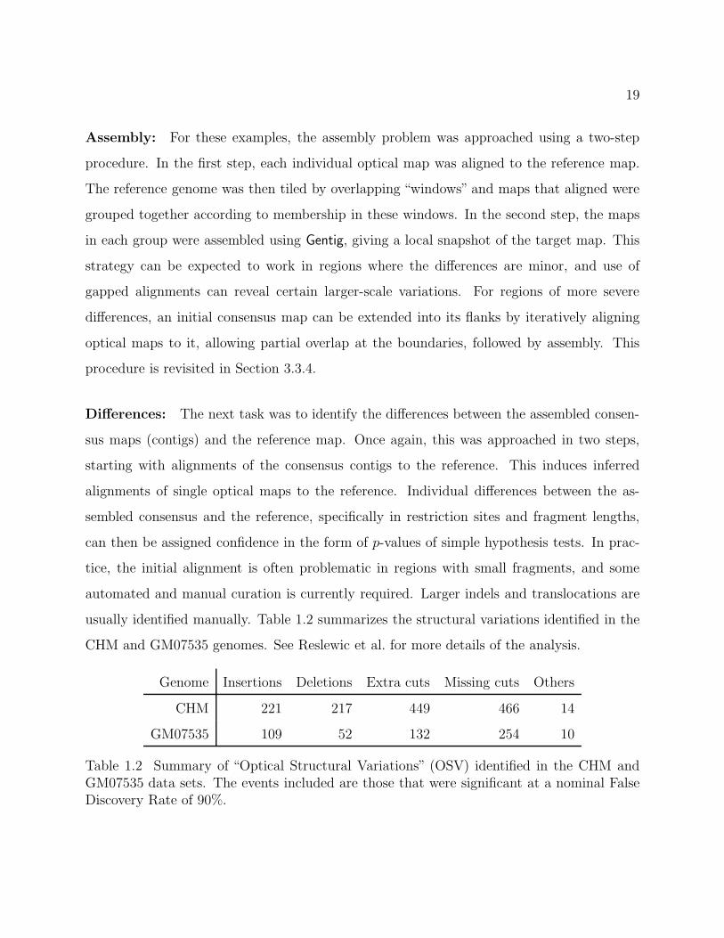
Assembly: For these examples, the assembly problem was approached using a two-step

procedure. In the first step, each individual optical map was aligned to the reference map.

The reference genome was then tiled by overlapping “windows” and maps that aligned were

grouped together according to membership in these windows. In the second step, the maps

in each group were assembled using Gentig, giving a local snapshot of the target map. This

strategy can be expected to work in regions where the differences are minor, and use of

gapped alignments can reveal certain larger-scale variations. For regions of more severe

differences, an initial consensus map can be extended into its flanks by iteratively aligning

optical maps to it, allowing partial overlap at the boundaries, followed by assembly. This

procedure is revisited in Section 3.3.4.

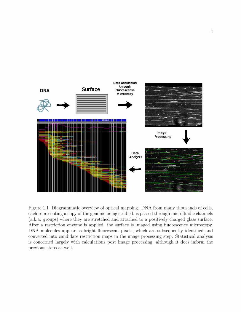
Differences: The next task was to identify the differences between the assembled consen-

sus maps (contigs) and the reference map. Once again, this was approached in two steps,

starting with alignments of the consensus contigs to the reference. This induces inferred

alignments of single optical maps to the reference. Individual differences between the as-

sembled consensus and the reference, specifically in restriction sites and fragment lengths,

can then be assigned confidence in the form of p-values of simple hypothesis tests. In prac-

tice, the initial alignment is often problematic in regions with small fragments, and some

automated and manual curation is currently required. Larger indels and translocations are

usually identified manually. Table 1.2 summarizes the structural variations identified in the

CHM and GM07535 genomes. See Reslewic et al. for more details of the analysis.

Genome Insertions Deletions Extra cuts Missing cuts Others

CHM 221 217 449 466 14

GM07535 109 52 132 254 10

Table 1.2 Summary of “Optical Structural Variations” (OSV) identified in the CHM andGM07535 data sets. The events included are those that were significant at a nominal FalseDiscovery Rate of 90%.

20

1.4 Outline

Optical mapping is a fast, low-cost, single-molecule system for producing whole genome

restriction maps. Its potential applications for studies of normal and disease biology are

manifold, but computational and statistical challenges created by large genomes must be

met in order for optical mapping to achieve this potential. Existing algorithms have been

effective on optical map data from small genomes. These algorithms do not easily extend

to the much larger data sets that are now being collected from larger genomes, and we are

as yet unable to completely mine the wealth of information contained in them. In part, this

is due to unavoidable computational bottlenecks. However, new avenues of analysis have

opened up with the availability of more and more sequence information. In the following

chapters, we present some new ideas on how to deal with optical map data. These ideas share

a common theme in that they all take advantage of the availability of in silico reference maps

derived from sequence. They do not, by any means, resolve all outstanding questions, but

hopefully they contribute to the understanding of optical map data and provide a reference

for future work in this area. In Chapter 2, we discuss stochastic models for optical map

errors and present some new approaches to parameter estimation in that setting. In Chapter

3, we propose a new method to determine significance of alignments of optical maps to a

reference, which is an important prerequisite in many analyses. In Chapter 4, we use these

alignments as the basis for an assembly-free method to detect copy number polymorphisms.

Especially in cancer biology, the ability to detect gains and losses of DNA is critical, as

frequently deleted sites may harbor tumor suppressor genes, and frequently amplified regions

may harbor oncogenes.

21

Chapter 2

Modeling Optical Map Data

The first step in the analysis of optical mapping data is to understand its inherent vari-

ability. Unlike traditional restriction mapping techniques, optical mapping obviates the need

to reconstruct the order of restriction fragments. However, the orientations of optical maps

are unknown, fragment lengths are not measured accurately, not all cuts are correctly iden-

tified, and small fragments may desorb and not be seen at all. Further, some maps identified

by image processing may not represent any real restriction maps; e.g., chimeric maps caused

by crossing over of maps in the image, marked up as one. In this chapter we discuss how

these sources of noise can be modeled. Section 2.1, which describes models for optical map

errors, is mostly a review. Later sections consider the estimation of model parameters from

optical map data. Many of the ideas presented there are new and often take advantage of

an in silico reference map. In particular, we outline a non-parametric approach to estimate

desorption rate, use alignments of optical maps to a reference to estimate sizing and scaling

error parameters, and discuss the use of simulation to develop diagnostic plots that can be

used to assess goodness of fit.

2.1 A stochastic model

2.1.1 Origin

Underlying restriction map: It is natural to model optical maps as being generated

from an underlying ‘true’ restriction map associated with the genome under study. This

restriction map can be thought of as a fixed but unknown (high-dimensional) parameter.

22

Quantiles of exponential

Qua

ntile

s of

insi

lico

frag

men

t len

gths

0

50

100

150

0 1 2 3 4 5

1 (0.12) 2 (0.08)

0 1 2 3 4 5

3 (0.09) 4 (0.06)

0 1 2 3 4 5

5 (0.09) 6 (0.08)

0 1 2 3 4 5

7 (0.09) 8 (0.09)

9 (0.1) 10 (0.09) 11 (0.1) 12 (0.11) 13 (0.06) 14 (0.1) 15 (0.08)

0

50

100

15016 (0.15)

0

50

100

15017 (0.13)

0 1 2 3 4 5

18 (0.07) 19 (0.2)

0 1 2 3 4 5

20 (0.08) 21 (0.13)

0 1 2 3 4 5

22 (0.13) X (0.08)

0 1 2 3 4 5

Y (0.08)

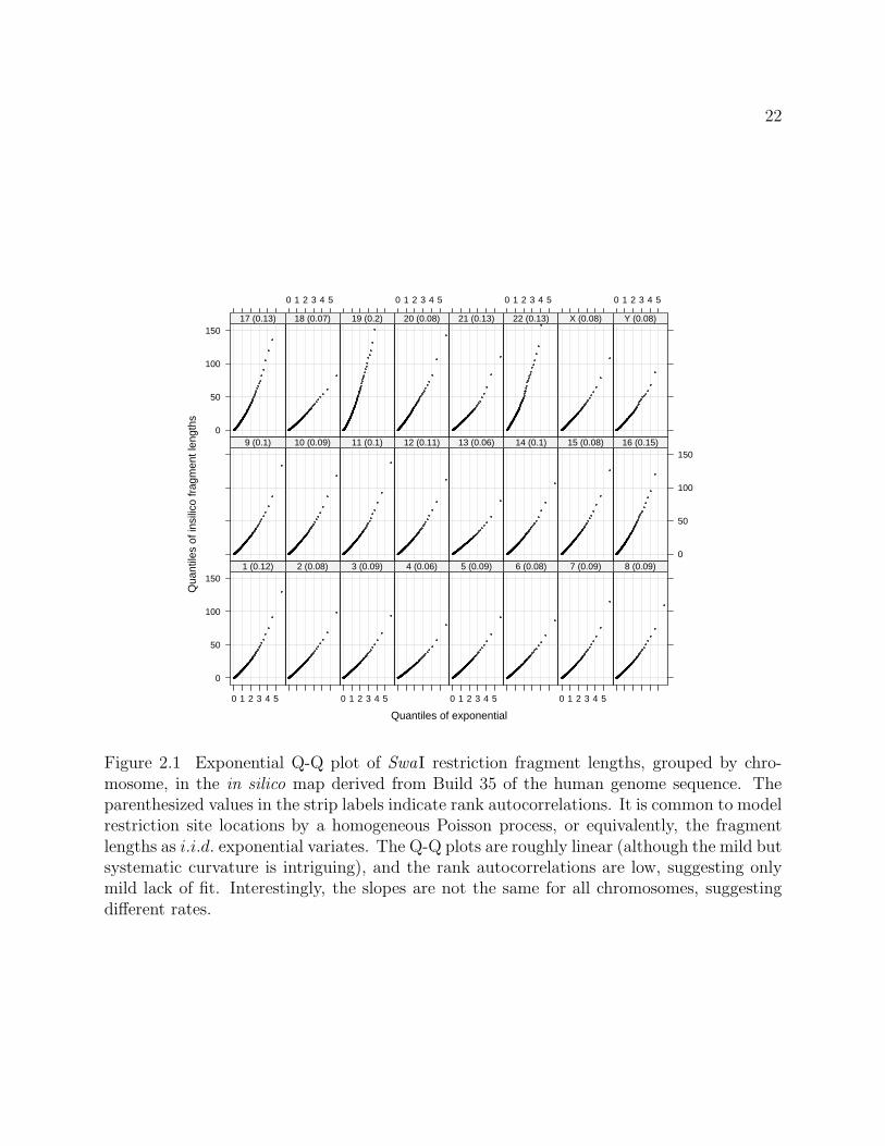
Figure 2.1 Exponential Q-Q plot of SwaI restriction fragment lengths, grouped by chro-mosome, in the in silico map derived from Build 35 of the human genome sequence. Theparenthesized values in the strip labels indicate rank autocorrelations. It is common to modelrestriction site locations by a homogeneous Poisson process, or equivalently, the fragmentlengths as i.i.d. exponential variates. The Q-Q plots are roughly linear (although the mild butsystematic curvature is intriguing), and the rank autocorrelations are low, suggesting onlymild lack of fit. Interestingly, the slopes are not the same for all chromosomes, suggestingdifferent rates.

23

Alternatively, it can be thought of as the realization of a random process; in particular,

recognition sites along the genome have been modeled as the realizations of a homogeneous

Poisson point process, or equivalently the fragment lengths as i.i.d. exponential variates. This

model is supported by Figure 2.1, derived from Build 35 of the human genome sequence.

The rate of this process depends on the restriction enzyme being used, as well as the genome

being mapped. In some cases, it may vary across, or even within, chromosomes. Genomic

differences within a species usually involve only a fraction of the genome, and corresponding

restriction maps are expected to be largely similar. In any case, we are chiefly interested in

modeling the generative process of data conditional on the underlying restriction map. It

should be noted that the notion of a ‘true’ map is somewhat simplified. Diploid genomes

have two versions of the map, largely similar but not identical. Cancer samples are usually

a mixture of several cell populations that each contribute a slightly different genome.

Shotgun breaks: Before they are passed into micro-channels, chromosomal DNA is ran-

domly broken up into smaller molecules, usually by subjecting the DNA to vibration. This

shearing is often referred to as a whole genome shotgun process. The origin of each observed

optical map molecule is characterized by its location in the coordinate system defined by the

underlying true (unknown) restriction map, as well as its length. The distribution of the

location (e.g. midpoint) is assumed to be uniform over the underlying genome. It is typical

to consider only optical maps longer than a predetermined threshold, usually 300 Kb. The

distribution of lengths of the filtered maps is usually consistent with a truncated exponential

distribution.

2.1.2 Errors

Cut site errors: A restriction site in the true restriction map may fail to show up in a

corresponding optical map. These missing cuts can be due to either incomplete digestion

by the restriction enzyme or noise in the optical map image. Whether true cut sites are

identified (success) or not (failure) is modeled as independent Bernoulli trials, with some

24

unknown probability p, say, of success. It is possible to argue that the probability should

depend on proximity to other cuts, but the idea is difficult to formalize. Instead, the issue

is dealt with using a desorption model for small fragments (see below). An optical map can

also contain false cuts, i.e. apparent restriction sites that correspond to no restriction site

in the true map, perhaps due to random breakage of DNA or image errors. The locations

of such spurious cut sites in optical maps may be modeled as the realizations of a homoge-

neous Poisson process, with rate ζ , say, per Kb of DNA. These models have been used by

Anantharaman et al. (1999) and Valouev et al. (2006).

Length measurement errors: Consider an optical map with n fragments of measured

lengths X1, . . . , Xn. Assuming no cut errors, each fragment has a corresponding true but

unobserved length, which we denote by µi, i = 1, . . . , n. Recall that each Xi is calculated as

the product YiRi, where Yi is the total fluorescent intensity of the pixels that constitute the

fragment, and Ri is a scale factor to convert fluorescent intensities to base pairs, estimated

using standards. Restricting our attention to the marginal distribution of Xi, we may treat

Yi and Ri as independent latent variables within a given image. We can assume without loss

of generality that the true scale factor is 1. It is natural to assume that the distribution of

Yi depends only on µi. Valouev et al. (2006) note that Yi is the sum of intensities of several

pixels. Assuming these terms to be i.i.d., the expected number of terms is proportional to

µi. Invoking the Central Limit Theorem, they postulate that for some σ,

Yi ∼ N(µi, σ

2µi)

This model additionally has the following desirable property: denoting the N (µ, σ2µ) den-

sity by fµ, if Yi ∼ fµi, Yj ∼ fµj

and Yi and Yj are independent, then Yi + Yj ∼ fµi+µj. This

is relevant when adjacent fragments are reported as one due to a missing cut. Valouev et al.

(2006) ignore scaling and postulate that the observed lengths Xi = Yi. If we instead as-

sume that the mean E(Ri) = 1 and variance V (Ri) = τ 2 > 0 without making any further

assumptions about the distribution of Ri, we have

E(Xi) = E(E(YiRi|Ri)) = µi

25

and

V (Xi) = E(V (YiRi|Ri)) + V (E(YiRi|Ri))

= σ2(τ 2 + 1

)µ+ τ 2µ2

In other words, the true variance is the sum of terms linear and quadratic in µ. Further,

since Yi is multiplied by a random quantity, normality of Yi may not translate to Xi. Note

that these arguments apply to the marginal distribution of Xi’s. As can be seen in Figure

1.4, fragments within a map are often much closer to each other on the surface compared to

nearby standards. Consequently, the values of Ri are likely to vary much less within maps

than between maps. In other words, fragments of an optical map are possibly correlated,

being oversized or undersized together.

Small fragments: Fragments that are relatively small add various complications to the

optical map model. Adhesion of DNA molecules to the glass surface is not overly strong,

which means that small fragments may sometimes detach and float away. This phenomenon

is referred to as desorption. It is fairly natural to model the probability of a fragment be-

ing desorbed as a decreasing function of its length. Controlled experiments suggest that this

probability reduces to 0 for fragments around 10 Kb or longer. Even when small fragments

are observed, they are often balled up instead of being clearly stretched out as longer frag-

ments. Whatever the reasons, this has the effect that the sizing error distribution described

above breaks down for smaller fragments. Generally speaking, measured lengths of smaller

fragments are believed to be more variable than the model for larger fragments would imply.

Other errors: The sources of noise described above encapsulate much of the systematic

variability observed in optical maps. There are other errors that are difficult to model, but

are present in the data nonetheless. For example, two unrelated molecules may be mistakenly

combined; these optical chimeras are particularly troublesome as they may falsely suggest

translocation in the sampled genome. Another common occurrence is for stray pieces of

fluorescent material or an intersecting map to be mistakenly considered part of a fragment,

26

resulting in an unusually large sizing error for that particular fragment. The image processing

step attempts to control such errors, but they can not be eliminated entirely.

2.2 Parameter estimation

Estimation of parameters in the stochastic model described above is difficult, but it is

important for several reasons. First, estimates of the parameters are required in certain

fundamental procedures. For example, likelihood ratio based score functions are expressed

in terms of model parameters, and exact values of the parameters are required to completely

define the score. Parameter values are also required for null distributions used in determining

p-values for potential genomic variations (Reslewic et al.). Second, estimates are necessary

in order to simulate optical maps. Due to the complex nature of the data, simulation is

often the only reasonable approach to investigate the operating characteristics of various

inferential procedures, despite the fact that the model may not capture all the variability in

real data. Simulation can also be a useful tool in directing laboratory research, since it can

provide guidance about which aspects of the experiment have the maximum impact on the

final results.

Difficulty: The difficulty in estimation arises primarily because the true restriction map

is rarely known. Even for optical maps from genomes whose sequence (and hence restriction

map) is completely known, the correspondence between cut sites in observed optical maps

and recognition sites in the true restriction map are never known with certainty. In fact,

inferring this correspondence is precisely the goal of alignment. One possibility is to assume

the correctness of alignments that are declared to be statistically significant, and then use

these alignments for estimation. We will briefly discuss such methods, noting that the

resulting estimates are likely to be biased. A secondary difficulty in estimation is due to the

fact that the parameters may not remain constant over the course of an experiment. This is

difficult to address, and we can only assume that the changes are not substantial enough to

27

affect inference. If necessary, the degree of change can be assessed by dividing the data by

time of collection and compare estimates across time periods.

To illustrate estimation techniques, we use the GM07535 data set and the in silico refer-

ence map derived from the human genome sequence (Build 35).

2.2.1 Desorption

Random truncation: We begin with the estimation of desorption rates, since this can

be achieved without alignments, under certain assumptions. For a fragment in the true

restriction map spanned by an observed optical map, let Z be a random variable indicating

whether that particular fragment was observed, and let Y be its measured length had it been

observed. The desorption rate is quantified by the probability that a fragment is observed

(not truncated), given by

π(y) = P (Z = 1|Y = y)

Suppose that the marginal density of the unobserved (pre-truncation) random variable Y is

g. Let X represent the length of an observed (truncated version of Y ) fragment, i.e. X = Y

if Z = 1. Then, the marginal density of X is given by

h(x) =1

Kπ(x) g(x)

where K is the normalizing constant

K =

∫ ∞

0

π(t) g(t) dt

As formulated, π(·) only identifiable up to scale since π′(y) := απ(y), 0 < α ≤ 1 induces the

same h from g. Desorption is known to affect small fragments only, so we may additionally

assume that limy→∞ π(y) = 1, making π(·) identifiable. Empirically, π(y) = 1 for y > 15 Kb.

Length distribution: Let us consider the distribution of the unobserved random variable

Y . Suppose the true recognition sites are realizations of a homogeneous Poisson process with

rate θ, true recognition sites are observed independently with probability p, and false cuts

28

are realizations of a homogeneous Poisson process with rate ζ . If we assume independence of

these errors and no error in sizing, then the observed cut sites are realizations of a homoge-

neous Poisson process with rate p θ+ζ . Consequently, the fragment sizes Y are exponentially

distributed. The assumption of no sizing error is of course unrealistic; Valouev et al. (2006)

show that the exponential distribution holds approximately even with reasonable sizing error

models.

Exponential rate: The rate of the relevant exponential distribution depends on unknown

parameters. Fortunately, this rate can be estimated directly from the data, thanks to the

memoryless property of the exponential distribution, namely that

P (Y > t+ s | Y > t) = P (Y > s)

when Y is exponentially distributed, or equivalently, Y |Y > t has the same distribution as

Y + t. In other words, left truncation of exponential variates is equivalent to an additive

shift. Since it is known empirically that π(y) = 1 for y > 15 Kb, the truncated observations

X|X > 15 has the same distribution as Y |Y > 15, i.e., an exponential truncated at 15 Kb.

A robust estimate of the rate can be obtained from the interquartile range of the truncated

observations. Empirical evidence is provided by a Q-Q plot of the observed values of X in

Figure 2.2.

Non-parametric estimation: A naive non-parametric estimate of π is given by

π(t) ∝ h(t)

g(t)

where h is the estimated density of observed fragment lengthsX and g is the known density of

Y . X is a positive random variable, so usual kernel density estimates are inappropriate, but

alternatives such as zero-truncated kernel density estimates and log-spline density estimates

exist. More interestingly, the non-parametric MLE of π can be obtained under the additional

assumption that π is increasing. This is reasonable since longer fragments are less likely to

desorb. The MLE follows from the existence of the MLE of a monotone density, given by

29

Quantiles of Exponential

Qua

ntile

s of

frag

men

t len

gths

(K

b)

0

5

10

15

20

25

0 5 10 15 20 25

Rate = 1 / 18.8

mean

diffe

renc

e

0.0

0.5

1.0

1.5

2.0

2.5

0 5 10 15 20 25

Rate = 1 / 18.8

Figure 2.2 Plot of quantiles of observed fragment lengths (from a subset of GM07535 opticalmaps) against quantiles of an exponential distribution. The rate is chosen so that the curveis parallel to the diagonal except near the origin. This is clearer in the second panel, which isobtained by rotating the first clockwise by 45◦. This additive shift in the Q-Q plot caused bytruncation is a feature unique to the exponential distribution that follows from its memorylessproperty.

30

Fragment length

π0.0

0.2

0.4

0.6

0.8

1.0

0 5 10 15 20 25

Figure 2.3 The non-parametric MLE of π based on the Grenander estimator. The smoothgrey curve is based on a naive zero truncated kernel density estimate of h.

the so called Grenander estimator (see van der Vaart, 1998, Chapter 24). To see this, let G

be the (known) CDF of Y . This happens to be exponential in this case, but any monotone

decreasing density is sufficient. Consider the quantities of interest in a scale transformed by

G, i.e., Y = G(Y ), X = G(X) and

π (y) = P(Z = 1|Y = y

)= π(G−1 (y))

Let h be density of X. Since Y ∼ U (0, 1) with constant density, h(x) ∝ π(x). Since G and

hence G−1 are monotone increasing transformations,

π ↑ =⇒ π = π ◦G−1 ↑ =⇒ h ↑

Hence, the MLE of h, based on Xi’s, is given by the Grenander estimator. The MLE of π is

proportional to that of h, with the constant of proportionality obtained from the fact that

limey→1 π(y) = 1. The estimator is inconsistent at y = 1, i.e. y = ∞, but that is not of

interest to us. The MLE of π in the original scale is given by π = π ◦G.

Parametric estimation: Parametric forms of π are naturally easier to work with in prac-

tice. Obtaining maximum likelihood estimates in that case is straightforward in principle;

most of the difficulty arises in obtaining the normalizing constant

K(π) =

∫ ∞

0

π(t) g(t) dt

31

as a function of the parameters. An analytical solution exists for some simple families,

including one that is commonly used, given by πα(t) = 1 − e−αt, α > 0.

Caveats: Although the analysis described above is appealing, it depends critically on the

assumption that Y is exponentially distributed, which in turn depends on the sizing error

model used. Unfortunately, sizing error is less stable for small fragments, which is precisely

the region of interest. It should also be noted that even if the exponential distribution

holds marginally, fragment lengths can be considered independent only conditional on the

underlying restriction map. The marginal dependence is weak for large genomes, but cannot

be ignored for smaller ones.

2.2.2 Length errors

Parameters: Recall that the marginal distribution of the measured length of an optical

map fragment of true length µ is characterized by mean µ and variance σ2 (τ 2 + 1)µ+τ 2µ2. σ

and τ can be estimated indirectly given a reasonable alignment scheme, provided we assume

highly significant alignments to be true. The values of σ and τ used in Figure 2.4 were

derived using an informal method of moments estimator, with the observed variances for

subsets of the data defined by various ranges of µ used as the response in a linear regression

with terms µ and µ2. It should be noted that these estimates are based on maps with

significant alignments and are thus likely to be biased to some extent.

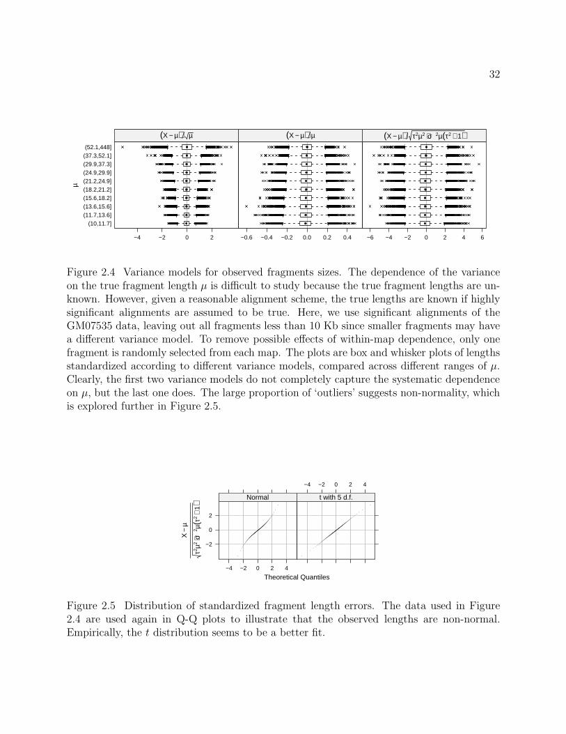
Normality: Figure 2.4 suggests that the distribution of the standardized lengths have

heavier tails than normal. This is clearer in the normal Q-Q plot in Figure 2.5. Empirically,

a t distribution appears to be a much better fit, which is not surprising since the calculation

of Xi involves an estimated scale (see Section 2.1.2).

2.2.3 Cut errors

The probability p of a true cut being observed and the rate ζ of spurious cuts can be

similarly estimated using significant alignments. However, the amount of bias introduced

32µ

(10,11.7](11.7,13.6](13.6,15.6](15.6,18.2](18.2,21.2](21.2,24.9](24.9,29.9](29.9,37.3](37.3,52.1](52.1,448]

−4 −2 0 2

(X − µ) µ

−0.6 −0.4 −0.2 0.0 0.2 0.4

(X − µ) µ

−6 −4 −2 0 2 4 6

(X − µ) τ2µ2 + σ2µ(τ2 + 1)

Figure 2.4 Variance models for observed fragments sizes. The dependence of the varianceon the true fragment length µ is difficult to study because the true fragment lengths are un-known. However, given a reasonable alignment scheme, the true lengths are known if highlysignificant alignments are assumed to be true. Here, we use significant alignments of theGM07535 data, leaving out all fragments less than 10 Kb since smaller fragments may havea different variance model. To remove possible effects of within-map dependence, only onefragment is randomly selected from each map. The plots are box and whisker plots of lengthsstandardized according to different variance models, compared across different ranges of µ.Clearly, the first two variance models do not completely capture the systematic dependenceon µ, but the last one does. The large proportion of ‘outliers’ suggests non-normality, whichis explored further in Figure 2.5.

Theoretical Quantiles

X−

µ

τ2 µ2+

σ2 µ(τ2

+1)

−2

0

2

−4 −2 0 2 4

Normal

−4 −2 0 2 4

t with 5 d.f.

Figure 2.5 Distribution of standardized fragment length errors. The data used in Figure2.4 are used again in Q-Q plots to illustrate that the observed lengths are non-normal.Empirically, the t distribution seems to be a better fit.

33

by rejecting maps that do not align, as well as assuming that the significant alignments are

completely correct, is uncertain. Often it is instructive instead to assess a model by some

diagnostic plots, as described next.

2.3 Diagnostics

Due to the complexity of the model and the interplay between its various aspects, it is

next to impossible to estimate all the parameters separately. However, given a particular

set of parameter values, maps simulated from that model can be used to indirectly test

goodness of fit. Specifically, simulated maps should have characteristics that are similar to

observed maps, be they numerical summaries or graphical diagnostics. In Figures 2.6, 2.7

and 2.8, we present three diagnostic plots based on the marginal distributions of observed

restriction fragment lengths, and the number of fragments in a map. The data being modeled

is the set of GM07535 optical maps; maps are simulated from the in silico reference map

with a combination of values for p (0.70, 0.75 and 0.80) and ζ (0.001, 0.003 and 0.005),

keeping all other components fixed. The rate of desorption is determined by the function

πα(t) = 1− e−αt. The first plot suggests that the effect of desorption has been well modeled.

Considered together, the three plots suggest that p = 0.7 and ζ = 0.005 come closest to

modeling the observed data. It is important to note that these are only a few examples,

and other similar diagnostic plots could be useful for similar purposes. None of these plots

require alignments, but plots analogous to Figure 2.4 that do depend on alignment may also

be useful.

34

Quantiles of fragment lengths in simulated data

Qua

ntile

s of

GM

O75

35 fr

agm

ent l

engt

hs

0

50

100

150

200

250

0 50 100 150 200 250

0.700 − 0.001 0.750 − 0.001

0 50 100 150 200 250

0.800 − 0.001

0.700 − 0.003 0.750 − 0.003

0

50

100

150

200

2500.800 − 0.003

0

50

100

150

200

2500.700 − 0.005

0 50 100 150 200 250

0.750 − 0.005 0.800 − 0.005

Figure 2.6 Diagnostic plots based on the distribution of observed optical map fragmentlengths. This is similar in principle to Figure 2.2, and in fact has the same quantities onthe vertical axis, namely the quantiles of observed fragment lengths of GM07535 opticalmaps. However, instead of quantiles of exponential, the horizontal axis here has quantilesof fragment lengths in optical map sets simulated using various combinations of parametervalues. The effect of desorption appears to have been modeled fairly well. The spuriouscut rate ζ appears to have little effect (at least for the values used here), but the digestionprobability p certainly does.

35

mean

diffe

renc

e

−10

0

10

20

30

0 50 100 150 200 250

0.700 − 0.001 0.750 − 0.001

0 50 100 150 200 250

0.800 − 0.001

0.700 − 0.003 0.750 − 0.003

−10

0

10

20

300.800 − 0.003

−10

0

10

20

300.700 − 0.005

0 50 100 150 200 250

0.750 − 0.005 0.800 − 0.005

Figure 2.7 As we saw in Figure 2.2, it is often helpful to look at rotated Q-Q plots so thatdeviations from the diagonal are emphasized. In this mean-difference plot, which effectivelyrotates each panel in Figure 2.6 clockwise by 45◦, systematic patterns are apparent that werenot obvious in the earlier plot. In particular, this plot gives more insight into the subtlereffect of the spurious cut rate. Recall that the distribution of fragment lengths is roughlycomparable to an exponential distribution with mean 20 Kb, so more than 99% of fragmentsare shorter than 100 Kb.

36

x

P(X

=x)

0.00

0.05

0.10

0.15

0.20

10 20 30 40 50 60

0.700 − 0.001 0.750 − 0.001

10 20 30 40 50 60

0.800 − 0.001

0.700 − 0.003 0.750 − 0.003

0.00

0.05

0.10

0.15

0.20

0.800 − 0.003

0.00

0.05

0.10

0.15

0.20

0.700 − 0.005

10 20 30 40 50 60

0.750 − 0.005 0.800 − 0.005

Figure 2.8 A hanging rootogram comparing the observed distribution of the number offragments in GM07535 optical maps to various simulated map sets. The rootogram, aninnovation due to John Tukey, is intended to compare the distribution of a discrete randomvariable to a reference distribution. Here, the continuous reference curve represents therelative frequencies of number of fragments observed in the GM07535 data and is the samein each panel. The vertical lines represent corresponding frequencies in simulated data, butthey ‘hang’ from the reference rather than starting from the origin. Systematic departuresfrom the reference are indicated by patterns of the lower endpoints relative to the origin.Also, the vertical axis plots the square root of the proportions (hence the name rootogram)to emphasize smaller probabilities.

37

Chapter 3

Significance of Optical Map Alignments

3.1 Introduction

Physical maps describe the locations of one or more markers on a genome and can be

viewed as a coarse summary of the full DNA sequence. Restriction maps are physical maps

induced by restriction enzymes, naturally produced by bacteria to defend themselves by

cutting up (or restricting) foreign DNA. The marker associated with a restriction enzyme

is a specific pattern it recognizes and cleaves; typically a palindromic DNA sequence 4 to 8

base pairs long. Optical mapping (Schwartz et al., 1993; Dimalanta et al., 2004) is a single

molecule approach for the construction of ordered restriction maps of genomic DNA. DNA

molecules broken apart using a shotgun process are stretched and attached to a positively

charged glass support. When a restriction enzyme is applied, it cleaves the DNA at sites

recognized by the enzyme. The DNA molecules remain attached to the surface, but the

elasticity of the stretched DNA pulls back the molecule ends at the cleaved sites. After

being stained with a fluorochrome, these sites can be identified under a microscope as tiny

gaps in the fluorescent line of the molecule, giving a local snapshot of the full restriction

map.

Noise: Unlike other restriction mapping techniques, optical mapping bypasses the problem

of reconstructing the order of the restriction fragments. However, optical map data are not

perfect: the inter-site fragment sizes are not measured exactly, some true recognition sites

may go undigested by the enzyme or unidentified by image processing, some spurious cuts

38

may appear where there should have been none and small fragments may not be represented

because they float away or merge with neighboring fragments. See Chapter 1 for a detailed

overview of the optical mapping system and Chapter 2 for more on the inherent errors and

statistical features of optical map data.

Alignment: A fundamental computational problem in optical mapping is alignment, i.e.,

given an optical map, trying to identify whether it overlaps with other restriction maps, and if

so, where. Alignments are not particularly valuable individually, but used en masse they are

important components in many procedures. Dynamic Programming (DP) algorithms have

been used extensively in DNA and protein sequence alignment (Durbin et al., 1998), and can

be used to align restriction maps with suitable modifications (Huang and Waterman, 1992).

Dynamic programming is a generic approach to alignment, and its usefulness depends on the

details of how it is applied. There are two important components in such alignment schemes.

The first is a score function, which is the objective function that the algorithm maximizes

(see Appendix A). The second is the strategy for detecting significance, i.e., whether or not

the alignment with the optimum score, which exists even if there is no true alignment, should

be considered a real alignment as opposed to a spurious one. The nature of optical mapping

data makes this problem harder than for sequence alignment.

Significance: Prior to the present work, the detection of significance in optical map align-

ments has not been systematically studied. Conceptually, the problem is a test for the null

hypothesis that the maps being aligned are independent, with the optimal score as the test

statistic. Unfortunately, the null distribution, i.e. the distribution of the optimal score under

independence, is not easy to obtain. Rules based on simulated optical maps are possible;

however, they are predicated on the accuracy of the simulation model, which may not truly

reflect all the complexities of optical mapping. Our main contribution, as described in Sec-

tion 3.2, is to phrase the significance problem in a way that allows us to naturally sample

from the null distribution of optimal scores avoiding any explicit model for optical maps. In

Section 3.3, this framework is used to investigate the properties of a particular score function

39

using optical mapping data from a human genome. Finally, we consider the implications of

the proposed approach in Section 3.4. Among other things, we develop conditional signifi-

cance tests with control over error rates, outline a scheme to compare various score functions

and provide explanations for several empirical observations.

3.2 Methods

Alignment problems are primarily of two kinds; first, where an optical map is aligned

against another optical map, and second, where an optical map is aligned against an error-

free reference map, typically derived in silico from sequence. The first kind might be a

component in assembly algorithms. The second kind can be used to divide a large assembly

problem, which are at least of quadratic complexity, into smaller tractable ones (see Section

1.3.5). Here, we restrict our attention to alignment problems of the second kind. Such

alignments are also used in Chapter 4 to investigate copy number alterations.

Formulation: Denote an optical map by M and the in silico reference map by G. Consider

scores for all possible alignments of M to G and choose the alignment for which the score is

maximized. Denote the corresponding optimal score by S. We are interested in determining

whether this optimal alignment is statistically significant. It is convenient to phrase this

question as a test of independence. Specifically, it is assumed that M and G are random

quantities generated by some stochastic mechanism, and the statistic S is used to test the

null hypothesis H0 : M ⊥ G. The distribution of S under H0 is determined by the marginal

distributions of M and G.

Conditional permutation test: We avoid specification of the distribution of M, which

is complex, by conditioning on M. Let PG denote the marginal distribution of G. For any

random G ∼ PG, let S(G|M) be the optimal score obtained by aligning the fixed M against

G. PG induces a distribution of the scalar random variable S(G|M), represented by the

corresponding CDF, denoted F0(·|M). Using the observed optimal score S = S(G|M

), H0

40

is rejected at level α if S > cα where F0(cα|M) = 1 − α. The advantage of this formulation

is that given a choice of PG, we can in principle simulate from F0(·|M) to obtain a suitable

cutoff, without requiring any probabilistic model for the optical map M. An effective choice

of PG is given by random permutations of the reference G. This preserves characteristics of

the reference that are known to affect the spurious score distribution, namely the number

and lengths of fragments. Permuting the order of fragments is also reasonable given the

additive nature of score functions, which essentially reward matches in order. Formally, if we

assume that the fragment lengths defining G are i.i.d. from some distribution in a family F ,

permutation can be viewed as sampling from PG conditional on the set of fragment lengths in

G, which is sufficient for F . Such tests are often called permutation tests (Cox and Hinkley,

1979, Chapter 6). See Figure 3.1 for a graphical justification of the i.i.d. assumption.

3.3 Results

3.3.1 Exploration

We use optical map data from GM07535, a diploid normal human lymphoblastoid cell line,

for illustration. The data consists of 206796 optical maps longer than 300 Kb. These maps

are aligned against an in silico reference map derived from Build 35 of the human genome

sequence (International Human Genome Sequencing Consortium, 2004), with sequence gaps

replaced by their estimated length. We use a score function implemented in the SOMA

software suite with parameters that have been extensively used with optical map data. The

actual score function, henceforth referred to as the SOMA score, is described in Appendix

A. In addition to the best alignment scores against the in silico reference, we consider best

scores for each map against several independent random permutations of the reference. The

permutations are done separately for every chromosome, thus retaining the total length and

number of fragments within each. For the most part, we restrict our attention to ungapped

global alignments.

In theory, we can approximate the conditional null distribution F0(·|M) by sampling from

it an arbitrary number of times. In practice, each such sample involves a permutation of

41

Pairs of successive ranks

0.0

0.2

0.4

0.6

0.8

1.0

0.0 0.2 0.4 0.6 0.8 1.0

chr1 ( 0.12 ) chr2 ( 0.08 )

0.0 0.2 0.4 0.6 0.8 1.0

chr3 ( 0.09 ) chr4 ( 0.06 )

0.0 0.2 0.4 0.6 0.8 1.0

chr5 ( 0.09 ) chr6 ( 0.08 )

chr7 ( 0.09 ) chr8 ( 0.09 ) chr9 ( 0.1 ) chr10 ( 0.09 ) chr11 ( 0.1 )

0.0

0.2

0.4

0.6

0.8

1.0chr12 ( 0.11 )

0.0

0.2

0.4

0.6

0.8

1.0chr13 ( 0.06 ) chr14 ( 0.1 ) chr15 ( 0.08 ) chr16 ( 0.15 ) chr17 ( 0.13 ) chr18 ( 0.07 )

chr19 ( 0.2 )

0.0 0.2 0.4 0.6 0.8 1.0

chr20 ( 0.08 ) chr21 ( 0.13 )

0.0 0.2 0.4 0.6 0.8 1.0

chr22 ( 0.13 ) chrX ( 0.08 )

0.0 0.2 0.4 0.6 0.8 1.0

0.0

0.2

0.4

0.6

0.8

1.0chrY ( 0.08 )

Figure 3.1 Independence of in silico fragment lengths. Our method presumes that re-striction fragment lengths in the reference copy are i.i.d.. Here, we plot successive pairs ofranks separately for each chromosome. The scatter is fairly uniform, supporting the i.i.d.assumption. The figures in parentheses indicate rank autocorrelation. The average frag-ment length is known to differ across chromosomes, so we restrict all permutations to withinchromosomes.

42

Spurious scores

Replication 1

Rep

licat

ion

2

−15

−10

−5

0

5

−15 −10 −5 0 5

Counts

1133978

132199280374482604740889

10521229142016241842

Figure 3.2 Dependence of spurious scores on optical map. For each map, the optimal scoresfor ungapped global alignment against two independent permutations of the reference areplotted against each other. The scores are highly correlated, suggesting that a significantcomponent of the distribution of the best spurious score for an optical map is determined bythe map itself.

the reference map followed by alignment. The large number of maps and the computational

cost of alignment makes this approach undesirable, and leads us to search for methods in

which a limited number of permutations suffice. Figure 3.2, which uses hexagonal binning

(Carr et al., 1987) to plot the optimal scores of each map against two independent permu-

tations of the reference, suggests that F0(·|M) depends strongly on the map. This insight

provides ways to substantially simplify the map-specific assessment of significance. We can

express the optimal “spurious” scores S(G|M) as

S(G|M) = µ(M) + ǫ(G|M) (3.1)

where µ(M) is a map-specific mean and ǫ(G|M)’s are independent deviations with mean 0.

As specified, this is a trivial model which is only useful with further assumptions. In view

of Figure 3.2, it is not unreasonable to suppose that the distribution of ǫ(G|M) is free of M,

or perhaps depends on it only through µ(M). We can proceed either by estimating µ(M)

separately for each map, or by postulating a functional form for µ(M). Both approaches are

useful and are discussed in turn.

43

3.3.2 Simplifications

Direct approach: If the deviations ǫ(G|M) are i.i.d., then for G1 and G2 independent

realizations from PG, the difference T (M) = S(G1|M) − S(G2|M) has distribution free of

M. This allows us to indirectly check distributional assumptions on ǫ(G|M). For example, if

ǫ(G|M) ∼ N (0, σ2) then T ∼ N (0, 2σ2). Since the scores are extreme values, a more natural

model for ǫ(G|M)’s is a scale and location shifted Gumbel distribution, in which case T has

a logistic distribution (Gumbel, 1961). Figure 3.3 shows Q-Q plots of observed differences

against both distributions, suggesting that the latter model is more plausible. More generally,

with optimal scores for each map against n independent permutations from PG, we can define

the test statistics S(G|M

)− µ (M) with mean 0 and variance

(1 + 1

n

)V ar(ǫ(G|M)) under

the null, where

µ (M) =1

n

n∑

i=1

S (Gi|M)

In practice, the i.i.d. assumption is not entirely justified. Rather, as Figure 3.4 suggests, a

model with standard deviation linear in µ(M) is more appropriate, e.g.:

V ar(ǫ(G|M)) = σ2(δ1 − µ(M))2

δ1 can be estimated using Iteratively Reweighted Least Squares to fit a suitable generalized

least squares model, to give standardized test statistics

T1 (M) =S

(G|M

)− µ (M)

δ1 − µ (M)

Cutoffs can be estimated empirically; each optical map aligned to a further independent

permutation of the reference provides a single sample from the null distribution.

Regression: A second approach is to model µ(M) as a parametric function of M. A

simple scheme that appears to work well is multiple linear regression with the number of

fragments in a map and its length in base-pairs as predictors. For each map, µ (M) is an

unbiased estimator of µ(M) and can serve as the response in the regression model. Figure

44

Theoretical quantiles

Qua

ntile

s of

diff

eren

ce

−10

−5

0

5

10

−4 −2 0 2 4

Normal

−10 −5 0 5 10

Logistic

Figure 3.3 The distribution of ǫ(G) induces a distribution of the difference between twoindependent realizations of the best spurious score for a map. This distribution can becompared to observed data to indirectly check models for ǫ(G). The Q-Q plots here suggestthat a logistic distribution for the differences (induced by an extreme value distribution forǫ) is a better fit that normal (induced when ǫ’s are normal).

Average spurious score

Abs

olut

e de

viat

ion

from

ave

rage

0

1

2

3

4

5

6

−40 −30 −20 −10 0

Counts

1113263

105158221295380475582698826964

111312731443

Figure 3.4 Variance of errors. µ(M) is estimated by the average spurious score against fourpermutations from PG. Absolute deviations of scores against a fifth permutation is plottedagainst these averages. The LOESS smooth suggests that the standard deviation of theerrors is a linear function of the average spurious score.

45

Mea

n sp

urio

us s

core

−20

−10

0

20 40 60

Number of fragments

400 600 800 1000

Length (Kb)

−30 −20 −10 0

Regression Fit Counts

136

122259445683971

1309169821382628316937604402509458376630

Figure 3.5 Parametric models for µ(M). The average of four spurious scores for each map isplotted against the number of fragments N , the length L, and the fitted values from a linearmodel with terms N , L and their product NL. The multiple regression model explains moreof the variability, and also suggests better symmetry.

3.5 demonstrates the utility of this approach. As before, a generalized least squares model

with standard deviation linear in the fitted values is more appropriate, giving standardized

test statistics

T2 (M) =S

(G|M

)− µ (M)

δ2 − µ (M)

where µ (M) are the fitted responses.

Comparison: Table 3.1 summarizes the results from both approaches. Specifically, the

mean spurious scores for each of the 206796 GM07535 maps were estimated using n = 4

permutations of the reference. A fifth permutation was used for parameter estimation: δ1

in the direct approach, δ2 and the regression coefficients in the regression approach. A sixth

permutation was used to sample from the null distributions, and 99% and 99.9% cutoffs

were determined by the appropriate quantiles of these samples of size 206796. The two

approaches largely agree in both cases. For aligning a future map, the regression method

is of more practical value, as it would require only one alignment to G, whereas the direct

method would require additional alignments to several permuted references to estimate µ(M).

46

Nominal specificity: 99.0%

Regression

Direct Not significant Significant

Not significant 63.3 2.3

Significant 2.9 31.6

Nominal specificity: 99.9%

Regression

Direct Not significant Significant

Not significant 72.9 1.1

Significant 2.8 23.2

Table 3.1 Percentage of GM07535 maps (out of 206796) declared significant by the twomethods. The direct approach makes fewer assumptions, although its precision can be furtherimproved by using more permutations. The regression approach is an approximation thatseems to perform well, which is welcome news as the latter is of more practical value. SeeFigure 3.12 and the accompanying discussion for more on this topic.

47

3.3.3 Simulation

Given a generative model, such as the one described in Chapter 2, we can simulate optical

maps and align them using the test developed above. Since we know the origin of these maps,

we can estimate the true sensitivity and specificity. Such models are of limited use since they

do not capture all the sources of noise in real data, nor do they reflect the fluctuations in

parameter values that occur in the course of a real experiment. Nonetheless, simulation is

a valuable diagnostic tool. We applied the regression test derived above with a nominal

specificity of 99.9% to 50,000 maps simulated from the human reference. 73.42% of correct

alignments were declared as significant, 0.39% had at least one spurious alignment declared

to be significant in addition to the correct one and 0.27% had only spurious significant

alignments. It should be noted that some incorrect alignments are likely to be legitimate

due to repeat structures in the genome.

3.3.4 Improving assembly

Alignments of optical maps to a reference is an important component of the iterative as-

sembly scheme described in Section 1.3.5. Previously, a constant cutoff (determined heuris-

tically) has been used to assess significance with the SOMA score. Figure 3.2 clearly suggests

that this can be improved. By replacing the constant cutoff with the rules derived above and

comparing the results, we can get quantitative validation of our methods indirectly through

assembly. Figure 3.6 compares the results of using various significance strategies, includ-

ing the previously used cutoff and two regression cutoffs with different nominal specificities.

Chromosome 2 was assembled using the CHM data set (Section 1.2), which was not used in

determining the significance rules. A simple measure of success is the contig rate, i.e., the

proportion of maps passing the alignment step that are eventually included in the assembly.

By this measure, the new strategy clearly performs better. It is less clear how to compare

the quality of the resulting alignments, but the few measures we use in Figure 3.6 also favor

the new significance strategy.

48

Iteration

8000

10000

12000

140002Number Input

7000

8000

9000

10000

2Number in assembly

0.70

0.75

0.80

0.85

0.90

0.95

2Ratio

226

228

230

232

1 2 3

2Bases Covered (Mb)

15

20

25

30

1 2 3

2Number of Gaps

0.004

0.006

0.008

0.010

0.012

1 2 3

2Proportion Unaligned

Constant (4.5 / 10)Constant (2.75 / 10)

Regression (99.9 %)Regression (99.0 %)

Figure 3.6 Comparison of various significance strategies through the iterative assemblyprocedure of Reslewic et al., where pairwise alignment is used as a filtering step before as-sembly. Chromosome 2 is assembled using the CHM data and the SOMA score. Two versionsof the regression-based cutoff, with nominal specificities of 99.9% and 99.0%, are comparedwith a previously used scheme of declaring significance when the alignment has more than10 aligned restriction sites and score above 4.5. To investigate whether performance is onlyaffected by the number of maps allowed in by the filter, a similar scheme with the constantcutoff lowered to 2.75 is also used, where the cutoff is selected to allow roughly the samenumber of maps in the first step as the 99.0% regression cutoff. To allow partial alignmentsat the boundary of the reference, “aligned length” and “count” are used as surrogates forlength and number of fragments, which effectively make the regression cutoffs more conser-vative than their nominal specificities would suggest. The first row reports the number ofmaps fed into the assembly step and the number (and proportion) of these assembled intocontigs. In the second row, we attempt to assess the quality of the assembly by aligning theconsensus contigs to the original in silico reference. The first two panels graph the numberof bases in the reference covered and the numbers of gaps. The third panel shows a crudemeasure of the false positive rate, namely the proportion of bases in the assembled contigsthat do not align to the reference.

49

3.4 Discussion

3.4.1 Uses

Alignment is a fundamental problem in optical mapping. From a statistical perspective,

optical map alignment is more challenging than DNA sequence alignment because optical

map data are more noisy. Prior work in this area has mostly focused on developing score

functions that can be used in DP algorithms. Here we have proposed a general framework to

study the null distributions of optimal scores for an arbitrary score function. Its most obvious

use is to derive significance tests with direct control over error rates. We have demonstrated

the usefulness of such tests in improving assembly of large genomes.

Evaluating score functions: The methods described above are applicable to any score

function and provide a natural mechanism to evaluate them. We consider here the model-

based likelihood ratio (LR) score proposed by Valouev et al. (2006) for aligning optical maps

to an in silico reference. Figure 3.7 plots the best spurious ungapped global alignment score

against two replications from PG using this score. The correlation is weaker, but a map

specific cutoff is still more appropriate than a constant cutoff. We apply the direct approach

as before with n = 4 replications to estimate µ(M). The results, shown in table 3.2, indicate

that at least for the particular sets of parameters used, the SOMA score is more sensitive at a

comparable specificity. This is somewhat surprising, since the LR score is based on a formal

likelihood ratio test whereas the SOMA score is largely heuristic. Informal experiments

suggest that this is at least in part due to the sizing model used by Valouev et al. (2006),

which does not consider scaling errors and consequently underestimates the marginal sizing

variance for large fragments.

More generally, this framework can be used for exploratory purposes, e.g. to compare the

performance of different scores, or to guide the choice of parameters for a given score. It is

helpful, particularly for overlap alignments (required in iterative assembly to extend flanks

of a contig), if the distribution of the optimal score under the null does not depend strongly

on the map, since otherwise significant alignments can be masked by spurious alignments.

50

Spurious score

Replication 1

Rep

licat

ion

2

20

30

40

50

60

70

20 30 40 50 60 70

Counts

1123468

114172241322415520636764904

1056121913941581

Figure 3.7 LR scores for ungapped global alignment, after Valouev et al. (2006). Optimalscores for GM07535 optical maps aligned against two independent permutations of the insilico reference are plotted against each other.

Nominal Specificity

Score function 99.0% 99.9%

SOMA 34.47 26.01

LR 26.09 18.84

Table 3.2 Percentage of GM07535 maps declared as significant by the SOMA and LR scoresusing the direct approach.

51

The ability to simulate from the null distribution allows us to try out and choose from

among various sets of parameters. Note that an appropriate choice may depend on the task;

for example, the best score for gapped alignment is always larger than that for ungapped

alignment, so the same set of parameters may not be optimal for both. Indeed, it is tempting

to try and ‘improve’ the scores we have used in our examples and consider ones other than

those reported in Table 3.2; however, we will refrain from doing so since a proper study

requires a systematic effort that is beyond the scope of this discussion.

3.4.2 Information measure

Location-specific cutoff: It is empirically known that different cutoffs for the SOMA

score seem appropriate for alignments to different parts of a reference map, but a formal ap-

proach incorporating this idea has been difficult to formulate. Map-specific cutoffs provide

a perfectly natural explanation for this observation, since an optical map is largely deter-

mined by its origin. However, this does not guard against spurious alignments at similar

(homologous) regions in the genome, which are also a potential concern.

Information measure: A related construct that proves useful in further understanding

optical map score functions is the score obtained by aligning a map with itself, which we

henceforth denote by ψ(M). Given a score function, this can be thought of as an information

measure for the map: if the map had no errors, this would be the score for the correct align-

ment. Errors normally reduce the correct alignment score from this perfect score. ψ(M) is of

course higher for longer maps, but is also affected by the lengths of the component fragments

since most score functions reward matches involving longer fragments, which are rarer. Maps

with lower information content are naturally harder to align successfully. However, Figure

3.8 shows that even for maps with high information content, the distributions of spurious

and real SOMA scores are not well separated.

Simulation: In general, any optical map dataset and score function can be summarized

by a plot analogous to Figure 3.8. Figure 3.9 shows such a plot for a set of simulated optical

52

self−alignment score

Opt

imal

sco

re

−20

−10

0

10

20

10 20 30 40

Real

10 20 30 40

Permuted Counts

110285591

136191254327409499599708827954

10901236

Figure 3.8 Optimal scores with the real and a permuted reference map are plotted for eachoptical map against alignment score with itself. The solid diagonal line represents the idealscore for a map, had it been completely error free.

53

maps, where the separation between spurious and real scores is much more clear. Comparison

with Figure 3.8 reveals an interesting point, namely that for a fair proportion of real optical

maps with high information content, the optimal score with the real reference is more likely

to have risen from the spurious score distribution than the real one. This could be due to

the maps being of low quality, but could also be a reflection of real differences between the

reference map and the actual genome. Maps of the latter type are of particular interest as

they contain possibly novel information about the underlying genome. This fact can be used

to develop a filter to obtain a smaller subset of maps relatively richer in “interesting” maps.

One possible approach to calibrate such a filter is described below. The usefulness of such

filters is yet to be explored.

Thinning: Even if all declared alignments were correct, the set of inferred locations would

only be a subset of the full set of true shotgun locations because not all maps are successfully

aligned. The probability that a map will be successfully aligned depends on the origin of the

map, its length and the errors involved (Figure 3.10). Averaging out the length and error

distributions, this probability can be expressed as a location specific truncation probability.

This random truncation can be thought of as a thinning of the true coverage process, which is

usually modeled as a homogeneous Poisson process (Lander and Waterman, 1988). A good

estimate of the thinning rate is necessary to normalize observed coverage, which can, for

example, be used to study copy number alterations in the underlying genome (Chapter 4).

This estimation has traditionally been done by Monte Carlo simulation of noisy maps from

a normal reference map, followed by alignment, thus replicating the pipeline actual optical

maps go through. The most time consuming step in this process is alignment. In view of the

discussion above, we may expect to be able to model the probability of a map being aligned

as a function of ψ(M). In particular, for the SOMA score and ungapped global alignment,

we fit the following logistic regression model to the alignments of simulated maps used in

Figure 3.9:

P ( aligned | M ) =eα+β logψ(M)

1 + eα+β logψ(M)(3.2)

54

self−alignment score

Opt

imal

sco

re

−20

−10

0

10

20

10 20 30 40

Real

10 20 30 40

Permuted Counts

149

16243547627897

117139163189217247279

Figure 3.9 Analogue of Figure 3.8 for 50000 simulated optical maps, where the best alignmentscore for real and permuted reference maps are plotted against ψ(M). Possible explanationsfor the differences between this and the previous plot are discussed in the text.

55

Figure 3.10 Schematic representation of“thinning”in optical map alignments. The horizontalaxis represents the underlying genome, with vertical lines indicating restriction sites. Onthe left, optical maps are represented as intervals, while on the right they are viewed aspoint events represented by the midpoint of the optical maps. The top panel in both plotsrepresent the true shotgun random sample of optical maps that originated from this region.Actual optical maps obtained by image processing will have noise, including sizing errors,missing cuts and false cuts, so not all these maps will be successfully aligned. Further, thechance of being aligned may depend on the location of the map; for example, maps withfewer fragments (from regions with fewer recognition sites) may be less likely to align thanmaps of similar length with more fragments. In the bottom panels, which represent theresults of alignment, unaligned maps are indicated in grey. We ignore any possible errorsin the alignment step, assuming that they would be mild. Since the probability of beingsuccessfully aligned depends on the origin, the locations of aligned maps, which is what weactually observe, are no longer uniformly distributed.

56

Location (Mb)

Den

sity

0.000

0.005

0.010

0.015

20 25 30 35 40 45 50

0.000

0.005

0.010

0.015

50 55 60 65 70 75

0.000

0.005

0.010

0.015

75 80 85 90 95 100 105

Actual alignments Predicted by model

Figure 3.11 Estimated thinning rates. The data are approximately 10,000 simulated mapsfrom human chromosome 14. The first curve is the kernel density estimate of locationsobtained from alignments declared significant. The second curve is the density of the truelocations of the same simulated maps, but with weights given by model (3.2).

The fitted model was then used to estimate P ( aligned | M ) for a new set of maps simulated

from chromosome 14, which were actually aligned as well. Figure 3.11 compares the kernel

density estimate obtained from aligned locations with the estimated density of the true

locations of all simulated maps, but with weights given by model (3.2). The estimated

densities estimated by the two methods are very close, suggesting that we can do away with

the alignment step without substantial drawbacks.

The calibration provided by (3.2) can also help in preliminary filtering of optical maps.

Currently, it is common to entirely remove maps shorter than a certain length (typically 300

Kb) from analysis as they are expected to have little information. Our observations would

suggest that ψ(M) is a better quantity on which to base this decision. This is also related to

our earlier discussion motivated by a comparison of Figures 3.8 and 3.9. The subset of maps

that have a high probability of being aligned based on ψ(M) but are not actually aligned to

the reference are likely to contain a higher proportion of maps that originate from regions of

the genome not represented in the reference copy.

3.4.3 Other topics

Choice of Null hypothesis: Independence of M and G is not necessarily the obvious

hypothesis to test when determining significance. It is not unlikely for an optical map,

57

especially a short noisy one, to originate from somewhere in the reference but have its

optimal alignment somewhere else. The null hypothesis of independence is not true in such

a case, yet we would not want to declare the optimal alignment significant. Thus, it may be

reasonable to define the best spurious score of M against G as the maximum score among

alignments that are not the true alignment. This is of course not observable, since we

have no way of knowing the true alignment, or even whether it exists at all. There are

other problems with this definition; e.g. what makes an alignment sufficiently different from

the true alignment? Should alignments to incorrect but homologous regions be considered

spurious? By formulating the problem as a test of independence, these issues are avoided.

Other methods: Valouev et al. (2006) suggest an approach to determine significance that

is similar to ours in principle, but is completely model-based. They postulate that the

fragment lengths in the reference genome G are i.i.d. exponential variates, and describe a

conditional model for optical maps given the reference. These are then used to formally derive

the marginal distribution of optical maps, which reduces to an i.i.d. exponential distribution

for the optical map fragment lengths, but with a different rate. Cutoffs are obtained by

simulating both reference and optical maps under the null hypothesis of independence. This

is a perfectly valid approach, but may be sensitive to parameter estimates as well as model

misspecification, which is a legitimate concern since their conditional model excludes certain

known sources of noise, namely desorption and scaling (see Chapter 2). Our conditional

non-parametric approach bypasses these concerns.

Direct approach vs regression: Estimating the mean spurious score µ(M) separately

for each map is usually feasible and more powerful than regression. However, for alignments

involving only part of an optical map, a cutoff based on the full map is not appropriate. This

is a concern particularly for overlap matches, where alignments overhanging at the boundary

of the reference map are allowed. The regression approach can still be used in such cases by

considering only the aligned portion of the map. The regression on N and L as used above

is of course not the only possible model, but Table 3.1 suggests that it explains most of the

58

map-specific variation in the SOMA score. Generally speaking, the direct non-parametric

approach is an important exploratory tool, e.g. when comparing scores or deciding what

parameters to use, but the regression approach is more practical for regular use.

Effect of permutations: Our decision to use a limited number of permutations makes

our approach somewhat unusual, in the sense that the test statistics themselves are not

entirely data-dependent, but involve random permutations of the reference. This raises the

question: how many permutations are sufficient and how do they affect the inference? In

our examples, 6 permutations of the reference define the test; 4 to estimate µ (M), one to

estimate model parameters and another to obtain empirical cutoffs. Figure 3.12 shows the

effect of using two separate sets of these 6 permutations. In the direct approach, even with

this small number of permutations, the variability in the observed statistics is mild compared

to the variability inherent in the null distribution. This variability can be further reduced by

using more permutations to estimate the mean spurious scores. It is even less of a concern

in the regression method, which is the approach used in practical tasks.

3.4.4 Conclusion

In this chapter, we have addressed the question of significance of optical map alignments

to a reference map. Significance of alignments are determined by their scores. Our primary

goal was to obtain the null distribution, with as few assumptions as possible, of the optimal

alignment score of a map given any score function. We achieved this using alignments to per-

mutations of the reference map, and developed conditional permutation tests for significance

with control over error rates. This approach was further simplified to obtain simple map

specific score cutoffs that have been validated using simulation and through use in iterative

assembly. We have outlined ways to use this approach to compare different score functions.

Our investigations have also provided new insight into the nature of optical map data and

led to a map-specific summary score that may help simplify certain aspects of optical map

analysis.

59

Test statistics: Variability due to permutations

First set of permutations

Sec

ond

set o

f per

mut

atio

ns

0

10

20

0 10 20

Null / Regression Observed / Regression

Null / Direct

0 10 20

0

10

20

Observed / Direct Counts

1

22

69

143

245

372

527

708

917

1151

1413

1702

2017

2359

2728

3124

3546

Figure 3.12 Variability in test statistics due to permutations. Two separate sets of permu-tations are used to derive the test statistics T1 (M) and T2 (M). The left panel representsrealizations of T1 and T2 from the null distribution, and the right panel shows their observedvalues. Ideally, the observed values should not depend on the permutations used. Not sur-prisingly, this holds for the regression approach but not the direct approach. However, evenwith only 4 permutations to estimate µ (M), the variability in the latter is mild comparedto the variability inherent in the null distribution. The panels corresponding to the nulldistributions indicate that unlike T1, T2 retains some map-specific component.

60

Chapter 4

Detecting Copy Number Polymorphism

4.1 Introduction

Optical mapping: A physical map describes the locations of certain markers on a genome.

Restriction maps are physical maps induced by restriction enzymes, naturally produced

by bacteria to defend themselves by cutting up, or restricting, foreign DNA. The marker

associated with a restriction enzyme is the specific pattern it recognizes and cleaves; typically

a palindromic DNA sequence 4 to 8 base pairs long. Optical mapping (Schwartz et al.,

1993; Dimalanta et al., 2004) is a single molecule approach for the construction of ordered

restriction maps of genomic DNA. Briefly, hundreds of thousands of DNA molecules, sheared

using a shotgun process, are stretched by passing them through a micro-channel and attached

to a positively charged glass support. A restriction enzyme is then applied, cleaving the DNA

at sites recognized by the enzyme. The DNA molecules remain attached to the surface, but

the elasticity of the DNA recoils the molecule ends at the cleaved sites. The surface is

photographed under a microscope after being stained with a fluorochrome. Cleavage sites

can be identified as tiny gaps in the fluorescent line of the molecule, giving a local snapshot of

the complete restriction map. Unlike other restriction mapping techniques, optical mapping

bypasses the problem of reconstructing the order of the restriction fragments. Figure 1.1

gives a diagrammatic overview of optical mapping.

Goals: The goals of optical mapping are varied, but much of its usefulness arises from

being a fast and low cost surrogate to sequencing. Optical mapping has been used to assist

61

in sequence assembly and validation (Ivens et al., 2005; Armbrust et al., 2004). The study

of within-species structural genomic variation has recently emerged as a novel application

of optical mapping. Structural variation can be of many types, including single nucleotide

polymorphism (SNP), insertion, deletion, inversion, translocation and copy number poly-

morphism (CNP). Reslewic et al. report the use of optical mapping to identify several types

of structural variation in two human genomes (see Table 1.2). This is the first report ad-

dressing the structural variation problem using optical map data. An important step in this

process was to assemble the optical maps into a full restriction map of the genome. For large

mammalian genomes, assembly is a challenging task and an area of active research. Copy

number alterations were not addressed by this method.

CNP: Copy number changes usually reflect complex structural variation. For example,

lowered (but non-zero) copy number in a region indicates aberration in some but not all

copies of the genome. The differences could be in one copy of a diploid genome, or the

sample could be a mixture of several genome populations, some fraction of which contain the

differences. Regions of elevated copy number are presumably repeated multiple times in the

genome, but the copy number by itself does not specify where the extra copies are located.

Unfortunately, we are far from having optical map assembly algorithms that are sophisticated

enough to detect such structural nuances. On the other hand, copy number alterations can

be important, particularly for genomes from cancer cells, where losses may occur at tumor

suppressor genes and gains may occur at oncogenes (Newton, 2002). Simple copy number

analysis is valuable in such situations even without information on the underlying structural

changes. In this chapter, we describe a method that uses optical maps to study CNP. It uses

optical map alignments, but bypasses the assembly step. Our method is illustrated using

both simulated data and optical map data from a breast cancer cell line (MCF-7).

62

4.2 Methods

Motivation: We start with optical maps obtained from a sampled genome and a reference

map representing a ‘normal’ genome, usually derived in silico from a reference sequence. If

a region within the reference has increased (resp. decreased) copy number in the sample,

more (fewer) maps will originate from it on average compared to if it had normal copy

number. Our goal is to detect such regions. At any locus along the genome, the number of

optical maps overlapping it is a local measure of coverage depth. Intuitively, aberrant copy

number should be reflected in a systematic change in this coverage depth. However, using

this measure directly is problematic due to spatial dependences. Instead, we summarize the

location of each map by its midpoint. These locations can then be viewed as independent

random variables.

Alignment: A fundamental prerequisite in our approach is to identify where in the in silico

map, if at all, an optical map originated. This is an instance of the general alignment prob-

lem, which is usually approached by defining a score function that assigns a numeric score

to each potential alignment and then searching for the alignment that maximizes this score.

Dynamic Programming (DP) algorithms based on additive score functions have been used

extensively in DNA and protein sequence alignment (Durbin et al., 1998), and with suitable

modifications, they can be used to align restriction maps as well (Huang and Waterman,

1992). Chapters 1 and 3 discuss optical map alignment and related issues in some detail.

For the purposes of this chapter, the goal of the alignment step is simply to infer the loca-

tion of a given map. We assume that a reasonably sensitive alignment scheme with low false

positive rate is available.

Thinning: Consider the location (midpoint) of a randomly chosen optical map with respect

to the reference genome. For shotgun optical mapping, it is natural to model this location as

uniformly distributed over the underlying genome. Ignoring edge effects, it is equivalent to

view map locations as realizations of a homogeneous Poisson process (Lander and Waterman,

63

1988). However, due to sampling errors and alignment efficiencies, the observed locations are

better modeled as a non-homogeneous Poisson process (NHPP). Not all maps are successfully

aligned, and we observe locations, up to errors in the alignment, only for those that do align.

Alignment algorithms are not uniformly sensitive, and the chance that the origin of a map

is correctly identified depends on the origin. For example, maps from regions where markers

are sparse are less likely to align, while maps with rare patterns score higher and are more

likely to align (see Figure 3.10). Copy number alteration in a region of the sampled genome is

manifested as further change in the non-homogeneous alignment rate. To detect fluctuations

that are due to copy number changes, we must first adjust for the normal fluctuations due

to the inherent but unknown non-homogeneity.

Notation: The availability of optical map data from normal cells can be used to establish

normal variation in the absence of CNP, but this requires some preliminary work. Formally,

let {Y1 < · · · < Yn} be aligned locations of the optical maps of interest, and {X1 < · · · < Xm}be similar aligned locations for ‘normal’ optical maps. We model {Xk}m1 as realizations of

a non-homogeneous Poisson process with rate λ0(·) and {Yk}n1 as realizations of a non-

homogeneous Poisson process with rate λ(·). If the two genomes are identical, we have

λ(c) = κλ0(c), where c denotes position along the reference genome, and κ represents a

constant of proportionality reflecting the possibility of different overall coverage in the two

genomes. κ can be estimated in this case by the ratio n/m of the number of aligned maps. If

copy number alterations exist in the genome, κ is defined to be the constant of proportionality

in regions of normal copy number.

Interval counts: It is natural to work with interval counts when dealing with Poisson

process data, so we discretize the sample space into intervals Gi = (ai, bi], i = 1, . . . , L tiling

the reference genome. The choice of Gi’s is important and is discussed below. Assume for

the moment that λ0 and κ are known. For the ith interval, define the counts

Ni =∑

k

I{ai<Yk<bi}

64

(a)

Λ0

Λ

10

20

30

40

10 20 30 40

0.5

0.9

H1 : Λ < Λ0

10 20 30 40

0.5

0.9

H1 : Λ > Λ0

0.0 0.2 0.4 0.6 0.8 1.0

(b)

Λ Λ0 (logarithmic scale)

Λ0

0

10

20

30

40

1 4 1 2 1 2

H1 : Λ < Λ0

2 2 4

H1 : Λ > Λ0

Power50%90%

Figure 4.1 Power β(Λ|Λ0) = PΛ(H0 rejected ) for one-sided uniformly most powerful ran-domized level 0.05 tests. The choice of 0.05 is unreasonable in multiple testing situations,but that does not detract from the message. (a) shows a level plot of power as a function ofΛ0 and Λ, along with contours of 50% and 90% power. (b) is a more relevant interpretationof the same relationship, showing the value of Λ0 needed to achieve powers of 50% and 90%given copy number Λ/Λ0.

65

and rate parameters

Λi = E(Ni) =

∫ bi

ai

λ(t) dt

Λ0i = κ

∫ bi

ai

λ0(t) dt

In terms of these parameters, lack of CNP in Gi corresponds to the null hypothesis Hi : Λi =

Λ0i. Ni ∼ Poisson (Λ0i) under Hi, forming the basis for a test for each Hi. Under departures

from Hi, Ni ∼ Poisson (Λi), with power given by

β(Λi|Λ0i) = PΛi(Hi rejected)

Figure 4.1 shows that the power to detect a given copy number change depends on the

choice of Λ0i, providing us a prescription for the choice of the intervals Gi. Specifically, to

obtain tests with a common desired power, obtain the corresponding value of Λ0 and choose

Gi = (ai, bi] so that Λ0i = Λ0. In other words, the intervals are chosen to have constant

expected counts under the null of no CNP. The non-homogeneity of λ0 implies that the

Gi’s have variable length. The choice of Λ0, the expected number of Yi ∈ Gi under the

null, represents a trade-off that is fairly intuitive, namely, the more data (number of aligned

optical maps) we have, the shorter the intervals and hence higher the resolution with which

we can detect copy number changes with a given power. An implicit assumption here is that

copy number does not change within an interval. Long intervals give more power to detect

CNP, but only if the alteration holds throughout the interval.

Negative binomial: To determine intervals Gi that all have Λ0 expected hits under Hi,

we need to know λ0(·). In practice, we only have control data {Xk} that are event times of

one realization of a NHPP with intensity λ0(·). To address the problem, define quantities

Mi =∑

k I{ai<Xk<bi} analogous to Ni for the sampled genome. If κ is known, then E(Mi) =

Λ0/κ. This motivates us to choose Gi so that Mi = Λ0/κ. Since Λ0/κ is not necessarily an

integer, interval boundaries are taken to be suitable quantiles of {Xk}. The distribution of

Ni is no longer Poisson with this definition of Gi, but negative binomial (Lemma 1, Appendix

66

B). Specifically, Under Hi, Ni has a negative binomial distribution with mean Λ0 and size

Λ0/κ, denoted NB (Λ0,Λ0/κ). If the true copy number in Gi is Λi/Λ0, then Ni follows

negative binomial with the same size and mean Λi. The size parameter represents a loss in

sensitivity that is expected given that we are estimating λ0(·). With more optical maps from

the normal reference genome, we can estimate λ0(·) more accurately, in which case κ → 0

and the negative binomial distribution converges in distribution to Poisson. It should be

noted that even without this formal argument, a negative binomial model is often helpful

in accounting for extra-Poisson variation. For instance, this could be due to minor model

misspecification, which would not be unexpected in our application.

Limitations: Testing each Hi separately has several drawbacks. The constant of pro-

portionality κ needs to be estimated, yet there are no obvious means to do so. It detects

incidences of copy number changes, but provides no estimate of the associated copy num-

ber. Further, the aberrations that we hope to detect induce copy number changes that can

be both short (insertions, misassemblies) and long (deletions, legitimate copy number alter-

ations). Everything else remaining the same, short aberrations can only be detected by short

intervals, i.e., small Λ0. Ideally, they should detect long aberrations as well. However, we

have a better chance of detecting long aberrations with longer intervals, because the power

to detect a given copy number change is higher with larger Λ0. Put differently, multiple in-

tervals with weak but consistent evidence against the null makes a stronger statement when

they are contiguous than they would individually. The multiple testing scheme described

above does not take this into account.

Hidden Markov Model: To incorporate spatial dependence, we model {Λi} itself as a

stationary time-homogeneous Markov process with a finite state space {Π1, . . . ,ΠK}. In

view of Lemma 1, this is equivalent to modeling the sequence of observed hit counts {Ni}Li=1

by a Hidden Markov Model (HMM), with emission probabilities given by

Ni|Πi = k ∼ NB (µk, σ) (4.1)

67

with mean µk for the kth state and common size parameter σ = Λ0/κ. HMMs are well studied

(Durbin et al., 1998) and can be adapted to our purpose. In particular, there are standard

approaches to estimate parameters of this model (the Baum-Welch algorithm (Baum, 1972)),

and given the parameter estimates, the conditional probabilities

P(Πi = k| {Ni}Li=1

)

and the most likely path of Λi’s given the data (the Viterbi algorithm). This approach has the

additional advantage that it does not require κ to be known except for an approximate initial

estimate to determine the intervals Gi. κ enters the model only through the size parameter,

which is estimated as part of the Baum-Welch algorithm. The only special computation

required is the Baum-Welch updates needed to estimate the parameters of the model. These

details are provided in Appendix B. In the next section, we use simulated data and optical

map data to illustrate the ideas described above.

4.3 Results

Simulation: To account for potential artifacts of the alignment process, we simulated

optical maps rather than directly simulating from non-homogeneous Poisson processes. We

used the human chromosome 2 sequence (Build 35) and the SwaI restriction pattern to derive

a model reference map and used the stochastic model described in Chapter 2 to simulate

‘noisy’ optical maps from it. Similarly, we simulated noisy maps from ‘perturbed’ versions of

the reference map. In both cases, the generated maps were aligned to the in silico reference.

To obtain each perturbed reference, 12 disjoint intervals, two each of length 0.5, 1, 2, 4,

8 and 16 Mb (million base pairs) were chosen to lie randomly along the reference so that

they did not intersect sequence gaps. For each of the 6 pairs of intervals, the first defined a

deletion and the second an insertion that is repeated in place of the corresponding deletion,

thus creating a modified restriction map. The perturbed genome used for simulation is a

50% mixture of this modified restriction map and the original reference. Thus, the simulated

68H

it co

unts

5

10

15

20

25

10 20 30 40 50 60 70 80 90 100 110 120 130 140 150 160 170 180 190 200 210 220 230

Observed Inferred (Viterbi) mean

Location (Mb)

Pos

terio

r pr

obab

ilitie

s

0.0

0.2

0.4

0.6

0.8

1.0

10 20 30 40 50 60 70 80 90 100 110 120 130 140 150 160 170 180 190 200 210 220 230

Decreased copy number Normal Increased copy number

Figure 4.2 Results of one simulation run. In the top panel. the grey curve plots observedcounts in windows with “expected” counts of 15, and the black line represents the decodedmost likely (Viterbi) path. The bottom panel shows the posterior probabilities of the 3estimated states for each window. Solid grey bars indicate gaps in the sequence.

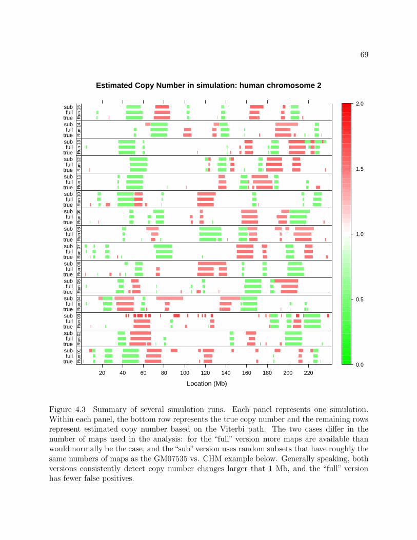
69

Estimated Copy Number in simulation: human chromosome 2

Location (Mb)

truefull

sub

20 40 60 80 100 120 140 160 180 200 220

Run

01

truefull

sub

Run

02

truefull

sub

Run

03

truefull

sub

Run

04

truefull

sub

Run

05

truefull

sub

Run

06

truefull

sub

Run

07

truefull

sub

Run

08

truefull

sub

Run

09

truefull

sub

Run

10

truefull

sub

Run

11

truefull

sub

Run

12

truefull

sub

Run

13

truefull

sub

Run

14

truefull

sub

Run

15

0.0

0.5

1.0

1.5

2.0

Figure 4.3 Summary of several simulation runs. Each panel represents one simulation.Within each panel, the bottom row represents the true copy number and the remaining rowsrepresent estimated copy number based on the Viterbi path. The two cases differ in thenumber of maps used in the analysis: for the “full” version more maps are available thanwould normally be the case, and the“sub”version uses random subsets that have roughly thesame numbers of maps as the GM07535 vs. CHM example below. Generally speaking, bothversions consistently detect copy number changes larger that 1 Mb, and the “full” versionhas fewer false positives.

70

States d.f. AIC BIC

1 2 9775.9 9786.7

2 5 9731.3 9758.1

3 10 9729.9 9783.5

Table 4.1 In comparing the GM07535 and CHM genomes, AIC and BIC values for HMMfits with 1, 2 and 3 states serve as a guide to choose the number of states. In this case, wechoose the model with 2 states.

optical maps represent a population that has 6 known sites each of decreased (1:2) and

elevated (3:2) copy number.

Figure 4.2 shows the results of fitting a 3-state negative binomial HMM to one such

data set. Figure 4.3 summarizes the results from multiple instances of this simulation. For

each simulation, models were fitted using the full data sets as well as smaller subsets. Copy

number changes larger that 1 Mb were detected more or less consistently, while smaller

regions were not. Surprisingly, the results obtained from the smaller data sets were not

much different, except in a couple of runs which had more false positives. Presumably, these

details will vary depending on the size of the genome and the number and magnitude of the

copy number alterations.

Example: GM07535 and CHM: We next considered optical map data from two hu-

man genomes, GM07535 and CHM (Section 1.2), restricting our attention to alignments to

the first 6 chromosomes. 23424 GM07535 and 43502 CHM optical maps aligned to these

chromosomes. Alignments of CHM maps were used as the normalizing genome to detect rel-

ative copy number changes in GM07535. Both genomes are believed to be “normal”, so not

much variation is expected. AIC and BIC values given in Table 4.1 provide some guidance

in selecting an appropriate number of states, and a model with 2 states seems appropriate.

Some regions of mild copy number differences are indicated by the graph of posterior prob-

abilities in Figure 4.4. The reason for the differences is not clear, but could in part reflect

heterozygous differences in GM07535.

71

Location (Mb)

Pos

terio

r pr

obab

ilitie

s

0.00.20.40.60.81.0

10 20 30 40 50 60 70 80 90 100 110 120 130 140 150 160 170 180 190 200 210 220 230

1

0.00.20.40.60.81.0

2

0.00.20.40.60.81.0

3

0.00.20.40.60.81.0

4

0.00.20.40.60.81.0

5

0.00.20.40.60.81.0

6

Figure 4.4 Coverage of the GM07535 genome normalized by CHM. Both are “normal”genomes, so we do not expect to see much variation. The HMM fit has two states, witha target normal state with 15 hits expected per interval. The estimated mean states areapproximately 11.66 and 16.31, with the higher state having a probability of 0.69 in thestationary distribution. Green bars represent posterior probabilities of the low state andgrey rectangles represent sequence gaps.

72

Example: MCF-7: A more interesting example is provided by the MCF-7 breast can-

cer cell line, which is known to exhibit copy number polymorphism (Pollack et al., 2002;

Volik et al., 2003). Figure 4.5 shows results for chromosomes 17 and 20, which have been

shown by other methods to contain short regions of strongly elevated copy number. 10540

MCF-7 optical maps align to these chromosomes. The combined alignments from GM07535

and CHM, totalling 7532, are used as the normalizing data set. For comparison, the figure

also shows data from the same cell line obtained using a completely different technology for

measuring array-based comparative genomic hybridization (CGH), namely the Affymetrix

Xba 50k chip (data provided by Prof. Paul Lizardi, Yale). A visual comparison shows that

the unsmoothed coverage counts track well with the raw CGH data. After smoothing using

the HMM for optical map data and the CBS algorithm (Olshen and Venkatraman, 2002) for

the Affymetrix data, the copy number estimates are also similar. Both methods detect the

short but prominent spikes in copy number.

4.4 Discussion

In this chapter, we have outlined an approach that uses optical map alignments to detect

copy number alterations in a genome. A key step in this process was to summarize alignments

of optical maps to an in silico reference by a single number (midpoint) representing location.

These locations were modeled as realizations of a non-homogeneous Poisson process. We

account for the non-homogeneity using alignment data from a normal genome, which are used

to define random intervals with counts that follow a negative binomial distribution. These

counts were then modeled by a Hidden Markov Model, incorporating spatial dependence in

the data and allowing more natural estimation of certain parameters.

Model building: In HMM’s, as in many other statistical techniques, model selection and

in particular the choice of the number of states, is more an art than a science. A small

number of states may not completely reflect reality, especially if the genome being studied is

a mixture, which would not be unusual in tumor samples. On the other hand, allowing many

73

(a) Observed counts and decoded (Viterbi) path

Location (mbp)

Cou

nts

4

8

16

32

64

128

10 20 30 40 50 60 70

17

4

8

16

32

64

128

20

Observed Decoded(b) Affymetrix XBA 50k chip

Location (mbp)lo

g2(m

ean)

− 1

0

2

4

0 20 40 60 80

17

0

2

4

20(c) Log (base 2) of Estimated Copy Number

Location (mbp)

Affymetrix

Optical maps

0 5 10 15 20 25 30 35 40 45 50 55 60 65 70 75 80

17

Affymetrix

Optical maps

20

−4

−3

−2

−1

0

1

2

3

4

Figure 4.5 Results for MCF-7 chromosomes 17 and 20. The grey curve in (a) plots (on alogarithmic scale) the number of MCF-7 alignments falling in intervals tiling each chromo-some. An HMM with 5 states is used to model this data, with emission probabilities givenby negative binomial distributions with a different mean for each state and a common sizeparameter. The parameters are estimated by the Baum-Welch algorithm using alignmentsto the two chromosomes, yielding an estimated size of 14.02 and estimated mean counts of12.43, 21.37, 27.28, 44.60 and 124.93. The black curve represents the most likely sequence ofunderlying states conditional on these parameters and the data. For comparison, (b) showsdata from the same cell line obtained using an Affymetrix Xba 50k chip, processed usingAffymetrix’ Copy Number Analysis Tool (CNAT). Estimated copy numbers are compareddirectly in (c), using the most likely (Viterbi) path for the HMM and the CBS algorithm forthe Affymetrix data.

74

states will usually lead to over-fitting: some estimated states may be close to each other and

rare states may not be identified at all. In practice, diagnostic plots and numerical criteria

like AIC and BIC may assist in making the choice. The estimated negative binomial size

parameter may also serve as a guide, since too few states in the model will be compensated

for by stronger apparent extra-Poisson variation. External information, when available, may

be used to put further constraints on the parameters, e.g. fixing the mean states up to a

multiplicative constant, which is estimated.

Normal state: The HMM does not assign the special label of“normality”to any particular

state. However, the initial choice of intervals are determined to have a specified mean number

of hits under the hypothesis of no copy number changes. In practice, the mean of the

stationary distribution of the estimated HMM is usually close to this initial choice. The

estimated mean state with the highest (stationary) probability is usually also the one closest

to this initial choice, and can be considered to be the normal state. This should work well

unless there is widespread CNP, in which case the definition of “normal state” is unclear.

Alignment: Alignment of optical maps to the in silico reference is an important pre-

requisite for our analysis. Although we expect and correct for non-uniform sensitivity, the

alignment scheme should nonetheless be as sensitive as possible with a low false positive rate.

In our examples, we have used the SOMA score function (A.1) with default parameters. The

determination of significance thresholds is discussed in Chapter 3. All alignments used were

significant at a nominal specificity of 99.9%.

Symmetry: High and low coverage are not treated symmetrically, in the sense that the

power to detect lowered coverage may be lower than that to detect elevated coverage of the

same relative magnitude. Thus, it may make sense to reverse the roles of the normal data

and the dataset of interest, so that low coverage is identified as high mean states in the

HMM. Of course, the relative sizes of the data sets are also relevant.

75

Conclusion: Copy number alterations are indicators of more complex structural variation.

While copy number information is useful in itself, especially for cancer genomes, it does not

tell the whole story. The promise of optical mapping is in its potential to discover a much

richer class of variation, including ones that are not clearly manifested as copy number

changes. Having said that, the methods described here are useful in identifying and locating

an important class of variation, and are often able to detect major events with relatively low

coverage. In all, the copy number analysis described here is a fast, simple tool that effectively

complements assembly-based analysis of optical map data.

76

Chapter 5

Future Work

In the previous chapters, we have described some recent contributions to the statistical

analysis of optical map data. In particular, we have addressed parameter estimation in

optical map models, the assessment of statistical significance of alignments, and the use of

optical map data to detect copy number alterations. Here, we briefly mention some possible

future directions of research that arise as natural extensions of the work reported here.

5.1 Alignment

Much of the recent success in the analysis of optical mapping data has revolved around

the alignment problem; specifically, alignment of optical maps against an in silico reference.

Not all questions concerning alignment have been answered yet, and we may expect more

successes by continuing research in this direction.

5.1.1 Score function

Principle: The conditional permutation test described in Chapter 3 is an important new

method that allows us to evaluate and compare different score functions. This gives us a tool

to experiment with new score functions and explore their suitability for various purposes.

Although we have primarily used the SOMA score in our analysis, its derivation is ad hoc

and somewhat unnatural from a probabilistic point of view. It can not be expressed in terms

of a likelihood ratio test, and parameters in the score often have no natural interpretation.

The model-based likelihood ratio score derived by Valouev et al. (2006) does not perform as

77

well in its current form, but their approach is fundamentally more sound and likely to give

better results in the long run with suitable modifications.

Purpose: Another consideration that should drive the choice of score function is the pur-

pose of alignment. Most existing score functions only attempt to account for mismatches

due to optical map noise. However, for the iterative assembly scheme described in Section

1.3.5, a score function will be more useful if it is designed to tolerate minor differences in

the underlying genome as well. Another situation where the choice of score function may be

important is local alignment. Separate local alignments of an optical map to different regions

of the reference may help identify translocations, in a manner similar to the end-sequence

profiling technique of Volik et al. (2003). In our investigations so far, the SOMA score has

not proven very useful for this purpose. As research continues, more situations are likely to

arise where new types of alignment scores will be required.

Software: Investigation of new score functions is currently somewhat hindered by the lack

of an easily extensible software platform to perform optical map alignment. Fortunately, the

SOMA software suite already implements the relevant algorithms and it should be relatively

simple to design a more powerful user interface around it.

5.1.2 Scale errors

Another possible enhancement to the current alignment scheme is to account for scaling

errors. Additive score functions used with dynamic programming assume that fragment

lengths are independent. However, as Figure 1.4 illustrates, the reported length of fragments

within a map may be scaled up or down together due to variability in estimating the scale

factor, causing the fragment lengths to be correlated. To explore this, recall notation from

Section 2.1.2 and consider the standardized errors

ǫi =Xi − µi√

σ2 (τ 2 + 1)µi + τ 2µ2i

78

Quantiles of Standard NormalO

bser

ved

Qua

ntile

s

−4

−2

0

2

4

−2 0 2

Raw errors

−2 0 2

Average errors

Figure 5.1 Correlation of sizing errors within map. The first panel is a normal Q-Q plot ofstandardized errors, using one randomly chosen ǫi for each map. The second panel is a Q-Qplot of the standardized mean errors ǫ. If within-map errors are uncorrelated, the ǫ’s andǫi’s should have the same variance. This is clearly not true.

(i = 1, . . . , n) for an optical map with n fragments. Each ǫi should have mean 0 and unit

variance. We can also define the standardized averages

ǫ =1√n

n∑

i=1

ǫi

If the ǫi’s are independent, ǫ should also have mean 0 and variance 1. If on the other hand

the errors within a map are positively correlated, then V (ǫ) > 1. This would be true if scale

errors are spatially correlated, i.e., nearby fragments are undersized or oversized together.

Using significant alignments of GM07535 optical maps, Figure 5.1 shows normal Q-Q plots

of the raw errors along with the standardized average errors ǫ, suggesting that within-map

sizing errors are indeed correlated.

Accounting for correlation: Additive scores assume independence of fragments and do

not allow for correlation, but it is still possible to indirectly account for it. One approach we

describe here is based on the premise that for an optical map with consistently undersized or

oversized fragments, the correct alignment will often be among the top scoring alignments

even if it does not exceed the threshold for significance. Assume that all fragments in a map

share a common estimated scale R. Given a potential alignment, one can estimate R; e.g.

if an alignment consists of pairs of aligned chunks (µi, Xi), i = 1, . . . , m, a possible estimate

is R =∑Xi/

∑µi. Other perhaps more robust estimates are also possible. The estimate

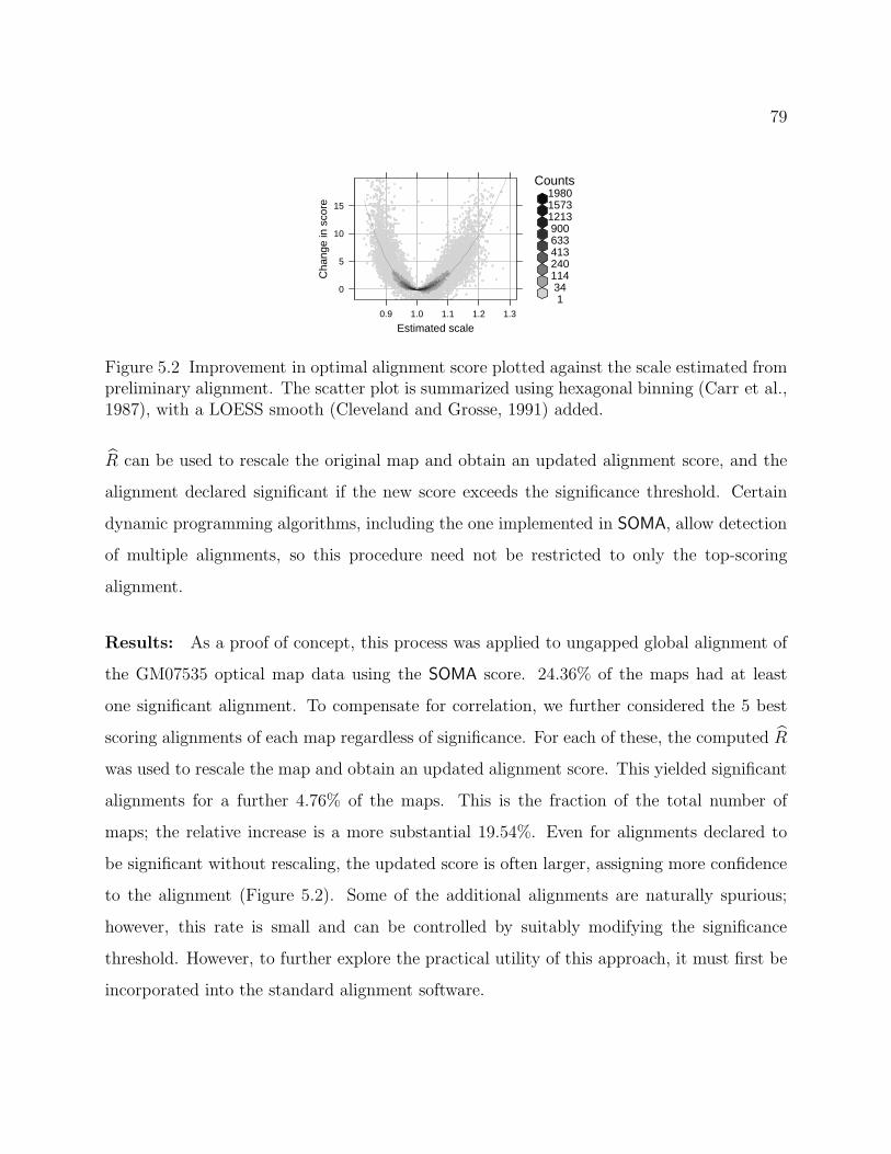
79

Estimated scaleC

hang

e in

sco

re

0

5

10

15

0.9 1.0 1.1 1.2 1.3

Counts

134

114240413633900

121315731980

Figure 5.2 Improvement in optimal alignment score plotted against the scale estimated frompreliminary alignment. The scatter plot is summarized using hexagonal binning (Carr et al.,1987), with a LOESS smooth (Cleveland and Grosse, 1991) added.

R can be used to rescale the original map and obtain an updated alignment score, and the

alignment declared significant if the new score exceeds the significance threshold. Certain

dynamic programming algorithms, including the one implemented in SOMA, allow detection

of multiple alignments, so this procedure need not be restricted to only the top-scoring

alignment.

Results: As a proof of concept, this process was applied to ungapped global alignment of

the GM07535 optical map data using the SOMA score. 24.36% of the maps had at least

one significant alignment. To compensate for correlation, we further considered the 5 best

scoring alignments of each map regardless of significance. For each of these, the computed R

was used to rescale the map and obtain an updated alignment score. This yielded significant

alignments for a further 4.76% of the maps. This is the fraction of the total number of

maps; the relative increase is a more substantial 19.54%. Even for alignments declared to

be significant without rescaling, the updated score is often larger, assigning more confidence

to the alignment (Figure 5.2). Some of the additional alignments are naturally spurious;

however, this rate is small and can be controlled by suitably modifying the significance

threshold. However, to further explore the practical utility of this approach, it must first be

incorporated into the standard alignment software.

80

5.2 Other topics

Preliminary filtering: The optical mapping pipeline processes massive amounts of data.

This process is helped if maps that are unlikely to contribute to the results are filtered

out beforehand. It is currently standard practice to leave out maps that do not exceed a

minimum length threshold, usually 300 Kb. However, length of an optical map does not

by itself determine the usefulness of a map. As suggested in Section 3.4.2, one alternative

is to use a map-specific information score, derived from alignment score functions, for this

purpose. A similar but more difficult line of research would be to develop a map-specific

confidence score as part of the image processing step, to reflect the likely quality of the map.

Iterative assembly: The iterative assembly scheme described by Reslewic et al. has been

successful in assembling large genomes by taking advantage of an initial reference map. Being

a first attempt, there is naturally scope for improvement. Although the results have been

validated to some extent (e.g. using PCR), the use of Gentig as an assembly tool must

be regarded as heuristic, since the set of input maps is highly selective and not random

as the model expects. Further, the depth of these data sets are lower than the values

suggested by Anantharaman and Mishra (2003) for reliable assemblies, which may explain

alignment problems involving small fragments. Generally speaking, the inherent trade-off

between depth (resources) and accuracy is unavoidable, and low depth may be an acceptable

compromise in many situations. However, a formal study is necessary to quantify this trade-

off. Also desirable are formal approaches to develop rules to control false positives, which

are currently derived in an ad hoc fashion. One specific goal is to obtain an estimate for the

false positive rate, which is not obvious even in the case where the true genome is known.

General questions: More generally, several algorithmic questions remain unanswered.

The most obvious one is de novo assembly for large genomes, which is required when a draft

sequence is not available. Another consideration is the analysis of heterozygous or mixture

(e.g. cancer) populations. This is particularly important in studying human genomes, which

81

will rarely be homozygous. It may also be beneficial to consider fresh approaches when

dealing with genomes that have a reliable sequence. While minor variations can be detected

by the assembly scheme described above, it is unclear how well it would do for larger events

such as translocations and rearrangements. It is entirely possible that a full assembly is

unnecessary to detect such variations, and more direct strategies exist that take advantage

of the in silico reference.

82

LIST OF REFERENCES

S. F. Altschul. Amino acid substitution matrices from an information theoretic perspective.Journal of Molecular Biology, 219:555–565, 1991.

T. S. Anantharaman and B. Mishra. Genomics via Optical Mapping. I: 0-1 Laws for SingleMolecules. Technical report, New York University, 2003.

T. S. Anantharaman, B. Mishra, and D. C. Schwartz. Genomics via Optical Mapping. II:Ordered Restriction Maps. Journal of Computational Biology, 4:91–118, 1997.

T. S. Anantharaman, B. Mishra, and D. C. Schwartz. Genomics via Optical Mapping. III:Contiging Genomic DNA. In Proc Int Conf Intell Syst Mol Biol., pages 18–27, 1999.

E.V. Armbrust, J.A. Berges, C. Bowler, B.R. Green, D. Martinez, N.H. Putnam, S. Zhou,A.E. Allen, K.E. Apt, M. Bechner, M.A. Brzezinski, B.K. Chaal, A. Chiovitti, DavisAK, M.S. Demarest, J.C. Detter, T. Glavina, D. Goodstein, M.Z. Hadi, U. Hellsten,Hildebrand M, B.D. Jenkins, J. Jurka, V.V. Kapitonov, N. Kroger, W.W. Lau, T.W.Lane, Larimer FW, J.C. Lippmeier, S. Lucas, M. Medina, A. Montsant, M. Obornik,M.S. Parker, B. Palenik, G.J. Pazour, Richardson PM, T.A. Rynearson, M.A. Saito, D.C.Schwartz, Thamatrakoln K, K. Valentin, A. Vardi, F.P. Wilkerson, and D.S. Rokhsar.The genome of the diatom thalassiosira pseudonana: ecology, evolution, and metabolism.Science, 306(5693):79–86, Oct 1 2004.

L.E. Baum. An inequality and associated maximization technique in statistical estimationof Markov processes. Inequalities, 3:1–8, 1972.

D. B. Carr et al. Scatterplot matrix techniques for large n. JASA, 83:424–436, 1987.

William S. Cleveland and E. Grosse. Computational methods for local regression. Statisticsand Computing, 1:47–62, 1991.

International Human Genome Sequencing Consortium. Finishing the euchromatic sequenceof the human genome. Nature, 431(7011):931–945, Oct 21 2004.

D. R. Cox and D. V. Hinkley. Theoretical Statistics. Chapman & Hall Ltd, 1979.

83

E.T. Dimalanta, A. Lim, R. Runnheim, C. Lamers, C. Churas, D.K. Forrest, J.J. dePablo,M.D. Graham, S.N. Coppersmith, and D.C. Schwartz. A microfluidic system for large dnamolecule arrays. Anal. Chem., 76:5293–5301, 2004.

R. Durbin, S. Eddy, A. Krogh, and G. Mitchison. Biological Sequence Analysis: ProbabilisticModels of Proteins and Nucleic Acids. Cambridge University Press, 1998.

Evan E. Eichler. Widening the spectrum of human genetic variation. Nature Genetics, 38:9–11, 2006.

J.B. Fan, U. Surti, P. Taillon-Miller, L. Hsie, G.C. Kennedy, L. Hoffner, T. Ryder, D.G.Mutch, and P.Y. Kwok. Paternal origins of complete hydatidiform moles proven by wholegenome single-nucleotide polymorphism haplotyping. Genomics, 79(1):58–62, January2002.

E. J. Gumbel. Sommes et differences de valeurs extremes independentes. Comptes Rendusde l’Academie des Sciences, Paris, 253:2838–2839, 1961.

Xiaoqiu Huang and Michael S. Waterman. Dynamic programming algorithms for restrictionmap comparison. CABIOS, 8(5):511–520, 1992.

A.C. Ivens, C.S. Peacock, E.A. Worthey, L. Murphy, G. Aggarwal, M. Berriman, E. Sisk,M.A. Rajandream, E. Adlem, R. Aert, A. Anupama, Z. Apostolou, P. Attipoe, N. Bason,C. Bauser, A. Beck, S.M. Beverley, G. Bianchettin, Borzym K, G. Bothe, C.V. Bruschi,M. Collins, E. Cadag, Ciarloni L, C. Clayton, R.M. Coulson, A. Cronin, A.K. Cruz,Davies R.M., J. De Gaudenzi, D.E. Dobson, A. Duesterhoeft, G. Fazelina, N. Fosker, A.C.Frasch, A. Fraser, M. Fuchs, C. Gabel, A. Goble, A. Goffeau, D. Harris, C. Hertz-Fowler,H. Hilbert, D. Horn, Y. Huang, S. Klages, A. Knights, M. Kube, N. Larke, L. Litvin,A. Lord, T. Louie, M. Marra, D. Masuy, K. Matthews, S. Michaeli, J.C. Mottram,S. Muller-Auer, H. Munden, S. Nelson, H. Norbertczak, K. Oliver, S. O’neil, M. Pentony,T.M. Pohl, C. Price, B. Purnelle, M.A. Quail, E. Rabbinowitsch, R. Reinhardt, M. Rieger,J. Rinta, J. Robben, L. Robertson, J.C. Ruiz, S. Rutter, D. Saunders, M. Schafer, J. Schein,D.C. Schwartz, K. Seeger, A. Seyler, S. Sharp, H. Shin, D. Sivam, R. Squares, S. Squares,V. Tosato, C. Vogt, G. Volckaert, R. Wambutt, T. Warren, H. Wedler, J. Woodward,S. Zhou, W. Zimmermann, D.F. Smith, J.M. Blackwell, K.D. Stuart, B. Barrell, and P.J.Myler. The genome of the kinetoplastid parasite, Leishmania major. Science, 309(5733):436–442, July 15 2005.

Scott Kohn. Software for Optical Map Analyis, 2003. SOMA.

E. S. Lander and M. S. Waterman. Genomic mapping by fingerprinting random clones: amathematical analysis. Genomics, 2:231–239, 1988.

Michael A. Newton. Discovering combinations of Genomic aberrations associated with can-cer. Journal of the American Statistical Association, 97(460):931–942, 2002.

84

A. Olshen and E. Venkatraman. Change-point analysis of array-based comparative genomichybridization data. Proc. of Joint Statistical Meetings, pages 2530–2535, 2002.

J.R. Pollack, T. Sorlie, C. Perou, C. Rees, S. Jeffrey, P. Lonning, R. Tibshirani, D. Botstein,A. Borresen-Dale, and P. Brown. Microarray analysis reveals a major direct role of DNAcopy number alteration in the transcriptioanl program of human breast tumors. Proc.Natl. Acad. Sci. USA, 99:12963–12968, 2002.

Susan Reslewic, Alex Lim, Anton Valouev, Steve Goldstein, Chris Churas, Michael S. Wa-terman, Lei Li, Scott Kohn, Deepayan Sarkar, Marijo Kent-First, Dan Forrest, RodRunnheim, Michael A. Newton, Urvashi Surti, Miron Livny, and David C. Schwartz. TheHuman Genome Analyzed by Single DNA Molecules.

D. C. Schwartz, X. Li, L.I. Hernandez, S.P. Ramnarain, E.J. Huff, and Y.K. Wang. Or-dered restriction maps of Saccharomyces cerevisiae chromosomes constructed by opticalmapping. Science, 262:110–114, 1993.

J. Setubal and J. Meidanis. Introduction to Computational Molecular Biology. PWS Pub-lishing Company, 1997.

Anton Valouev, Lei Li, Yu-Chi Liu, David C. Schwartz, Yi Yang, Zhang Yu, and Michael S.Waterman. Alignment of Optical Maps. Journal of Computational Biology, 13(2):442–462,2006.

A.W. van der Vaart. Asymptotic Statistics. Cambridge University Press, 1998.

S. Volik, S. Zhao, K. Chin, J.H. Brebner, D.R. Herndon, Q. Tao, D. Kowbel, G. Huang,A. Lapuk, W.L. Kuo, G. Magrane, P. De Jong, J.W. Gray, and C. Collins. End-sequenceprofiling: sequence-based analysis of aberrant genomes. Proc. Natl. Acad. Sci. USA, 100:7696–7701, 2003.

M. S. Waterman, T. F. Smith, and H. L. Katcher. Algorithms for restriction map comparison.Nucleic Acid Res, 12:237–242, 1984.

Michael S. Waterman. Introduction to Computational Biology: Maps, Sequences andGenomes. Chapman and Hall/CRC, 1995.

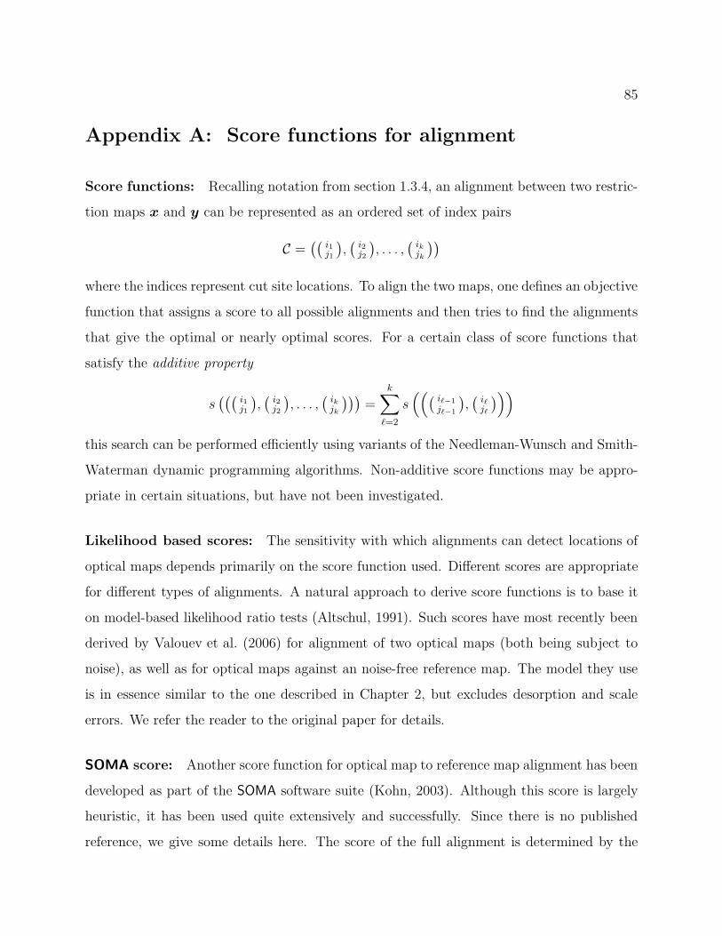
85

Appendix A: Score functions for alignment

Score functions: Recalling notation from section 1.3.4, an alignment between two restric-

tion maps x and y can be represented as an ordered set of index pairs

C =((

i1j1

),(i2j2

), . . . ,

(ikjk

))

where the indices represent cut site locations. To align the two maps, one defines an objective

function that assigns a score to all possible alignments and then tries to find the alignments

that give the optimal or nearly optimal scores. For a certain class of score functions that

satisfy the additive property

s(((

i1j1

),(i2j2

), . . . ,

(ikjk

)))=

k∑

ℓ=2

s((( iℓ−1

jℓ−1

),(iℓjℓ

)))

this search can be performed efficiently using variants of the Needleman-Wunsch and Smith-

Waterman dynamic programming algorithms. Non-additive score functions may be appro-

priate in certain situations, but have not been investigated.

Likelihood based scores: The sensitivity with which alignments can detect locations of

optical maps depends primarily on the score function used. Different scores are appropriate

for different types of alignments. A natural approach to derive score functions is to base it

on model-based likelihood ratio tests (Altschul, 1991). Such scores have most recently been

derived by Valouev et al. (2006) for alignment of two optical maps (both being subject to

noise), as well as for optical maps against an noise-free reference map. The model they use

is in essence similar to the one described in Chapter 2, but excludes desorption and scale

errors. We refer the reader to the original paper for details.

SOMA score: Another score function for optical map to reference map alignment has been

developed as part of the SOMA software suite (Kohn, 2003). Although this score is largely

heuristic, it has been used quite extensively and successfully. Since there is no published

reference, we give some details here. The score of the full alignment is determined by the

86

score of each chunk(( iℓ−1

jℓ−1

),(iℓjℓ

)). Let ν be the length of the reference map in the chunk,

and x be the corresponding optical map length. Further, let m = iℓ − iℓ−1 be the number

of reference map fragments combined to form length ν, and n = jℓ − jℓ−1 be the number of

optical map fragments combined to form length x (thus, u = m− 1 is the number of missing

cut sites and v = n− 1 the number of false cut sites). Then, the contribution of this chunk

to the final score is given by

s(ν, x,m, n) = log

(1 +

ν + x

2λ

)×

(1 − (x− ν)2

C(ν)− uPm − vPf

) (A.1)

where Pm is a missing cut penalty, Pf is a false cut penalty, C(ν) is a sizing error cutoff

(related to the variance of the sizing errors) and λ represents the mean reference fragment

length. The log term is intended to give higher weight to longer fragments. A critical

component of the score is the choice of C(ν); empirically, a form piecewise linear in ν2 has

been found to be useful. This is consistent with the marginal sizing variance derived in

Chapter 2, and can be viewed as an approximation to the latter, more recent, form. A

further adjustment intended to correct for desorption is used as follows: instead of counting

each missing cut site as one to give a total of u = m − 1, each missing cut contributes the

quantity π(y), the probability of retaining a fragment of size y, where y is the distance from

the missing cut site to the nearest observed cut site. Unlike the likelihood ratio based scores,

there is no natural interpretation for the score of the complete alignment, which is simply

the sum of the scores for individual aligned chunks.

87

Appendix B: Hidden Markov Model calculations

Negative binomial emissions: Since our analysis is based on interval counts of events

modeled by a Poisson point process, it is natural to model the counts by a Poisson distribu-

tion. Due to inhomogeneity of the process, the distribution of the counts are not determined

solely by the interval lengths. To normalize the counts, we choose data dependent inter-

vals, thus altering the count distribution. With this modification, the counts are no longer

Poisson, but negative binomial, a fact which follows from the following

Lemma 1. Let X1 < · · · < Xm be observed event times from a (possibly non-homogeneous)

Poisson process with rate λ(·) and Y1 < · · · < Yn be observed event times from a Poisson

process with rate αλ(·). Let G = (Xℓ, Xℓ+p+1] for some ℓ ∈ {1, . . . , m− p− 1} and N =∑

k I{Yk∈G}. Then, N has a negative binomial distribution with mean αp and size p.

Proof. Without loss of generality, assume that both processes are homogeneous; if not, they

can be homogenized by a transformation of the time axis determined by λ(·). Also assume

w.l.g. that λ(t) = 1 ∀t, in which case the (Yk)n

1 process has constant intensity α. Then,

the length of G, denoted |G|, is the waiting time till the pth event of a homogeneous Poisson

process with unit intensity, or equivalently, the sum of p independent standard exponentials.

Thus, |G| has the Gamma distribution with shape parameter p, and N |G ∼ Poisson (α|G|)by definition. The proof is completed by noting that the negative binomial distribution can

be expressed as a Gamma mixture of Poissons, with parameters as specified in the lemma.

We use a somewhat non-standard parameterization of the negative binomial distribution,

where the mass function of a random variable X with mean µ and size σ, denoted X ∼NB (µ, σ), is given by

p(X = x) =Γ(x+ σ)

Γ(σ) x!

(σ

σ + µ

)σ (µ

σ + µ

)x

This has the nice property that E(X) = µ and V (X) = µ + µ2

σ. The distribution of X

converges in distribution to Poisson (µ) as σ → ∞. In practice, the size parameter may

account for lack of fit in the model as well.

88

Baum-Welch updates: The parameter estimation step of the HMM needs some calcu-

lations specific to the negative binomial model. To state the results, we first need some

notation, which roughly follows Durbin et al. (1998). The data is assumed to be a sequence

(xi)L

i=1 of observed hits in L successive intervals along the genome, with the corresponding

sequence of random variables being denoted by (Xi)L

i=1. In practice, the data will be in

the form of several sequences (e.g. one for every chromosome). The derivations done below

generalize trivially to this situation, provided we assume that all the sequences are generated

by the same model. Each observation Xi has an associated hidden state Πi. We will often

abbreviate (xi)L

i=1 by x, (Xi)L

i=1 by X and (Πi)L

i=1 by Π. The unobserved sequence (Πi)L

i=1 is

a time-homogeneous stationary Markov process with a finite state space S = {1, 2, . . . , K}.The distribution of Xi is entirely determined by Πi. This distribution is defined by the

emission probabilities

ek(b) = P (Xi = b|Πi = k) (B.1)

The evolution of the process (Πi)L

i=1 is governed by the transition probability matrix P,

which has entries

ak,l = P (Πi+1 = l|Πi = k) (B.2)

and stationary distribution π0. The parameters in the model consist of the transition prob-

abilities a = ((ak,l)) along with any parameters involved in the emission distribution, which

we denote by η. Collectively, the parameters are denoted by θ = (a,η). Estimation of the

parameters, often referred to as ‘training’, can be accomplished by using the Baum-Welch

algorithm, which can also be stated in terms of the more familiar EM algorithm. It is an

iterative procedure generally described in terms of observed data, missing data and param-

eters. In our case, the observed data are x and the missing data are the hidden states Π.

Given a current estimate for θ, say θt, the E-step involves computing the function

Q(θ|θt) =∑

Π

P(Π|X = x, θt

)log P (X = x,Π|θ) (B.3)

and the M-step involves obtaining the next iterate

θt+1 = arg maxθ

Q(θ|θt) (B.4)

89

which can be shown to have higher likelihood than θt.

The details of these calculations depend on the emission model. We consider two specific

models for the emission distribution (B.1). In the first model, η = (λ1, . . . , λK , σ), which

defines the emission distributions

Xi|Πi = k ∼ NB (λk, σ) (B.5)

In words, the emission distribution in each state is negative binomial with a different mean

and a common size parameter. The second model attempts to ensure that copy number

changes are limited to simple fractions (e.g. 2:3, 1:2, 1:1, 2:1, 3:2) by fixing them relative to

each other. Specifically, η = (λ, σ) and

Xi|Πi = k ∼ NB (λαk, σ) (B.6)

where α1, . . . , αK are fixed known constants. Theorem 1 gives the Baum-Welch updates for

these two models in terms of the quantities

Ak,l =

L−1∑

i=1

I{Πi=k,Πi+1=l}

Bk =L−1∑

i=1

I{Πi=k}

Nk,b =

L−1∑

i=1

I{Πi=k,xi=b}

and

Ak,l(θ) = E (Ak,l|x, θ)

Bk(θ) = E (Bk|x, θ)

Nk,b(θ) = E (Nk,b|x, θ)

The proof of the theorem is long but straightforward, and will not be given here.

90

Theorem 1. For model (B.5), where θ consists of ((ak,l)), λk and σ,

Q(θ|θt) =

K∑

k=1

K∑

l=1

Ak,l(θ) log ak,l

+∑

i

log Γ(xi + σ) − (L− 1) log Γ(σ)

−∑

i

log xi! + σ

K∑

k=1

Bk(θ) log

(σ

σ + λk

)

+∞∑

b=0

K∑

k=1

Nk,b(θ) b log

(λk

σ + λk

)

The updates for a and η are given by

at+1k,l =

Ak,l(θ)∑K

l=1 Ak,l(θ), 1 ≤ k, l ≤ K (B.7)

λt+1k =

∑∞b=0 b Nk,b(θ)

Bk(θ), 1 ≤ k ≤ K (B.8)

σt+1 has no closed form solution, but can be obtained by numerically solving a one dimen-

sional optimization problem after substituting (B.7) and (B.8) in Q(θ|θt). (B.7) and (B.8)

also hold in the limiting case, as σ → ∞, when the emission distribution can be approximated

by a Poisson distribution. For model (B.6),

Q(θ|θt) =

K∑

k=1

K∑

l=1

Ak,l log ak,l

+∑

i

log Γ(xi + σ) − (L− 1) log Γ(σ)

−∑

i

log xi! + σ

K∑

k=1

Bk log

(σ

σ + λαk

)

+∞∑

b=0

K∑

k=1

Nk,b b log

(λαk

σ + λαk

)

In this case neither σt+1 nor λt+1 have a closed form solution, and both have to be obtained

numerically. For the limiting Poisson model, λt+1 is given by

λt+1 =

∑i xi∑K

k=1 Bkαk(B.9)