On the all-pairs shortest-path algorithm of Moffat and Takaoka

} }< <

On the All-Pairs Shortest-Path Algorithmof Moffat and Takaoka*

Kurt Mehlhorn, Volker PriebeMax-Planck-Institut fur Informatik, Im Stadtwald, 66123 Saarbrucken, Germany¨ ¨

Recei ed 20 December 1995; reïsed 25 August 1996

ABSTRACT: We review how to solve the all-pairs shortest-path problem in a nonnegativelyŽ 2 .weighted digraph with n vertices in expected time O n log n . This bound is shown to hold

with high probability for a wide class of probability distributions on nonnegatively weightedŽ .digraphs. We also prove that, for a large class of probability distributions, V n log n time is

necessary with high probability to compute shortest-path distances with respect to a singleŽ .source. Q 1997 John Wiley & Sons, Inc. Random Struct. Alg., 10, 205]220 1997

Key Words: shortest-path problems; probabilistic analysis; tail estimates; lower bound

1. INTRODUCTION

Given a complete digraph in which all the edges have nonnegative length, we wantto compute the shortest-path distance between each pair of vertices. This is one ofthe most basic questions in graph algorithms, since a variety of combinatorial-opti-mization problems can be expressed in these terms. As far as worst-case complexity

Ž 3.is concerned, we can solve an n-vertex problem in time O n either by Floyd’sw x w x w xalgorithm 4 or by n calls of Dijkstra’s algorithm 2 . Fredman’s algorithm 5 uses

*A preliminary version of this paper was presented at the Third Annual European Symposium onw xAlgorithms, Corfu, Greece, 1995 12 .

Correspondence to: V. PriebeQ 1997 John Wiley & Sons, Inc. CCC 1042-9832r97r100205-16

205

MEHLHORN AND PRIEBE206

efficient distance-matrix multiplication techniques and results in a running time ofŽ 3ŽŽ . .1r3. Ž Ž 3ŽŽ . .1r2 .O n log log n rlog n slightly improved to O n log log n rlog n by

w x. w xTakaoka 17 . Recently, Karger, Koller, and Phillips 10 presented an algorithmŽ U 2 . Uthat runs in time O nm qn log n , where m denotes the number of edges that

are a shortest path from their source to their target.However, worst-case analysis sometimes fails to bring out the advantages of

algorithms that perform well in practice; average-case analysis has turned out to bemore appropriate for these purposes. We are not only interested in algorithms withgood expected running time but in algorithms that finish their computations within

Ž .a certain time bound with high probability and might therefore be called reliable .Two kinds of probability distributions on nonnegatively weighted complete

digraphs have been considered in the literature. In the so-called uniform model, theedge weights are independent, identically distributed random variables. In the

Ž .so-called endpoint-independent model, an arbitrary multi- set c , 1F jFn, of n¨ j

Ž .nonnegative weights possibly ` is fixed for each vertex ¨ . These weights areassigned randomly to the n edges with source ¨ , i.e., a random bijective mapping

Ž¨ . � 4p from 1, . . . , n to V is chosen and c is made the weight of the edge¨ jŽ Ž¨ .Ž ..¨ , p j for all j, 1F jFn.

w x Ž 2 .Frieze and Grimmett 7 gave an algorithm with O n log n expected runningtime in the uniform model when the common distribution function F of the edge

Ž . XŽ . XŽ .weights satisfies F 0 s0, F 0 exists, and F 0 )0. Under these assumptions,U Ž . w xm sO n log n with high probability, and so the algorithm of Karger et al. 10

Ž 2 .also achieves running time O n log n with high probability.The endpoint-independent model is more general and harder to analyze. Spira

w x Ž 2Ž .2 .16 proved an expected time bound of O n log n , which was later improved byw x Ž 2 . ŽBloniarz 1 to O n log n log* n . We use log to denote logarithms to base 2 and

ln to denote natural logarithms; logU x[1 for xF2 and logU x[1q logU log x for. w x w xx)2. In 13 and 14 , Moffat and Takaoka describe two algorithms with an

Ž 2 . w xexpected time bound of O n log n . The algorithm in 14 is a simplified version ofw x w xthat of 13 . In Section 3 of this paper, we review the algorithm in 14 and the

analysis of its expected running time. We point out some easy-to-make mistakes inthe analysis and show how to avoid them. Moreover, we prove that the running

Ž 2 .time of the algorithm is O n log n with high probability. In Section 4, we showŽ .that under modest assumptions V n log n edges need to be inspected to compute

the shortest-path distances with respect to a single source.

2. PRELIMINARIES

We will refer to the following probabilistic experiments. Let an urn contain n ballsthat are either red or blue; let r be the number of red balls. The balls are

Ž .repeatedly drawn from the urn without replacement uniformly at random. Let Wbe the number of drawings until the first red ball occurs; then

ny r n nyk nw xE W s Pr W)k s s ,Ž .Ý Ý Ý ž / ž /ž / ž / r rk k0FkFnyr 0FkFnyr 0FkFnyr

ALL-PAIRS SHORTEST-PATH ALGORITHM 207

nq 1 y k n y kn y kand from s y , we conclude thatž / ž / ž /r rq 1 r q 1

nq1nq1 nw xE W s s .ž /ž / rrq1 rq1

We are also interested in sampling with replacement. Suppose that in a sequenceof independent trials, the probability of success is p for each of the trials. Let Z bethe number of trials until the first successful one; then

kw xE Z s Pr Z)k s 1yp s1rp.Ž . Ž .Ý ÝkG0 kG0

In the so-called coupon-collector problem, we are given a set of n distinct couponsand we are trying to complete a collection of all coupons. In each trial, a coupon is

Ž .drawn with replacement uniformly and independently at random. We call a trial asuccess if it results in adding a new coupon to our collection. Let ZU denote thecompletion time, i.e., the number of trials required to have seen at least one copyof each coupon. ZU s1qZ q ??? qZ , where for 1F i-n, Z is the number of1 ny1 i

ny iŽ . Ž .trials with probability of success each between the ith and iq1 th successnnŽ . w xexcluding the former, including the latter . By the argument above, E Z s ,i ny i

U nw x Ž . Ž .and hence, E Z sÝ Fn ln nq1 sO n ln n .0 F i- n ny i

For a problem of size n, we will say that an event occurs with high probability if itŽ yC .occurs with probability G1yO n for an arbitrary but fixed constant C. For

Ž .example, in the coupon-collector problem with n coupons , the probability that a1 tŽ .particular coupon has not been collected after t trials equals 1y . Hence, forn

any b)1,

b n ln n1U yb ln n yŽ by1.Pr Z )b n ln n Fn 1y Fne sn ; 1Ž . Ž .ž /n

Ž .that is, the completion time in the coupon-collector problem with n coupons isŽ . Ž .O n ln n with high probability. 1 establishes what is called a large-de iation

U Ž U .estimate for Z , i.e., a bound on Pr Z )z , where z is of about the order ofw U xE Z .

We are actually interested in a large-deviation estimate for a random variableX U [1qX q ??? qX , where each X is stochastically dominated by the ran-1 ny1 idom variable Z from the coupon-collector problem. For two random variables Xiand Y taking values in the positive integers, X is said to be stochastically dominated

Ž . Ž .by Y, written XF Y, if Pr X)k FPr Y)k for all kG0. Note that XF Yst stw x w ximplies E X FE Y . Stochastic dominance is preserved under taking sums of

independent random variables, i.e., if X , . . . , X , Y , . . . , Y are independent and1 n 1 nw xX F Y for 1F iFn, then X q ??? qX F Y q ??? qY ; see, for example, 18 .i s t i 1 n st 1 n

We will need the following, slightly more general result, which is a generalizationw xof Lemma 7 of 15 .

Lemma 1. Let X , . . . , X , Y , . . . , Y be random äriables that take älues in the1 n 1 npositi e integers. Suppose that each X , 1F iFn, conditioned on any possible tuple ofiälues for X , . . . , X , is stochastically dominated by Y , and that Y , . . . , Y are1 iy1 i 1 nindependent. Then X Žn.[Ý X is stochastically dominated by Y Žn.[Ý Y .1F iF n i 1F iF n i


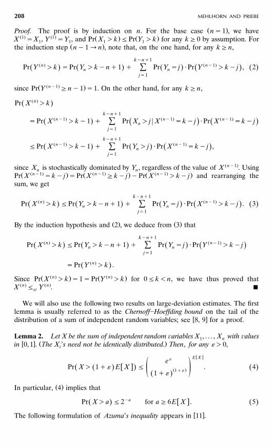
Ž .Proof. The proof is by induction on n. For the base case ns1 , we haveŽ1. Ž1. Ž . Ž .X sX , Y sY , and Pr X )k FPr Y )k for any kG0 by assumption. For1 1 1 1

Ž .the induction step ny1ªn , note that, on the one hand, for any kGn,

kynq1Žn. Žny1.Pr Y )k sPr Y )kynq1 q Pr Y s j ?Pr Y )ky j , 2Ž . Ž . Ž . Ž .Ž .Ýn n

js1

Ž Žny1. .since Pr Y Gny1 s1. On the other hand, for any kGn,

Pr X Žn.)kŽ .kynq1

Žny1. Žny1. Žny1.sPr X )ky1 q Pr X ) j ¬ X sky j ?Pr X sky jŽ . Ž .Ž .Ý njs1

kynq1Žny1. Žny1.FPr X )ky1 q Pr Y ) j ?Pr X sky j ,Ž . Ž . Ž .Ý n

js1

since X is stochastically dominated by Y , regardless of the value of X Žny1.. Usingn nŽ Žny1. . Ž Žny1. . Ž Žny1. .Pr X sky j sPr X Gky j yPr X )ky j and rearranging the

sum, we get

kynq1Žn. Žny1.Pr X )k FPr Y )kynq1 q Pr Y s j ?Pr X )ky j . 3Ž . Ž . Ž . Ž .Ž .Ýn n

js1

Ž . Ž .By the induction hypothesis and 2 , we deduce from 3 that

kynq1Žn. Žny1.Pr X )k FPr Y )kynq1 q Pr Y s j ?Pr Y )ky jŽ . Ž . Ž . Ž .Ýn n

js1

sPr Y Žn.)k .Ž .

Ž Žn. . Ž Žn. .Since Pr X )k s1sPr Y )k for 0Fk-n, we have thus proved thatX Žn.F Y Žn.. Bst

We will also use the following two results on large-deviation estimates. The firstlemma is usually referred to as the Chernoff]Hoeffding bound on the tail of the

w xdistribution of a sum of independent random variables; see 8, 9 for a proof.

Lemma 2. Let X be the sum of independent random äriables X , . . . , X with älues1 nw x Ž .in 0, 1 . The X ’s need not be identically distributed. Then, for any «)0,i

w xE X«ew xPr X) 1q« E X F . 4Ž . Ž .Ž . Ž .1q«ž /1q«Ž .

Ž .In particular, 4 implies that

ya w xPr X)a F2 for aG6E X . 5Ž . Ž .

w xThe following formulation of Azuma’s inequality appears in 11 .


Lemma 3. Let X , . . . , X be independent random äriables, with X taking älues in1 n k< Ž . Ž . <a set A for each k. Suppose that the function f :Ł A ªR satisfies f x y f y Fck k

wheneër the ëctors x and y differ only in a single coordinate. Let Y be the randomŽ .äriable f X , . . . , X . Then, for any t)0,1 n

< < y2 t 2 rŽ nc2 .w xPr YyE Y G t F2 e .Ž .

3. THE ALGORITHM OF MOFFAT AND TAKAOKA

Ž .We use the following terminology for weighted digraphs. For an edge es ¨ , w , wecall ¨ the source and w the target or endpoint of e. The weight of an edge e is

Ž .denoted by c e . We will interpret an entry in the adjacency list of a vertex ¨ eitherŽ .as the endpoint w of an edge with source ¨ or as the edge ¨ , w itself, as is

convenient.For the sake of future reference, we briefly review the algorithm of Moffat and

w x Ž .Takaoka in 14 . We are given a complete digraph with loops on n vertices withnonnegative edge weights. The algorithm first sorts all adjacency lists in order of

Ž Ž 2 ..increasing weight with ties resolved randomly, total time O n log n and thensolves n single-source shortest-path problems, one for each vertex. A single-sourceshortest-path problem with source sgV is solved by labeling the vertices in orderof increasing distance from the source. If ¨ is a labeled vertex, then its exact

Ž .distance d ¨ from the source is known. We use S to denote the set of labeledvertices and UsVyS to denote the set of unlabeled vertices. Initially, only the

� 4 Ž .source vertex is labeled, i.e., Ss s with d s s0. For each labeled vertex ¨ , oneŽ .of its outgoing edges is called its current edge and is denoted ce ¨ ; we maintain the

Ž .invariant that all edges preceding the current edge ce ¨ in ¨ ’s adjacency list haveŽ . Žtheir endpoints already labeled. We say that the edges preceding ce ¨ as well as

.their targets have been scanned by the algorithm. The potential of ¨ ’s currentŽ . Ž Ž ..edge is defined as d ¨ qc ce ¨ . The algorithm proceeds in iterations. In each

iteration, the algorithm selects the current edge of minimum potential; supposeŽ .that ce ¨ is selected and that w is its target. If w is not yet labeled, then the

Ž . Ž . Ž . Ž Ž .. Žalgorithm labels w i.e., adds w to S and sets d w to d ¨ qc ce ¨ . It followsŽ .by a standard argument as for Dijkstra’s algorithm that this indeed sets d w to the

.distance of w from s. Moreover, some current-edge pointers are updated. Theprecise nature of these updates depends on the size of U.

< <As long as U )nrlog n, the algorithm is said to be in Phase I, and theadditional invariant is maintained that the targets of all current edges are unla-

Ž .beled. Whenever the algorithm selects a current edge ce ¨ of minimum potential,Ž .the target of ce ¨ will therefore be a vertex u in U. The algorithm labels u and

Ž . Ž . Ž Ž ..sets d u to d ¨ qc ce ¨ . In order to maintain the invariant of Phase I, thealgorithm advances the current-edge pointer of u and the current-edge pointers ofall the vertices whose current edges end in u; the pointers are advanced to the next

< <edge with target in VyS in the respective adjacency lists. Phase I ends when Ubecomes nrlog n; let U be the set of unlabeled vertices at the end of Phase I.0


< <If U Fnrlog n, the algorithm is said to be in Phase II, and the weakeradditional invariant is maintained that the endpoint of every current edge belongs

Ž . Ž .to U . Suppose that the current edge ce ¨ s ¨ , w is selected in an iteration. The0vertex wgU is not necessarily unlabeled. If w is unlabeled, it will be labeled,0Ž . Ž . Ž Ž .. Ž . Ž .d w is set to d ¨ qc ce ¨ , and ce ¨ and ce w are advanced to the next edge

Ž .whose endpoint is in U . If w is already labeled, only ce ¨ is advanced.0

ŽŽ . .Lemma 4. The algorithm spends time O nqj log nqm on sol ing a single-sourceshortest-path problem, where j is the number of iterations in Phase II and m is thetotal number of edges scanned in the two phases.

Proof. Since the algorithm does exactly nynrlog n iterations in Phase I, itŽ .performs a total number of O nqj iterations. In each iteration, we select a

current edge of minimum potential, and we have to update the current-edgepointers as well as the information on their potentials. The cost of updating thecurrent-edge pointers in an iteration is proportional to the increase Dm in thenumber of scanned edges. The lemma follows if we prove that, in each iteration,selecting the current edge of minimum potential and updating the information on

Ž .the potentials can be done in O log nqDm time.Both phases use a priority queue for maintaining information on edge potentials.

Ž .A priority queue stores a set of pairs x, k , where k, the key of the pair, is a realnumber. For ease of presentation, we assume that priority queues are implemented

w xas Fibonacci heaps 6 . Fibonacci heaps support the insertion of a new pair inŽ .constant time and the deletion of a pair with minimum key a delete min operation

Ž .in amortized time O log p , where p is the number of pairs in the priority queue.They also support an operation decrease key in constant amortized time. A

Ž .decrease key operation takes a pointer to a pair x, k in a Fibonacci heap andallows the replacement of k by a smaller key kX.

We propose the following implementation of Phase I. We batch the currentedges with respect to their endpoints, i.e., the priority queue contains all unlabeled

Ž .vertices. For each vertex ugU, we maintain a list L u of all vertices ¨ gS whoseŽ . Ž .current edge ends in u; the key of a vertex ugU is d [min d ¨ qc ¨ , uu ¨ g LŽu.

Ž Ž . .understood to be q` if L u sB . An iteration of the algorithm corresponds toselecting the vertex ugU with minimal key value d and deleting u from theu

priority queue with a delete min operation. The current-edge pointer must be� 4 Ž . Ž . Ž .advanced for each vertex ¨ g u jL u . Let ce ¨ s ¨ , w be the new current

Ž .edge of ¨ and denote w’s current key by d . We add ¨ to L w , and ifwŽ . Ž .d ¨ qc ¨ , w -d , we decrease d appropriately. This is realized through aw w

decrease key operation on the priority queue. By our assumption on the implemen-Ž .tation of the priority queue, all of this takes time O log nqDm .

In Phase II, we represent current edges by their sources. We keep the verticesŽ . Ž Ž ..¨ gS in the priority queue with key d ¨ qc ce ¨ . An iteration of Phase II

requires a delete min operation and the insertion of at most two new pairs in theŽ .queue. This takes time O log n . B


Remark. Moffat and Takaoka use a binary heap instead of a Fibonacci heap torealize the priority queue; Fibonacci heaps had not been invented at that time. Inthe implementation of Phase I, they keep the vertices in S in the priority queue;

Ž . Ž Ž ..the key of a vertex ¨ gS is d ¨ qc ce ¨ . Advancing the current-edge pointerswill then require increasing the keys of certain labeled vertices, since the weight ofthe new current edge is greater than the weight of the old current edge. Anincrease key operation in general takes logarithmic time in a binary heap. However,Moffat and Takaoka show how to modify the implementation so that the expected

Ž < < Ž < <. < <.cost of all the increase key operations in an iteration is O S r ny S q log S ,Ž .which is O log n during Phase I. The probabilistic model underlying their analysis

is described in the next subsection.

( )3.1. The Probabilistic Analysis and Its Pitfalls

The algorithm is analyzed under the assumption that edge weights are distributedaccording to the endpoint-independent model. This means that with arbitrarily

Žfixed nonnegative edge weights, the adjacency lists sorted in order of increasing.weight, ties resolved randomly are independent random permutations of V. The

algorithm of Moffat and Takaoka solves the all-pairs shortest-path problem in thisŽ 2 .model in expected time O n log n ; more precisely, it solves each single-source

Ž . Žshortest-path problem in expected time O n log n . Theorem 3 in Section 4 showsthat the running time for solving the single-source shortest-path problem is actually

.optimal for a large class of related probability distributions. As indicated inLemma 4, the quantities of interest in the analysis are the number j of iterationsin Phase II and the total number m of scanned edges. We will argue in Theorem 1

Ž . Ž .that the expected values of j and m are O n and O n log n , respectively.The analysis of m turns out to be intricate. We want to mention two possible

w xpitfalls. What is the total number of edges scanned in Phase I? In 14 , Moffat andTakaoka argue as follows. The cardinality of U , the set of unlabeled vertices at the0end of Phase I, is nrlog n by design, and at the end of Phase I, current-edgepointers will have been advanced to the first vertex in U in each adjacency list.0Since, for every vertex ¨ , the endpoints of the edges out of ¨ form a randompermutation of V, the vertices in U are randomly scattered through each adja-0cency list. We should therefore expect to scan about log n edges in each adjacencylist during Phase I and hence about n log n edges altogether. This argument isincorrect as U is determined by the orderings of the adjacency lists and cannot be0fixed independently. The following example makes this clear. Assume that all edgesout of the source have weight 1 and all other edges have weight 2. Then Phase Iscans nynrlog n edges out of the source and U is determined by the last0nrlog n edges in the adjacency list of the source.

In Phase II, the number of iterations is a random variable with expected valueŽ .O n . Moreover, whenever the current edge of a vertex is advanced in Phase II, it

is advanced to the next edge having its endpoint in U , and this requires scanning0Ž .O log n edges on average. It is tempting to state that the expected number of

Ž .edges scanned in Phase II is therefore O n log n . The claimed result would followif the expected number of scanned edges, given that the algorithm finishes Phase II

Ž .in k iterations, were O k log n , and in fact, in a preliminary version of this paper,w x12 , we analyzed Phase II along these lines. We now feel that a more careful


argumentation is needed. It is not clear whether the number of iterations and thedistance between two consecutive edges with endpoints in U are independent or,0for example, positively correlated random variables. We are grateful to an anony-mous referee for drawing our attention to this oversight.

It is for these reasons that we give a new proof of the following theorem. OurŽ .proof evolved from suggestions by Alistair Moffat personal communication and

by two anonymous referees and replaces a considerably more involved argument indrafts of this paper.

Theorem 1. For endpoint-independent distributions, the algorithm of Moffat andŽ 2 .Takaoka runs in expected time O n log n .

w xProof. For the purpose of the analysis, we also consider Spira’s algorithm 16 .This algorithm is similar to the algorithm by Moffat and Takaoka, the onlydifference being that Spira’s algorithm does not impose any condition on thetargets of current edges but always advances the current-edge pointer only to thenext edge in the adjacency list. The algorithm does not distinguish between phases.It stops when all vertices have been labeled. Given an ordering of the adjacencylists, the algorithms by Moffat and Takaoka and by Spira show basically the samebehavior. All edges that the algorithm by Moffat and Takaoka selects as edges ofminimum potential are also selected by Spira’s algorithm. However, upon termina-tion, the current-edge pointers in the algorithm of Moffat and Takaoka may havebeen advanced beyond those in Spira’s algorithm, since the invariants of thealgorithm by Moffat and Takaoka enforce that the target of every current-edge

Žpointer is a vertex in U . Nevertheless, the algorithm by Moffat and Takaoka is0more efficient, since the scanning strategies of Phase I and II tend to reduce the

.number of priority-queue operations.The following observations are crucial for the analysis of the algorithms.

Suppose that we stop Spira’s algorithm after its first k iterations, where k is anarbitrary but fixed number. The behavior of the algorithm in these iterations iscompletely determined by the edges scanned so far. For a set A of edges, denoteby AA sA the event that Spira’s algorithm scans exactly the edges in A in the firstk

Ž .k iterations. We consider an arbitrary but fixed set A with Pr AA sA )0; assumek

that, for ¨ gV, A contains exactly n edges with source ¨ and W is the set of¨ ¨their targets. The event AA sA does not yield any information about the remainingk

parts of the adjacency lists; for each ¨ gV, the remaining part of ¨ ’s adjacency listŽis therefore a random permutation of VyW . We may interpret this as fixing the¨

.permutations on-line, the so-called principle of deferred decisions.From this we conclude that the total number of edges scanned by Spira’s

algorithm is stochastically dominated by the completion time of the coupon-collec-tor problem with n coupons. Namely, assume that AA sA implies that exactly ik

vertices have been labeled in the first k iterations. If the next edge scanned hasŽ . Žsource ¨ , then the target of the edge is already labeled with probability iyn r n¨

.yn F irn, since every vertex in VyW is equally likely to occur as the target of¨ ¨¨ ’s current edge. More generally, the probability that the algorithm will selectedges with labeled targets in the next k iterations is bounded from above byŽ .k Ž Ž . .kirn s 1y ny i rn for every kG0. It follows that M , the number of edgesi

Ž .scanned by Spira’s algorithm between the labelings of the ith and the iq1 th


vertex, is stochastically dominated by the random variable Z , introduced in theianalysis of the coupon-collector problem in Section 2. By Lemma 1 in Section 2 weconclude that M[1qM q ??? qM , the total number of edges scanned by1 ny1Spira’s algorithm, is indeed stochastically dominated by the completion time of thecoupon-collector problem with n coupons. In particular,

w xE M Fn ln nq1 , 6Ž . Ž .Ž .i.e., Spira’s algorithm scans an expected number of O n log n edges.

An argument of the same kind as in the previous paragraph applies to thetargets of current edges in Phase II of the algorithm by Moffat and Takaoka. If Xdenotes the number of iterations in Phase II, then X is stochastically dominated by

< <the completion time of a coupon-collector problem with r[ U snrlog n coupons;0in particular,

w xE X F r ln rq1 sO n .Ž . Ž .Ž .The expected value of j in Lemma 4 is therefore O n .

It remains to analyze the number of extra edges scanned by the algorithm ofMoffat and Takaoka. For a set of edges A, denote by AAU sA the event that Spira’salgorithm scans exactly these edges before it stops. We consider an arbitrary but

Ž U .fixed set A with Pr AA sA )0; assume that, for ¨ gV, A contains exactly nëdges with source ¨ and r of these edges have targets in U . Given that AAU sA¨ 0occurs, for each ¨ gV, the current-edge pointer in the algorithm by Moffat and

Ž .Takaoka will finally have been advanced to the n qY th position in ¨ ’s adja-¨ ¨< <cency list, where Y s0 if r s rs U and, otherwise, n qY is the position of the¨ ¨ 0 ¨ ¨

next vertex in U in ¨ ’s adjacency list. Again, by the arguments above, the0remaining part of ¨ ’s adjacency list can be interpreted as a random permutation ofnyn elements, containing ry r elements from U . This implies that Y is¨ ¨ 0 ¨distributed as in the urn experiment in Section 2 with

nyn q1Üw xE Y N AA sA s if r - r . 7Ž .¨ ¨ry r q1¨

w U xNote that E Y N AA sA F2nrr as long as r F rr2.¨ ¨w x UThe expected amount of extra work is E Ý Y . Conditioning on AA sA, we¨ ¨

Ž . Ž .get, using 7 or the trivial bound Y Fn if r ) rr2 ,¨ ¨

2n r rUE Y AA sA F ? ¨ ; r F qn ? ¨ ; r )Ý ¨ ¨ ¨½ 5 ½ 5r 2 2¨

2n2 2F qn ? ? r . 8Ž .Ý ¨r r ¨

Under the condition AAU sA, the number X of iterations in Phase II equals Ý r .¨ ¨Ž U . Ž .Hence, by summing over all sets A with Pr AA sA )0, 8 implies

2nU w xE Y s E Y AA sA ?Pr AA*sA F ? nqE X ,Ž . Ž .Ý Ý Ý¨ ¨ r¨ Ä

w x Ž . w x Ž .and since rsnrlog n and E X sO n , we get E Ý Y sO n log n . Combining¨ ¨Ž . Ž .this with 6 , we conclude that the expected value of m in Lemma 4 is O n log n .


We deduce from Lemma 4 that the algorithm of Moffat and Takaoka solves aŽ .single-source shortest-path problem in expected time O n log n and has therefore

Ž 2 .an expected running time of O n log n . B

We will next prove that the algorithm of Moffat and Takaoka is reliable, i.e.,that, with high probability, its running time does not exceed its expectation by morethan a constant multiplicative factor.

Theorem 2. The running time of the all-pairs shortest-path algorithm of Moffat andŽ 2 .Takaoka is O n log n with high probability.

Proof. It suffices to prove that the algorithm solves a single-source shortest-pathŽ .problem in time O n log n with high probability. This follows from Lemma 4 if the

total number of iterations and the total number of scanned edges can be proved toŽ . Ž .be, with high probability, O n and O n log n , respectively. We use the notation

introduced for the proof of Theorem 1.As already observed in the proof of Theorem 1, the total number X of iterations

in Phase II is stochastically dominated by the completion time of a coupon-collec-Ž .tor problem with rsnrlog n coupons. Using the tail estimate 1 in Section 2, we

Ž . Ž .deduce that the number of iterations in Phase II is O r log r sO n with highŽ .probability; for any arbitrary but fixed C)0,

K nn 1 n yK log n yCPr X)Kn F 1y F ?e sO n 9Ž . Ž . Ž .Ž .log n nrlog n log n

Ž .for some constant K. Hence, the total number of iterations is O n with highprobability.

Ž .Again, by the tail estimate 1 for the coupon-collector problem, Spira’s algo-Ž .rithm scans O n log n edges with high probability. Therefore, we only have to

prove that the extra scanning Ý Y of the algorithm by Moffat and Takaoka is¨ ¨Ž .O n log n with high probability. As in the proof of Theorem 1, we condition on

AAU sA, i.e., on the event that Spira’s algorithm scans exactly the edges in A beforeit stops. For ¨ gV, let A contain exactly n edges with source ¨ and let r of these¨ ¨

Ž .edges have targets in U . Because of 9 , we may assume that XsÝ r FKn.0 ¨ Ü < <Given AA sA, we have, with rs U snrlog n,0

< <� 4Y Fn ? ¨ ; r ) rr2 q YÝ Ý¨ ¨ ¨¨ ¨ , r Frr2¨

2nF ? r q YÝ Ý¨ ¨ž /r ¨ ¨ , r Frr2¨

2nF ?Knq Y s2 Kn log nq Y ,Ý Ý¨ ¨r ¨ , r Frr2 ¨ , r Frr2¨ ¨

which implies that

U UPr Y )3Kn log n AA sA FPr Y rn)K log n AA sA . 10Ž .Ý Ý¨ ¨ž / ž /¨ ¨ , r Frr2¨


U ŽConditionally on AA sA, Ý Y rn is a sum of independent not necessarily¨ , r F rr2 ¨¨. w xidentically distributed random variables with values in 0, 1 , and we can therefore

Ž .apply the Chernoff]Hoeffding bound from Lemma 2. By 7 ,

1 nyn q1 2nÜE Y rn AA sA F ? F s2 log n ,Ý Ý¨ n ry r q1 r¨¨ , r Frr2 ¨ , r Frr2¨ ¨

Ž .independent of A. Hence, for K chosen sufficiently large, we deduce from 5 inSection 2 that

U yK log nPr Y rn)K log n AA sA F2 ,Ý ¨ž /¨ , r Frr2¨

Ž . Ž .and by 10 , this implies that Ý Y sO n log n with high probability. B¨ n

4. A LOWER BOUND FOR THE SINGLE-SOURCE PROBLEM

˜ Ž .Our underlying graph is K s V, E , the complete digraph on n vertices withnloops. We restrict ourselves to the case of simple weight functions on the edges,i.e., for every vertex ¨ and each integer k, 1FkFn, there is exactly one edge withweight k and source ¨ . A single-source shortest-path algorithm gets as its input theproblem size n, a source vertex s, and a simple weight function c. We assume thatc is provided in the form of an oracle that answers questions of the following kind:

Ž . Ž .1 What is the weight c e of a given edge e?Ž . � 42 Given a vertex ¨ gV and an integer kg 1, . . . , n , what is the target of the

edge with source ¨ and weight k?

The algorithm is supposed to compute the function d of shortest distances from s.Ž . Ž .It is allowed to ask the oracle questions of type 1 and 2 , thereby gaining partial

information about c. The complexity of the algorithm on a fixed simple weightfunction c is defined to be the number of questions asked by the algorithm in orderto compute the distance function d with respect to c.

For simple weight functions, the distance function d maps the set of vertices� Ž . 4 �into N . Define D[max d ¨ ; ¨ gV , and, for all i, 0F iFD, let V [ ¨ ;0 i

Ž . 4d ¨ s i . We call V the ith layer with respect to d. For all i, 0F iFD, letiŽ . <� 4 <,, i [ j ; j) i and V /B be the number of nonempty layers above layer i.j

Clearly, D, the sets V , and the function ,, depend on c; for ease of notation, weido not make this dependence visible in the notation.

We first provide a lower bound on the complexity of a single-source shortest-pathalgorithm in terms of ,, .


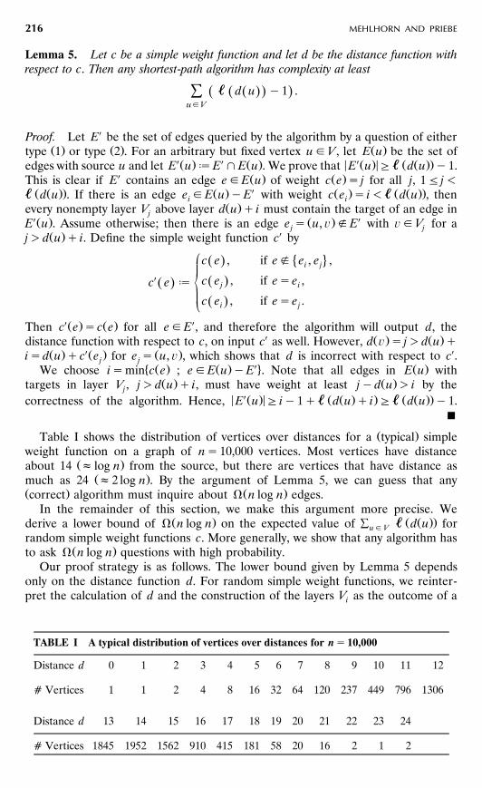
Lemma 5. Let c be a simple weight function and let d be the distance function withrespect to c. Then any shortest-path algorithm has complexity at least

,, d u y1 .Ž .Ž .Ž .ÝugV

Proof. Let EX be the set of edges queried by the algorithm by a question of eitherŽ . Ž . Ž .type 1 or type 2 . For an arbitrary but fixed vertex ugV, let E u be the set of

XŽ . X Ž . < XŽ . < Ž Ž ..edges with source u and let E u [E lE u . We prove that E u G,, d u y1.X Ž . Ž .This is clear if E contains an edge egE u of weight c e s j for all j, 1F j-

Ž Ž .. Ž . X Ž . Ž Ž ..,, d u . If there is an edge e gE u yE with weight c e s i-,, d u , theni iŽ .every nonempty layer V above layer d u q i must contain the target of an edge inj

XŽ . Ž . XE u . Assume otherwise; then there is an edge e s u, ¨ fE with ¨ gV for aj jŽ . Xj)d u q i. Define the simple weight function c by

¡ � 4c e , if ef e , e ,Ž . i j

X ~c e , if ese ,Ž .c e [Ž . j i¢c e , if ese .Ž .i j

XŽ . Ž . XThen c e sc e for all egE , and therefore the algorithm will output d, theX Ž . Ž .distance function with respect to c, on input c as well. However, d ¨ s j)d u q

Ž . XŽ . Ž . Xisd u qc e for e s u, ¨ , which shows that d is incorrect with respect to c .j j� Ž . Ž . X4 Ž .We choose ismin c e ; egE u yE . Note that all edges in E u with

Ž . Ž .targets in layer V , j)d u q i, must have weight at least jyd u ) i by thej

< XŽ . < Ž Ž . . Ž Ž ..correctness of the algorithm. Hence, E u G iy1q,, d u q i G,, d u y1.B

Ž .Table I shows the distribution of vertices over distances for a typical simpleweight function on a graph of ns10,000 vertices. Most vertices have distance

Ž .about 14 f log n from the source, but there are vertices that have distance asŽ .much as 24 f2 log n . By the argument of Lemma 5, we can guess that any

Ž . Ž .correct algorithm must inquire about V n log n edges.In the remainder of this section, we make this argument more precise. We

Ž . Ž Ž ..derive a lower bound of V n log n on the expected value of Ý ,, d u forug Vrandom simple weight functions c. More generally, we show that any algorithm has

Ž .to ask V n log n questions with high probability.Our proof strategy is as follows. The lower bound given by Lemma 5 depends

only on the distance function d. For random simple weight functions, we reinter-pret the calculation of d and the construction of the layers V as the outcome of ai

TABLE I A typical distribution of vertices over distances for ns10,000

Distance d 0 1 2 3 4 5 6 7 8 9 10 11 12

a Vertices 1 1 2 4 8 16 32 64 120 237 449 796 1306

Distance d 13 14 15 16 17 18 19 20 21 22 23 24

a Vertices 1845 1952 1562 910 415 181 58 20 16 2 1 2


random labeling process. Note that a random simple weight function is given by nindependent permutations of V, one for each vertex. The ith vertex of thepermutation for vertex ¨ is the target of the edge with weight i and source ¨ . The

� 4 Ž .labeling process proceeds in stages. In the zeroth stage, V is set to s and d s is0set to 0. In the ith stage, iG1, each vertex ¨ gS Ž i.sD V picks the0 F j- i jŽ Ž ..iyd ¨ th vertex in its adjacency list. Note that each vertex that ¨ has not yetseen is equally likely to occur. The newly reached vertices are put into V and theiri

d-values are set to i. Instead of fixing the n permutations before-hand, we may alsoŽ .view them as being fixed on-line principle of deferred decisions . This leads to the

following re-interpretation of the random labeling process: In the ith stage, eachvertex in S Ž i.sD V chooses a vertex uniformly and independently at ran-0 F j- i j

dom from the set of vertices it has not yet seen. The labeling process stops whenS Žk .sV for some k.

w xA related process was considered by Frieze and Grimmett in 7 . They assumedthat each vertex in S Ž i. chooses a vertex uniformly and independently at randomfrom the set of all vertices. If D denotes the number of stages taken by theirA

version of the process, then it is clear that D stochastically dominates D, i.e., forAŽ . Ž . w x Žall k, Pr D)k FPr D )k . Frieze and Grimmett prove in 7 that D andA A. Ž .hence D is O log n with high probability. However, we need a lower bound on D

Žand therefore their result is of no use to us. Nevertheless, our proof strategy was.inspired by theirs.

< Ž i. <The random labeling process is said to be in state j if S s j. We call stage i ofŽ i. '< <the labeling process central if nreF S Fny n . Layers constructed in central

stages are called central.Our proof will proceed in two steps. First, we show in Lemma 6 that there areŽ .V log n central stages with high probability. Second, we prove in Lemma 7 that

each central stage gives rise to a nonempty layer with high probability.

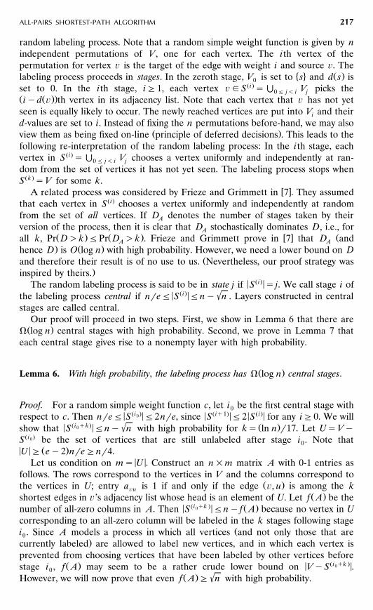
Ž .Lemma 6. With high probability, the labeling process has V log n central stages.

Proof. For a random simple weight function c, let i be the first central stage with0< Ž i0 . < < Ž iq1. < < Ž i. <respect to c. Then nreF S F2nre, since S F2 S for any iG0. We will

Ž i qk .0 '< < Ž .show that S Fny n with high probability for ks ln n r17. Let UsVyS Ž i0 . be the set of vertices that are still unlabeled after stage i . Note that0< < Ž .U G ey2 nreGnr4.

< <Let us condition on ms U . Construct an n=m matrix A with 0-1 entries asfollows. The rows correspond to the vertices in V and the columns correspond to

Ž .the vertices in U; entry a is 1 if and only if the edge ¨ , u is among the k¨ uŽ .shortest edges in ¨ ’s adjacency list whose head is an element of U. Let f A be the

< Ž i0qk . < Ž .number of all-zero columns in A. Then S Fny f A because no vertex in Ucorresponding to an all-zero column will be labeled in the k stages following stage

Ži . Since A models a process in which all vertices and not only those that are0.currently labeled are allowed to label new vertices, and in which each vertex is

prevented from choosing vertices that have been labeled by other vertices beforeŽ . < Ž i0qk . <stage i , f A may seem to be a rather crude lower bound on VyS .0 'Ž .However, we will now prove that even f A G n with high probability.


A row of A is a random 0-1 vector of length m with exactly k ones. Moreover,the row entries A , 1F iFn, are independent random variables, and if A, AX

i ?

< Ž . Ž X. <differ only in a single row, then f A y f A Fk. Hence, by Azuma’s inequalityŽ . Ž . Ž .Lemma 3 , we get the following tail estimate for f A s f A , . . . , A ,1 ? n ?

2 2Pr f A FE f A r2 F2 exp yE f A r 2nk . 11Ž . Ž . Ž . Ž . Ž .Ž . Ž .Ž .nThe probability that a fixed column is all-zero is 1ykrm ; therefore,

nkE f A sm 1y . 12Ž . Ž .ž /m

< < Ž . Ž . x y2Remember that ms U Gnr4 and ks ln n r17; since 1y1rx Ge for largeŽ .enough x, we get from 12 that

1y2 k n r m 1y8r17 'E f A Gme G n )2 n 13Ž . Ž .4

w Ž .x < <for large enough n, where E f A is conditioned on U sm. However, the lowerŽ .bound in 13 is independent of m. Hence,

21r17 yC'Pr f A - n F2 exp yQ n r ln n sO nŽ . Ž . Ž . Ž .Ž . Ž .< Ž i0qk . <for any fixed C)0 and large enough n. Since S is increasing in k, we have

Ž . Ž .thus proved that, with high probability, it will take V ln n sV log n central'stages to label all but n vertices. B

Ž .Remark. f A can be expressed as the sum of 0-1 indicator variables C , 1F jFm,jwhere C s1 if and only if column j of A is all-zero. The C ’s are not independent;j jfor example, Ý C Fmyk. However, they can be shown to be negati ely associated,j j

w xi.e., negatively dependent in a strong sense; see 3 for a proof. This property of theC ’s suffices to prove analogues of the Chernoff]Hoeffding bound from Lemma 2j

Ž . Ž .for the left tail of the distribution of f A , and 11 could be replaced by theŽ Ž . w Ž .x . yE w f Ž A.xr8sharper Pr f A FE f A r2 Fe .

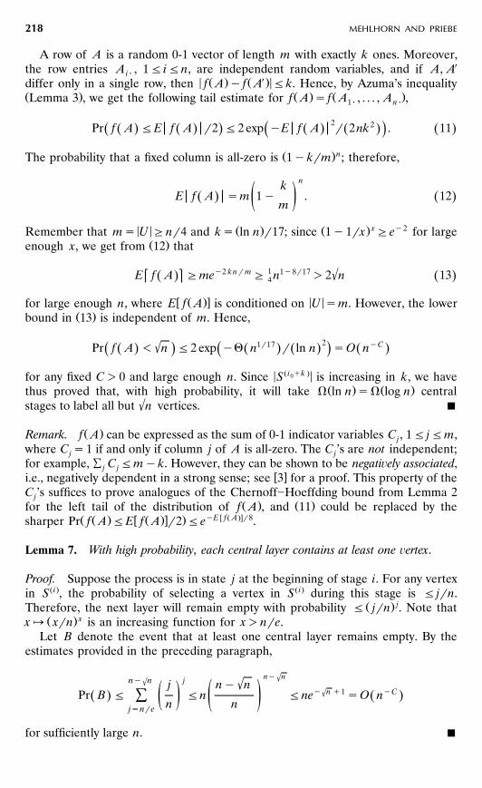
Lemma 7. With high probability, each central layer contains at least one ërtex.

Proof. Suppose the process is in state j at the beginning of stage i. For any vertexin S Ž i., the probability of selecting a vertex in S Ž i. during this stage is F jrn.

Ž . jTherefore, the next layer will remain empty with probability F jrn . Note thatŽ . xx¬ xrn is an increasing function for x)nre.

Let B denote the event that at least one central layer remains empty. By theestimates provided in the preceding paragraph,

ny n'jny n' 'j ny ny n q1 yC'Pr B F Fn Fne sO nŽ . Ž .Ý ž / ž /n njsnre

for sufficiently large n. B


Theorem 3. Any algorithm for the single-source shortest-path problem has complexityŽ .V n log n with high probability on random simple weight functions.

Proof. Suppose that i is the first central stage of the labeling process; as before,let S Ž i. denote the set of vertices that have already been labeled up to this stage. By

Ž .Lemma 6, with high probability, the process has V log n central layers. Lemma 7tells us that all these layers will be nonempty with high probability. With thenotation introduced in the discussion of the labeling process, this reads

,, d u y1 sV n log n with high probability.Ž . Ž .Ž .Ž .ÝŽ i.ugS

By Lemma 5, the left-hand side term is a lower bound on the complexity of anyshortest-path algorithm. B

ACKNOWLEDGMENTS

We learned from discussions with Paul Spirakis that analyzing the algorithm byw xMoffat and Takaoka 14 is not as easy as it might appear at first glance. The

remarks of Alistair Moffat and of an anonymous referee for ICALP’94 allowedconsiderable simplification of our proofs of Theorems 1 and 2. We are grateful tothe anonymous referees of this journal for their comments, especially for urging usto give a concise and sound presentation of both theorems. Rudolf Fleischersuggested the use of Fibonacci heaps in the implementation of the algorithm.Finally, numerous discussions with Hannah Bast and Torben Hagerup were partic-ularly insightful, and conversations with Devdatt Dubhashi and Shiva Chaudhurihelped to clarify our ideas.

This work was supported by the ESPRIT II Basic Research Actions Program ofŽ .the EC under contract number 7141 Project ALCOM II and the BMFT-Project

‘‘Softwareokonomie und Softwaresicherheit’’ ITS 9103. A preliminary version of¨this paper was presented at the Third Annual European Symposium on Algo-

w xrithms, Corfu, Greece, 1995, 12 . Volker Priebe’s research was supported by aGraduiertenkolleg graduate fellowship of the Deutsche Forschungsgemeinschaft.

REFERENCES

w x Ž 2 U .1 P. A. Bloniarz, A shortest-path algorithm with expected time O n log n log n , SIAMŽ .J. Comput., 12, 588]600 1983 .

w x2 E. W. Dijkstra, A note on two problems in connexion with graphs, Numer. Math., 1,Ž .269]271 1959 .

w x3 D. Dubhashi, V. Priebe, and D. Ranjan, Negative dependence through the FKGinequality, Research Report MPI-I-96-1-020, Max-Planck-Institut fur Informatik, Saar-¨brucken, August 1996.¨

w x Ž .4 R. W. Floyd, Algorithm 97: shortest path, Commun. ACM, 5, 345 1962 .w x5 M. L. Fredman, New bounds on the complexity of the shortest path problem, SIAM J.

Ž .Comput., 5, 83]89 1976 .


w x6 M. L. Fredman and R. E. Tarjan, Fibonacci heaps and their uses in improved networkŽ .optimization algorithms, J. ACM, 34, 596]615 1987 .

w x7 A. M. Frieze and G. R. Grimmett, The shortest-path problem for graphs with randomŽ .arc-lengths, Discrete Appl. Math., 10, 57]77 1985 .

w x8 W. Hoeffding, Probability inequalities for sums of bounded random variables, J. Am.Ž .Stat. Assoc., 58, 13]30 1963 .

w x9 M. Hofri, Analysis of Algorithms: Computational Methods and Mathematical Tools,Oxford University Press, Oxford, 1995.

w x10 D. R. Karger, D. Koller, and S. J. Phillips, Finding the hidden path: time bounds forŽ .all-pairs shortest paths, SIAM J. Comput., 22, 1199]1217 1993 .

w x11 C. McDiarmid, On the method of bounded differences, in Sur eys in Combinatorics,Ž .1989, J. Siemons, Ed. , London Mathematical Society Lecture Note Series 141,

Cambridge University Press, Cambridge, 1989, pp. 148]188.w x12 K. Mehlhorn and V. Priebe, On the all-pairs shortest path algorithm of Moffat and

Ž .Takaoka, in Algorithms}ESA ’95 P. Spirakis, Ed. , Lecture Notes in ComputerScience 979, Springer-Verlag, Berlin, 1995, pp. 185]198.

w x13 A. Moffat and T. Takaoka, An all pairs shortest path algorithm with expected runningŽ 2 .time O n log n , Proc. 26th Annual Symposium on Foundations of Computer Science,

Portland, OR, 1985, pp. 101]105.w x14 A. Moffat and T. Takaoka, An all pairs shortest path algorithm with expected time

Ž 2 . Ž .O n log n , SIAM J. Comput., 16, 1023]1031 1987 .w x15 R. Raman, The power of collision: randomized parallel algorithms for chaining and

integer sorting, in Foundations of Software Technology and Theoretical Computer Science,Ž .K. V. Nori and C. E. Veni Madhavan, Eds. , Lecture Notes in Computer Science 472,Springer-Verlag, Berlin, 1990, pp. 161]175.

w x16 P. M. Spira, A new algorithm for finding all shortest paths in a graph of positive arcs inŽ 2 2 . Ž .average time O n log n , SIAM J. Comput., 2, 28]32 1973 .

w x17 T. Takaoka, A new upper bound on the complexity of the all pairs shortest pathŽ .problem, Inf. Process. Lett., 43, 195]199 1992 .

w x18 H. Thorisson, Coupling methods in probability theory, Scand. J. Stat., 22, 159]182Ž .1995 .

Documents

On the all-pairs shortest-path algorithm of Moffat and Takaoka