ON TACTILE SENSING AND DISPLAY

A DISSERTATION

SUBMITTED TO THE DEPARTMENT OF MECHANICAL ENGINEERING

AND THE COMMITTEE ON GRADUATE STUDIES

OF STANFORD UNIVERSITY

IN PARTIAL FULFILLMENT OF THE REQUIREMENTS

FOR THE DEGREE OF

DOCTOR OF PHILOSOPHY

William R. ProvancherAugust 2003

ii

© Copyright 2003 by William R. ProvancherAll Rights Reserved

iii

I certify that I have read this dissertation and that in my opinion it is fully adequate, in scope and quality, as a dissertation for the degree of Doctor of Philosophy.

Mark R. Cutkosky, Principal Advisor

I certify that I have read this dissertation and that in my opinion it is fully adequate, in scope and quality, as a dissertation for the degree of Doctor of Philosophy.

Kenneth J. Waldron

I certify that I have read this dissertation and that in my opinion it is fully adequate, in scope and quality, as a dissertation for the degree of Doctor of Philosophy.

Thomas W. Kenny

Approved for the University Committee on Graduate Studies.

iv

Abstract

With the aid of telerobotics it has become possible to manipulate an object across the world

or even on another planet. But how can the user feel what the remote robot hand is touch-

ing? The challenges associated with displaying tactile sensations are formidable, requiring

the ability to recreate changing contact geometries, pressure distributions and vibrations at

the user's fingertips. Despite years of research, telerobotic consoles provide their operators

mainly with visual feedback and overall handling forces. The experience is akin to manip-

ulating an object with fireplace tongs. The goal of the research presented herein is to extend

the capabilities of current systems by imparting tactile sensations to their users.

This thesis presents new methods of tactile sensing and display for dexterous tele-

manipulation, i.e., telemanipulation that involves imparting forces and motions with the

fingertips. The motivating hypothesis for this work is that sensing and displaying contact

location provides essential information for dexterous telemanipulation. A new tactile

sensor is presented that consists of an array of curvature-measuring elements. The curva-

ture measurements provide information for manipulation planning and control and provide

an estimate of the local object geometry, useful for grasp stability analysis. The approach

is validated in simulation and experimentally.

The companion to the sensor is a display that allows users to track finger/object con-

tact locations. The tactile display renders the location of the contact centroid on a user's fin-

gertip and thereby provides the user with cues about object motion and curvature. The

ability of users to discriminate among different object curvature and motion conditions is

investigated in a series of experiments involving real and virtual objects rendered via the

display. The results indicate that contact location provides an important cue for dexterous

telemanipulation and that, for gently curved objects, the performance of users with the dis-

play is comparable to their performance when they touch objects directly with their own

fingertips.

v

For Pam

Acknowledgments

The path to a Ph.D. has been a long and winding one. The route was not always well illuminated, but there have been many people who provided guidance and support along the way. I am grateful for their time, friendship, and words of wisdom.

I’d like to start by thanking my advisor, Mark Cutkosky. You took a chance on me by allowing a “composites guy” with no robotics experience to work in your lab. Because of this opportunity, I have learned and grown as an engineer and a researcher. I’d also like to thank the members of my reading and defense committees: Chris Chafe, Tom Kenny, Günter Niemeyer, and Ken Waldron. Thanks for your suggestions, they were instrumental in my completing this work.

I’ve been fortunate enough to work with the extremely talented and friendly members of the Dexterous Manipulation Lab. I had only a brief overlap with some of the previous members of the lab: Turner, Costa, Allison and Chris, but they helped me get started on the right track. As for the current members, I don't know where to begin. Sean, Weston, Jonathan, Moto, Arthur-Trey, Karpick, Dan, Miguel, Kevin, Eric, Sangbae and Li, it’s been great getting to know all of you. I am especially indebted to Weston and Sean. I will miss our late afternoon “sugar breaks.” Weston, you have always been quick to lend a help-ing hand. Sean, your critical eye was not always welcome, but it is greatly appreciated.

I’d like to express my gratitude to Dr. Herb Rauch. Thanks for your help and patience in developing the formal mathematical model for my sensor and your tremendous effort in editing and proofreading the paper I presented at ISER02. It was also particularly well timed.

I’ve also benefited from a foster research group in Günter Niemeyer’s Telerobotics Lab. Vanessa and Katherine, because of your hard work the contact location experiments actually came to life in RTai Linux. Katherine, I particularly appreciate the many late nights you put in and your diligence in coping with the hiccups along the way. Günter,

vi

vii

thanks for playing “devil’s advocate” in our many philosophical discussions about contactdisplays and experiments.

I want to thank researchers from the “haptics community” for their many suggestions.My discussions with Susan Lederman, Rob Howe and Mandayam Srinivason were enlight-ening and helped me in thinking through the contact display experiments.

I’d also like to acknowledge the staff of CDR: Judy Lee, Jeff Aldrich and AlisonKather, for their administrative, behind the scenes support.

Thanks to James Hetfield and Chris Cornell for inspiration and Puma for entertain-ment. They really got me through the rough times.

I’d like to thank my parents and my brother, Jason, for supporting me over the years. Iwant to thank the Beilkes and Despreses, each of whom have been a surrogate family tome. Thanks also to Andre, Paul, Rob, and John for being good friends over the years. Mostof all I’d like to thank my wife, Pam, for her endless encouragement and forgiving mybeing late for dinner.

I’d also like to acknowledge the National Science Foundation that supported myresearch under grant NSF/IIS-0099636.

Contents

CHAPTER 1. Introduction......................................................................................... 11.1 Motivation ........................................................................................................... 21.2 Contributions ...................................................................................................... 21.3 Thesis Outline ..................................................................................................... 3

CHAPTER 2. Human Tactile Sensing and Perception............................................ 42.1 Human Mechanoreception .................................................................................. 42.2 Psychophysics ..................................................................................................... 7

2.2.1 Standard Psychophysical Protocol and Interpretation .............................. 82.2.1.1 Weber’s Law ..................................................................................... 9

2.2.2 Classical Psychophysical Methods to Establish JNDs ........................... 102.2.2.1 Method of Constant Stimuli ............................................................ 102.2.2.2 Method of Limits ............................................................................. 162.2.2.3 Method of Adjustment ..................................................................... 16

CHAPTER 3. Shape Sensor: A Tactile Sensor for Measuring Object Geometry183.1 Previous Work .................................................................................................. 183.2 Sensor Concept ................................................................................................. 19

3.2.1 Data Fitting Approach ............................................................................ 203.3 Sensor Design and Construction ....................................................................... 23

3.3.1 Design Trades ......................................................................................... 233.3.2 Sensor Operational Theory ..................................................................... 273.3.3 Sensor Electronics .................................................................................. 323.3.4 Sensor Construction ................................................................................ 35

3.4 Simulation ......................................................................................................... 373.4.1 Two-Dimensional Simulation of Surface ............................................... 37

3.4.1.1 Two-Dimensional Reference Surface .............................................. 373.4.1.2 Two-Dimensional Simulation Results ............................................. 38

3.4.2 One-Dimensional Simulation of Planar Curve ....................................... 403.4.2.1 One-Dimensional Reference Surface .............................................. 403.4.2.2 One-Dimensional Simulation Results ............................................. 41

3.4.3 Discussion of Simulation Results ........................................................... 433.5 Experimental Validation ................................................................................... 43

3.5.1 Experimental Procedure ......................................................................... 433.5.1.1 Calibration and Hysteresis Testing .................................................. 433.5.1.2 Centered Line Load Test ................................................................. 44

3.5.2 Experimental Results and Discussion .................................................... 443.5.2.1 Calibration and Hysteresis Testing .................................................. 443.5.2.2 Centered Line Load Test ................................................................. 47

viii

3.6 Conclusions ....................................................................................................... 48

CHAPTER 4. Contact Location Display ................................................................. 504.1 Previous Work .................................................................................................. 52

4.1.1 Vertically Moving Pin Arrays ................................................................ 534.1.2 Laterally Moving Pin Arrays .................................................................. 554.1.3 Electrotactile Arrays ............................................................................... 554.1.4 Passive Arrays ........................................................................................ 56

4.2 Device Design ................................................................................................... 564.3 Experimental Goals and Approach ................................................................... 61

4.3.1 General Experimental Protocol .............................................................. 614.4 Curvature Discrimination for Real and Virtual Objects ................................... 63

4.4.1 Experimental Procedure ......................................................................... 634.4.2 Results and Discussion of Curvature Discrimination Experiments ....... 65

4.5 Perception of Object Motion ............................................................................ 714.5.1 Experimental Procedure ......................................................................... 724.5.2 Results and Discussion of Object Motion Experiments ......................... 73

4.6 General Discussion and Conclusions ................................................................ 75

CHAPTER 5. Extensions and Conclusions ............................................................. 775.1 Summary of Contributions ............................................................................... 775.2 Improvements and Extensions .......................................................................... 78

5.2.1 Tactile Sensor ......................................................................................... 795.2.2 Contact Location Display ....................................................................... 80

5.3 Conclusion ........................................................................................................ 82

APPENDIX A. Sensor Bridge Circuitry and Thermal Modelling......................... 83

A.1 Strain Gage Bridge Circuitry ........................................................................... 83A.2 Sensor Thermal Modelling .............................................................................. 87

A.2.1 Thermal Modelling Results ................................................................... 87A.2.1.1 Sensor Warm-up with Asymmetric Boundary Conditions ............. 88A.2.1.2 Imbalance in Gage Resistance ........................................................ 89A.2.1.3 Operating Sensor in Cold Environment .......................................... 90A.2.1.4 Contact with a Cold Object ............................................................ 92A.2.1.5 Inhomogeneous Substrate Conduction ........................................... 92

A.2.2 Summary of Thermal Modelling Results .............................................. 93

APPENDIX B. Contact Location Display Design Details ....................................... 94

B.1 Early Prototype Designs ................................................................................... 94B.2 Details of Current Design ................................................................................ 97

B.2.1 Actuator Assembly ................................................................................ 98B.2.2 Thimble Assembly ............................................................................... 100

B.2.2.1 Thimble Design ............................................................................. 100B.2.3 Push-Pull Wire Assemblies ................................................................. 103

B.3 Device Performance ....................................................................................... 105

ix

APPENDIX C. Kinematics for Curvature Discrimination Experiments............ 107

Bibliography............................................................................................................. 112

x

Tables

CHAPTER 1. .................................................................................................................. 1

CHAPTER 2. .................................................................................................................. 4

Table 2-1. Characteristics of mechanoreceptors found in human fingertip skin (sensed parameters suggested by Johnson and Phillips 1981, Johansson, Landstrom, and Lundstrom 1982 and Vallbo and Johansson 1984). ................................................................................ 6

CHAPTER 3. ................................................................................................................ 18

Table 3-1. Sources of electrical noise in sensor measurements. Both pre- and post- amplification sources of electrical noise are given. The pre-amplification noise is combined and this resultant is amplified as reported. Note that the dominant noise sources are from the reference diode used to generate the bridge excitation voltage and A/D conversion......................................................................................... 34

Table 3-2. Major sources of sensor drift. Drift primarily affects the sensor gain and therefore the sensor accuracy. Estimates for sensor drift are based on a 1% strain level in the gages and a 20°C drop in operating temperature. ...................................................................................... 34

Table 3-3. Simulation results for a 10 cm x 10 cm surface patch with a 10 x 10 array of curvature measuring elements subjected to various load conditions ......................................................................................... 40

Table 3-4. Simulation results for a center loaded inextensional curved beam with a 10 x 1 array of curvature measuring elements with 12.9 mm radius.. 41

Table 3-5. Experimental results for center loaded sensor. Results are presented in increasing order of the magnitude of center deflection. ................... 47

CHAPTER 4. ................................................................................................................ 50

Table 4-1. Results of direct and virtual radius of curvature perception experiments in the form of JNDs and Weber fractions for each curvature standard. The right side of the table shows length-based results for virtual discriminations. .................................................... 68

CHAPTER 5. ................................................................................................................ 77

APPENDIX A. .............................................................................................................. 83

xi

Table A-1. Material properties relevant to sensor thermal modeling. ................ 88Table A-2. Parameter values used in thermal models. ....................................... 88

APPENDIX B. .............................................................................................................. 94

Table B-1. Percentile fingertip sizes (source: The Measure of Man and Woman [Dreyfuss 2002])............................................................................. 101

APPENDIX C. ............................................................................................................ 107

xii

Figures

CHAPTER 1. .................................................................................................................. 1

CHAPTER 2. .................................................................................................................. 4Figure 2-1. Cross-section of human fingertip skin showing four types of

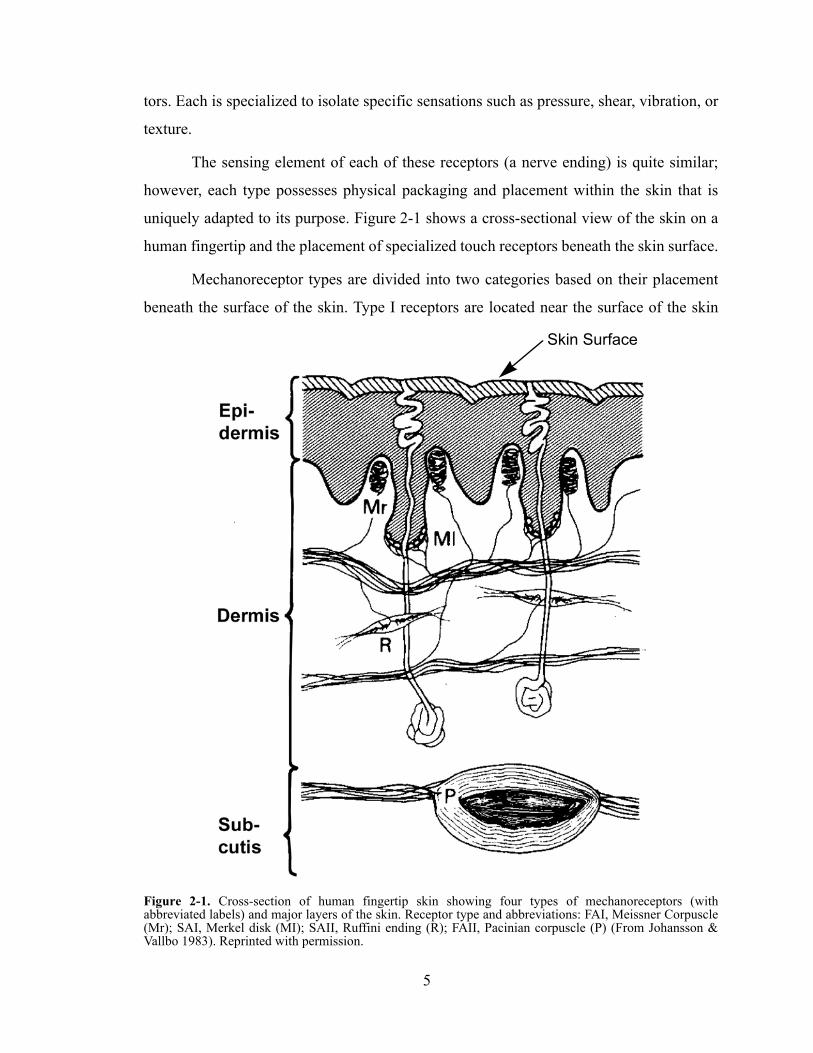
mechanoreceptors (with abbreviated labels) and major layers of the skin. Receptor type and abbreviations: FAI, Meissner Corpuscle (Mr); SAI, Merkel disk (MI); SAII, Ruffini ending (R); FAII, Pacinian corpuscle (P) (From Johansson & Vallbo 1983). Reprinted with permission. ................... 5

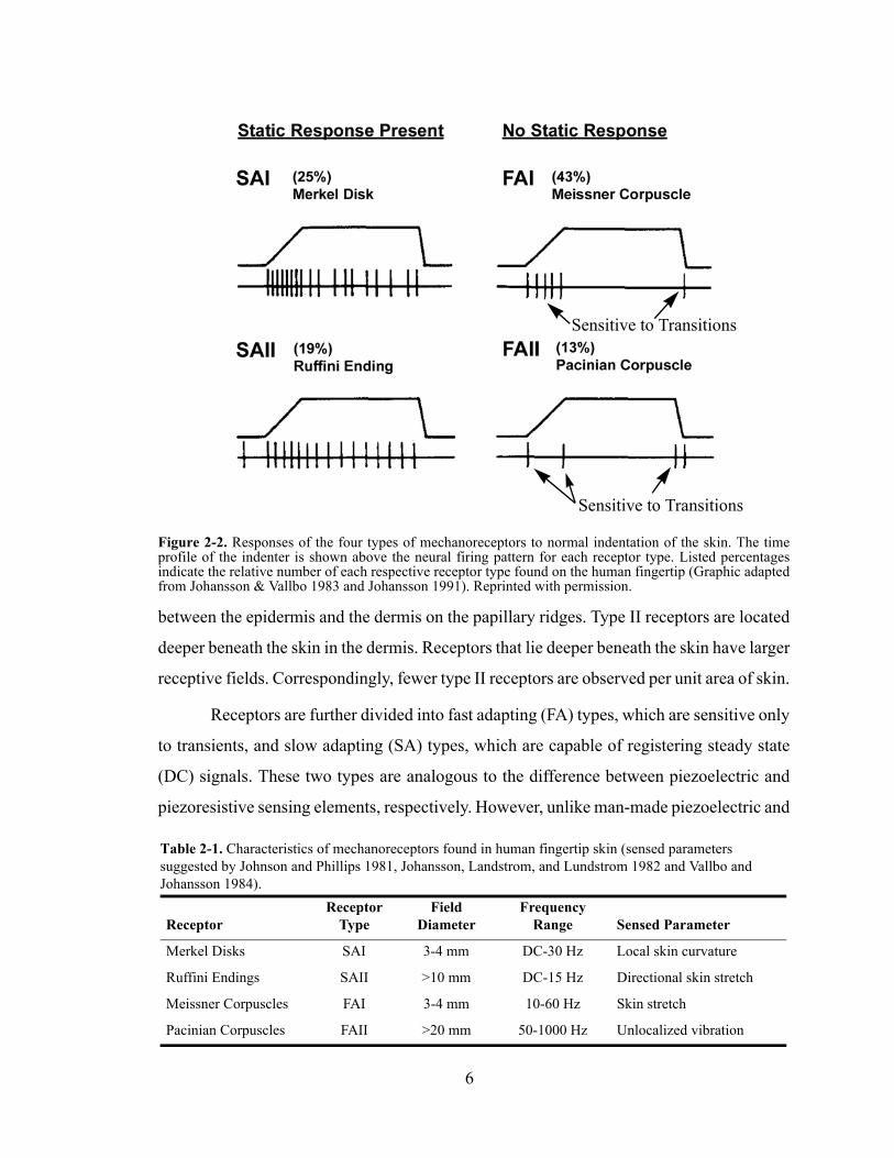
Figure 2-2. Responses of the four types of mechanoreceptors to normal indentation of the skin. The time profile of the indenter is shown above the neural firing pattern for each receptor type. Listed percentages indicate the relative number of each respective receptor type found on the human fingertip (Graphic adapted from Johansson & Vallbo 1983 and Johansson 1991). Reprinted with permission............................................................................ 6

Figure 2-3. Graph of a S-shaped psychometric function. The proportion represents the number of times a stimulus is chosen divided by the times it is presented. The shape of the curve is derived from the fact that psychophysical measurements tend to be normally distributed. The interpretation for the reported proportion and shape of the right side of the curve (i.e., for the comparison stimuli that are larger than the standard) is illustrated in Figures 2-4(a), (b), and (c). Similar reasoning can be used to explain the reported proportions and shape of the left side of the curve (i.e., for the stimuli that are smaller than the standard).................................................. 12

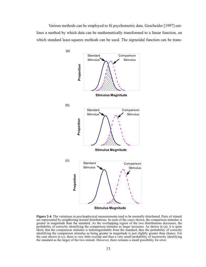
Figure 2-4. The variations in psychophysical measurements tend to be normally distributed. Pairs of stimuli are represented by neighboring normal distributions. In each of the cases shown, the comparison stimulus is greater in magnitude than the standard. As the overlapping region of the two distributions decreases, the probability of correctly identifying the comparison stimulus as larger increases. As shown in (a), it is quite likely that the comparison stimulus is indistinguishable from the standard, thus the probability of correctly identifying the comparison stimulus as being greater in magnitude is just slightly greater than chance. For the case shown in (c), there is very little overlap and thus a very small probability of incorrectly identifying the standard as the larger of the two stimuli. However, there remains a small possibility for error. .......................................................... 13

Figure 2-5. Methodology of curve fit for typical data. 1) Sigmoidal curve fit established by converting proportions to z-scores. 2) Once converted to z-scores, a line is fit to the data by the method of least squares (shown in (b)). 3) The sigmoidal curve fit results from converting the linear fit back to equivalent proportions (shown in (a)). ......................................................................... 15

CHAPTER 3. ................................................................................................................ 18Figure 3-1. Schematic of sensor construction and typical results for a linear sensor

prototype..................................................................................................... 19

xiii

Figure 3-2. General (n x m) parametric surface patch. Detail of local surface shows curvature sensing element kij which indicates curvature of the ijth point. 20

Figure 3-3. Sensor thermal conduction model overlaid on detailed cross-section of the sensor. The model is useful for predicting the operation temperature of the gage elements, as well as for investigating events that could result in a temperature differential between the gages of a half-bridge. ..................... 25

Figure 3-4. Sensor thermal conduction model. Electrical circuit representation of the sensor thermal model. The thermal equations of motion describe the dynamic behavior of the sensor. Tg1 and Tg2 are the temperatures of the outboard and inboard gages, respectively. T0 is the ambient temperature - also assumed to be the temperature of the sensor base. Tobj is the temperature of an object touched by the sensor. Rsub,X1 and Rsub,X2 are the through-thickness thermal resistance of the substrate for outboard and inboard gages, respectively. Rskin,X1 is the thermal resistance of heat flowing from the outboard strain gage to the silicone skin and Rsub,Y is the thermal resistance for heat dissipation into the polyimide substrate. Csub,Y is the heat capacity of the polyimide substrate. Rskin,X1 represents the thermal resistance of heat flowing from the outboard strain gage to the silicone skin and Rskin,Y is the thermal resistance for heat dissipation into the silicone skin. Cskin,Y is the heat capacity of the silicone skin. Rskin,X2 is the through-thickness thermal resistance of the silicone rubber skin, which is important when the sensor comes in contact with hot or cold objects.. This value of this resistance is set to infinity when the sensor is not in contact. 26

Figure 3-5. Schematic of sensor half-bridge used to measure curvature. ..................... 28Figure 3-6. (a) Cross-sectional view of sensor pressed against an object of radius, robj.

(b) Relevant dimensions of the sensor substrate and strain gages viewed with sensor array flattened and in cross-section. (c) The radius of curve is measured and computed at the mid-line of the substrate, rave, which can be related to the radius of curvature of the object, robj, by accounting for the substrate, gage, and membrane thicknesses, ts, tg , and tm , respectively.. 29

Figure 3-7. Sensor array electrical schematic. .............................................................. 32Figure 3-8. Sensor array construction for the (a) first- and (b) second-generation

prototypes. .................................................................................................. 35Figure 3-9. Second generation sensor prototype. (a) Top and (b) bottom of two-sided

flex circuit are shown. ................................................................................ 36Figure 3-10. Second generation sensor shown as it would be packaged at the fingertip of a

telerobot...................................................................................................... 36Figure 3-11. Mesh plots for various load cases. For each load case, the reference surface

is shown on the left and the surface fit to data with simulated noise is shown on the right. The load cases presented are: (a) Centered Point Load, (b) Off-center point load, and (c) Skewed line load. The reference surface for each load case was generated using a 15th order Fourier sine series (see Timoshenko & Gere 1961). See Table 3-3 for numerical results. .............. 39

Figure 3-12. Line plots for a centered loaded inextensional curved beam. Results are presented for increasing magnitude of center deflection. Reference curves are shown with the solid line while the curve fit to data with simulated noise is indicated with the dashed line in each graph. ......................................... 42

Figure 3-13. Sensor calibration and quantification of mechanical hysteresis for second generation strain gage array prototype. (a) Sensor held against known singly-curved surface. (b) Calibration data for all gage-pairs. (c) Calibration data

xiv

for a single gage-pair (5th gage-pair). (d) Averaged calibration data for all gage-pairs. Some hysteresis is evident in each graph, as the data form an open loop rather than falling on a straight line........................................... 46

Figure 3-14. Plot of reconstructed shape for centered loaded sensor based on measured curvature ..................................................................................................... 48

CHAPTER 4. ................................................................................................................ 50Figure 4-1. a) Concept for contact location display. The centroid of contact is

represented with a single tactile element. (a) Two-dimensional and (b) one-dimensional variations are illustrated......................................................... 51

Figure 4-2. Solid Model of the contact location display. (a) Side view of the device and close-ups of the (b) thimble and (c) actuator. ............................................. 56

Figure 4-3. a) Prototype of contact location display. Contacts are rendered by a roller housed in a thimble. The roller is attached to a commercial force-feedback device to provide reaction forces to the finger. A small servo-motor provides precise positioning of the roller via push-pull wires. The roller is suspended below the finger, only touching the user when interaction forces are displayed by the PhantomTM. b) Experimental setup and graphics showing a contact between the user's finger and a virtual object. ............................... 57

Figure 4-4. The illusion of making and breaking contact with virtual objects is enhanced as the tactile element is brought into contact with the user’s finger when making contact. Experimental graphics are shown along with solid models and pictures of the thimble in analogous states. (a) In free-space, the roller remains separated from the user’s finger. (b) Interaction forces, supplied by the haptic feedback device, bring the roller into contact with the users finger when making contact with virtual objects. ................................................. 58

Figure 4-5. Contact display control diagram. Motions of the contact were driven as a function of finger position, xF. Finger position was calculated from known Phantom™/roller position, xR, and contact display leadscrew position, xC. As shown in (a) xF = xR - xC. (b) Controller block diagram. The desired Phantom™/roller position was driven by a kinematic contact model. For example, for object motion experiments, the reference input, R(s) = a · xF. Controller design and graphics are shown courtesy of Katherine J. Kuchenbecker of the Stanford Telerobotics Lab.................... 60

Figure 4-6. (a) One-fingered planar perception of curvature provides a simplified form of object manipulation and highlights the use of contact location while exploring an object's geometry. (b) The experiments were performed exploring 15° sectors of a "curvature wheel" for the direct manipulation. An arm rest, that could roll horizontally, helped users maintain horizontal motion. (c) Experiment graphics used during initial training. ................... 64

Figure 4-7. Pooled results of all subjects for radius of curvature discriminations during (a) direct physical interaction and (b) simulated virtual interaction rendered via the contact location display. The graphs display the proportion of times a particular stimulus was reported as having a greater radius of curvature. The JNDs are indicated with dotted lines. ......................................................... 66

Figure 4-8. Methodology of curve fit for typical data. Sigmoidal curve fit established by converting proportions to z-scores (abscissa) of a "standard normal distribution4." Once converted to z-scores, a line is fit to the data by the method of least squares (shown in (b)). The sigmoidal curve fit results from converting the linear fit back to equivalent proportions (shown in (a)). .... 67

xv

Figure 4-9. JNDs of direct and virtual radius of curvature discrimination tests are plotted versus their nominal stimuli value.............................................................. 68

Figure 4-10. Radius and equivalent length JNDs for virtual discrimination tests. ......... 69Figure 4-11. Results are framed by data reported in the literature for active fingertip

curvature discrimination (Gordon and Morison [1982]) and passive discrimination (Goodwin et al. [1991]). ..................................................... 70

Figure 4-12. Differences in apparent object motion can be described in terms of a ratio, a = DXO/DXF , where DXO is the object displacement and DXF is the fingertip displacement. Values of a for familiar object motions are depicted above. ......................................................................................................... 72

Figure 4-13. Graphics for object motion experiment...................................................... 73Figure 4-14. The graphs display the proportion of times a given object motion ratio was

reported as being (a) rolling or (b) anchored. The means of the rolling and anchored object distributions are 0.56 and -0.09, respectively................... 74

CHAPTER 5. ................................................................................................................ 77

APPENDIX A. .............................................................................................................. 83Figure A-1. (a) Wheatstone bridge and specialized configurations (b-d) to measure

bending strain. A list of attributes are given for each. The half-bridge configuration has many advantages over the quarter-bridge, and requires fewer gages than the full-bridge. ................................................................ 84

Figure A-2. (a) Voltage divider circuit and (b) half-bridge configuration of Wheatstone bridge used to measure curvature. .............................................................. 86

Figure A-3. Sensor warm-up from ambient (25°C). A slight temperature differential between the inner and outer gages results from asymmetric thermal boundary conditions. This asymmetry is a result of the protective silicone rubber skin on the sensor. The steady-state temperature differential is 0.14°C. ........... 89

Figure A-4. Effect of operating the sensor at 5°C. This has little effect on the steady state temperature differential, which is 0.14°C. However, there are other consequences that should be considered (see discussion in section A.2.1.3).. 90

Figure A-5. Effect of touching a cold (5°C) object. This has only a slight effect on the temperature differential between the gages. The steady state temperature differential is 0.17°C, only a 0.03°C difference from nominal (refer to Figure A-3 for nominal warm-up).............................................................. 91

Figure A-6. Effect of increasing the thermal resistance of the inner gage heat flow into the substrate by ten-fold has only a slight effect on the temperature differential between the gages. The steady state temperature differential is 0.84°C. This is 0.7°C difference from the nominal warm-up temperature imbalance (refer to Figure A-3 for nominal warm-up). ............................. 92

APPENDIX B. .............................................................................................................. 94Figure B-1. Proof of concept prototype made from a 3.5 inch floppy disk drive

mechanism. (a) Side view of device. The actuator is grounded to the middle phalynx of the index finger by a foam lined ring. The picture shown in (b) provides a view of the device from the top and back sides and (c) provides a view of the device from the front. .............................................................. 94

xvi

Figure B-2. Custom prototype of contact location display mounting to middle phalynx of index finger. (a) Side view of prototype shown with longer motor for increased torque and torsion spring to apply contact force for the roller. (b) and (c) show the device from alternate angles. .......................................... 96

Figure B-3. a) Prototype of the contact location display. The roller is attached to a commercial force-feedback device to provide reaction forces to the finger. A small servo-motor provides precise positioning of the roller via push-pull wires. The roller is suspended below the finger, only touching the user when interaction forces are displayed by the PhantomTM.................................. 97

Figure B-4. Actuator assembly. A leadscrew couples the motion of the motor to the push-pull wires. The device is calibrated by driving the carriage against a small contact switch at startup. ............................................................................ 98

Figure B-5. Thimble assembly. The thimble was produced by FDM and coated in epoxy. It is lined with foam for comfort and to accommodate small variations in user’s finger sizes. .................................................................................... 100

Figure B-6. Orthogonal layout of thimble design with relevant dimensions............... 102Figure B-7. A family of thimbles were used to accommodate the wide range of finger

sizes. The thimbles are lined with 1/6 inch, 1/8 inch, or 3/16 inch PVC foam tape. The thimbles also differ based on the vertical offset from the bottom of the user’s finger to the centerline of the push-pull wires. ........................ 103

Figure B-8. Push-pull wire assembly. (a) Sava push-pull wire assembly. The ends of the nylon sheath are press-fit into center-drilled 10-32 cap screws. (b) Custom designed push-pull wire assembly with teflon sheath. The center-drilled cap screws were bonded to the ends of the Tefon® sheaths. (c) and (d) show a close-up of the sheath bonded into the center-drilled 10-32 cap screws. . 104

Figure B-9. Performance plots for the contact display device. (a) Tracking plot for the device rendering a stationary object. The desired position is based on the motion of the user’s finger. (b) Device response to a 2 mm step input. The response is slightly underdamped with a 50 ms rise time. In contrast to (a) plots (c) and (d) were generated by driving the roller with a sinusoid with the user’s hand stationary. (c) Tracking plot for the contact display driven by a 5 Hz sine wave with 1 cm peak-to-peak amplitude. (d) Tracking plot for the contact display driven by a 8 Hz sine wave with 1 cm peak-to-peak amplitude. As seen in plot (d), there is considerable lag as the tracking performance falls off. The small motion bandwidth of the device is approximately 8 Hz. Plots shown courtesy of Katherine J. Kuchenbecker of the Stanford Telerobotics Lab................................................................... 106

APPENDIX C. ............................................................................................................ 107Figure C-1. Schematic representation of the virtual object motion in curvature

discrimination experiments. Virtual objects were constrained to follow an arc, pivoting about the origin. The curvature stimuli were small circular disks inscribed on a circular wheel of radius, Rw. Only x and y motions of the virtual finger were allowed (no rotation), so object kinematics can be described purely as a function of finger position, given some initial configuration. ........................................................................................... 108

xvii

1 Introduction

We use our hands every day to assess the size, shape, and texture of objects. We sense and

interpret tactile stimuli from our environment and perform tasks with our hands in a nearly

instinctual manner. The ability to discriminate among surface textures, sense incipient slip,

and roll an object between fingers without dropping it can be attributed to the specialized

mechanoreceptors in the hand. These touch receptors possess unrivaled range and acuity.

They respond to both static and dynamic stimuli as well as temperature and pain. We are

also equipped with reflexes and automatic responses (e.g., grasp force regulation) that

allow us to make use of tactile information without expending cognitive effort. Despite the

obvious importance of tactile cues in our everyday lives, the subject of tactile display for

teleoperators, virtual reality, and more generally, human/machine interfaces, has only

recently received significant attention.

This thesis presents new methods of tactile sensing and display. The goal of this

research is to bring the level of tactile sensitivity and acuity that humans possess to telema-

nipulators and other human/machine interfaces. A new method for measuring local object

geometry is presented based on an array of curvature measurements. Such information is

indispensable for coordinating finger motions for object manipulation. Unfortunately, it is

more the exception than the rule that even a portion of this information is relayed to tele-

operators. Devising a device to display the full sensation of contact continues to elude

researchers. Most commonly, researchers will present an abstraction of contact geometry

and pressure with a pin array display. These devices recreate a reasonable facsimile of

shape at the contact, but their large package size makes them impractical for use outside the

laboratory. The method of displaying contact presented herein, represents a further abstrac-

tion. Rather than presenting the shape of the contact, a more minimalist approach of

displaying only its centroid is proposed. Packaging and actuation requirements for this

approach are modest in comparison to previous approaches. Results of experiments with

1

human subjects demonstrate that it provides them with cues necessary to ascertain object

curvature and motion capabilities.

1.1 MotivationTo date, telemanipulation systems have relied heavily on vision feedback and have required

experienced operators. It has been shown, however, that adding the sense of touch to these

systems connects the operator to the remote environment, making the system more intuitive

[Dennerlein et al. 1997, Sheridan 1992].

Similarly, for virtual reality, when advanced graphics and sound are augmented by

force and vibration feedback, one's perception is altered and one becomes immersed in an

artificial reality [Burdea 1996].

Perhaps even more important than the sense of realism that tactile feedback creates

is its ability to leverage innate human tactile ability. With tactile sensation at their fingertips

humans can bring their extensive experience in handling objects to bear on the problem at

hand. In areas where touch is extremely important, such as medicine, we create the ability

for telesurgeons to palpate and probe biological tissue as if they were touching it with their

own hands.

1.2 ContributionsThe major contributions of this thesis are:

• A new sensor and mathematical framework for measuring local object geometry via

an array of curvature measurements are presented. The sensor is analyzed and its

inherent accuracy and sensitivity are determined numerically and in experiments.

• A new approach to tactile display based on displaying the centroid of contacts for

telemanipulation and virtual reality is developed and tested.

• Evaluation of human perception of contact location feedback in prototypical manipu-

lation tasks is conducted.

• Thresholds for cutaneous length-based perception, as used in rolling objects between

the fingers, are determined.

2

1.3 Thesis OutlineThis thesis is organized into five chapters. This chapter provides an introduction to and

motivation for my research in tactile sensing and display and lists the contributions of this

work.

Chapter 2 provides relevant background in human tactile sensing and perception.

The physical parameters and role of human mechanoreception are outlined. This chapter

also provides an overview of methods from psychophysics that are useful for evaluating

human performance and the effectiveness of new haptic devices. Specific attention is given

to the methods employed in the tests reported in chapter 4.

Chapter 3 introduces an approach for sensing local object geometry via an array of

curvature measurements and reviews previous tactile array sensor technologies. An

approach for surface reconstruction using Fourier series basis functions is presented and

validated by simulation and experiments. A prototype incorporating a linear array of cur-

vature measuring elements was fabricated to experimentally validate the design. Sensor

design, construction and experimental results are presented. Additional background on

sensor circuitry and thermal modeling is provided in Appendix A.

Chapter 4 reviews the design of current tactile displays and introduces the idea of

displaying only the location of the centroid of contacts to users of telemanipulation and vir-

tual reality systems. A prototype that renders contacts along the length of a single finger

was designed and fabricated to investigate the approach. The device was mounted to a force

feedback device to render environmental interaction forces. Human subject testing was

conducted with virtual environments to evaluate the device and the user’s relevant percep-

tion. The contact location display design and test hardware are presented along with results

of initial device evaluation in human subjects experiments. Additional details of the device

design can be found in Appendix B. An in-depth derivation of the kinematics used in the

curvature discrimination experiments can be found in Appendix C.

Chapter 5 summarizes the results of this research and suggests future extensions of

this work.

3

2 Human Tactile Sensing and Perception

Designing hardware meant to convey artificial touch to the human hand is a significant

challenge. The primary reason is that our hands are incredibly sensitive to even the slightest

vibrations over a range from 10-100 Hz. To help define the design requirements of such

hardware, it is crucial to understand underlying tactile sensing mechanisms. Not only will

this serve as a source of inspiration for improving tactile sensor designs, it will also help

focus on which signals are important to communicate and how to communicate them.

Although this is requisite knowledge, there is more to consider than simply the neurophys-

iology of touch. Our sense of touch is really a fusion of tactile and kinesthetic information.

The combination of cutaneous and kinesthetic sensing is referred to as haptic perception.

At a high level, it is the perception or interpretation of these signals that ultimately interests

us.

A field of cognitive psychology, psychophysics, provides methods well suited for

understanding haptic perception. Researchers in psychophysics have developed specialized

methods for quantifying perceived sensations that accompany physical stimuli, thus pro-

viding a systematic approach for evaluating human performance and the effectiveness of

new hardware and implementations. The remainder of this chapter provides an overview of

human mechanoreception and psychophysics and outlines methods used to evaluate human

tactile ability.

2.1 Human MechanoreceptionThe human hand contains a complex array of specialized receptors that are rugged enough

to survive repeated impacts, while retaining the ability to detect faint vibrations and the

softest touch. Neurophysiologists have identified four main types of tactile mechanorecep-

4

tors. Each is specialized to isolate specific sensations such as pressure, shear, vibration, or

texture.

The sensing element of each of these receptors (a nerve ending) is quite similar;

however, each type possesses physical packaging and placement within the skin that is

uniquely adapted to its purpose. Figure 2-1 shows a cross-sectional view of the skin on a

human fingertip and the placement of specialized touch receptors beneath the skin surface.

Mechanoreceptor types are divided into two categories based on their placement

beneath the surface of the skin. Type I receptors are located near the surface of the skin

Figure 2-1. Cross-section of human fingertip skin showing four types of mechanoreceptors (with abbreviated labels) and major layers of the skin. Receptor type and abbreviations: FAI, Meissner Corpuscle (Mr); SAI, Merkel disk (MI); SAII, Ruffini ending (R); FAII, Pacinian corpuscle (P) (From Johansson & Vallbo 1983). Reprinted with permission.

Skin Surface

5

between the epidermis and the dermis on the papillary ridges. Type II receptors are located

deeper beneath the skin in the dermis. Receptors that lie deeper beneath the skin have larger

receptive fields. Correspondingly, fewer type II receptors are observed per unit area of skin.

Receptors are further divided into fast adapting (FA) types, which are sensitive only

to transients, and slow adapting (SA) types, which are capable of registering steady state

(DC) signals. These two types are analogous to the difference between piezoelectric and

piezoresistive sensing elements, respectively. However, unlike man-made piezoelectric and

Figure 2-2. Responses of the four types of mechanoreceptors to normal indentation of the skin. The time profile of the indenter is shown above the neural firing pattern for each receptor type. Listed percentages indicate the relative number of each respective receptor type found on the human fingertip (Graphic adapted from Johansson & Vallbo 1983 and Johansson 1991). Reprinted with permission.

Sensitive to Transitions

Sensitive to Transitions

Table 2-1. Characteristics of mechanoreceptors found in human fingertip skin (sensed parameters suggested by Johnson and Phillips 1981, Johansson, Landstrom, and Lundstrom 1982 and Vallbo and Johansson 1984).

ReceptorReceptor

TypeField

DiameterFrequency

Range Sensed Parameter

Merkel Disks SAI 3-4 mm DC-30 Hz Local skin curvature

Ruffini Endings SAII >10 mm DC-15 Hz Directional skin stretch

Meissner Corpuscles FAI 3-4 mm 10-60 Hz Skin stretch

Pacinian Corpuscles FAII >20 mm 50-1000 Hz Unlocalized vibration

6

piezoresistive sensors, which provide analog signals, biological mechanoreceptors encode

their signals as a series of pulses (as shown in Figure 2-2), similar to digital serial commu-

nication. Table 2-1 gives a summary of the characteristics of each mechanoreceptor and the

physical parameters they measure.

For a more thorough review of tactile sensing mechanisms, see Johansson and

Vallbo [1983] or Vallbo and Johansson [1984] (available on Johansson’s Laboratory of

Dexterous Manipulation website, http://www.humanneuro.physiol.umu.se/). For a review

of research specifically related to the encoding of shape and curvature, such as that reported

in section 4.4, see Srinivasan and LaMotte [1991] (available on the MIT Touch Lab web-

site, http://touchlab.mit.edu/).

2.2 PsychophysicsPsychophysics is a subfield of cognitive psychology. It arose out of the desire to quantify

the relationship "between sensations in the psychological domain and stimuli in the physi-

cal domain" [Gescheider 1997]. It was pioneered in the 1800’s by the German scientists E.

H. Weber and G. T. Fechner, who were interested in determining sensory thresholds for

human perception.

Measuring such thresholds is central to psychophysics. Researchers in this field

have measured both absolute and relative thresholds for nearly every imaginable sensory

modality (hearing, vision, touch...). The absolute threshold refers to the minimum stimulus

necessary to be registered as a perceptible sensation, whereas a relative or difference

threshold (JND: Just Noticeable Difference), represents the minimum difference necessary

to distinguish between two signals. An example of an absolute threshold could be the min-

imum amplitude of vibration (at a given frequency) necessary to perceive a vibration. In

contrast, one might determine a JND based on the minimum necessary variation in ampli-

tude, about some reference stimulus magnitude, necessary to distinguish between two

vibratory signals of a given frequency.

As mentioned previously, the determination of absolute and difference thresholds is

central to psychophysics; however, they represent only two of the four paradigms of psy-

chophysics that could be exploited to evaluate haptic performance (the other two are rec-

7

ognition and scaling, which will not be addressed here). For a general introduction to

psychophysics, including a review of established testing methods and procedures, see

Gescheider [1997]. For a review of research focused specifically on human tactile sensing,

see Loomis and Lederman [1986], and Schiff and Foulke [1982].

One interesting side note from this reading is that researchers have found a differ-

ence in tactile thresholds based on whether they were determined through active or passive

touch. This can be an important consideration when constructing and interpreting psycho-

physical experiments [Loomis and Lederman 1986]. This is particularly relevant to the

experiments in curvature discrimination presented in section 4.4, and will be discussed in

more detail along with the experimental results. The remainder of this section provides a

brief introduction to some of the concepts and methods that are germane to the experiments

described in chapter 4.

2.2.1 Standard Psychophysical Protocol and InterpretationThe field of psychophysics includes well-established procedures and protocol specifically

designed to measure human perception of physical stimuli. These procedures were estab-

lished to reduce the possibility of introducing systematic bias into test procedures. The tests

described in chapter 4 were constructed based on standard psychophysical protocol.

These tests employed a paired-comparison, forced-choice protocol, which is also

the standard protocol used in an eye exam. The optometrist presents the patient with a series

of comparisons, asking the subject to state which lens is more in focus (“Here’s lens ‘A’,

and here’s lens ‘B’.”). There are several sources of error and bias, which are often order-

based. For this reason, after honing in on the proper prescription, the optometrist will often

invert the order of presentation of a pair of lenses. Likewise, standard protocol for estab-

lishing JNDs dictates that each combination of stimuli must be presented an even number

of times, where the order of presentation is inverted half of the time.

The occurrence of presentation-order bias (also called a time error) is quite

common and takes several forms. A time error results from the fact that there is always a

small delay between the presentation of the comparison and standard stimuli. One example

of this type of error is when the comparison is judged larger than the standard a larger pro-

portion of the time when the comparison stimulus is presented second. One interpretation

8

of this is that the memory of the first sensation fades with time, leaving a diminished

memory of the sensation to compare with the more recent stimulus. This often leads sub-

jects to identify the second stimulus as larger, even if it is not the case.

In addition to balancing presentation order to prevent order bias for sequentially

presented stimuli, it is important to balance testing order within a test session (especially as

test length increases). This reduces the influence of learning and fatigue in determining

thresholds. Note, however, that one can also examine these groups separately (i.e., JNDs

for standards completed at the beginning of the test versus at the end) to determine whether

learning or fatigue had a substantial effect.

Another source of bias results from the nature of making sequential presentations

of stimuli. It is difficult to ensure that the stimuli are judged by the same exact receptors;

thus, this type of error is referred to as a space error. Though a space error is less of an issue

when determining audible thresholds, it can be a concern for touch-based experiments. On

the other hand, some of these concerns can be mitigated by increasing the number of test

trials and by testing a broad number of human subjects.

2.2.1.1 Weber’s LawIt is interesting to examine the relationship between stimulus intensity and the correspond-

ing JND. For a wide range of stimulus values, the JND is proportional to the stimulus inten-

sity. This phenomenon was first observed by E. H. Weber when conducting experiments

with weights [Gescheider 1997]. He found that as the mass of the standard increased, so did

the incremental mass (JND) that subjects required to discern the difference between the

standard and comparison stimuli. In examining data across a broad range, Weber found the

JND to be linearly related to the stimulus intensity (stimulus magnitude). Weber’s law, rear-

ranged in the form of the Weber fraction, is shown below.

(2.1)

This relationship holds over a wide range of sensory modalities and is useful for making

comparisons within data sets, though it should be noted that this law breaks down as the

intensity of the stimuli approaches the absolute threshold (see Gescheider [1997]).

Weber Fraction JNDStimulus Intensity------------------------------------------------=

9

2.2.2 Classical Psychophysical Methods to Establish JNDsIn classical psychophysics there are three primary methods that are used to evaluate per-

ceptual thresholds: the method of constant stimuli, the method of limits, and the method of

adjustment. The experiments presented in chapter 4 establish difference thresholds (JNDs)

for curvature and motion, so the description of each of these methods will be expressed with

that goal in mind, though it should be noted that these methods can also be used to measure

absolute thresholds. Each of these methods has its own merits that should be considered

when establishing a testing methodology. The following subsections provide a description

of each of these methods and note some of the advantages and disadvantages of each. The

greatest attention is given to the method of constant stimuli because it is the method that

was used for the experiments described in chapter 4.

2.2.2.1 Method of Constant StimuliIn this method, a set of constant stimuli are repeatedly presented to test subjects. Typically,

stimuli are presented on the order of one hundred times each to establish JNDs. Quite often,

experiments are conducted on only a few individuals, necessitating multiple testing ses-

sions; however, one could also pool data from multiple subjects to reduce the time commit-

ment of each subject.

To establish a difference threshold (JND), a set of predetermined comparison stim-

uli are presented in combination with a standard stimulus (the reference point about which

the differences of the comparison stimuli are judged). The comparison stimuli are both

greater and smaller in size than the standard stimulus and should be equally spaced (as a

general rule, at least six comparison stimuli should be used, three smaller and three larger).

Subjects will decide which of the presented stimuli has the particular characteristic of inter-

est (e.g., which is larger).

Preliminary testing is helpful in establishing a range over which the largest of the

comparison stimuli is almost always identified as being larger and the smallest of the com-

parison is almost never mistaken as being larger than the standard stimulus. It should be

noted that with all psychophysical testing it is essential to make preliminary test runs (pilot

tests) to verify appropriateness of procedures and selection of proper test stimuli before

investing considerable time in gathering test data.

10

Each time a particular stimulus is selected, it is recorded to determine the proportion

of times each stimulus is chosen:

(2.2)

The proportion is the number of times that each stimulus is judged as being larger than the

standard divided by the number of times that that stimulus is presented. For each stimulus,

the proportion is plotted against its associated intensity/magnitude, resulting in a graph

called a psychometric function. It should be noted that even though the standard is not com-

pared to a stimulus of identical magnitude, it is compared to both stimuli of greater and

smaller magnitude. Therefore, we expect that half of the time the standard will be identified

as the larger. Whereas the other data points show the judgement on how an individual com-

parison stimulus relates to the standard, the data point which corresponds to the magnitude

of the standard reflects judgements of the standard with respect to the entire stimulus set.

Note that slight deviations from a proportion of 0.5 are expected for the standard, due to

possible bias.

These graphs typically resemble an S-shaped curve as shown in Figure 2-3. Fitting

an S-shaped curve to points of the psychometric function is supported by theory and exper-

imental findings across many sensing modalities [Gescheider 1997]. The shape of this

curve is related to the fact that variations in psychophysical measurements tend to be nor-

mally distributed. The S-shaped curve is a cumulative form of this distribution. This is illus-

trated schematically in Figure 2-4 for the case of three distinct comparison stimuli. In each

graph in this figure, two signals are shown (i.e., the standard and comparison stimuli), each

represented by a normal distribution.

One can see that if the two signals are of similar magnitude, as in Figure 2-4(a), that

there is a large region of overlap between the two distributions. A large region of overlap

means that there is a greater possibility for error (interpreting the two stimuli as equal or

even interpreting the smaller signal as the larger of the two stimuli). As the difference

between the two signals becomes greater, the overlapping region is reduced, and the likeli-

hood of correctly identifying the relative magnitude of the two stimuli increases. As shown

in Figure 2-4(a), it is quite likely that the comparison stimulus is indistinguishable from the

Proportion Number of Times ChosenNumber of Times Presented---------------------------------------------------------------------------=

11

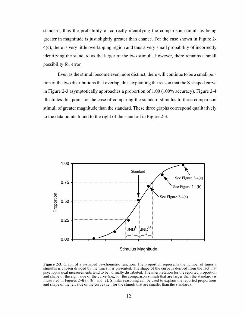
standard, thus the probability of correctly identifying the comparison stimuli as being

greater in magnitude is just slightly greater than chance. For the case shown in Figure 2-

4(c), there is very little overlapping region and thus a very small probability of incorrectly

identifying the standard as the larger of the two stimuli. However, there remains a small

possibility for error.

Even as the stimuli become even more distinct, there will continue to be a small por-

tion of the two distributions that overlap, thus explaining the reason that the S-shaped curve

in Figure 2-3 asymptotically approaches a proportion of 1.00 (100% accuracy). Figure 2-4

illustrates this point for the case of comparing the standard stimulus to three comparison

stimuli of greater magnitude than the standard. These three graphs correspond qualitatively

to the data points found to the right of the standard in Figure 2-3.

0.00

0.25

0.50

0.75

1.00

20 30 40 50 60Stimulus Magnitude

Pro

porti

on

JNDL JNDU

Figure 2-3. Graph of a S-shaped psychometric function. The proportion represents the number of times a stimulus is chosen divided by the times it is presented. The shape of the curve is derived from the fact that psychophysical measurements tend to be normally distributed. The interpretation for the reported proportion and shape of the right side of the curve (i.e., for the comparison stimuli that are larger than the standard) is illustrated in Figures 2-4(a), (b), and (c). Similar reasoning can be used to explain the reported proportions and shape of the left side of the curve (i.e., for the stimuli that are smaller than the standard).

Standard

See Figure 2-4(a)

See Figure 2-4(b)

See Figure 2-4(c)

12

Various methods can be employed to fit psychometric data. Gescheider [1997] out-

lines a method by which data can be mathematically transformed to a linear function, on

which standard least-squares methods can be used. The sigmoidal function can be trans-

Stimulus Magnitude

Prop

ortio

n

StandardStimulus

ComparisonStimulus

Figure 2-4. The variations in psychophysical measurements tend to be normally distributed. Pairs of stimuli are represented by neighboring normal distributions. In each of the cases shown, the comparison stimulus is greater in magnitude than the standard. As the overlapping region of the two distributions decreases, the probability of correctly identifying the comparison stimulus as larger increases. As shown in (a), it is quite likely that the comparison stimulus is indistinguishable from the standard, thus the probability of correctly identifying the comparison stimulus as being greater in magnitude is just slightly greater than chance. For the case shown in (c), there is very little overlap and thus a very small probability of incorrectly identifying the standard as the larger of the two stimuli. However, there remains a small possibility for error.

(a)

(b)

(c)

Stimulus Magnitude

Prop

ortio

n

StandardStimulus

ComparisonStimulus

Stimulus Magnitude

Prop

ortio

n

StandardStimulus

ComparisonStimulus

13

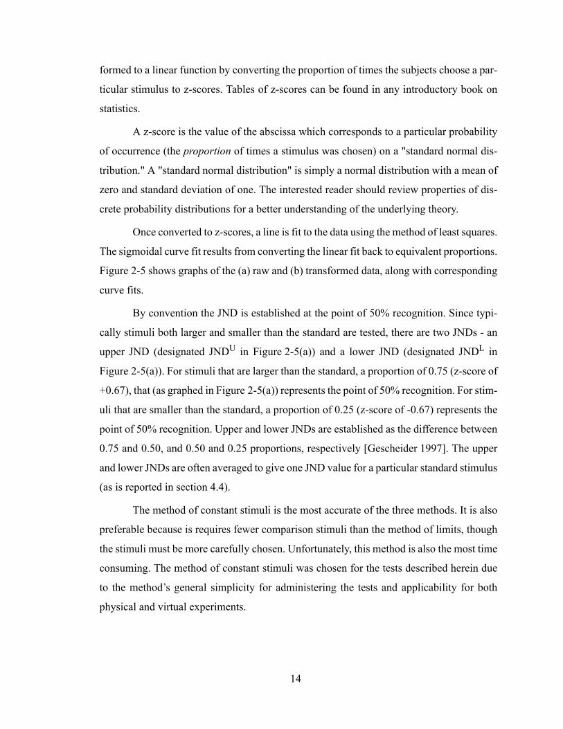
formed to a linear function by converting the proportion of times the subjects choose a par-

ticular stimulus to z-scores. Tables of z-scores can be found in any introductory book on

statistics.

A z-score is the value of the abscissa which corresponds to a particular probability

of occurrence (the proportion of times a stimulus was chosen) on a "standard normal dis-

tribution." A "standard normal distribution" is simply a normal distribution with a mean of

zero and standard deviation of one. The interested reader should review properties of dis-

crete probability distributions for a better understanding of the underlying theory.

Once converted to z-scores, a line is fit to the data using the method of least squares.

The sigmoidal curve fit results from converting the linear fit back to equivalent proportions.

Figure 2-5 shows graphs of the (a) raw and (b) transformed data, along with corresponding

curve fits.

By convention the JND is established at the point of 50% recognition. Since typi-

cally stimuli both larger and smaller than the standard are tested, there are two JNDs - an

upper JND (designated JNDU in Figure 2-5(a)) and a lower JND (designated JNDL in

Figure 2-5(a)). For stimuli that are larger than the standard, a proportion of 0.75 (z-score of

+0.67), that (as graphed in Figure 2-5(a)) represents the point of 50% recognition. For stim-

uli that are smaller than the standard, a proportion of 0.25 (z-score of -0.67) represents the

point of 50% recognition. Upper and lower JNDs are established as the difference between

0.75 and 0.50, and 0.50 and 0.25 proportions, respectively [Gescheider 1997]. The upper

and lower JNDs are often averaged to give one JND value for a particular standard stimulus

(as is reported in section 4.4).

The method of constant stimuli is the most accurate of the three methods. It is also

preferable because is requires fewer comparison stimuli than the method of limits, though

the stimuli must be more carefully chosen. Unfortunately, this method is also the most time

consuming. The method of constant stimuli was chosen for the tests described herein due

to the method’s general simplicity for administering the tests and applicability for both

physical and virtual experiments.

14

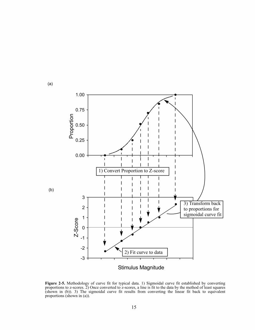
Figure 2-5. Methodology of curve fit for typical data. 1) Sigmoidal curve fit established by converting proportions to z-scores. 2) Once converted to z-scores, a line is fit to the data by the method of least squares (shown in (b)). 3) The sigmoidal curve fit results from converting the linear fit back to equivalent proportions (shown in (a)).

(a)

(b)

-3

-2

-1

0

1

2

3

20 30 40 50 60Stimulus Magnitude

Z-S

core

0.00

0.25

0.50

0.75

1.00

20 30 40 50 60Stimulus Magnitude

Pro

porti

on

1) Convert Proportion to Z-score

3) Transform backto proportions forsigmoidal curve fit

2) Fit curve to data

15

2.2.2.2 Method of LimitsIn the method of limits, a series of stimuli are presented to test subjects in an ascending or

descending order. To establish a JND, the stimuli are paired with a standard stimulus. Ini-

tially, testing begins by presenting stimuli well above or well below the standard, so that it

is easily distinguished from the standard. For an ascending series, the value of the compar-

ison stimuli is increased by small increments until it can no longer be distinguished from

the standard. After recording this point, testing continues (incrementing the value of the

comparison stimuli) until the subject can once again distinguish a difference between the

standard and comparison stimuli. This results in a gap over which the subjects can not dis-

cern the difference between the two stimuli. The JND is established as half of the width of

this gap.

The process is repeated several times for each standard. To help reduce the possi-

bility of habituation (e.g., always choosing the stimulus presented fourth), the series are run

in both ascending and descending order for each standard. Each series should also begin at

a slightly different comparison value, though care should be taken not to start with a value

too far from the standard, as this could extend test time and lead to disinterest and fatigue.

The method of limits is less time consuming and generally more popular than the

method of constant stimuli. While it is not as accurate as the method of constant stimuli, it

is more accurate than the method of adjustment. However, the large number of comparisons

in this method necessitates having a large number of comparison stimuli. This is undesir-

able if the fabrication of test stimuli is difficult or time consuming. This was not the case

for the experiments presented in chapter 4; however, it would have presented a logistical

issue to accurately present this many physical stimuli in rapid succession (since the method

of constant stimuli requires only seven stimuli per test, these stimuli could easily be fit

around the perimeter of the "curvature wheel" (see Figure 4-6), thus simplifying the pre-

sentation of stimuli).

2.2.2.3 Method of AdjustmentThis method is quite similar to the method of limits; however, in the method of adjustment,

the test subjects themselves adjust the value of the comparison stimuli to match the stan-

dard. Subjects complete many trials for each standard, and though some scatter in the data

16

is expected, they should nominally cluster around the value of the standard. For this

method, a measure of the dispersion of the data, such as its standard deviation, is used as

the JND. Precautions similar to those mentioned for the method of limits can be employed

to reduce habituation.

Researchers have presented mixed views about this method. Some argue that the

extra dimension of control afforded to test subjects can help to reduce boredom and apathy.

However, others believe that this can put undue pressure on the test subjects. Furthermore,

it must be possible to format the test such that it can be self-administered. The bottom line

is that the method can proceed quite rapidly, but is acknowledged to be less accurate than

the other two methods.

17

3 Shape Sensor: A Tactile Sensor for Measuring Local Object Geometry

Dexterous manipulation in humans and in robots requires information about the contact

conditions between the fingertips and a grasped object. For example, when rolling an object

between the fingertips, the curvature of the object and the locations of contacts on the finger

and object surfaces must be known to plan the required finger motions. Other surface prop-

erties such as friction and compliance also influence the manipulation strategy. In humans,

such information is obtained through a combination visual and tactile sensing and is essen-

tial for skillful object handling.

In robots, despite many years of research, the state of the art in tactile sensing and

interpretation is comparatively primitive. The challenge of creating a sensate artificial

"skin" for robotic hands is formidable. Trade-offs must inevitably be made among spatial

resolution, robustness, pressure sensitivity and the ability to comply with irregular or

curved surfaces. Providing power and transporting signals along the robot fingers are also

difficult, especially when the digits are human-sized or smaller. Nonetheless, many kinds

of tactile sensors have been reported in the literature.

The following sections present previous work in tactile sensing, the conceptual

approach of the sensor, the sensor design and construction, and the results of simulations

and experiments. The chapter concludes with a discussion of the results.

3.1 Previous WorkNumerous examples of tactile sensors exist in the literature. For reviews of the state of the

art in robotic tactile sensing see Dario [1991], Lee [2000], Maeno [2002] and Petriu et al.

[2002]. However, more specifically we find that others have also made estimates of object

curvature and shape as discussed in this chapter. Notably, Fearing and Binford [1991] used

18

Hertzian contact models as the basis of their pressure-based estimates. Rucci and Dario

[1994] and Canepa et al. [1992], used a piezoresistive tactile array and neural network to

measure object curvature. Charlebois et al. [1997] used position estimates from a tactile

sensor to estimate local shape.

In most implementations, the tactile sensors consist of an array of pressure or pres-

sure and shear-sensing elements [Fearing and Binford 1991, Chang 1995]. The compliance

of these sensors can be tailored but, in general, cannot accommodate large deformations.

However, other researchers starting with Brocket [1985] have argued the merits of soft

robotic fingertips consisting of a skin covering an inner layer of liquid or foam. With these

sensors, it becomes more practical to measure deformations of the skin rather than pressure

and shear stress distributions. Nowlin [1991], Russel [1992], and Ferrier and Brocket

[2000] present tactile sensors of this type. The salient characteristic of these sensors is that

they measure deflections of the skin and, with suitable processing, can provide measure-

ments of local object geometry. Thus, in addition to the practical advantages afforded by

soft fingertips [Shimoga and Goldenberg 1996], they provide information that is of direct

use for planning dexterous motions with rolling and/or sliding. A difficulty with previous

soft-finger designs, however, is that they pose challenging numerical problems to recon-

struct the skin geometry from (noisy) sensor readings.

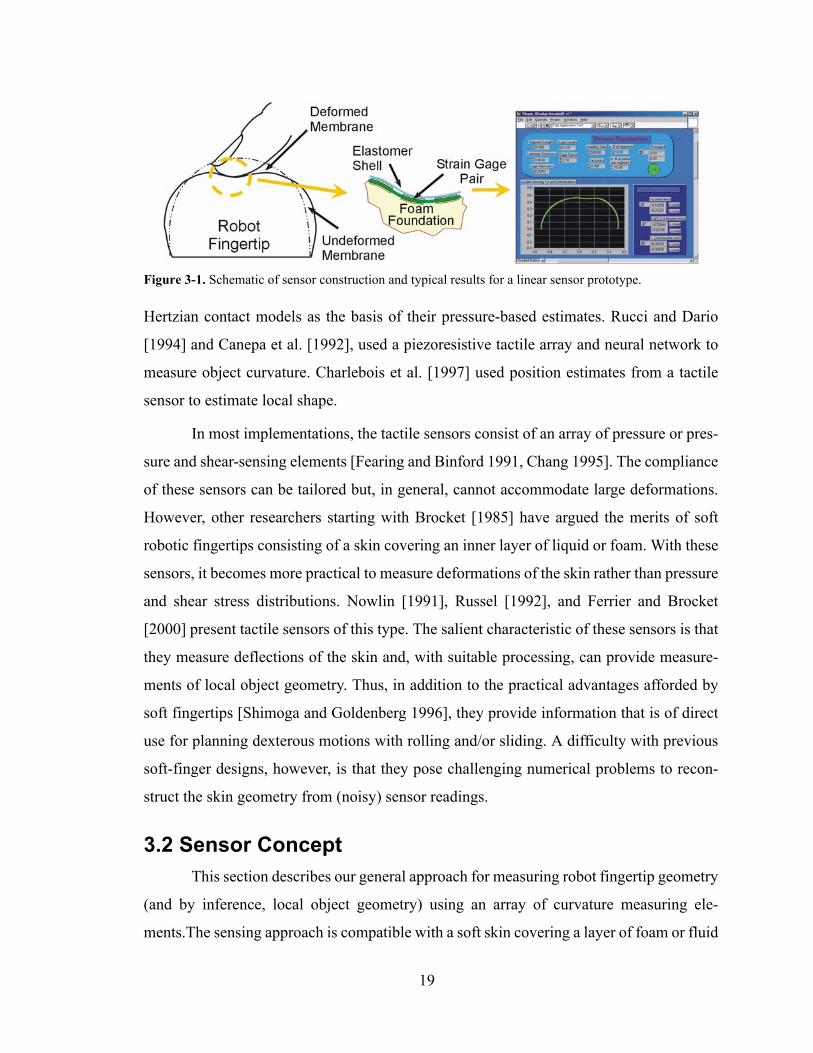
3.2 Sensor ConceptThis section describes our general approach for measuring robot fingertip geometry

(and by inference, local object geometry) using an array of curvature measuring ele-

ments.The sensing approach is compatible with a soft skin covering a layer of foam or fluid

Figure 3-1. Schematic of sensor construction and typical results for a linear sensor prototype.

19

(Figure 3-1) and allows the skin geometry to be reconstructed with a minimum of compu-

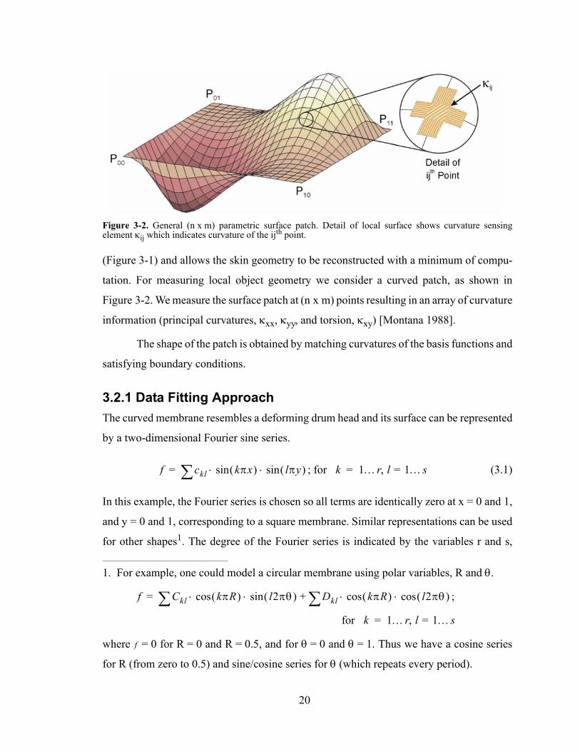
tation. For measuring local object geometry we consider a curved patch, as shown in

Figure 3-2. We measure the surface patch at (n x m) points resulting in an array of curvature

information (principal curvatures, κxx, κyy, and torsion, κxy) [Montana 1988].

The shape of the patch is obtained by matching curvatures of the basis functions and

satisfying boundary conditions.

3.2.1 Data Fitting ApproachThe curved membrane resembles a deforming drum head and its surface can be represented

by a two-dimensional Fourier sine series.

; for (3.1)

In this example, the Fourier series is chosen so all terms are identically zero at x = 0 and 1,

and y = 0 and 1, corresponding to a square membrane. Similar representations can be used

for other shapes1. The degree of the Fourier series is indicated by the variables r and s,

1. For example, one could model a circular membrane using polar variables, R and θ.

;

for

where = 0 for R = 0 and R = 0.5, and for θ = 0 and θ = 1. Thus we have a cosine series

for R (from zero to 0.5) and sine/cosine series for θ (which repeats every period).

Figure 3-2. General (n x m) parametric surface patch. Detail of local surface shows curvature sensing element κij which indicates curvature of the ijth point.

f ckl kπx( ) lπy( )sin⋅sin⋅∑= k 1…r l 1…s=,=

f Ckl kπR( ) l2πθ( )sin⋅cos⋅∑ Dkl kπR( ) l2πθ( )cos⋅cos⋅∑+=

k 1…r l 1…s=,=

f

20

which are generally equal. And as a two-dimensional series is used, r2 coefficients are

required to describe the sensor surface. Generally, the accuracy of the reconstruction

improves by choosing a higher order for the Fourier series, but should not exceed the

number of sensor measurements to avoid numerical difficulties.

The curvature measurements, κxx, κyy and κxy are related to the surface deformation

by the following equations:

(3.2)

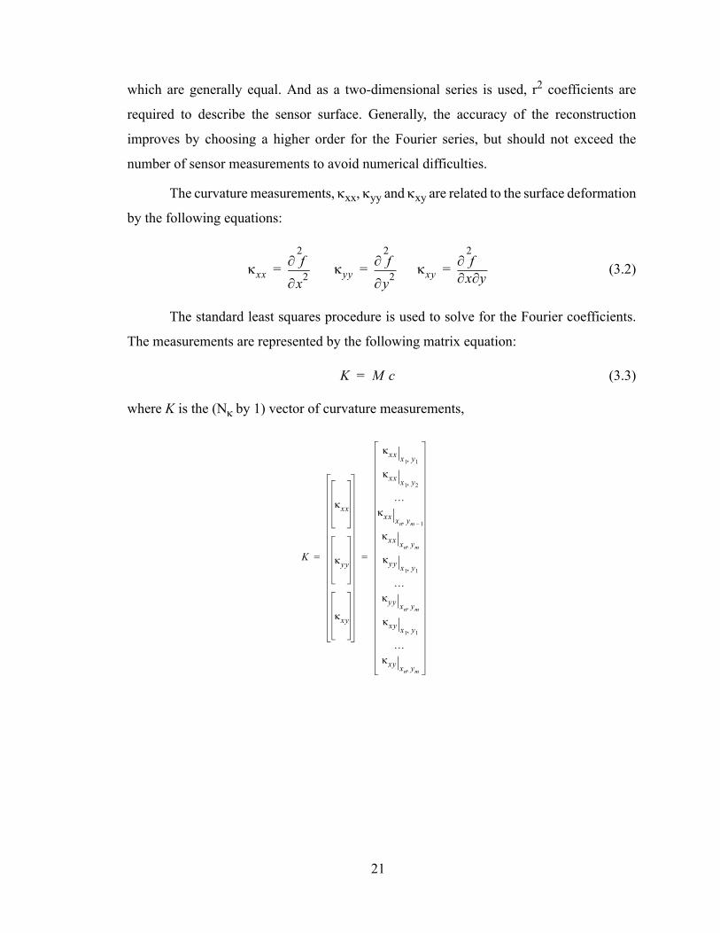
The standard least squares procedure is used to solve for the Fourier coefficients.

The measurements are represented by the following matrix equation:

(3.3)

where K is the (Nκ by 1) vector of curvature measurements,

κxxx2

2

∂

∂ f= κyyy2

2

∂

∂ f= κxy x y∂

2

∂∂ f=

K M c=

K

κxx

κyy

κxy

κxx x1 y1,

κxx x1 y2,

…κxx xn ym 1–,

κxx xn ym,

κyy x1 y1,

…κyy xn ym,

κxy x1 y1,

…κxy xn ym,

= =

21

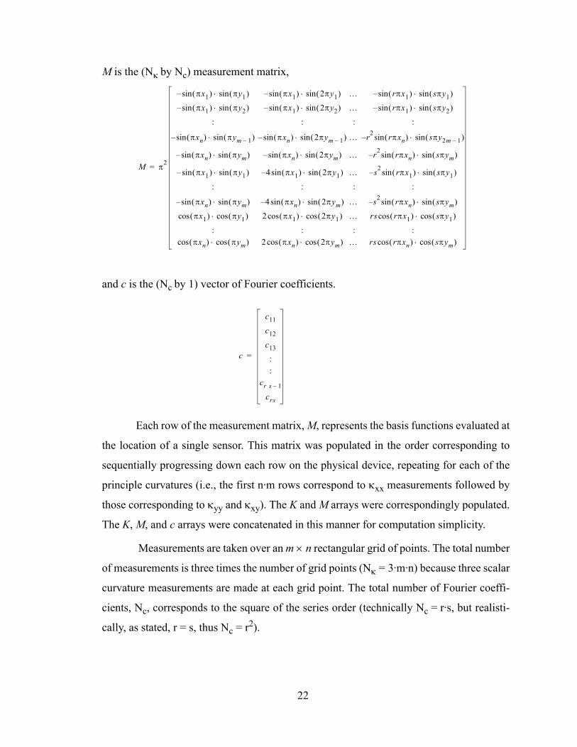
M is the (Nκ by Nc) measurement matrix,

and c is the (Nc by 1) vector of Fourier coefficients.

Each row of the measurement matrix, M, represents the basis functions evaluated at

the location of a single sensor. This matrix was populated in the order corresponding to

sequentially progressing down each row on the physical device, repeating for each of the

principle curvatures (i.e., the first n·m rows correspond to κxx measurements followed by

those corresponding to κyy and κxy). The K and M arrays were correspondingly populated.

The K, M, and c arrays were concatenated in this manner for computation simplicity.

Measurements are taken over an m × n rectangular grid of points. The total number

of measurements is three times the number of grid points (Nκ = 3·m·n) because three scalar

curvature measurements are made at each grid point. The total number of Fourier coeffi-

cients, Nc, corresponds to the square of the series order (technically Nc = r·s, but realisti-

cally, as stated, r = s, thus Nc = r2).

M π2

πx1( )sin– πy1( )sin⋅ πx1( )sin– 2πy1( )sin⋅ … rπx1( )sin– sπy1( )sin⋅

πx1( )sin– πy2( )sin⋅ πx1( )sin– 2πy2( )sin⋅ … rπx1( )sin– sπy2( )sin⋅

: : : :

πxn( )sin– πym 1–( )sin⋅ πxn( )sin– 2πym 1–( )sin⋅ … r2 rπxn( )sin– sπy2m 1–( )sin⋅

πxn( )sin– πym( )sin⋅ πxn( )sin– 2πym( )sin⋅ … r2 rπxn( )sin– sπym( )sin⋅

πx1( )sin– πy1( )sin⋅ 4 πx1( )sin– 2πy1( )sin⋅ … s2 rπx1( )sin– sπy1( )sin⋅

: : : :

πxn( )sin– πym( )sin⋅ 4 πxn( )sin– 2πym( )sin⋅ … s2 rπxn( )sin– sπym( )sin⋅

πx1( )cos πy1( )cos⋅ 2 πx1( )cos 2πy1( )cos⋅ … rs rπx1( )cos sπy1( )cos⋅

: : : :πxn( )cos πym( )cos⋅ 2 πxn( )cos 2πym( )cos⋅ … rs rπxn( )cos sπym( )cos⋅

=

c

c11

c12

c13

::

cr s 1–

crs

=

22

The standard least squares procedure gives the following estimate for the Fourier

coefficients using the Moore-Penrose left pseudo-inverse:

(3.4)

Note that since the measurement matrix, M, is dependent only on the geometry of the sensor

that the quantity can be calculated offline reducing the real time computa-

tion of Equation 3.4 to:

(3.5)

3.3 Sensor Design and ConstructionTo experimentally validate the sensor concept a simple linear array was constructed. The

linear array uses standard photoimaging and flexible circuit fabrication techniques com-

bined with standard strain gage technology. Bending strains, which are proportional to cur-

vature, are isolated using a specialized configuration of strain gages. Details of the design,

including design trades, thermal modeling, theory of operation, electronics, and construc-

tion are outlined in the following subsections.

3.3.1 Design TradesAs with any device, one must consider a complex space of design trades. The primary

trades involved the electrical, thermal, and mechanical design, which influence sensor sen-

sitivity, drift, and compliance. Informal design trades were made in order to maximize

sensor performance. The trades were not rigorous because unlike criteria that can be mod-

eled easily, performance was limited by relatively subjective constraints such as manufac-

turing risk and lead time.

Sensor performance is driven by two primary sources: resolution and membrane

compliance. Unfortunately these requirements are in direct conflict. While it is important

for the sensor to be highly sensitive, it would be useless if it did not conform to manipulated

objects. As one can see from Equation 3.14, measured signals are proportional to sensor

thickness. On the other hand, the bending stiffness is proportional to (thickness)3, so even

a small addition in sensor thickness drastically reduces its compliance. Ultimately, proto-

c MTM( )1– MT K=

MTM( )1– MT M=

c M K=

23

types were simply made as thin as possible with the commercially available prefabricated

strain gages (~175 µm and 100 µm thick, respectively for the first and second-generation

prototypes). It was also important for the sensor to be as thin as possible to prevent yielding

of the strain gages.

Another consideration in the construction of this sensor is the issue of how one

should go about measuring curvature. Strain gages were chosen as they provide a straight-

forward way to measure bending strains, which are proportional to curvature. The sensor

makes use of standard bridge circuitry, from which there are many gage configurations to

choose. Of all the possible options, a half-bridge design was chosen. The half-bridge con-

figuration (shown in Figure 3-5) reduces thermal effects and rejects axial strains, which

allows bending strains to be isolated (see Fraden [1996] and Appendix A). Both of these

properties are essential for this sensor. These characteristics are also common to full-bridge

designs; however, with the half-bridge this is accomplished with half as many active gages

and in half the amount of space. See Appendix A for more details concerning strain gage

circuitry and section 3.3.2 for further discussion of the half-bridge circuitry.

As with many sensors, it is very important to consider thermal issues in the final

sensor design, since most sensors are also thermometers. This sensor is no exception. By

utilizing a half-bridge as the sensing element, the detrimental effects of temperature fluctu-

ations are partially mitigated. However, the finite thermal resistance associated with the

polymer substrate can lead to a temperature differential between paired gages in a half-

bridge. This temperature differential creates a slight bridge imbalance that can be inter-

preted as a false curvature signal. To quantify these effects it is useful to construct a simple

thermal model of the sensor, as shown in Figures 3-3 and 3-4.

The thermal model represents a single gage-pair. The model assumes that each gage

has a uniform temperature and that its thermal capacitance is small compared to that of the

substrate and sensor skin. Rsub,X1 and Rsub,X2 represent the through-thickness thermal

resistance of the substrate for outboard and inboard gages, respectively. Rsub,Y is the ther-

mal resistance for heat dissipation into the polyimide substrate and Csub,Y is the heat capac-

ity of the polyimide substrate. Rskin,X1 represents the thermal resistance of heat flowing

from the outboard strain gage into the silicone skin. Rskin,Y is the thermal resistance for heat

24

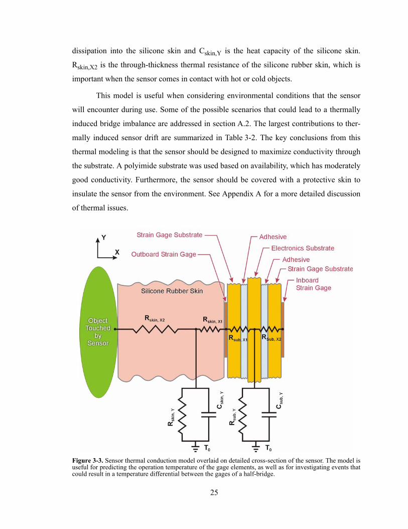
dissipation into the silicone skin and Cskin,Y is the heat capacity of the silicone skin.

Rskin,X2 is the through-thickness thermal resistance of the silicone rubber skin, which is

important when the sensor comes in contact with hot or cold objects.

This model is useful when considering environmental conditions that the sensor

will encounter during use. Some of the possible scenarios that could lead to a thermally

induced bridge imbalance are addressed in section A.2. The largest contributions to ther-

mally induced sensor drift are summarized in Table 3-2. The key conclusions from this

thermal modeling is that the sensor should be designed to maximize conductivity through

the substrate. A polyimide substrate was used based on availability, which has moderately

good conductivity. Furthermore, the sensor should be covered with a protective skin to

insulate the sensor from the environment. See Appendix A for a more detailed discussion

of thermal issues.

Figure 3-3. Sensor thermal conduction model overlaid on detailed cross-section of the sensor. The model is useful for predicting the operation temperature of the gage elements, as well as for investigating events that could result in a temperature differential between the gages of a half-bridge.

25

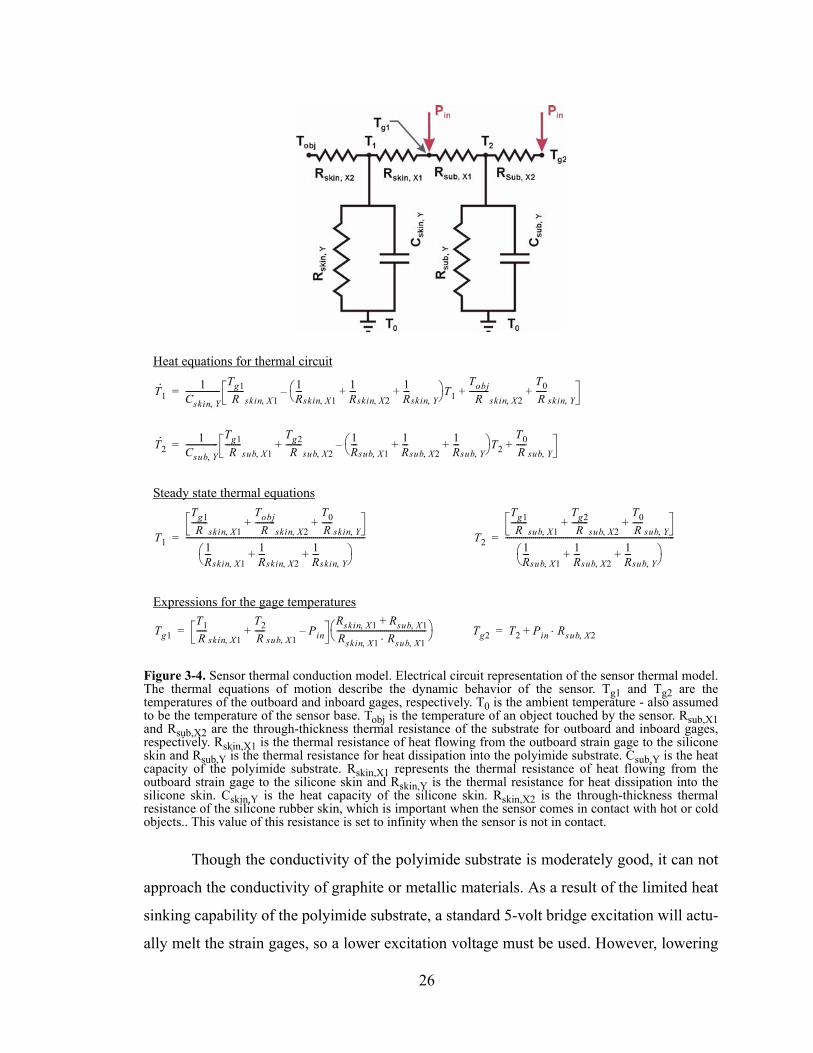
Though the conductivity of the polyimide substrate is moderately good, it can not

approach the conductivity of graphite or metallic materials. As a result of the limited heat

sinking capability of the polyimide substrate, a standard 5-volt bridge excitation will actu-

ally melt the strain gages, so a lower excitation voltage must be used. However, lowering

Figure 3-4. Sensor thermal conduction model. Electrical circuit representation of the sensor thermal model. The thermal equations of motion describe the dynamic behavior of the sensor. Tg1 and Tg2 are the temperatures of the outboard and inboard gages, respectively. T0 is the ambient temperature - also assumed to be the temperature of the sensor base. Tobj is the temperature of an object touched by the sensor. Rsub,X1and Rsub,X2 are the through-thickness thermal resistance of the substrate for outboard and inboard gages, respectively. Rskin,X1 is the thermal resistance of heat flowing from the outboard strain gage to the silicone skin and Rsub,Y is the thermal resistance for heat dissipation into the polyimide substrate. Csub,Y is the heat capacity of the polyimide substrate. Rskin,X1 represents the thermal resistance of heat flowing from the outboard strain gage to the silicone skin and Rskin,Y is the thermal resistance for heat dissipation into the silicone skin. Cskin,Y is the heat capacity of the silicone skin. Rskin,X2 is the through-thickness thermal resistance of the silicone rubber skin, which is important when the sensor comes in contact with hot or cold objects.. This value of this resistance is set to infinity when the sensor is not in contact.

Heat equations for thermal circuit

Steady state thermal equations

Expressions for the gage temperatures

T1· 1

Cskin Y,-----------------

Tg1R

--------skin X1,

1R---

skin X1,

1R---

skin X2,

1R---

skin Y,+ +

T1–Tobj

R----------

skin X2,

T0R-----

skin Y,+ +=

T2· 1

Csub Y,----------------

Tg1R

--------sub X1,

Tg2R

--------sub X2,

1R---

sub X1,

1R---

sub X2,

1R---

sub Y,+ +

T2–T0R-----

sub Y,+ +=

T1

Tg1R

--------skin X1,

TobjR

----------skin X2,

T0R-----

skin Y,+ +

1R---

skin X1,

1R---

skin X2,

1R---

skin Y,+ +

------------------------------------------------------------------------------------------= T2

Tg1R

--------sub X1,

Tg2R

--------sub X2,

T0R-----

sub Y,+ +

1R---

sub X1,

1R---

sub X2,

1R---

sub Y,+ +

-------------------------------------------------------------------------------------=

Tg1T1R-----

skin X1,

T2R-----

sub X1,Pin–+

Rskin X1, Rsub X1,+Rskin X1, Rsub X1,⋅---------------------------------------------

= Tg2 T2 Pin Rsub X2,⋅+=

26

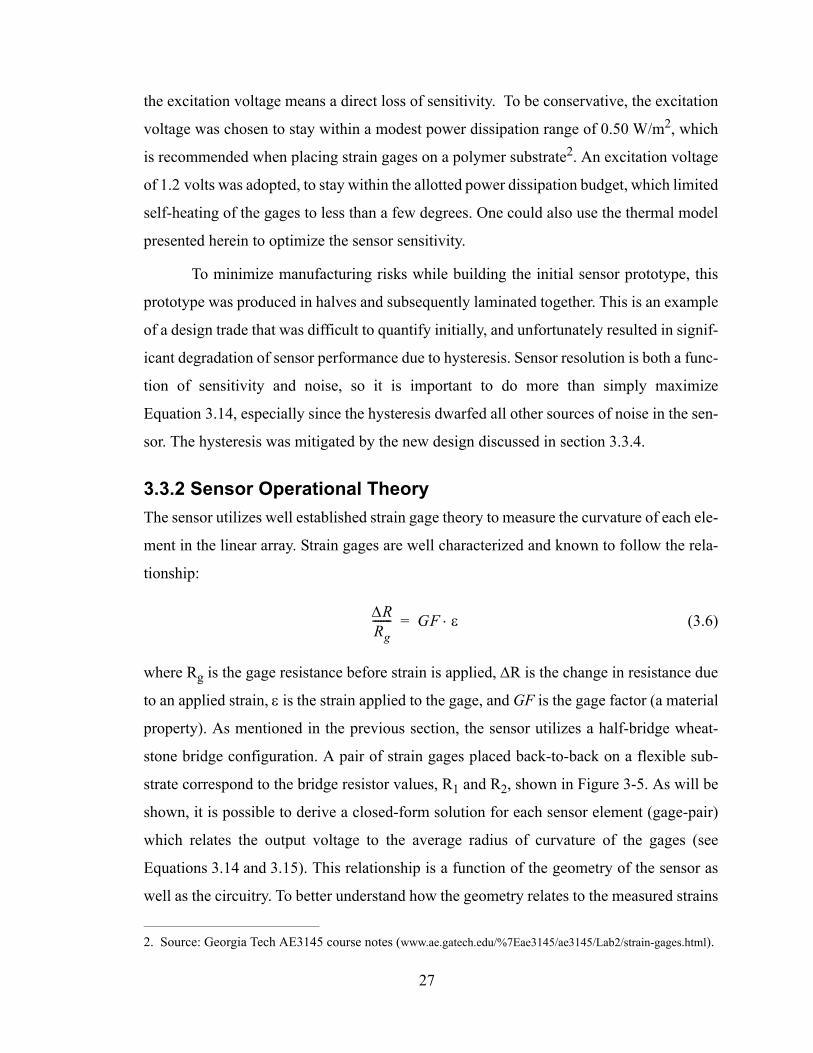
the excitation voltage means a direct loss of sensitivity. To be conservative, the excitation

voltage was chosen to stay within a modest power dissipation range of 0.50 W/m2, which

is recommended when placing strain gages on a polymer substrate2. An excitation voltage

of 1.2 volts was adopted, to stay within the allotted power dissipation budget, which limited

self-heating of the gages to less than a few degrees. One could also use the thermal model

presented herein to optimize the sensor sensitivity.

To minimize manufacturing risks while building the initial sensor prototype, this

prototype was produced in halves and subsequently laminated together. This is an example

of a design trade that was difficult to quantify initially, and unfortunately resulted in signif-

icant degradation of sensor performance due to hysteresis. Sensor resolution is both a func-

tion of sensitivity and noise, so it is important to do more than simply maximize

Equation 3.14, especially since the hysteresis dwarfed all other sources of noise in the sen-

sor. The hysteresis was mitigated by the new design discussed in section 3.3.4.

3.3.2 Sensor Operational TheoryThe sensor utilizes well established strain gage theory to measure the curvature of each ele-

ment in the linear array. Strain gages are well characterized and known to follow the rela-

tionship:

(3.6)

where Rg is the gage resistance before strain is applied, ∆R is the change in resistance due

to an applied strain, ε is the strain applied to the gage, and GF is the gage factor (a material

property). As mentioned in the previous section, the sensor utilizes a half-bridge wheat-

stone bridge configuration. A pair of strain gages placed back-to-back on a flexible sub-

strate correspond to the bridge resistor values, R1 and R2, shown in Figure 3-5. As will be

shown, it is possible to derive a closed-form solution for each sensor element (gage-pair)

which relates the output voltage to the average radius of curvature of the gages (see

Equations 3.14 and 3.15). This relationship is a function of the geometry of the sensor as

well as the circuitry. To better understand how the geometry relates to the measured strains

2. Source: Georgia Tech AE3145 course notes (www.ae.gatech.edu/%7Eae3145/ae3145/Lab2/strain-gages.html).

∆RRg------- GF ε⋅=

27

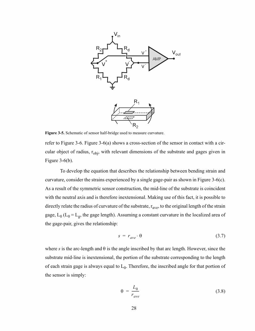
refer to Figure 3-6. Figure 3-6(a) shows a cross-section of the sensor in contact with a cir-

cular object of radius, robj, with relevant dimensions of the substrate and gages given in

Figure 3-6(b).

To develop the equation that describes the relationship between bending strain and

curvature, consider the strains experienced by a single gage-pair as shown in Figure 3-6(c).

As a result of the symmetric sensor construction, the mid-line of the substrate is coincident

with the neutral axis and is therefore inextensional. Making use of this fact, it is possible to

directly relate the radius of curvature of the substrate, rave, to the original length of the strain

gage, L0 (L0 = Lg, the gage length). Assuming a constant curvature in the localized area of

the gage-pair, gives the relationship:

(3.7)

where s is the arc-length and θ is the angle inscribed by that arc length. However, since the

substrate mid-line is inextensional, the portion of the substrate corresponding to the length

of each strain gage is always equal to L0. Therefore, the inscribed angle for that portion of

the sensor is simply:

(3.8)

Figure 3-5. Schematic of sensor half-bridge used to measure curvature.

s rave θ⋅=

θL0

rave---------=

28

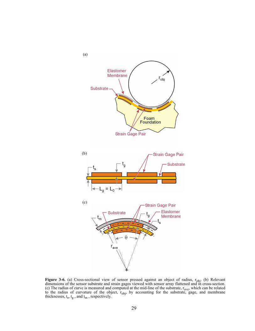
Figure 3-6. (a) Cross-sectional view of sensor pressed against an object of radius, robj. (b) Relevant dimensions of the sensor substrate and strain gages viewed with sensor array flattened and in cross-section. (c) The radius of curve is measured and computed at the mid-line of the substrate, rave, which can be related to the radius of curvature of the object, robj, by accounting for the substrate, gage, and membrane thicknesses, ts, tg , and tm , respectively.

(a)

(b)

(c)

29

A modified version of Equation 3.7 can also be used to express the current length,

L, of the mid-line of the upper strain gage (in tension), by making a small correction to the

radius:

(3.9)

where tg and ts are the gage and substrate thicknesses, respectively. Combining

Equations 3.8 and 3.9, gives a formula for the current gage length expressed in terms of a

single unknown, rave.

(3.10)

The length of the bottom strain gage can be calculated in a similar fashion.

The next step is to compute the strain experienced by the strain gages. The formula

for the engineering strain is:

(3.11)

As expressed earlier, L and L0 are the current and undeformed lengths of a strain gage ele-

ment, respectively. Substituting the result from Equation 3.10 into Equation 3.11, gives the

strain in the upper strain gage, expressed as a function of the substrate radius.

(3.12)

The strain in the bottom strain gage is equal and opposite to that shown in Equation 3.12

(from sensor symmetry). Solving for the change in resistance which accompanies bending

induced strain is now simply a matter of combining Equations 3.6 and 3.12.

(3.13)

L ravets tg+

2--------------+

θ⋅=

L ravets tg+

2--------------+

L0rave---------⋅=

εL L0–

L0---------------=

εrave

ts tg+2

--------------+ L0

rave---------⋅ L0–

L0-------------------------------------------------------------

ts tg+2 rave--------------= =

∆RRg GF ts tg+( )

2 rave-------------------------------------=

30

Substituting Equation 3.13 into a standard wheatstone bridge formulation (see

Appendix A: Equations A.3 and A.4) yields the final bridge equation for measuring bend-

ing strains with a pair of back-to-back gages wired in a half-bridge configuration (as shown

in Figure 3-5).

(3.14)

where Vin is the bridge excitation voltage, rave is the curvature of the membrane centerline,

ts is the thickness of the membrane substrate, tg is the gage thickness and “Gain” is the

bridge amplification. Equation 3.14 can be rearranged in terms of average curvature, κ,

where curvature can be shown as the reciprocal of radius of curvature and κ(i) represents

the curvature of the ith gage-pair.

(3.15)

The sensor was designed to stay within the elastic limits of the metal foil strain

gages (about 1% strain for constantan alloy).

VoutVin GF ts tg+( ) Gain⋅ ⋅⋅

4rave-------------------------------------------------------------=

κ i( ) 1rave---------=

4VoutVin GF ts tg+( ) Gain⋅ ⋅⋅-------------------------------------------------------------=

31

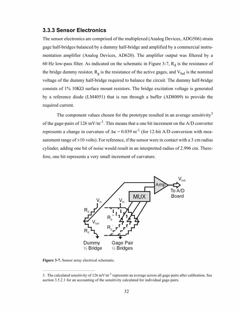
3.3.3 Sensor ElectronicsThe sensor electronics are comprised of the multiplexed (Analog Devices, ADG506) strain

gage half-bridges balanced by a dummy half-bridge and amplified by a commercial instru-

mentation amplifier (Analog Devices, AD620). The amplifier output was filtered by a

60 Hz low-pass filter. As indicated on the schematic in Figure 3-7, Rd is the resistance of

the bridge dummy resistor, Rg is the resistance of the active gages, and Vbal is the nominal

voltage of the dummy half-bridge required to balance the circuit. The dummy half-bridge

consists of 1% 10KΩ surface mount resistors. The bridge excitation voltage is generated

by a reference diode (LM4051) that is run through a buffer (AD8009) to provide the

required current.

The component values chosen for the prototype resulted in an average sensitivity3

of the gage-pairs of 126 mV/m-1. This means that a one bit increment on the A/D converter

represents a change in curvature of ∆κ = 0.039 m-1 (for 12-bit A/D conversion with mea-

surement range of ±10 volts). For reference, if the sensor were in contact with a 3 cm radius

cylinder, adding one bit of noise would result in an interpretted radius of 2.996 cm. There-

fore, one bit represents a very small increment of curvature.

3. The calculated sensitivity of 126 mV/m-1 represents an average across all gage-pairs after calibration. See section 3.5.2.1 for an accounting of the sensitivity calculated for individual gage-pairs.

Figure 3-7. Sensor array electrical schematic.

32

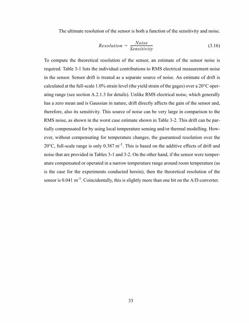
The ultimate resolution of the sensor is both a function of the sensitivity and noise.

(3.16)

To compute the theoretical resolution of the sensor, an estimate of the sensor noise is

required. Table 3-1 lists the individual contributions to RMS electrical measurement noise

in the sensor. Sensor drift is treated as a separate source of noise. An estimate of drift is

calculated at the full-scale 1.0% strain level (the yield strain of the gages) over a 20°C oper-

ating range (see section A.2.1.3 for details). Unlike RMS electrical noise, which generally

has a zero mean and is Gaussian in nature, drift directly affects the gain of the sensor and,

therefore, also its sensitivity. This source of noise can be very large in comparison to the

RMS noise, as shown in the worst case estimate shown in Table 3-2. This drift can be par-

tially compensated for by using local temperature sensing and/or thermal modelling. How-

ever, without compensating for temperature changes, the guaranteed resolution over the

20°C, full-scale range is only 0.387 m-1. This is based on the additive effects of drift and

noise that are provided in Tables 3-1 and 3-2. On the other hand, if the sensor were temper-

ature compensated or operated in a narrow temperature range around room temperature (as

is the case for the experiments conducted herein), then the theoretical resolution of the

sensor is 0.041 m-1. Coincidentally, this is slightly more than one bit on the A/D converter.

Resolution NoiseSensitivity----------------------------=

33

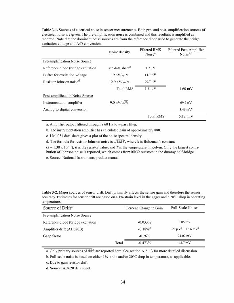
Table 3-1. Sources of electrical noise in sensor measurements. Both pre- and post- amplification sources of electrical noise are given. The pre-amplification noise is combined and this resultant is amplified as reported. Note that the dominant noise sources are from the reference diode used to generate the bridge excitation voltage and A/D conversion.

Noise density Filtered RMS Noisea

a. Amplifier output filtered through a 60 Hz low-pass filter.

Filtered Post-Amplifier Noisea,b

b. The instrumentation amplifier has calculated gain of approximately 880.

Pre-amplification Noise Source

Reference diode (bridge excitation) see data sheetc

c. LM4051 data sheet gives a plot of the noise spectral density

1.7 µV

Buffer for excitation voltage 1.9 nV/ 14.7 nV

Resistor Johnson noised

d. The formula for resistor Johnson noise is , where k is Boltzman’s constant (k = 1.38 x 10-23), R is the resistor value, and T is the temperature in Kelvin. Only the largest contri-bution of Johnson noise is reported, which comes from10KΩ resistors in the dummy half-bridge.

12.9 nV/ 99.7 nV

Total RMS 1.81 µV 1.60 mV

Post-amplification Noise Source

Instrumentation amplifier 9.0 nV/ 69.7 nV

Analog-to-digital conversion 3.46 mVe

Total RMS 5.12 ,mV

e. Source: National Instruments product manual

Hz

4kRT

Hz

Hz

Table 3-2. Major sources of sensor drift. Drift primarily affects the sensor gain and therefore the sensor accuracy. Estimates for sensor drift are based on a 1% strain level in the gages and a 20°C drop in operating temperature.

Source of Drifta

a. Only primary sources of drift are reported here. See section A.2.1.3 for more detailed discussion.

Percent Change in Gain Full-Scale Noiseb

b. Full-scale noise is based on either 1% strain and/or 20°C drop in temperature, as applicable.

Pre-amplification Noise Source

Reference diode (bridge excitation) -0.033% 3.05 mV

Amplifier drift (AD620B) -0.18%c

c. Due to gain resistor drift

~20 µVd + 16.6 mVc

Gage factor -0.26% 24.02 mV

Total -0.473% 43.7 mV

d. Source: AD620 data sheet.

34

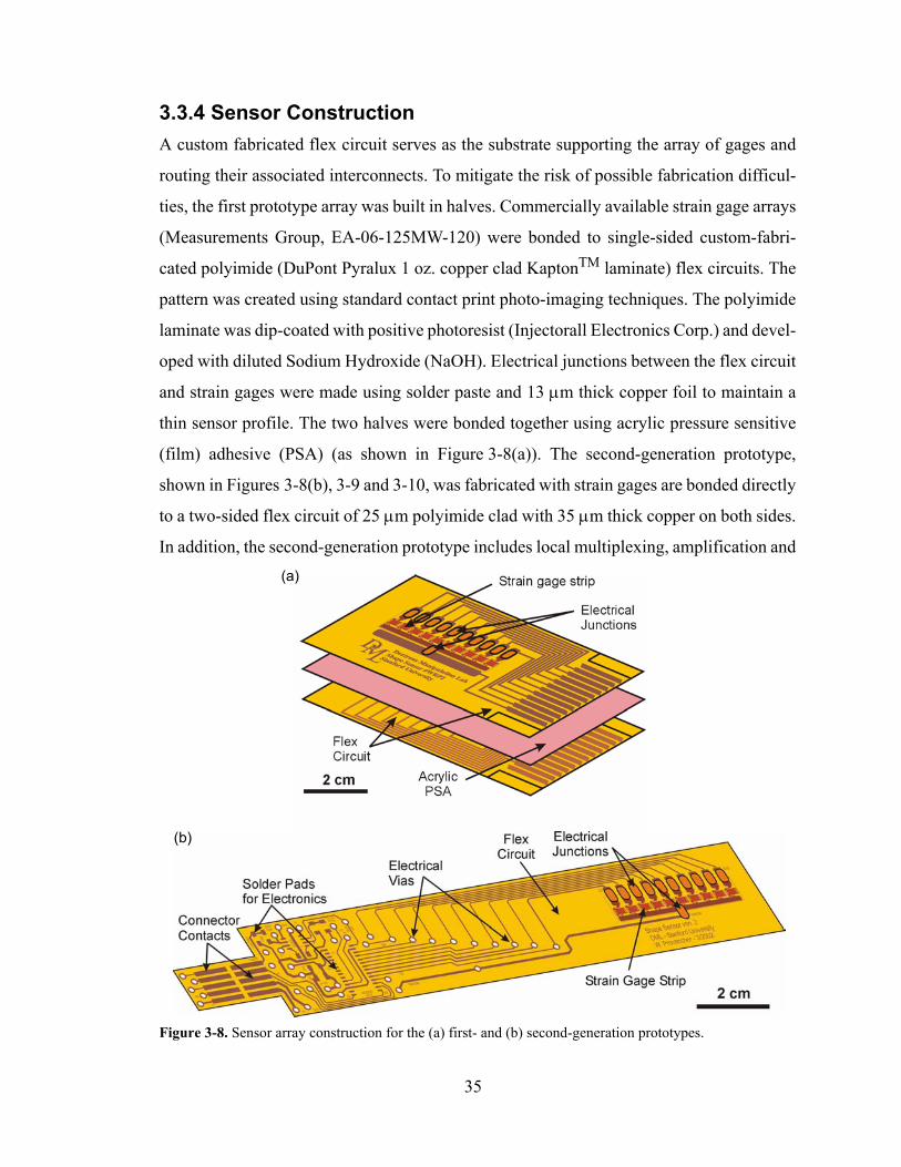
3.3.4 Sensor ConstructionA custom fabricated flex circuit serves as the substrate supporting the array of gages and

routing their associated interconnects. To mitigate the risk of possible fabrication difficul-

ties, the first prototype array was built in halves. Commercially available strain gage arrays

(Measurements Group, EA-06-125MW-120) were bonded to single-sided custom-fabri-

cated polyimide (DuPont Pyralux 1 oz. copper clad KaptonTM laminate) flex circuits. The

pattern was created using standard contact print photo-imaging techniques. The polyimide

laminate was dip-coated with positive photoresist (Injectorall Electronics Corp.) and devel-

oped with diluted Sodium Hydroxide (NaOH). Electrical junctions between the flex circuit

and strain gages were made using solder paste and 13 µm thick copper foil to maintain a

thin sensor profile. The two halves were bonded together using acrylic pressure sensitive

(film) adhesive (PSA) (as shown in Figure 3-8(a)). The second-generation prototype,

shown in Figures 3-8(b), 3-9 and 3-10, was fabricated with strain gages are bonded directly

to a two-sided flex circuit of 25 µm polyimide clad with 35 µm thick copper on both sides.

In addition, the second-generation prototype includes local multiplexing, amplification and

Figure 3-8. Sensor array construction for the (a) first- and (b) second-generation prototypes.

(a)

(b)

35

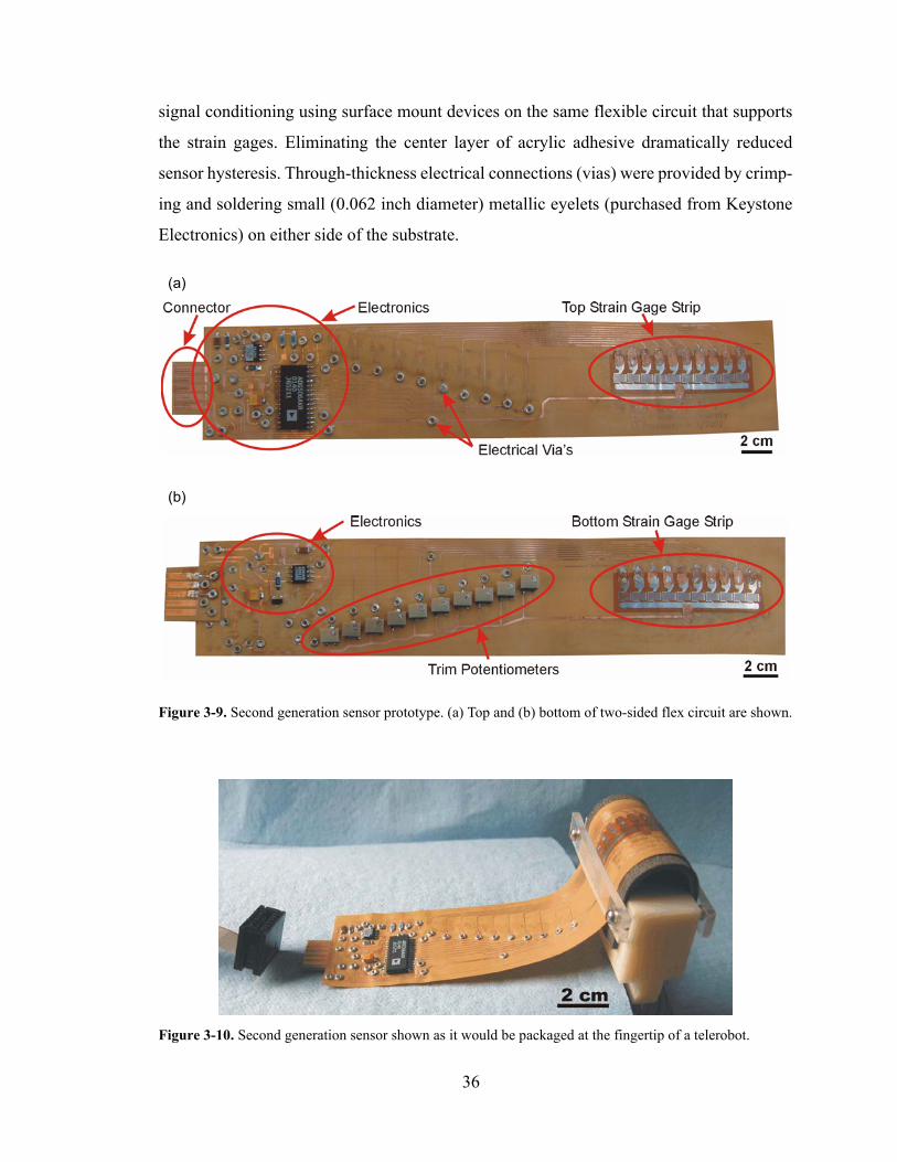
signal conditioning using surface mount devices on the same flexible circuit that supports

the strain gages. Eliminating the center layer of acrylic adhesive dramatically reduced

sensor hysteresis. Through-thickness electrical connections (vias) were provided by crimp-

ing and soldering small (0.062 inch diameter) metallic eyelets (purchased from Keystone

Electronics) on either side of the substrate.

Figure 3-9. Second generation sensor prototype. (a) Top and (b) bottom of two-sided flex circuit are shown.

(a)

(b)

Figure 3-10. Second generation sensor shown as it would be packaged at the fingertip of a telerobot.

36

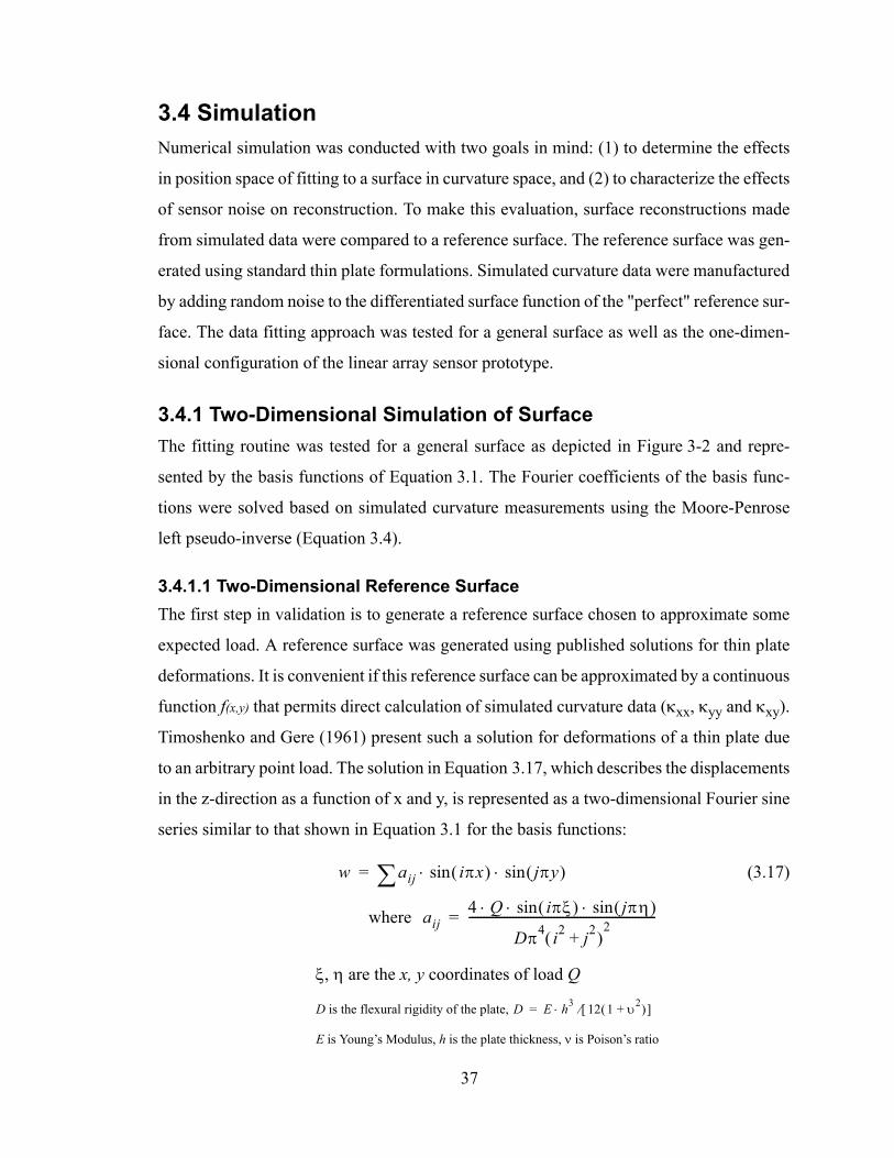
3.4 SimulationNumerical simulation was conducted with two goals in mind: (1) to determine the effects

in position space of fitting to a surface in curvature space, and (2) to characterize the effects

of sensor noise on reconstruction. To make this evaluation, surface reconstructions made

from simulated data were compared to a reference surface. The reference surface was gen-

erated using standard thin plate formulations. Simulated curvature data were manufactured

by adding random noise to the differentiated surface function of the "perfect" reference sur-

face. The data fitting approach was tested for a general surface as well as the one-dimen-

sional configuration of the linear array sensor prototype.

3.4.1 Two-Dimensional Simulation of SurfaceThe fitting routine was tested for a general surface as depicted in Figure 3-2 and repre-

sented by the basis functions of Equation 3.1. The Fourier coefficients of the basis func-

tions were solved based on simulated curvature measurements using the Moore-Penrose

left pseudo-inverse (Equation 3.4).

3.4.1.1 Two-Dimensional Reference SurfaceThe first step in validation is to generate a reference surface chosen to approximate some

expected load. A reference surface was generated using published solutions for thin plate

deformations. It is convenient if this reference surface can be approximated by a continuous

function f(x,y) that permits direct calculation of simulated curvature data (κxx, κyy and κxy).

Timoshenko and Gere (1961) present such a solution for deformations of a thin plate due

to an arbitrary point load. The solution in Equation 3.17, which describes the displacements

in the z-direction as a function of x and y, is represented as a two-dimensional Fourier sine

series similar to that shown in Equation 3.1 for the basis functions:

(3.17)

where

ξ, η are the x, y coordinates of load Q

D is the flexural rigidity of the plate,

E is Young’s Modulus, h is the plate thickness, ν is Poison’s ratio

w aij iπx( ) jπy( )sin⋅sin⋅∑=

aij4 Q iπξ( ) jπη( )sin⋅sin⋅ ⋅

Dπ4 i2 j2+( )2

----------------------------------------------------------------=

D E h3 12 1 υ2+( )[ ]⁄⋅=

37

More complex load cases can be represented through superposition of several point loads.

For simulation, three load cases were considered: (1) a centered point load (ξ = 0.5,

η = 0.5), (2) an off-center point load (ξ = 0.2, η = 0.8), and (3) a skewed line load (from

ξ = 0.1, η = 0.9 to ξ = 0.9, η = 0.1). Simulated curvature data were produced by taking

appropriate derivatives of the reference surface displacement function. To simulate the

effects of sensor noise on the reconstruction, random noise, with RMS value of

∆κ = 0.23 m-1 (approximately 25% of the average curvature values) and a maximum value

of ∆κ = 0.40 m-1, was added to the simulated curvature data. The basis functions were fit

directly to the simulated curvature data. The “truth” model for the two-dimensional surface

was represented by a two-dimensional (15 × 15) Fourier series. There were 100 measure-

ment points (10 × 10) with three measurements at each point for a total of 300 measure-

ments. The fitted model had 64 parameters (8 × 8) Fourier coefficients. An eighth order

series was chosen because it is a realistic size for real time computation.

3.4.1.2 Two-Dimensional Simulation ResultsThe quality of data fitting was quantified by recording the maximum calculated displace-

ment, wMax, at the point of load application and the distributed RMS error, Ew,RMS, relative

to the reference surface. The first metric was chosen because of its significance to manip-

ulation kinematics. During manipulation, the point of load application is the same as the

object contact point and small deformations at the robot fingertip ultimately affect the pre-

cision of fine manipulations. Table 3-3 reports the maximum calculated displacement at the

point of load application, wMax, the absolute error of this displacement, Ew,Max, and the

RMS error for the entire surface, Ew,RMS, as compared to the reference surface. Figure 3-11

shows mesh plots of two-dimensional simulation results.

38

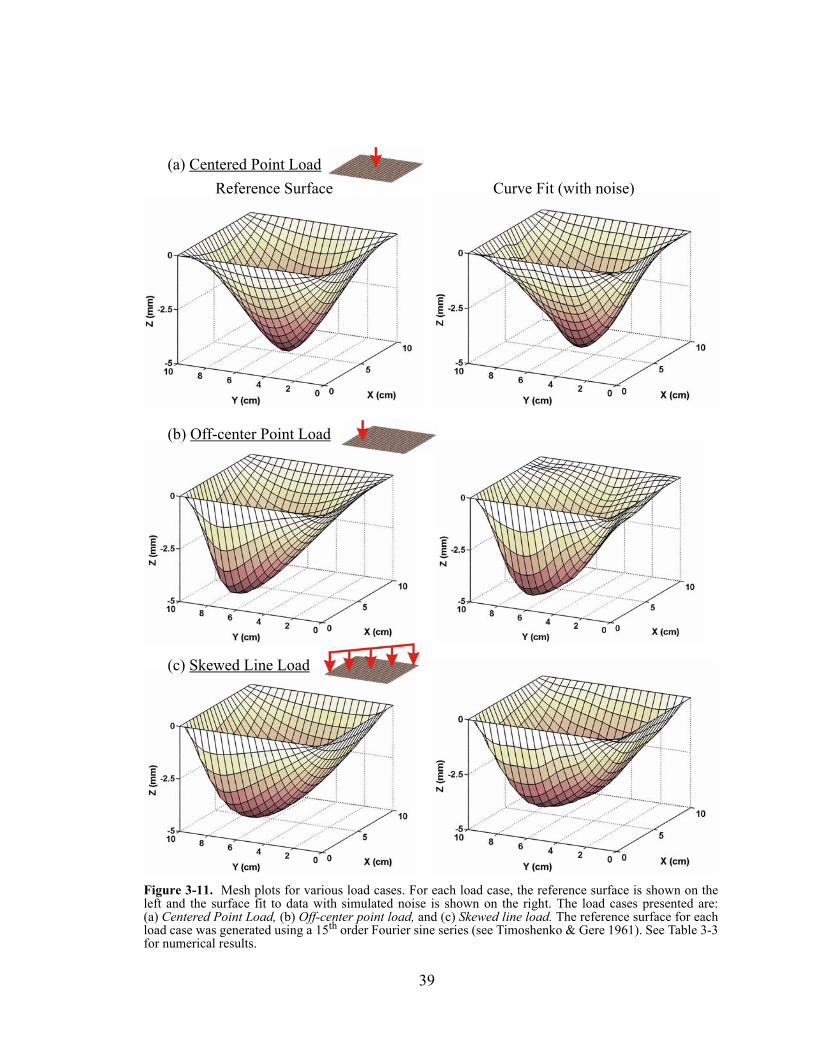
Figure 3-11. Mesh plots for various load cases. For each load case, the reference surface is shown on the left and the surface fit to data with simulated noise is shown on the right. The load cases presented are: (a) Centered Point Load, (b) Off-center point load, and (c) Skewed line load. The reference surface for each load case was generated using a 15th order Fourier sine series (see Timoshenko & Gere 1961). See Table 3-3for numerical results.

(a) Centered Point Load

(b) Off-center Point Load

(c) Skewed Line Load

Reference Surface Curve Fit (with noise)

39

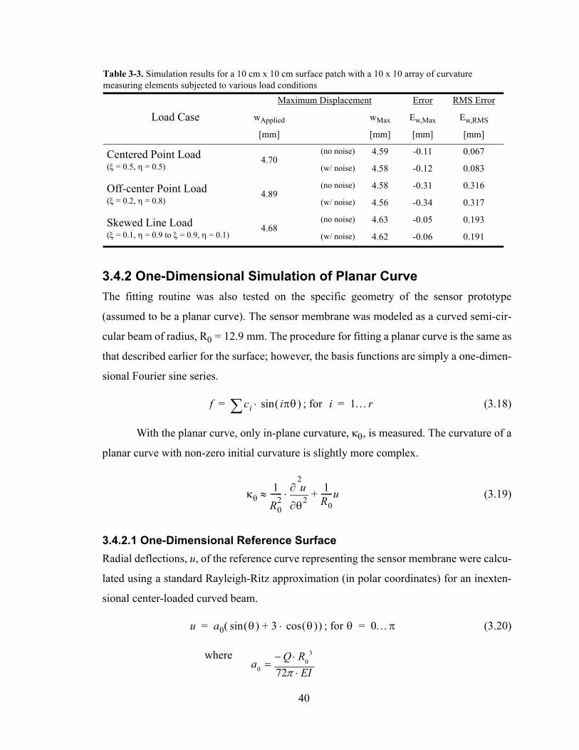
3.4.2 One-Dimensional Simulation of Planar CurveThe fitting routine was also tested on the specific geometry of the sensor prototype

(assumed to be a planar curve). The sensor membrane was modeled as a curved semi-cir-

cular beam of radius, R0 = 12.9 mm. The procedure for fitting a planar curve is the same as

that described earlier for the surface; however, the basis functions are simply a one-dimen-

sional Fourier sine series.

; for (3.18)

With the planar curve, only in-plane curvature, κθ, is measured. The curvature of a

planar curve with non-zero initial curvature is slightly more complex.

(3.19)

3.4.2.1 One-Dimensional Reference SurfaceRadial deflections, u, of the reference curve representing the sensor membrane were calcu-

lated using a standard Rayleigh-Ritz approximation (in polar coordinates) for an inexten-

sional center-loaded curved beam.

; for (3.20)

where

Table 3-3. Simulation results for a 10 cm x 10 cm surface patch with a 10 x 10 array of curvature measuring elements subjected to various load conditions

Load CaseMaximum Displacement Error RMS Error

wApplied wMax Ew,Max Ew,RMS

[mm] [mm] [mm] [mm]

Centered Point Load(ξ = 0.5, η = 0.5)

4.70(no noise) 4.59 -0.11 0.067

(w/ noise) 4.58 -0.12 0.083

Off-center Point Load(ξ = 0.2, η = 0.8)

4.89(no noise) 4.58 -0.31 0.316

(w/ noise) 4.56 -0.34 0.317

Skewed Line Load(ξ = 0.1, η = 0.9 to ξ = 0.9, η = 0.1)

4.68(no noise) 4.63 -0.05 0.193

(w/ noise) 4.62 -0.06 0.191

f ci iπθ( )sin⋅∑= i 1…r=

κθ1

R02

------θ2

2

∂

∂ u⋅ 1R0------u+≈

u a0 θ( ) 3 θ( )cos⋅+sin( )= θ 0…π=

EIRQ

a⋅⋅−

=π72

30

0

40

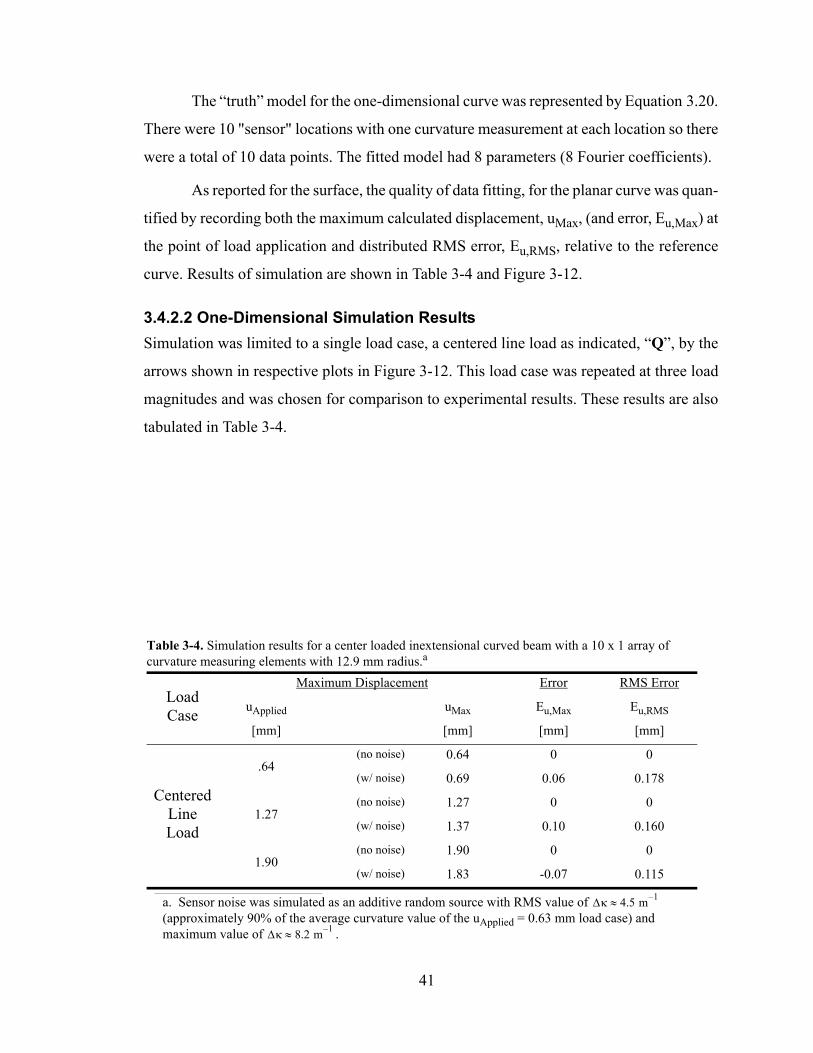
The “truth” model for the one-dimensional curve was represented by Equation 3.20.

There were 10 "sensor" locations with one curvature measurement at each location so there

were a total of 10 data points. The fitted model had 8 parameters (8 Fourier coefficients).

As reported for the surface, the quality of data fitting, for the planar curve was quan-

tified by recording both the maximum calculated displacement, uMax, (and error, Eu,Max) at

the point of load application and distributed RMS error, Eu,RMS, relative to the reference

curve. Results of simulation are shown in Table 3-4 and Figure 3-12.

3.4.2.2 One-Dimensional Simulation ResultsSimulation was limited to a single load case, a centered line load as indicated, “Q”, by the

arrows shown in respective plots in Figure 3-12. This load case was repeated at three load

magnitudes and was chosen for comparison to experimental results. These results are also

tabulated in Table 3-4.

Table 3-4. Simulation results for a center loaded inextensional curved beam with a 10 x 1 array of curvature measuring elements with 12.9 mm radius.a

a. Sensor noise was simulated as an additive random source with RMS value of (approximately 90% of the average curvature value of the uApplied = 0.63 mm load case) and maximum value of .

Load Case

Maximum Displacement Error RMS Error

uApplied uMax Eu,Max Eu,RMS

[mm] [mm] [mm] [mm]

Centered Line Load

.64(no noise) 0.64 0 0

(w/ noise) 0.69 0.06 0.178

1.27(no noise) 1.27 0 0

(w/ noise) 1.37 0.10 0.160

1.90(no noise) 1.90 0 0

(w/ noise) 1.83 -0.07 0.115

∆κ 4.5 m 1–≈

∆κ 8.2 m 1–≈

41

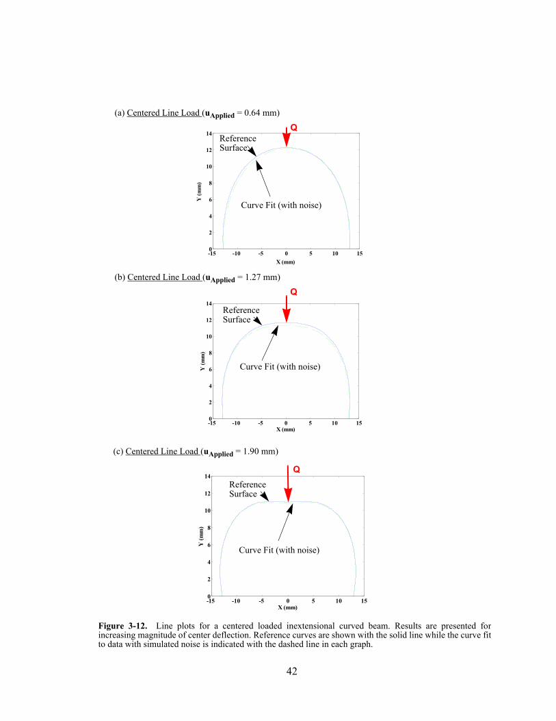
Figure 3-12. Line plots for a centered loaded inextensional curved beam. Results are presented for increasing magnitude of center deflection. Reference curves are shown with the solid line while the curve fit to data with simulated noise is indicated with the dashed line in each graph.

(b) Centered Line Load (uApplied = 1.27 mm)

(c) Centered Line Load (uApplied = 1.90 mm)

-15 -10 -5 0 5 10 150

2

4

6

8

10

12

14

X (mm)

Y (m

m)

Rayleigh-Ritz Data Curve Fit (with Noise)

-15 -10 -5 0 5 10 150

2

4

6

8

10

12

14

X (mm)

Y (m

m)

-15 -10 -5 0 5 10 150

2

4

6

8

10

12

14

X (mm)

Y (m

m)

Curve Fit (with noise)

Reference

Curve Fit (with noise)

Reference

Q

Q

Q

Surface

Surface

ReferenceSurface

Curve Fit (with noise)

(a) Centered Line Load (uApplied = 0.64 mm)

42

3.4.3 Discussion of Simulation ResultsThe numerical simulation results show that a series of discrete curvature measurements can

be used to create a reasonably accurate reconstruction of the deformed membrane. When

moderate levels of noise are added, the maximum position error increases to as much as

10% for moderate deflections. Since it is difficult to predict the RMS noise of actual sensor

data without extensive characterization, random noise was introduced to the simulation at

the same order of magnitude as the widest “hysteresis gap” presented in Figure 3-13, in the

next section. The accuracy of the surface reconstruction improves and the sensitivity to

sensor noise rapidly decreases as the number of sensors increases. Of course, increasing the

number of sensors also increases the difficulty in manufacturing and the computation time.

3.5 Experimental ValidationThis section presents results of the sensor calibration and testing. The following sub-sec-

tions present the experimental procedure and a discussion of the results.

3.5.1 Experimental Procedure

3.5.1.1 Calibration and Hysteresis TestingTo confirm proper sensor operation before embedding in a robot fingertip, the sensor was

calibrated against cylindrical objects of known curvature. One would expect the sensor

output to be directly proportional to object curvature. This was confirmed for objects with

small curvature.

Testing of a first-generation sensor revealed hysteresis, which was traced to creep

in the acrylic film adhesive. To quantify the hysteresis, measurements were made against a

sequence of objects of known curvature, as shown in Figure 3-13(a). Data were recorded

starting with objects of large radius of curvature (small curvature) and progressing to

objects of decreasing radius of curvature and back again to objects of larger radius of cur-

vature. The sensor was then flipped over and measurements of objects were made with the

opposite face of the sensor in contact with the objects, again starting with large objects and

progressing as described above. This procedure was carried out to form one complete hys-

teresis loop. Each gage-pair of the sensor was calibrated over the range of measurements

43

taken during the above procedure. Calibration consisted of standard least-squares fitting of

curvature data.

3.5.1.2 Centered Line Load TestA simple test configuration was chosen to validate the sensor concept experimentally. The

sensor was tested as it would be used on a cylindrical robot fingertip (Figure 3-10). A cen-

tered line load was applied to the sensor, indicated as “Q” in Figure 3-14. For this type of

loading, the sensor deforms as a curved beam of radius, R0 = 12.9 mm.

For practicality, instead of applying a line load, a known line-deflection was applied

to the center of the sensor using a height gauge. The applied center deflection, uMax, of the

sensor was recorded for three discrete load cases of increasing magnitude

(uApplied = 0.64 mm, 1.27 mm and 1.90 mm). Only one measurement per gage-pair was

taken during testing. These discrete curvature signals were utilized to reconstructed the

deformed shape of the sensor, as described previously. The quality of data fitting for the

experiments was quantified by comparing the maximum calculated displacement, uMax, at

the point of load application with the applied deflection. The reconstructed sensor shape is

also compared to the shape expected from standard solutions. There were ten curvature

measurements, one at each of ten data points.

3.5.2 Experimental Results and Discussion

3.5.2.1 Calibration and Hysteresis TestingThe second-generation prototype (shown in Figures 3-9 and 3-10) was characterized and

calibrated as described in section 3.5.1.1. Data were recorded at each gage-pair at each step

through the calibration procedure. Sensor data were collected to complete one hysteresis

loop. The second generation of the shape sensor represents a three-fold improvement over

the first generation design, though significant hysteresis persists (as shown in Figure 3-13).

Figure 3-13(a) shows data for each gage-pair on the sensor in a different color. Note

that there are slight variations between the behavior of individual gage-pairs; however, they

all bear resemblance to one another, having similar slope and shape. Figure 3-13(b) shows

calibration from a single gage-pair, while Figure 3-13(c) shows calibration data averaged

across all gage-pairs in the sensor. Both of these graphs show the formation of a small hys-

44

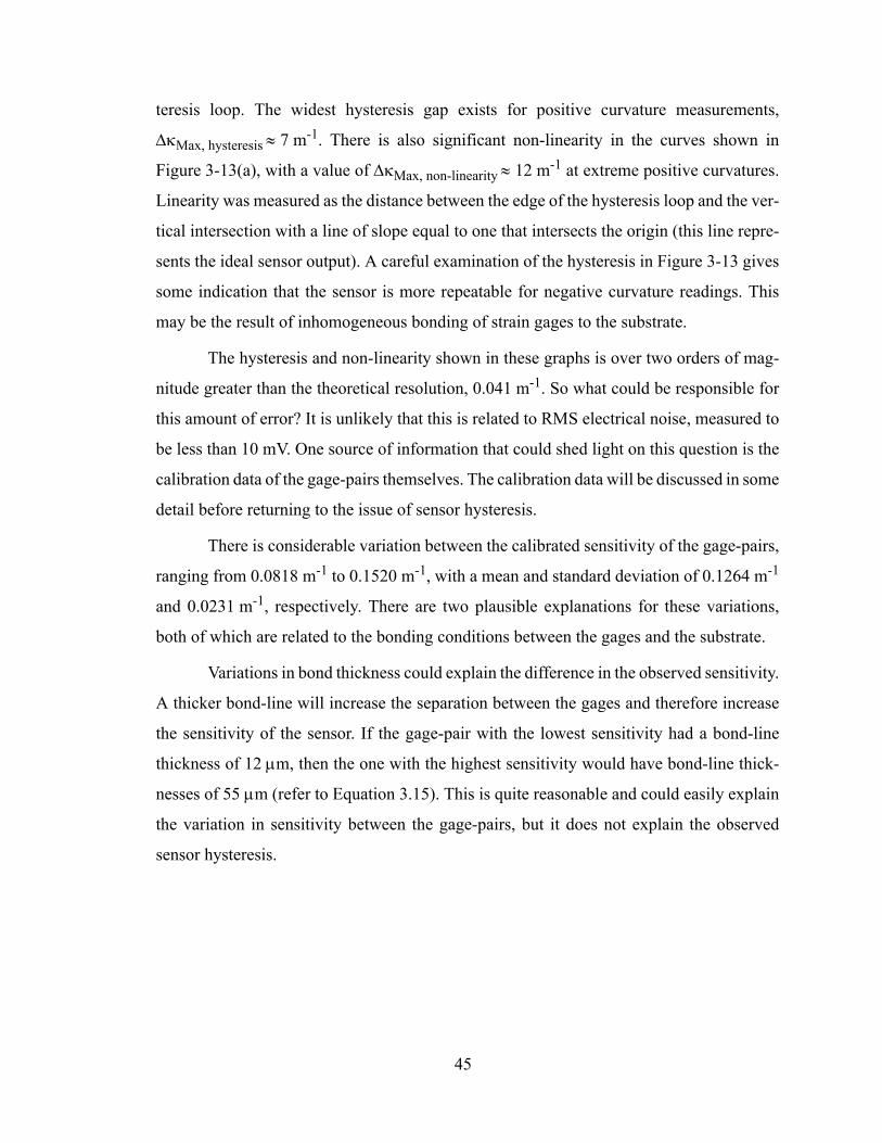
teresis loop. The widest hysteresis gap exists for positive curvature measurements,

∆κMax, hysteresis ≈ 7 m-1. There is also significant non-linearity in the curves shown in

Figure 3-13(a), with a value of ∆κMax, non-linearity ≈ 12 m-1 at extreme positive curvatures.

Linearity was measured as the distance between the edge of the hysteresis loop and the ver-

tical intersection with a line of slope equal to one that intersects the origin (this line repre-

sents the ideal sensor output). A careful examination of the hysteresis in Figure 3-13 gives

some indication that the sensor is more repeatable for negative curvature readings. This

may be the result of inhomogeneous bonding of strain gages to the substrate.

The hysteresis and non-linearity shown in these graphs is over two orders of mag-

nitude greater than the theoretical resolution, 0.041 m-1. So what could be responsible for

this amount of error? It is unlikely that this is related to RMS electrical noise, measured to

be less than 10 mV. One source of information that could shed light on this question is the

calibration data of the gage-pairs themselves. The calibration data will be discussed in some

detail before returning to the issue of sensor hysteresis.

There is considerable variation between the calibrated sensitivity of the gage-pairs,

ranging from 0.0818 m-1 to 0.1520 m-1, with a mean and standard deviation of 0.1264 m-1

and 0.0231 m-1, respectively. There are two plausible explanations for these variations,

both of which are related to the bonding conditions between the gages and the substrate.

Variations in bond thickness could explain the difference in the observed sensitivity.

A thicker bond-line will increase the separation between the gages and therefore increase

the sensitivity of the sensor. If the gage-pair with the lowest sensitivity had a bond-line

thickness of 12 µm, then the one with the highest sensitivity would have bond-line thick-

nesses of 55 µm (refer to Equation 3.15). This is quite reasonable and could easily explain

the variation in sensitivity between the gage-pairs, but it does not explain the observed

sensor hysteresis.

45

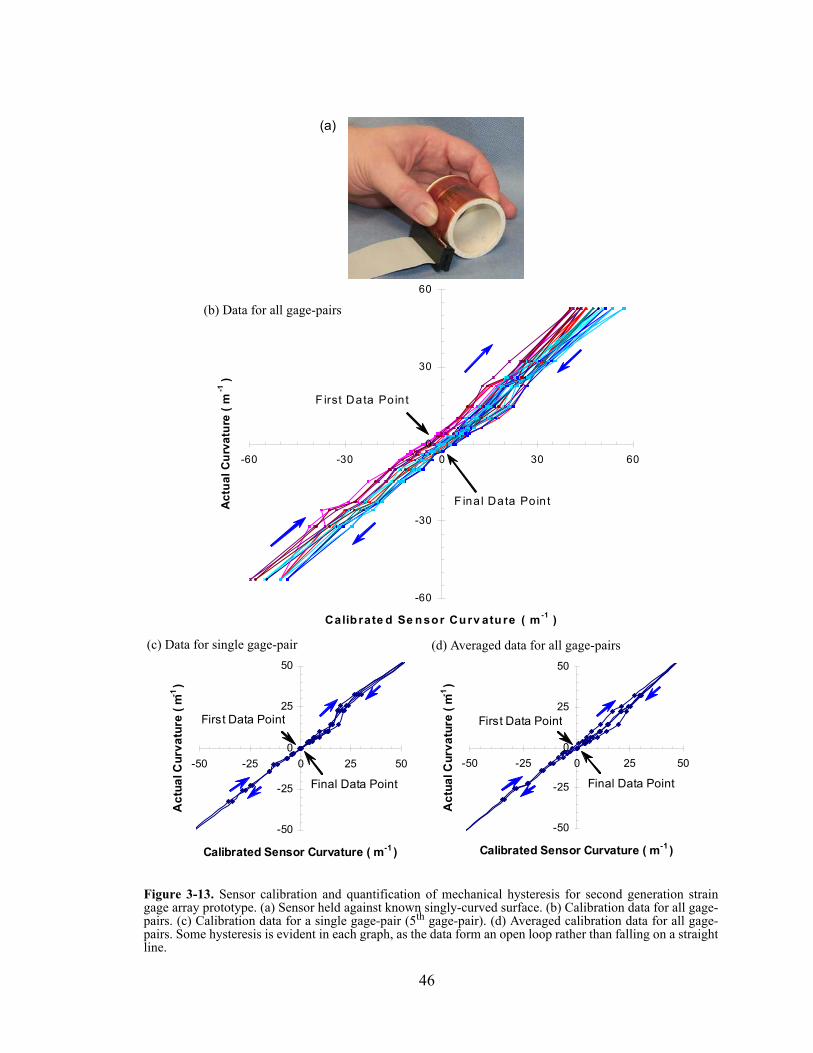
-60

-30

0

30

60

-60 -30 0 30 60

Calib rate d Se nsor Curv atu re ( m-1 )

Act

ual C

urva

ture

( m

-1 )

F irst Data Point

F inal Data Point

Figure 3-13. Sensor calibration and quantification of mechanical hysteresis for second generation strain gage array prototype. (a) Sensor held against known singly-curved surface. (b) Calibration data for all gage-pairs. (c) Calibration data for a single gage-pair (5th gage-pair). (d) Averaged calibration data for all gage-pairs. Some hysteresis is evident in each graph, as the data form an open loop rather than falling on a straight line.

(a)

-50

-25

0

25

50

-50 -25 0 25 50

Calibrated Sensor Curvature ( m-1 )

Act

ual C

urva

ture

( m-1

)

First Data Point

Final Data Point

(b) Data for all gage-pairs

-50

-25

0

25

50

-50 -25 0 25 50

Calibrated Sensor Curvature ( m-1 )

Act

ual C

urva

ture

( m-1

)

First Data Point

Final Data Point

(c) Data for single gage-pair (d) Averaged data for all gage-pairs

46

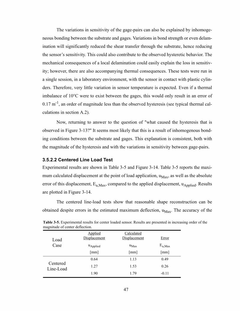
The variations in sensitivity of the gage-pairs can also be explained by inhomoge-

neous bonding between the substrate and gages. Variations in bond strength or even delam-

ination will significantly reduced the shear transfer through the substrate, hence reducing

the sensor’s sensitivity. This could also contribute to the observed hysteretic behavior. The

mechanical consequences of a local delamination could easily explain the loss in sensitiv-

ity; however, there are also accompanying thermal consequences. These tests were run in

a single session, in a laboratory environment, with the sensor in contact with plastic cylin-

ders. Therefore, very little variation in sensor temperature is expected. Even if a thermal

imbalance of 10°C were to exist between the gages, this would only result in an error of

0.17 m-1, an order of magnitude less than the observed hysteresis (see typical thermal cal-

culations in section A.2).

Now, returning to answer to the question of "what caused the hysteresis that is

observed in Figure 3-13?" It seems most likely that this is a result of inhomogenous bond-

ing conditions between the substrate and gages. This explanation is consistent, both with

the magnitude of the hysteresis and with the variations in sensitivity between gage-pairs.

3.5.2.2 Centered Line Load TestExperimental results are shown in Table 3-5 and Figure 3-14. Table 3-5 reports the maxi-

mum calculated displacement at the point of load application, uMax, as well as the absolute

error of this displacement, Eu,Max, compared to the applied displacement, uApplied. Results

are plotted in Figure 3-14.

The centered line-load tests show that reasonable shape reconstruction can be

obtained despite errors in the estimated maximum deflection, uMax. The accuracy of the

Table 3-5. Experimental results for center loaded sensor. Results are presented in increasing order of the magnitude of center deflection.

LoadCase

AppliedDisplacement

CalculatedDisplacement Error

uApplied uMax Eu,Max

[mm] [mm] [mm]

Centered Line-Load

0.64 1.13 0.49

1.27 1.53 0.26

1.90 1.79 -0.11

47

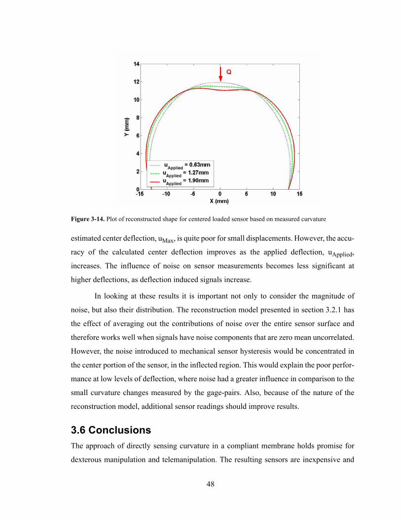
estimated center deflection, uMax, is quite poor for small displacements. However, the accu-

racy of the calculated center deflection improves as the applied deflection, uApplied,

increases. The influence of noise on sensor measurements becomes less significant at

higher deflections, as deflection induced signals increase.

In looking at these results it is important not only to consider the magnitude of

noise, but also their distribution. The reconstruction model presented in section 3.2.1 has

the effect of averaging out the contributions of noise over the entire sensor surface and

therefore works well when signals have noise components that are zero mean uncorrelated.

However, the noise introduced to mechanical sensor hysteresis would be concentrated in

the center portion of the sensor, in the inflected region. This would explain the poor perfor-

mance at low levels of deflection, where noise had a greater influence in comparison to the

small curvature changes measured by the gage-pairs. Also, because of the nature of the

reconstruction model, additional sensor readings should improve results.

3.6 ConclusionsThe approach of directly sensing curvature in a compliant membrane holds promise for

dexterous manipulation and telemanipulation. The resulting sensors are inexpensive and

Figure 3-14. Plot of reconstructed shape for centered loaded sensor based on measured curvature

48

robust and can be applied to soft, curved fingertips. Estimation of local object geometry is

computationally simple and sensor bandwidth is limited primarily by analog conversion

time. If combined with intrinsic contact sensing [Bicchi et al. 1993, and Haidacher and

Hirzinger 2002] it is possible to reduce conversion time by only sampling regions of inter-

est.

From calibration testing and thermal modeling, one can conclude that the choice

substrate is critical for good sensor performance. The substrate must have good thermal

conduction and must be uniformly bonded to the gages in order to dissipate heat and reduce

temperature gradients between the gages. Uniform bonding is also important for reducing

mechanical hysteresis. The sensor should also be isolated from the environment with a

compliant protective skin, such as silicone rubber. Not only will this protect the sensor from

damage, it also reduces heat transfer from the environment and thus reduces internal ther-

mal gradients.

Though the sensor concept is validated with this work, levels of mechanical hyster-

esis are two orders of magnitude greater than the predicted sensor resolution. Future

designs will clearly need to improve to be practical for common use.

49

4 Contact Location Display

At present, telemanipulation systems cannot approach the sensitivity and dexterity of the

human hand. To illustrate this point, imagine waking up in the dark and groping for your

glasses on the bedside table. Without much difficulty, your fingertips locate the table sur-

face and the glasses resting on it. They manipulate the glasses gently and bring them toward

your face. To attempt the same set of operations using a teleoperator would be an exercise

in frustration. Without tactile sensors at the slave and tactile displays at the master, locating

the glasses would be difficult, and attempts to manipulate the glasses would likely damage

them.

Among all the types of sensory information available in the above scenario, none is

more important than knowing where objects are touching our fingertips. Early in the study

of dexterous manipulation, Fearing [1988] demonstrated that contact information is equally

indispensable for manipulating objects in a robotic hand. Without this knowledge, grasp

errors accumulate rapidly, and the robot drops the object. Subsequently, many robotics

researchers developed tactile array sensors capable of measuring contact location, pressure

distribution, and local object geometry.

In contrast, tactile displays that render contact information for virtual reality or tele-

operation have proven far more challenging. Accurate recreation of the local shape and

pressure distribution at each fingertip requires a dense array of actuators. The peak force,

velocity, and displacement required of each element all but preclude packaging the system

at the fingertips of a standard haptic display system. The tactile displays that have appeared

in the literature are instead benchtop devices, with a small array of pins in a stationary

frame, actuated via wires or tubes [Kontarinis et al. 1995, Hasser and Weisenberger 1993,

Pawluk et al. 1998, Moy et al. 2000a].

50

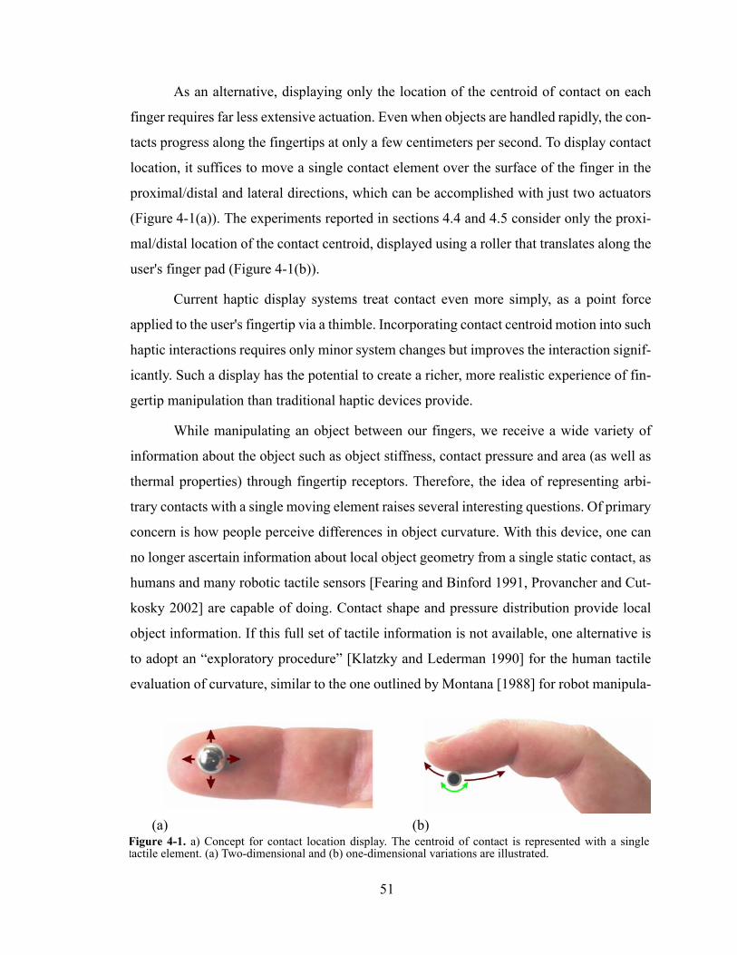
As an alternative, displaying only the location of the centroid of contact on each

finger requires far less extensive actuation. Even when objects are handled rapidly, the con-

tacts progress along the fingertips at only a few centimeters per second. To display contact

location, it suffices to move a single contact element over the surface of the finger in the

proximal/distal and lateral directions, which can be accomplished with just two actuators

(Figure 4-1(a)). The experiments reported in sections 4.4 and 4.5 consider only the proxi-

mal/distal location of the contact centroid, displayed using a roller that translates along the

user's finger pad (Figure 4-1(b)).

Current haptic display systems treat contact even more simply, as a point force

applied to the user's fingertip via a thimble. Incorporating contact centroid motion into such

haptic interactions requires only minor system changes but improves the interaction signif-

icantly. Such a display has the potential to create a richer, more realistic experience of fin-

gertip manipulation than traditional haptic devices provide.

While manipulating an object between our fingers, we receive a wide variety of

information about the object such as object stiffness, contact pressure and area (as well as

thermal properties) through fingertip receptors. Therefore, the idea of representing arbi-

trary contacts with a single moving element raises several interesting questions. Of primary

concern is how people perceive differences in object curvature. With this device, one can

no longer ascertain information about local object geometry from a single static contact, as

humans and many robotic tactile sensors [Fearing and Binford 1991, Provancher and Cut-

kosky 2002] are capable of doing. Contact shape and pressure distribution provide local

object information. If this full set of tactile information is not available, one alternative is

to adopt an “exploratory procedure” [Klatzky and Lederman 1990] for the human tactile

evaluation of curvature, similar to the one outlined by Montana [1988] for robot manipula-

Figure 4-1. a) Concept for contact location display. The centroid of contact is represented with a single tactile element. (a) Two-dimensional and (b) one-dimensional variations are illustrated.

(b)(a)

51

tors. Montana suggests that one can evaluate object curvature via rolling kinematics by

monitoring the migration of the contact patch over the finger surface during manipulation.

Contact location is also useful in other manipulation scenarios, such as pushing a knob or

slider. In these cases, the migration of the contact patch can indicate sliding or rolling of the

object relative to the finger.

To further explore these issues, I have developed a device to display contact loca-

tion together with force feedback. Two separate experiments were conducted to evaluate

the device and the user's relevant perceptions. First, subjects were asked to distinguish

between objects of different curvature for both real and virtual interactions. The second

experiment studied the perceived motion of a virtual object, simulating rolling and

anchored behaviors. The following sections outline previous work in the area of tactile dis-

play and describe the device, experiments, and conclusions.

4.1 Previous WorkMany examples of tactile displays have appeared in the literature. Typically, tactile displays

consist of an array of pin elements that move normal to the surface. These devices use a

wide range of actuator technologies: piezo-electric, shape memory alloy (SMA), electro-

magnetic, pneumatic, electrorheological, MEMS, and electrotactile. Quite often, these sys-

tems are augmented with omnidirectional vibrotactile feedback. For a review of designs

and relevant issues, see Shimoga [1993], Kaczmarek and Back-Y-Rita [1993],

Burdea [1996], Shimojo [2002] and Tachi [2002]. General design guidelines for tactile dis-

play have been reported by Fearing et al. [1997], Peine et al. [1997], Moy et al. [2000b] and

Asamura et al. [2001]. An evaluation of various actuator technologies is presented by Kam-

mermeier and Schmidt [2002].

The following subsections provide a review of previous designs, which are classi-

fied as active and passive displays. There are three general categories of active tactile dis-

plays: displays with an array of vertically-moving pins, displays with laterally-moving

elements, and electrotactile displays which stimulate cutaneous touch receptors using an

array of finely-spaced electrodes. Researchers have also investigated displays which use

materials whose mechanical properties can be modified with the application of electrical

currents, such as electrorheological (ER) materials. Since one can only discern these differ-

52

ences through active touch, the designs that utilize this actuation approach are termed "pas-

sive."

4.1.1 Vertically Moving Pin ArraysSome of the first tactile displays were adapted from braille machines. In fact some of the

early experiments were completed with such a device, the Optacon1. Most braille machines

are driven by piezoelectric actuators, which have very good bandwidth but lack the actua-

tion amplitude required to render curved surfaces with a haptic display. The performance

of piezoelectric tactile arrays can be enhanced by using bimorph (piezoelectric) actuators

as shown by Summers and Chanter [2002], but the pin displacements are still only 50 µm

or less. To address these limitations, researchers began experimenting with tactile arrays

driven by SMA (shape memory alloy) actuators [Hasser and Weisenberger 1993, Kontari-

nis et al. 1995, Taylor et al. 1995].

Two primary variations of the SMA-driven design currently exist, both which uti-

lize SMA wires to actuate their pins. In the first variation, SMA wires are placed in-line

with the axis of pin actuation and used in combination with a return spring. Such a design

is presented by Taylor et al. [1995]. They created a large area 45 x 100 pin array for display

to an entire hand.

In the second variation of SMA-driven arrays, the SMA wires run transverse to the

axis of pin actuation, allowing greater wire lengths in a thin profile package. The increased

wire length also increases total wire end-deflection. These designs incorporate various link-

ages to convert transverse SMA wire deflection to vertical pin motion.

Hasser et al. [1993, 1996] evaluated a SMA array designed by Dr. A. David Johnson

of TiNi Alloy Co. This design utilized SMA wires to pull on L-shaped beam elements in a

5 x 6 pin array. Kontarinis et al. [1995] and Wellman et al. [1998] present a design that

incorporates a linkage to transform a small amount of high-force/low-displacement actua-

tion into high-displacement pin actuation (3 mm) with a force of over 1 N. The primary

shortcomings of these designs have been device bandwidth and package size. Researchers

1. Optacon is a trademark of TeleSensory, Mountain View, CA. Optacon is no longer in business, though an Israeli company, Virtouch Ltd, now sells an inexpensive mouse which includes two braille cells (the VirTouch Mouse, VTM, for about $700).

53

have optimized bandwidth with clever control schemes and by water-cooling the SMA

wires [Howe et al. 1995]. Displays with a single line of pins have also been built to reduce

package size. These devices can be placed on robotic masters for telepalpation [Peine et

al. 1994].

In an effort to further improve device bandwidth, researchers have investigated

designs driven by solenoids [Fischer et al. 1995], voice-coils [Pawluk et al. 1998], and

other electromagnetic actuators. Kammermeier et al. [2000] produced a 6 x 6 pin array

(3mm pin spacing) driven by electro-magnetic rocker-lever actuators driven open-loop.

With this design, they are able to accomplish an actuation stroke of 1.6 mm at 4.5 N and an

impressive bandwidth exceeding 100 Hz. Fukuda et al. [1997] used an array (3 x 3) of elec-

tromagnetic resonators in their device.

Researchers have also pursued pneumatic designs driven by the desire to make

these devices more compact and lightweight [Cohn et al. 1992, Caldwell et al. 1999, Moy

et al. 2000a]. Cohn et al. [1992] present one of the first pnuematically-actuated tactile dis-

plays composed of an array of pneumatic cylinders. Moy et al. [2000a] have designed a

5 Hz display composed of a 5 x 5 array of small air pockets driven via PWM with binary

valves. Binary valves were chosen because of their suitability for miniaturization. The dis-

play is fastened to a user’s fingertip, supplied with air, and controlled by an external source

via individual air lines. Caldwell et al. [1999] report a similar glove-based design that also

supplies vibrotactile and either thermal or shear feedback. Caldwell et al. accomplish an

impressive 11 Hz on the 4 x 4 array with proportionally-controlled valves. Asamura et al.

[1998] have similarly augmented their device by adding vibrotactile feedback to an array

of airjets. In fact, many researchers have augmented their devices with vibrotactile feed-

back. Kontarinis and Howe [1995] show that vibrotactile feedback can be a simple yet

effective way to display the high frequency content present during slip and collision. They

show that even a single voice-coil actuator improves performance. Furthermore, the orien-

tation of the vibrating element does not appear to be critical, thus allowing flexible pack-

aging.

Several researchers have taken a more pragmatic approach to the design of tactile

displays by using commercially available servomotors in their design [Wagner et al. 2002,

54

Iwata et al. 2001]. Wagner et al. [2002] present a tiered 6 x 6 construction with a small

motion bandwidth of 25 Hz accomplished with commercial RC servo motors. Iwata et al.

[2001] present a full hand tactile display with pins driven by DC motors and leadscrews.

In the interests of further miniaturization, Ghodssi et al. [1996] present one of the

first MEMS-based tactile arrays. Siegel [2002] reports another interesting MEMS array

designed by Fedder and Lopez2 at Carnegie-Mellon. Fedder and Lopez use electrostatic

forces to actuate their MEMS array. Each element of their array contains air trapped

between a metal-coated polymer membrane and silicon substrate. Each element consists of

a center chamber connected to an annular chamber. When an attractive electrostatic charge

is applied to the annular region, that portion of the membrane collapses, forcing the air to

bulge the central tactile element. With the ongoing goal of producing tactile displays at a

smaller scale, one may expect to see more MEMS designs emerge in the future.

4.1.2 Laterally Moving Pin ArraysAnother novel display design is presented by Hayward et al. [2000]. Their design utilizes

an array of 64 piezoelectric actuators that move an array of 112 pins laterally rather than

normal to the surface of the skin. This device presents distributed skin stretch3. It is partic-

ularly attractive because of its small relative size and ability to integrate with device elec-

tronics.

4.1.3 Electrotactile ArraysUltimately, one might like to provide sensation directly to the nerve endings of the finger,

thus eliminating the need for external hardware. As a middle ground, researchers such as

Tang and Beebe [1998] provide electrostatic4 feedback to the fingerpad of a user in a band-

aid sized package. However, despite the advantages of slim packaging, users have not

embraced it due to discomfort. For a more in depth review of this technology (as well as

vibrotactile feedback), see Kaczmarek et al. [1991].

2. http://www.ri.cmu.edu/projects/project_470.html3. Immersion corp. developed a trackpad for laptop computers which incorporated lateral motion of the entire trackpad, for tactile feedback. However, the trackpad was never commercialized.4. Electrostatic is a voltage-controlled form of electrotactile feedback (which is current based)

55

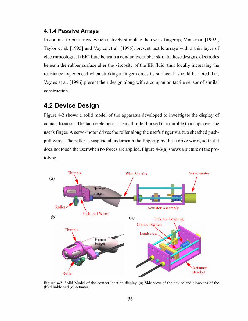
4.1.4 Passive ArraysIn contrast to pin arrays, which actively stimulate the user’s fingertip, Monkman [1992],

Taylor et al. [1995] and Voyles et al. [1996], present tactile arrays with a thin layer of

electrorheological (ER) fluid beneath a conductive rubber skin. In these designs, electrodes

beneath the rubber surface alter the viscosity of the ER fluid, thus locally increasing the

resistance experienced when stroking a finger across its surface. It should be noted that,

Voyles et al. [1996] present their design along with a companion tactile sensor of similar

construction.

4.2 Device DesignFigure 4-2 shows a solid model of the apparatus developed to investigate the display of

contact location. The tactile element is a small roller housed in a thimble that slips over the

user's finger. A servo-motor drives the roller along the user's finger via two sheathed push-

pull wires. The roller is suspended underneath the fingertip by these drive wires, so that it

does not touch the user when no forces are applied. Figure 4-3(a) shows a picture of the pro-

totype.

Figure 4-2. Solid Model of the contact location display. (a) Side view of the device and close-ups of the (b) thimble and (c) actuator.

(a)

(b) (c)

Wire SheathsThimble Servo-motor

Actuator AssemblyRollerPush-pull Wires

HumanFinger

HumanFinger

Thimble

Roller

Flexible Coupling

Leadscrew

Contact Switch

ActuatorBracket

56

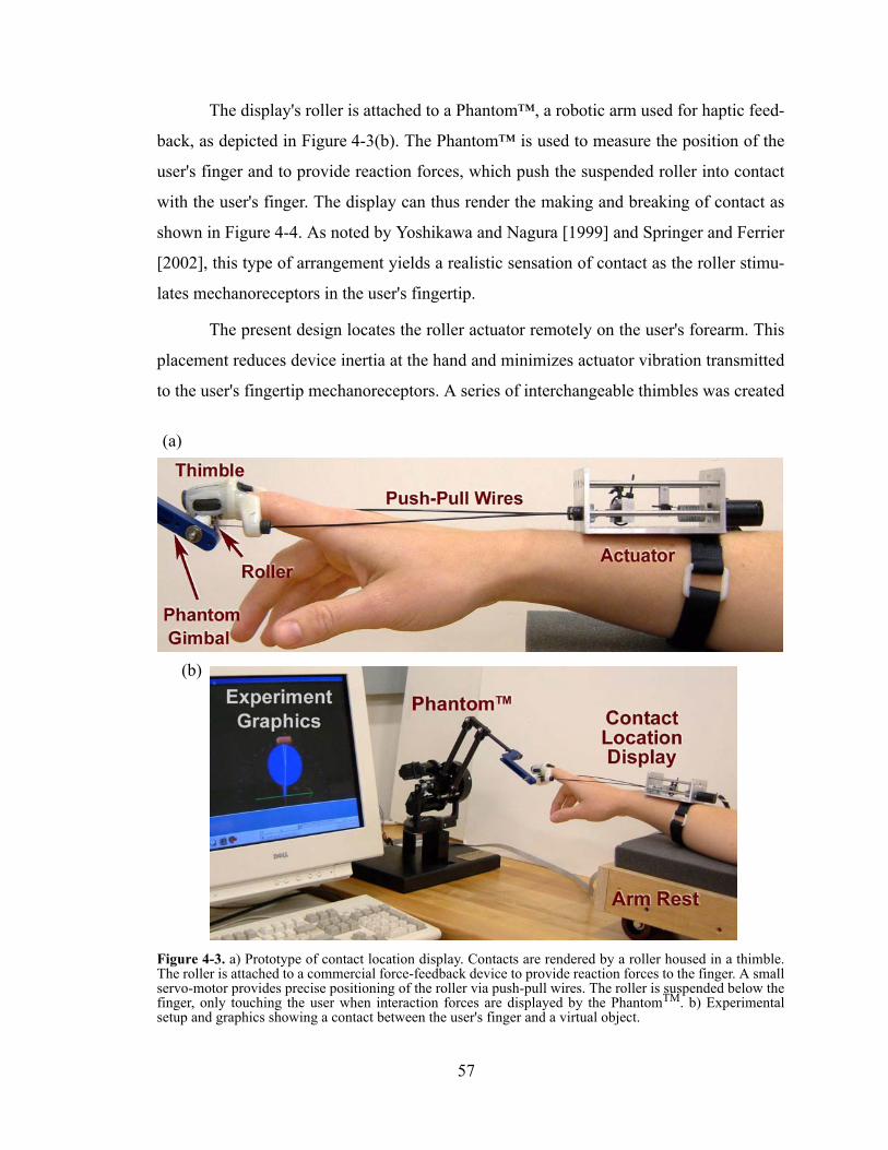
The display's roller is attached to a Phantom™, a robotic arm used for haptic feed-

back, as depicted in Figure 4-3(b). The Phantom™ is used to measure the position of the

user's finger and to provide reaction forces, which push the suspended roller into contact

with the user's finger. The display can thus render the making and breaking of contact as

shown in Figure 4-4. As noted by Yoshikawa and Nagura [1999] and Springer and Ferrier

[2002], this type of arrangement yields a realistic sensation of contact as the roller stimu-

lates mechanoreceptors in the user's fingertip.

The present design locates the roller actuator remotely on the user's forearm. This

placement reduces device inertia at the hand and minimizes actuator vibration transmitted

to the user's fingertip mechanoreceptors. A series of interchangeable thimbles was created

Figure 4-3. a) Prototype of contact location display. Contacts are rendered by a roller housed in a thimble. The roller is attached to a commercial force-feedback device to provide reaction forces to the finger. A small servo-motor provides precise positioning of the roller via push-pull wires. The roller is suspended below the finger, only touching the user when interaction forces are displayed by the PhantomTM. b) Experimental setup and graphics showing a contact between the user's finger and a virtual object.

(a)

(b)

57

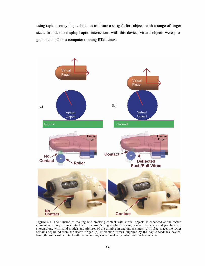
using rapid-prototyping techniques to insure a snug fit for subjects with a range of finger

sizes. In order to display haptic interactions with this device, virtual objects were pro-

grammed in C on a computer running RTai Linux.

Figure 4-4. The illusion of making and breaking contact with virtual objects is enhanced as the tactile element is brought into contact with the user’s finger when making contact. Experimental graphics are shown along with solid models and pictures of the thimble in analogous states. (a) In free-space, the roller remains separated from the user’s finger. (b) Interaction forces, supplied by the haptic feedback device, bring the roller into contact with the users finger when making contact with virtual objects.

(a) (b)

HumanFinger

HumanFinger

58

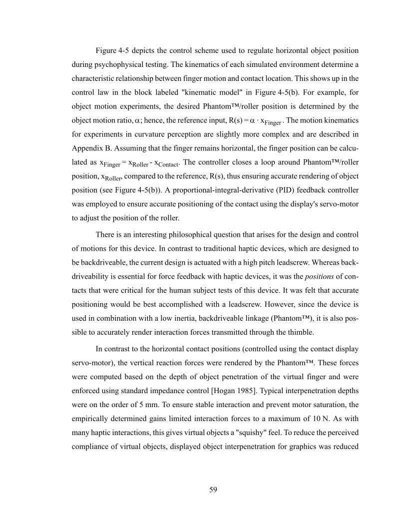
Figure 4-5 depicts the control scheme used to regulate horizontal object position

during psychophysical testing. The kinematics of each simulated environment determine a

characteristic relationship between finger motion and contact location. This shows up in the

control law in the block labeled "kinematic model" in Figure 4-5(b). For example, for

object motion experiments, the desired Phantom™/roller position is determined by the

object motion ratio, α; hence, the reference input, R(s) = α · xFinger . The motion kinematics

for experiments in curvature perception are slightly more complex and are described in

Appendix B. Assuming that the finger remains horizontal, the finger position can be calcu-

lated as xFinger = xRoller - xContact. The controller closes a loop around Phantom™/roller

position, xRoller, compared to the reference, R(s), thus ensuring accurate rendering of object

position (see Figure 4-5(b)). A proportional-integral-derivative (PID) feedback controller

was employed to ensure accurate positioning of the contact using the display's servo-motor

to adjust the position of the roller.

There is an interesting philosophical question that arises for the design and control

of motions for this device. In contrast to traditional haptic devices, which are designed to

be backdriveable, the current design is actuated with a high pitch leadscrew. Whereas back-

driveability is essential for force feedback with haptic devices, it was the positions of con-

tacts that were critical for the human subject tests of this device. It was felt that accurate

positioning would be best accomplished with a leadscrew. However, since the device is

used in combination with a low inertia, backdriveable linkage (Phantom™), it is also pos-

sible to accurately render interaction forces transmitted through the thimble.

In contrast to the horizontal contact positions (controlled using the contact display

servo-motor), the vertical reaction forces were rendered by the Phantom™. These forces

were computed based on the depth of object penetration of the virtual finger and were

enforced using standard impedance control [Hogan 1985]. Typical interpenetration depths

were on the order of 5 mm. To ensure stable interaction and prevent motor saturation, the

empirically determined gains limited interaction forces to a maximum of 10 N. As with

many haptic interactions, this gives virtual objects a "squishy" feel. To reduce the perceived

compliance of virtual objects, displayed object interpenetration for graphics was reduced

59

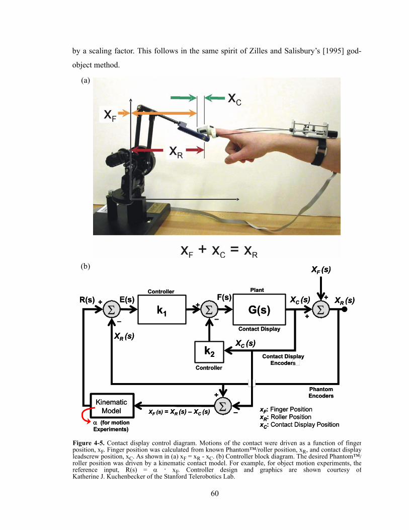
by a scaling factor. This follows in the same spirit of Zilles and Salisbury’s [1995] god-

object method.

Σ k1 G(s) ΣE(s)R(s)

XF (s)

XR (s)XC (s)+ +

+–

XR (s)

Σ

k2

F(s)

–

+

XC (s)

Σ+

–XF (s) = XR (s) – XC (s) xF: Finger PositionxR: Roller PositionxC: Contact Display Position

PhantomEncoders

Contact DisplayEncoders

Contact Display

KinematicModel

Controller

Controller

Plant

α (for motionExperiments)

Σ k1 G(s) ΣE(s)R(s)

XF (s)

XR (s)XC (s)+ +

+–

XR (s)

Σ

k2

F(s)

–

+

XC (s)

Σ+

–XF (s) = XR (s) – XC (s) xF: Finger PositionxR: Roller PositionxC: Contact Display Position

PhantomEncoders

Contact DisplayEncoders

Contact Display

KinematicModel

Controller

Controller

Plant

α (for motionExperiments)

Figure 4-5. Contact display control diagram. Motions of the contact were driven as a function of fingerposition, xF. Finger position was calculated from known Phantom™/roller position, xR, and contact displayleadscrew position, xC. As shown in (a) xF = xR - xC. (b) Controller block diagram. The desired Phantom™/roller position was driven by a kinematic contact model. For example, for object motion experiments, thereference input, R(s) = α · xF. Controller design and graphics are shown courtesy ofKatherine J. Kuchenbecker of the Stanford Telerobotics Lab.

(a)

(b)

60

The small motion closed-loop bandwidth of the roller exceeds 5 Hz for a travel of

10 mm (the actual bandwidth was determined by driving the roller with a 10 mm pk-pk

sinusoidal input was determined to be approximately 8 Hz). Roller positions along the

finger are rendered with a maximum error of 0.05 mm for fast hand motions (5 cm/sec) and

an error of about 0.01 mm for the slow motions typically used by subjects. For additional

details of the device design see Appendix B.

4.3 Experimental Goals and ApproachTwo sets of experiments were conducted to evaluate the device and the merits of displaying

contact location to users. Of primary concern is how subjects interpret virtual object inter-

actions when each of the contacts is represented by the same (constant curvature) tactile

element (a roller). To investigate this effect, a first set of experiments was constructed in

which object kinematics were directly proportional to object curvature. Subjects were

asked to distinguish between objects of different curvature for both real and virtual interac-

tions. The experiments in perception of object curvature are described in section 4.4. In a

second set of experiments, described in section 4.5, subjects discriminated between objects

with differing motion conditions. The motion of the virtual objects rendered in these exper-

iments was independent of object radius.

The goal of the two sets of experiments is to answer the following questions:

• How does a subject’s ability to discriminate between objects of varying curvature

handled directly compare to his ability when handling virtual objects rendered via the

contact location display?

• Can subjects identify motion conditions, found in prototypical manipulation tasks, of

virtual objects rendered via contact location display?

The following subsection describes the framework and detailed protocol followed in both

experiments.

4.3.1 General Experimental ProtocolBoth of the conducted experiments followed the same general protocol. The experimental

approach was reviewed by established researchers in the fields of psychophysics and neu-

61

rphysiology5 and followed closely to the methods outlined by Gescheider [1997]. For a

general review of classical psychophysical methods, refer back to chapter 2 of this thesis.

All experiments employed the method of constant stimuli with a paired-comparison

forced-choice protocol to evaluate perceptual thresholds (JNDs) and sensitivity. To inves-

tigate perceptual sensitivity over a broad range, the experiment was divided into blocks. In

each block, subjects were presented with stimuli clustered around a nominal value, referred

to as a standard stimulus. Each standard was accompanied by six comparison stimuli (three

larger and three smaller, presented twice each). Subjects were presented with two stimuli

in rapid succession (separated by 2-4 seconds) and asked to state which met the specified

condition. Standard precautions were taken to prevent presentation order bias. To isolate

the effects of learning and fatigue, half of the subjects completed virtual discrimination

experiments first. Subjects were blindfolded and wore hunter's earmuffs to reduce distrac-

tions and ambient noise.

Sighted and blindfolded training preceded each block of testing. Virtual simulations

were accompanied by computer graphics to reinforce haptic cues during training. Positive

feedback on discrimination accuracy was provided at the beginning of curvature discrimi-

nation experiments. However, it was not provided in motion discrimination experiments to

prevent habituation.

All subjects completed the experiment using the index finger of their right hand. For

consistency between virtual- and direct-discrimination experiments, subjects performed

these tests with their fingers extended and horizontal. The virtual apparatus did not measure

rotations of the subject's finger, and kinematic modeling assumed that the finger orientation

was always horizontal. The subject's fingers were placed at the center of each stimulus.

They made a single sustained contact with each stimulus and were not to allowed to slide

on the stimulus' surface while exploring the physical models.

There were no time restrictions made on subjects during testing. However, to min-

imize the time required of each subject, tests were completed by two test groups. A majority

of subjects completed the test in under one-and-a-half hours. There were 14 people in the

5. Experiments were discussed in pilot testing stage with Susan Lederman of Queens University and Man-dayam Srinivasan of MIT.

62

first test group, which consisted of 10 males and 4 females ranging in age from 20 to 34.

All subjects in this group were right-handed. There were 10 people in the second group,

which consisted of 8 males and 2 females ranging in age from 20 to 38. Two of the males

in the second group were left handed. The number of people completing virtual or direct

experiments first was equally balanced (i.e., for the second group, 1 left-handed male and

3 right-handed males, and 1 right-handed female completed the virtual experiments first).

Subjects completed a short questionnaire at the conclusion of the experiments.

4.4 Curvature Discrimination for Real and Virtual ObjectsA series of experiments was performed to quantify a user's ability to discriminate between

objects of varying curvature. To simplify testing, only planar objects were studied and the

interaction was limited to horizontal motion of a single finger. This simplification allowed

a direct comparison of results between direct physical manipulation and manipulation with

virtual objects via the contact display device.

As outlined in section 4.3.1, the experiments were designed following standard psy-

chophysical procedures involving constant stimuli, with forced-choice comparisons

between pairs of cases [Gescheider 1997].

4.4.1 Experimental ProcedureThese discrimination tests focused on the user's perception of curvature while rolling planar

objects with a single finger. As illustrated in Figure 4-6(a), such simple one-fingered inter-

action is representative of more general object manipulation. All objects, whether real or

virtual, pivoted about a fixed axis distinct from the centers of curvature. This pivoting

motion allowed the user to explore the curved surface using only a fingertip movement. For

convenience, fourteen test curves were arranged onto a single "curvature wheel,'' as is

shown in Figure 4-6(b). Two wheels were used for the experiments, each with stimuli for

two standards. For each curve, the wheel could pivot 15°, corresponding to approximately

±1 cm of fingertip movement. The radius of curvature of the objects varied from 8.3 mm

to 52.6 mm.

During the tests, subjects were blindfolded and used an armrest to maintain a hori-

zontal hand position. Both real and virtual versions of the curvature wheel were presented

63

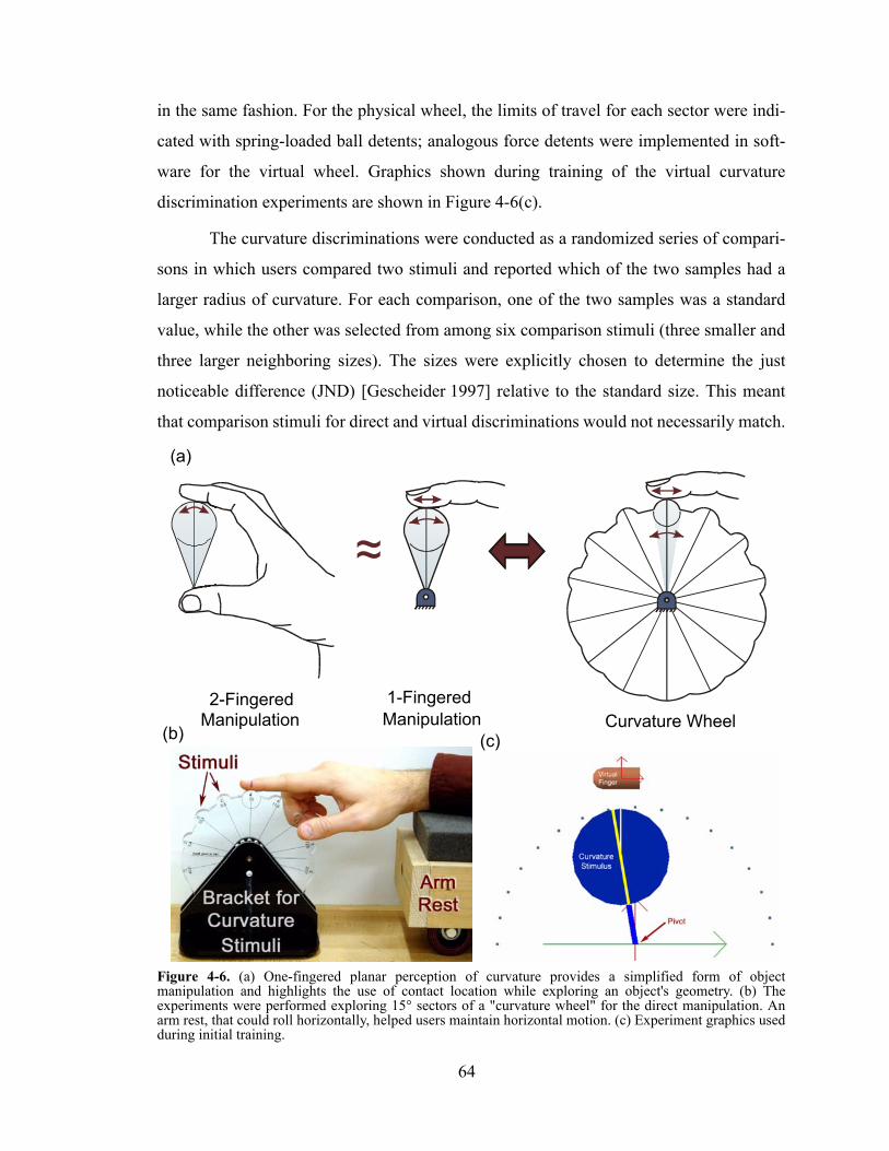
in the same fashion. For the physical wheel, the limits of travel for each sector were indi-

cated with spring-loaded ball detents; analogous force detents were implemented in soft-

ware for the virtual wheel. Graphics shown during training of the virtual curvature

discrimination experiments are shown in Figure 4-6(c).

The curvature discriminations were conducted as a randomized series of compari-

sons in which users compared two stimuli and reported which of the two samples had a

larger radius of curvature. For each comparison, one of the two samples was a standard

value, while the other was selected from among six comparison stimuli (three smaller and

three larger neighboring sizes). The sizes were explicitly chosen to determine the just

noticeable difference (JND) [Gescheider 1997] relative to the standard size. This meant

that comparison stimuli for direct and virtual discriminations would not necessarily match.

Figure 4-6. (a) One-fingered planar perception of curvature provides a simplified form of object manipulation and highlights the use of contact location while exploring an object's geometry. (b) The experiments were performed exploring 15° sectors of a "curvature wheel" for the direct manipulation. An arm rest, that could roll horizontally, helped users maintain horizontal motion. (c) Experiment graphics used during initial training.

~~

(a)

(b)

2-FingeredManipulation Manipulation

1-FingeredCurvature Wheel

(c)

64

Gescheider [1997] recommends selecting comparison stimuli such that the easiest to dis-

tinguish from the standard (the largest and smallest stimuli) can be identified approximately

90% of the time. The remaining comparison stimuli are equally spaced between the

extremes and the standard. As with any psychophysical experiment, pilot tests were con-

ducted to ensure that stimuli were appropriately chosen. Pilot testing is essential to the suc-

cess of any set of perceptual experiments, as one can improve procedure or modify the tests

performed before making a more significant time investment during subject tests. Subjects

made curvature discriminations with respect to four radius standards ranging from 10 mm

to 40 mm.

4.4.2 Results and Discussion of Curvature Discrimination Experiments

Results for direct and virtual curvature comparison tests are shown in Table 4-1 and

Figure 4-7. The graphs in Figure 4-7 represent the pooled responses of all subjects for 10,

20, 30, and 40 mm standards. They plot the proportion of times subjects reported each stim-

ulus as the larger of the two presented.

65

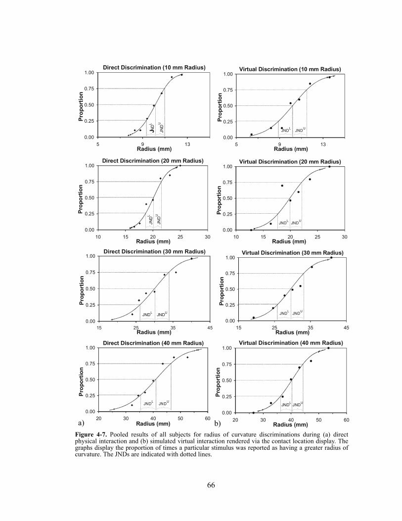
Virtual Discrimination (40 mm Radius)

0.00

0.25

0.50

0.75

1.00

20 30 40 50 60Radius (mm)

Prop

ortio

n

JNDL JNDU

Virtual Discrimination (30 mm Radius)

0.00

0.25

0.50

0.75

1.00

15 25 35 45Radius (mm)

Prop

ortio

n

JNDL JNDU

Direct Discrimination (20 mm Radius)

0.00

0.25

0.50

0.75

1.00

10 15 20 25 30Radius (mm)

Prop

ortio

n

JND

L

JND

U

Virtual Discrimination (20 mm Radius)

0.00

0.25

0.50

0.75

1.00

10 15 20 25 30Radius (mm)

Prop

ortio

nJNDL JNDU

0.00

0.25

0.50

0.75

1.00

15 25 35 45Radius (mm)

Prop

ortio

n

JNDL JNDU

Direct Discrimination (30 mm Radius)

Direct Discrimination (10 mm Radius)

0.00

0.25

0.50

0.75

1.00

5 9 13Radius (mm)

Prop

ortio

n

JND

L

JND

U

Virtual Discrimination (10 mm Radius)

0.00

0.25

0.50

0.75

1.00

5 9 13Radius (mm)

Prop

ortio

n

JNDL JNDU

Direct Discrimination (40 mm Radius)

0.00

0.25

0.50

0.75

1.00

20 30 40 50 60Radius (mm)

Prop

ortio

n

JNDL JNDU

a) b)Figure 4-7. Pooled results of all subjects for radius of curvature discriminations during (a) direct physical interaction and (b) simulated virtual interaction rendered via the contact location display. The graphs display the proportion of times a particular stimulus was reported as having a greater radius of curvature. The JNDs are indicated with dotted lines.

66

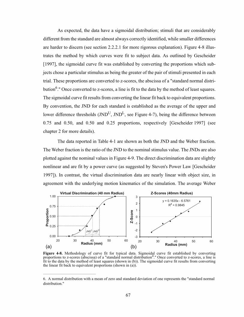
As expected, the data have a sigmoidal distribution; stimuli that are considerably

different from the standard are almost always correctly identified, while smaller differences

are harder to discern (see section 2.2.2.1 for more rigorous explanation). Figure 4-8 illus-

trates the method by which curves were fit to subject data. As outlined by Gescheider

[1997], the sigmoidal curve fit was established by converting the proportions which sub-

jects chose a particular stimulus as being the greater of the pair of stimuli presented in each

trial. These proportions are converted to z-scores, the abscissa of a "standard normal distri-

bution6." Once converted to z-scores, a line is fit to the data by the method of least squares.

The sigmoidal curve fit results from converting the linear fit back to equivalent proportions.

By convention, the JND for each standard is established as the average of the upper and

lower difference thresholds (JNDU, JNDL, see Figure 4-7), being the difference between

0.75 and 0.50, and 0.50 and 0.25 proportions, respectively [Gescheider 1997] (see

chapter 2 for more details).

The data reported in Table 4-1 are shown as both the JND and the Weber fraction.

The Weber fraction is the ratio of the JND to the nominal stimulus value. The JNDs are also

plotted against the nominal values in Figure 4-9. The direct discrimination data are slightly

nonlinear and are fit by a power curve (as suggested by Steven's Power Law [Gescheider

1997]). In contrast, the virtual discrimination data are nearly linear with object size, in

agreement with the underlying motion kinematics of the simulation. The average Weber

6. A normal distribution with a mean of zero and standard deviation of one represents the "standard normal distribution."

Figure 4-8. Methodology of curve fit for typical data. Sigmoidal curve fit established by converting proportions to z-scores (abscissa) of a "standard normal distribution4." Once converted to z-scores, a line is fit to the data by the method of least squares (shown in (b)). The sigmoidal curve fit results from converting the linear fit back to equivalent proportions (shown in (a)).

Virtual Discrimination (40 mm Radius)

0.00

0.25

0.50

0.75

1.00

20 30 40 50 60Radius (mm)

Prop

ortio

n

JNDL JNDU

Z-Scores (40mm Radius)

y = 0.1635x - 6.5761R2 = 0.9845

-3

-2

-1

0

1

2

3

20 30 40 50 60Radius (mm)

Z-Sc

ore

(a) (b)

67

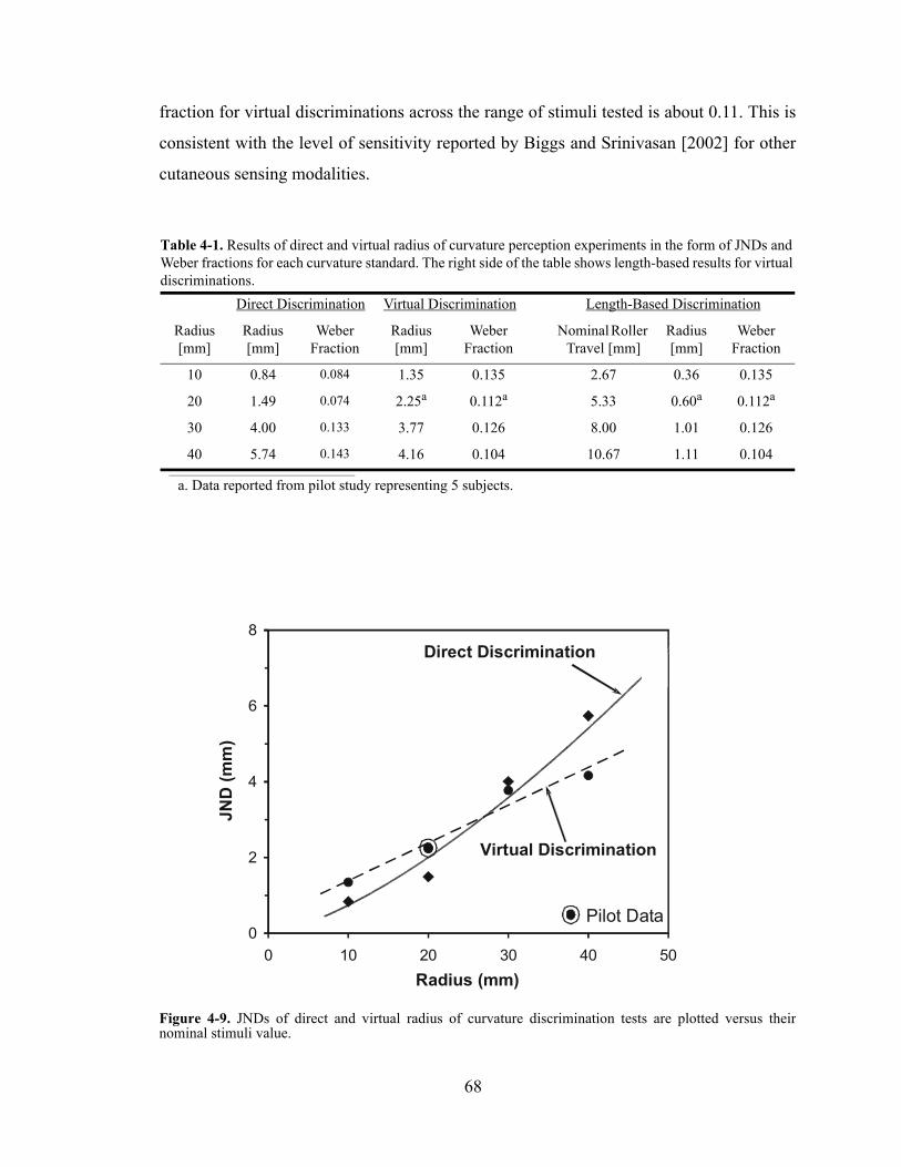
fraction for virtual discriminations across the range of stimuli tested is about 0.11. This is

consistent with the level of sensitivity reported by Biggs and Srinivasan [2002] for other

cutaneous sensing modalities.

Table 4-1. Results of direct and virtual radius of curvature perception experiments in the form of JNDs and Weber fractions for each curvature standard. The right side of the table shows length-based results for virtual discriminations.

Radius[mm]

Direct Discrimination Virtual Discrimination Length-Based Discrimination

Radius[mm]

Weber Fraction

Radius[mm]

Weber Fraction

Nominal Roller Travel [mm]

Radius[mm]

Weber Fraction

10 0.84 0.084 1.35 0.135 2.67 0.36 0.135

20 1.49 0.074 2.25a

a. Data reported from pilot study representing 5 subjects.

0.112a 5.33 0.60a 0.112a

30 4.00 0.133 3.77 0.126 8.00 1.01 0.126

40 5.74 0.143 4.16 0.104 10.67 1.11 0.104

Figure 4-9. JNDs of direct and virtual radius of curvature discrimination tests are plotted versus their nominal stimuli value.

0

2

4

6

8

0 10 20 30 40 50Radius (mm)

JND

(mm

)

Direct Discrimination

Virtual Discrimination

Pilot Data

68

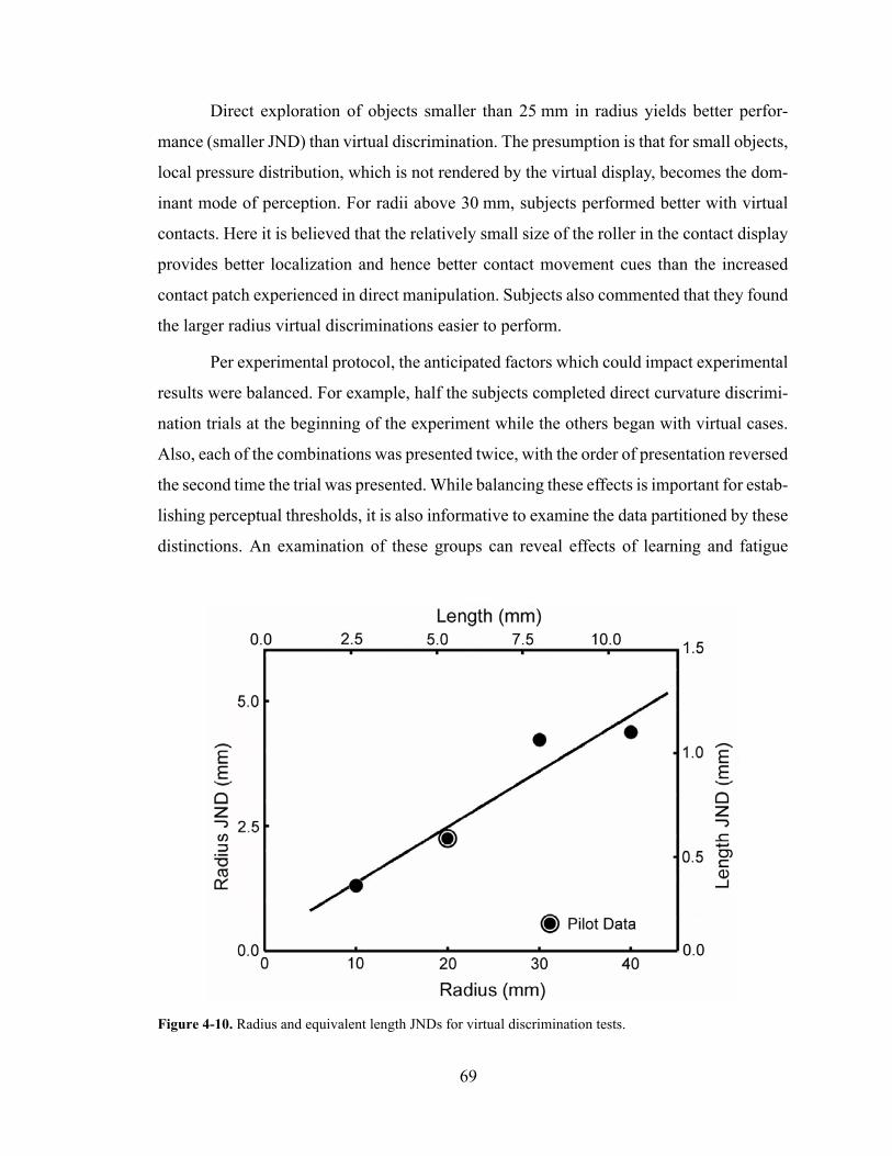
Direct exploration of objects smaller than 25 mm in radius yields better perfor-

mance (smaller JND) than virtual discrimination. The presumption is that for small objects,

local pressure distribution, which is not rendered by the virtual display, becomes the dom-

inant mode of perception. For radii above 30 mm, subjects performed better with virtual

contacts. Here it is believed that the relatively small size of the roller in the contact display

provides better localization and hence better contact movement cues than the increased

contact patch experienced in direct manipulation. Subjects also commented that they found

the larger radius virtual discriminations easier to perform.

Per experimental protocol, the anticipated factors which could impact experimental

results were balanced. For example, half the subjects completed direct curvature discrimi-

nation trials at the beginning of the experiment while the others began with virtual cases.

Also, each of the combinations was presented twice, with the order of presentation reversed

the second time the trial was presented. While balancing these effects is important for estab-

lishing perceptual thresholds, it is also informative to examine the data partitioned by these

distinctions. An examination of these groups can reveal effects of learning and fatigue

Figure 4-10. Radius and equivalent length JNDs for virtual discrimination tests.

69

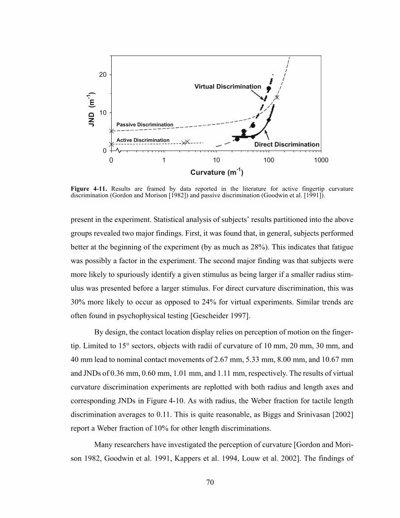
present in the experiment. Statistical analysis of subjects’ results partitioned into the above

groups revealed two major findings. First, it was found that, in general, subjects performed

better at the beginning of the experiment (by as much as 28%). This indicates that fatigue

was possibly a factor in the experiment. The second major finding was that subjects were

more likely to spuriously identify a given stimulus as being larger if a smaller radius stim-

ulus was presented before a larger stimulus. For direct curvature discrimination, this was

30% more likely to occur as opposed to 24% for virtual experiments. Similar trends are

often found in psychophysical testing [Gescheider 1997].

By design, the contact location display relies on perception of motion on the finger-

tip. Limited to 15° sectors, objects with radii of curvature of 10 mm, 20 mm, 30 mm, and

40 mm lead to nominal contact movements of 2.67 mm, 5.33 mm, 8.00 mm, and 10.67 mm

and JNDs of 0.36 mm, 0.60 mm, 1.01 mm, and 1.11 mm, respectively. The results of virtual

curvature discrimination experiments are replotted with both radius and length axes and

corresponding JNDs in Figure 4-10. As with radius, the Weber fraction for tactile length

discrimination averages to 0.11. This is quite reasonable, as Biggs and Srinivasan [2002]

report a Weber fraction of 10% for other length discriminations.

Many researchers have investigated the perception of curvature [Gordon and Mori-

son 1982, Goodwin et al. 1991, Kappers et al. 1994, Louw et al. 2002]. The findings of

Figure 4-11. Results are framed by data reported in the literature for active fingertip curvature discrimination (Gordon and Morison [1982]) and passive discrimination (Goodwin et al. [1991]).

0

10

20

0.1 1 10 100 1000

Curvature (m-1)

JND

(m-1

)

Direct Discrimination

Virtual Discrimination

Passive Discrimination

Active Discrimination

0

70

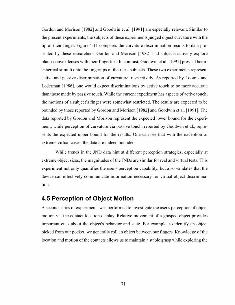
Gordon and Morison [1982] and Goodwin et al. [1991] are especially relevant. Similar to

the present experiments, the subjects of these experiments judged object curvature with the

tip of their finger. Figure 4-11 compares the curvature discrimination results to data pre-

sented by these researchers. Gordon and Morison [1982] had subjects actively explore

plano-convex lenses with their fingertips. In contrast, Goodwin et al. [1991] pressed hemi-

spherical stimuli onto the fingertips of their test subjects. These two experiments represent

active and passive discrimination of curvature, respectively. As reported by Loomis and

Lederman [1986], one would expect discriminations by active touch to be more accurate

than those made by passive touch. While the current experiment has aspects of active touch,

the motions of a subject’s finger were somewhat restricted. The results are expected to be

bounded by those reported by Gordon and Morison [1982] and Goodwin et al. [1991]. The

data reported by Gordon and Morison represent the expected lower bound for the experi-

ment, while perception of curvature via passive touch, reported by Goodwin et al., repre-

sents the expected upper bound for the results. One can see that with the exception of

extreme virtual cases, the data are indeed bounded.

While trends in the JND data hint at different perception strategies, especially at

extreme object sizes, the magnitudes of the JNDs are similar for real and virtual tests. This

experiment not only quantifies the user's perception capability, but also validates that the

device can effectively communicate information necessary for virtual object discrimina-

tion.

4.5 Perception of Object MotionA second series of experiments was performed to investigate the user's perception of object

motion via the contact location display. Relative movement of a grasped object provides

important cues about the object's behavior and state. For example, to identify an object

picked from our pocket, we generally roll an object between our fingers. Knowledge of the

location and motion of the contacts allows us to maintain a stable grasp while exploring the

71

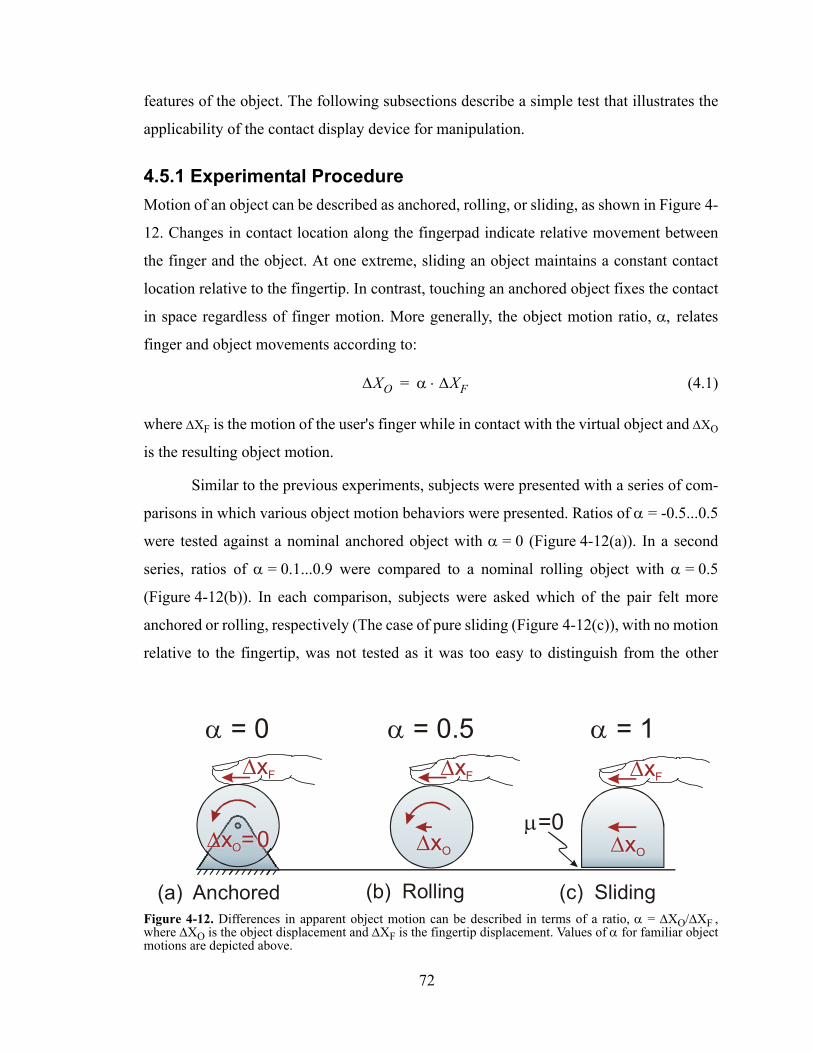
features of the object. The following subsections describe a simple test that illustrates the

applicability of the contact display device for manipulation.

4.5.1 Experimental ProcedureMotion of an object can be described as anchored, rolling, or sliding, as shown in Figure 4-

12. Changes in contact location along the fingerpad indicate relative movement between

the finger and the object. At one extreme, sliding an object maintains a constant contact

location relative to the fingertip. In contrast, touching an anchored object fixes the contact

in space regardless of finger motion. More generally, the object motion ratio, α, relates

finger and object movements according to:

(4.1)

where ∆XF is the motion of the user's finger while in contact with the virtual object and ∆XO

is the resulting object motion.

Similar to the previous experiments, subjects were presented with a series of com-

parisons in which various object motion behaviors were presented. Ratios of α = -0.5...0.5

were tested against a nominal anchored object with α = 0 (Figure 4-12(a)). In a second

series, ratios of α = 0.1...0.9 were compared to a nominal rolling object with α = 0.5

(Figure 4-12(b)). In each comparison, subjects were asked which of the pair felt more

anchored or rolling, respectively (The case of pure sliding (Figure 4-12(c)), with no motion

relative to the fingertip, was not tested as it was too easy to distinguish from the other

Figure 4-12. Differences in apparent object motion can be described in terms of a ratio, α = ∆XO/∆XF , where ∆XO is the object displacement and ∆XF is the fingertip displacement. Values of α for familiar object motions are depicted above.

α = 0 α = 0.5 α = 1

µ=0

∆xF

∆xO

∆xF

∆x =0O

∆xF

∆xO

(a) Anchored (b) Rolling (c) Sliding

∆XO α ∆XF⋅=

72

cases). The graphics that accompanied initial training for each subject are shown in

Figure 4-13.

4.5.2 Results and Discussion of Object Motion ExperimentsFigures 4-14(a) and 4-14(b) show the proportions of times that subjects identified a virtual

object with a given value of α as anchored or freely rolling, respectively.

It is believed that people evaluated object motion based on a comparison between

absolute finger movement, observed via proprioception, and relative contact centroid

movement, observed cutaneously. Based on the results of curvature discrimination experi-

ment, the cutaneous contribution to this comparison is quite accurate. Proprioceptive length

estimates are not nearly as good, which could explain the spread of the data. The standard

deviation for rolling object tests was substantially smaller than for anchored objects, which

can be attributed to peoples' experience rolling and manipulating objects in their hands.

The means of the anchored and rolling distributions are -0.09 and 0.56, respectively,

falling close to their nominal values of 0.0 and 0.5. This mismatch is an interesting percep-

tual result of these unsighted object manipulations, though its exact origin is unknown. Par-

ticularly noteworthy is users' preference for negative ratios in the anchored object tests.

Unlike real objects, these objects move in opposition to the fingertip input, exaggerating

normal sensations.

As with the curvature discrimination results discussed earlier, statistical analysis

was also completed for object motion experiments. The present data were partitioned into

groups based on the order of stimuli presentation, when a particular experiment was com-

Figure 4-13. Graphics for object motion experiment.

73

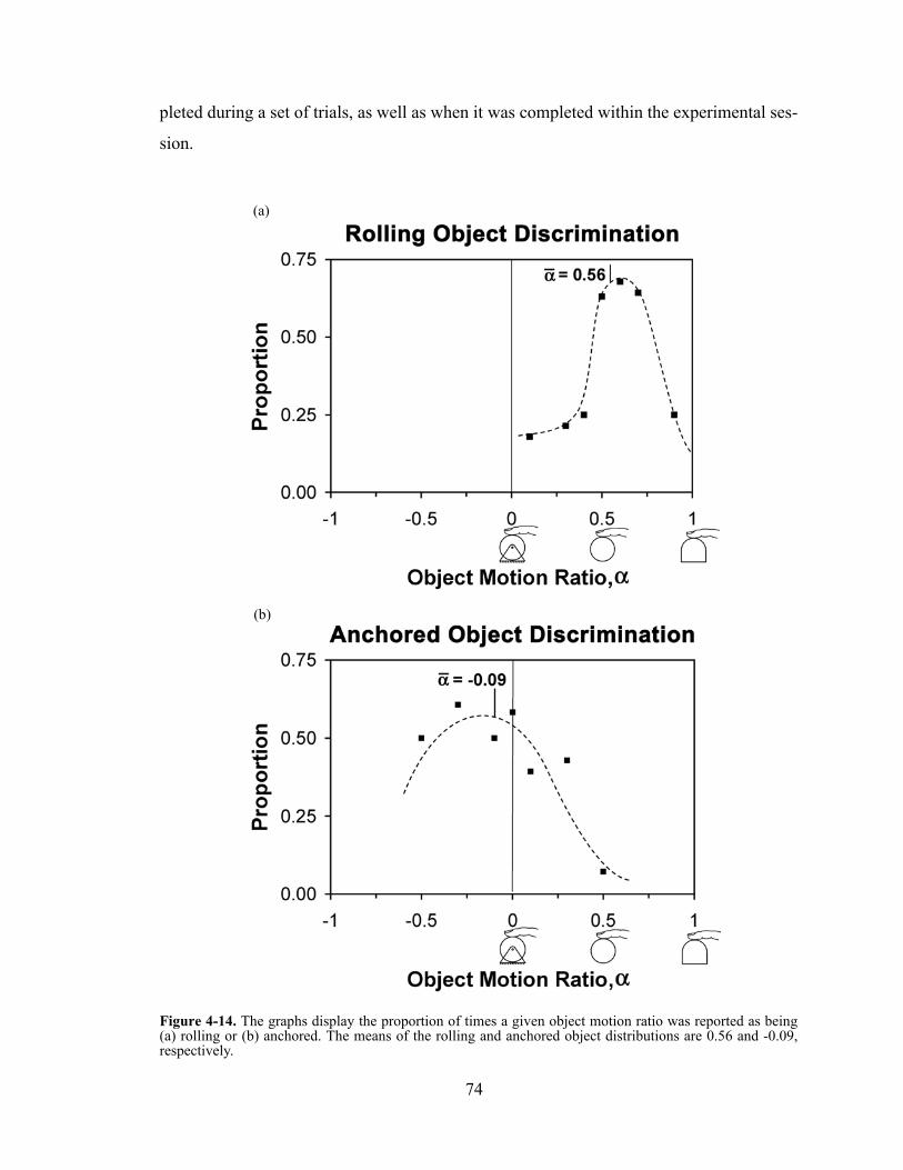
pleted during a set of trials, as well as when it was completed within the experimental ses-

sion.

Figure 4-14. The graphs display the proportion of times a given object motion ratio was reported as being (a) rolling or (b) anchored. The means of the rolling and anchored object distributions are 0.56 and -0.09, respectively.

(a)

(b)

74

The results of trials in which the motion standards (i.e., α = 0 or α = 0.5) were pre-

sented first were isolated and examined. The data were also partitioned into those trials in

which α was increasing and those in which sequential stimuli in each trial involved α

decreasing. Statistical analysis of these data revealed that the order of presentation did not

have a significant effect.

Trends in subject data were also compared from the beginning versus the end of

each set of 12 trials. There were no trends for perception of rolling objects; however, for

anchored objects, it was found that many subjects gravitated towards objects with zero or

negative α value towards the end of the set of trials. Perhaps this is because some people

simply chose objects which most restricted their motion (even if this involved actively

moving opposite to their motion).

Subject data were also partitioned into groups based on when a particular set of

trials occured. Those completing the motion experiments first were compared to those com-

pleting motion experiments at the end of the session. Those completing rolling experiments

first were also compared to those completing anchored object discriminations first. In both

cases, there was a statistical difference for judgements made of anchored objects between

the two groups. Subjects who completed anchored object discriminations later in the exper-

iments more reliably identified a truly anchored object (α ~ 0 as opposed to α ~ -0.1) com-

pared to those completing anchored discriminations first. Learning is a possible

explanation for such behavior.

Beyond the successful discrimination, subjects also commented that this experi-

ment felt realistic. These findings suggest the device forms a promising new approach to

tactile display.

4.6 General Discussion and ConclusionsThis work has presented a novel device for displaying contact centroid location during

haptic interactions. Unlike pin arrays, it is easily mounted on a traditional haptic display

and integrated with force feedback.

In controlled experiments, it was found that human subjects could easily use the

device to determine the curvature of virtual objects. Moreover, the just noticeable differ-

75

ence (JND) values obtained with the device were comparable to those obtained with phys-

ical specimens and direct finger contact. Different trends between virtual and direct contact

illustrate slightly different perception modes and lead to increased virtual discrimination

for large radii of curvature.

The virtual objects were discriminated with a Weber fraction of approximately 0.11,

indicating that users can detect changes in object radius greater than 11%. Based on the

motion of the contact point, this finding also implies a tactile length Weber fraction of 0.11.

It was also found that users of the device could identify various types of object

motion based on the contact location change, specifically discerning rolling and anchored

objects. Anecdotally, subjects reported that they found the sensation of traveling contacts a

convincing simulation and a welcome improvement over probing the virtual world with a

stylus.

76

5 Extensions and Conclusions

Through the work presented in this thesis, one only begins to understand what an exquisite

instrument the human is. It represents a significant achievement of nature that man may

never fully succeed in replicating. However, this thesis makes two small contributions to

this effort. This final chapter summarizes the work presented in chapters 3 and 4 on tactile

sensing and display, respectively. It summarizes the main contributions of this work and

suggests possible extensions and future work.

5.1 Summary of ContributionsThe major contributions of this thesis are:

• A new sensor for measuring local object geometry

This sensor is meant for use in object manipulation tasks where knowledge of local

object geometry is essential for object motion planning. In contrast to previous sen-

sors, which either infer object curvature from a nearly rigid sensing array or which

lead to complex non-linear problems, this sensor measures curvature directly. The

sensor employs standard foil strain gages and circuitry tailored to the task of mea-

suring curvature. The sensor’s half-bridge circuitry produces an output signal that

is linear with curvature and reduces sensitivity to temperature fluctuations. A math-

ematical framework was established to reconstruct the sensor geometry via an array

of curvature measurements, based on classical Fourier analysis. The sensor is ana-

lyzed and its inherent accuracy and sensitivity are determined numerically and in

experiments.

• A new approach to tactile display

This new approach is based on displaying only a single contact representative of the

centroid of contacts. Based on previous work in autonomous robotics, knowledge

77

of contact conditions is essential for robotic dexterous manipulation. The goal was

to provide a human teleoperator with this same information. A device was devel-

oped and tested on a virtual reality testbed, but is also envisioned to be used in tel-

erobotic applications.

• Evaluation of human perception of contact location feedback

Human subjects performed virtual manipulation tasks to better understand the value

of displaying contact location in addition to force feedback. Testing indicated that

subjects could easily distinguish between rolling and anchored object behaviors,

which correspond to an important state change during manipulation. Experiments

also showed that for gently curved objects, subjects’ curvature discrimination abil-

ities with the contact display device were comparable to their ability when directly

manipulating physical models (for objects about 30 mm in radius, the measured

JND was approximately 4 mm).

• Thresholds for cutaneous length-based perception, as used in rolling objects between

the fingers, were determined.

Because only a single point of contact is displayed when representing contact with

a virtual object, the judgements made in virtual curvature discrimination experi-

ments are based on the length traveled by the roller. Therefore, these tests have also

contributed cutaneous length-based JNDs, not currently available in the psycho-

physics literature. From experiments, the Weber fraction for cutaneous length based

discrimination is approximately 0.11, meaning that subjects could distinguish

between a roller travel of 5 mm and 5.55 mm.

5.2 Improvements and ExtensionsAs with most designs, one learns a great deal from each generation of prototypes. The

devices presented in this thesis have evolved considerably since their conception; however,

it is clear that many improvements can still be made. The following subsections, outline

suggested improvements and possible future work in these areas.

78

5.2.1 Tactile SensorPreliminary tests with the second-generation prototype indicate that future sensors should

be packaged to reduce the initial curvature, improving sensor performance (reducing hys-

teretic error contributions). The feasibility of combining the sensing element and electron-

ics on a single flexible substrate has been shown. However, experience suggests that it is

more practical to separate the sensing element from the sensor electronics while in the pro-

totyping stage. Sensor electronics with a suitable flex-circuit connector can be acquired

inexpensively from commercial PCB vendors, permitting rapid independent iteration of the

flexible sensing element.

The sensor performance could also be improved by modifying the way the sensor

is mounted. The initial shape of the sensor was chosen to resemble the robot fingertips cur-

rently used for dexterous manipulation (semi-circular). However, superimposing a rela-

tively high initial curvature on the sensor exacerbates sensor hysteresis and ultimately

reduces sensor accuracy. Therefore, mounting the sensor element so that its initial curvature

is reduced should improve its performance.

Results from calibration testing and thermal modeling also suggest modifying the

way the gages are affixed to the substrate. Inhomogenous bonding can lead to mechanical

hysteresis and thermal drift. Depositing sensor elements directly on a flexible substrate,

rather than bonding prefabricated gages to a flex-circuit, would dramatically reduce sensor

hysteresis and extend the dynamic range of the sensor. This would also reduce thermal gra-

dients between the gages. Adopting a substrate with higher conductivity will further

improve the sensor’s thermal stability. DuPont has developed a special formulation of poly-

imide, called KaptonTM MT that has three times the thermal conductivity of standard poly-

imide, that would be a good candidate substrate for the next generation sensor.

In addition to the above advantages, deposition and photolithography techniques

will make it possible to fabricate densely populated sensor elements and associated inter-

connects. Photolithography and deposition also provide a practical method for producing

two-dimensional arrays and vias. One issue that must be addressed when making a two-

dimensional array is the sensor’s ability to conform to complex geometries. Fabricating the

79

array on a mesh-like substrate may be a solution to this problem. Other solutions may be

found in adapting approaches from the clothing and composites industries.

5.2.2 Contact Location DisplayThe contact location display is a valuable addition to force-feedback for virtual and

remote environments. The results obtained thus far suggest that this approach will enable

users to determine object geometry and changes in contact configuration during dexterous

manipulation. The success also suggests many additional developments, including conver-

sion to two degrees of freedom for display of lateral as well as proximal/distal contact

motion. For this incarnation, the tactile element would perhaps become a ball bearing.

Other modifications may not be as straight forward. Imparting lateral motions to the tactile

element by differentially actuating push/pull wires (similar to those shown in the current

1-DOF design) seems a logical first approach. However, there are several potential issues

with this approach derived from the additional degree of freedom. One of the advantages

of the current design is that the lateral stiffness of the push-pull wires provides a passive

degree of freedom for making and breaking contact with the tactile element. For the two

degree of freedom version, it may be difficult to design a linkage with an additional degree

of freedom that will still take advantage of the passive stiffness of the push-pull wires to

prevent contact of the tactile element with the finger in free space (as shown in Figure 4-

4). Thus, it may become necessary to actively control the making and breaking of contact

(by the addition of a sensor and/or actuator). In addition, the same compliance of the push-

pull wires will also limit the lateral actuation force available to move the tactile element

laterally over the fingerpad (this was not an issue for actuation along the length of the fin-

ger, since the push-pull wires are aligned with this axis of motion). Therefore, one can see

that augmenting the current design with an additional degree of freedom represents a chal-

lenging design problem.

Other variations of the current design would be more straightforward to implement.

One might consider using a brake to control roller rotation, making it possible to transmit

shear forces through the roller similar to those experienced during sliding contact. This pro-

vides an exciting opportunity to meld the current work in contact location display with

work presented by Salada et al. [2002] on the display of slip for rendering virtual surfaces.

80

It would also be interesting to use this feature to simulate the skin stretch experienced when

sliding a finger over a surface. This could be done by building a mechanical shear model

of the finger and commanding appropriate contact positions to compensate for skin stretch

based on the direction of travel while in contact.

One might also consider specifically tailoring the design of the tactile element to

add functionality or more closely replicate specific surface properties (e.g., surface geom-

etry, stiffness, and/or friction). For example, if medical students were to use contact loca-

tion display to practice breast examinations, one might imagine constructing a tactile

element made of silicone rubber to replicate the mechanical properties of breast tissue. Per-

haps the tactile element would also include one or several internal pins to indicate possible

subdermal masses. Other designs for multifunctional tactile elements have been envisioned

in which one would place prototypical surface features around the circumference of a roller

drum, and rotate the drum to the desired position when a particular surface type is desired.

For example, a roller might have 3 positions on it that are smooth, textured and with a knife

edge to render sliding or rolling over a smooth surface, sliding over a rough surface, and

sliding along a sharp edge, respectively. Of course this type of design also necessitates addi-

tional actuation.

Ultimately, the goal is to incorporate contact location feedback in a multi-fingered

system for dexterous manipulation of virtual or remote objects. The current design can be

adapted to this end; however, there are obvious packaging issues with placing several such

devices in close proximity. The first issue is the possible mechanical (side-by-side) inter-

ference of placing thimbles on neighboring fingers. A similar interference issue occurs

when grasping virtual objects. Hardware on the pad-side of the fingers and thumb can pos-

sibly collide and/or interfere. Routing of the multiple sets of push-pull wires could also

prove challenging.

It would also be interesting to extend the current experimental investigation to

better understand what aspects of manipulation the device can best communicate. For

instance, in manipulation, the transition from rolling to sliding contact represents an impor-

tant event. One could imagine coding this event under the current kinematical framework

as continuously varying the value of α during a slip event.

81

Another feature of the device that was not specifically investigated is its ability to

make and break contact with virtual objects (as shown in Figure 4-4). Users stated that this

feature enhanced the tactile illusion of initiating new contact. However, one might also con-

sider taking this one step further. A typical complaint made of most virtual environments is

that they feel as if one is interacting with a "nerf" world. This is a result of objects rendered

as linear spring elements and a by-product of limited motor torque. Deficient torque is a

serious limitation that hinders one’s ability to render stiff interactions. However, one could

consider taking advantage of the passive degree of freedom (normal to the finger surface)

that exists between the PhantomTM and thimble. One could consider enhancing the percep-

tion of a stiff object or object impact by anticipating contact and bringing the roller into

contact with the finger with a commanded velocity designed to impede the user’s interpen-

etration into a virtual object (i.e., matched momentum haptic rendering of impact).

5.3 ConclusionThis thesis has described new methods of tactile sensing and display for dexterous dexter-

ous telemanipulation and virtual reality. A tactile sensor was developed specifically to mea-

sure local object geometry useful for manipulation planning. A companion tactile display

renders the location of the centroid of contact, an important cue about object curvature in

manipulation and exploration tasks. Concepts for both devices have been validated with

initial experiments that clearly show their potential and shed new light on the human per-

ception of curvature in manipulation tasks.

82

Appendix A: Sensor Bridge Circuitry and Thermal Modelling

This appendix gives some general background in strain gage circuitry and also presents

some results from thermal modeling of the sensor presented in chapter 3.

A.1 Strain Gage Bridge CircuitryThis section presents some basic background for strain gage bridge circuitry that is relevant

to the sensor presented in chapter 3. The goal of this sensor is to measure curvature. Since

curvature is proportional to bending strain, basic bridge equations are developed with this

goal in mind. Figure A-1 shows several configurations which can be used to measure bend-

ing strains. The main difference between these different options is the number of strain

sensing elements. The simplest possible configuration, the quarter bridge (see Figure A-

1(b)), utilizes a single strain gage on one side of the substrate, and is represented in the asso-

ciated bridge circuit by its resistance, R1. Here the remaining resistors, labeled Rd, are

simply resistors on a circuit board. Keeping the design as simple as possible is desirable.

However, there are many potential benefits to using additional gages in the bridge circuit.

Some of these benefits are listed at the bottom of Figure A-1. Most importantly, the half-

bridge and full-bridge configurations (shown in Figures A-1(c) and (d)) are temperature

compensated1 and reject axial strains, which allow bending strains to be isolated (see

Fraden [1996] as well as the comments that follow Equation A.2). Both of these properties

are essential for this sensor. In choosing between the half- and full-bridge options, the sim-

pler half-bridge configuration was chosen for the final sensor design. The half-bridge pos-

sesses the same key benefits as the full-bridge, but requires only half of the area.

1. These configurations reduce sensitivity to gross temperature fluctuations, but are still susceptible to drift when a temperature differential exists between a gage-pair, as can occur when the substrate has poor conduc-tivity. See thermal modelling results in section A.2.

83

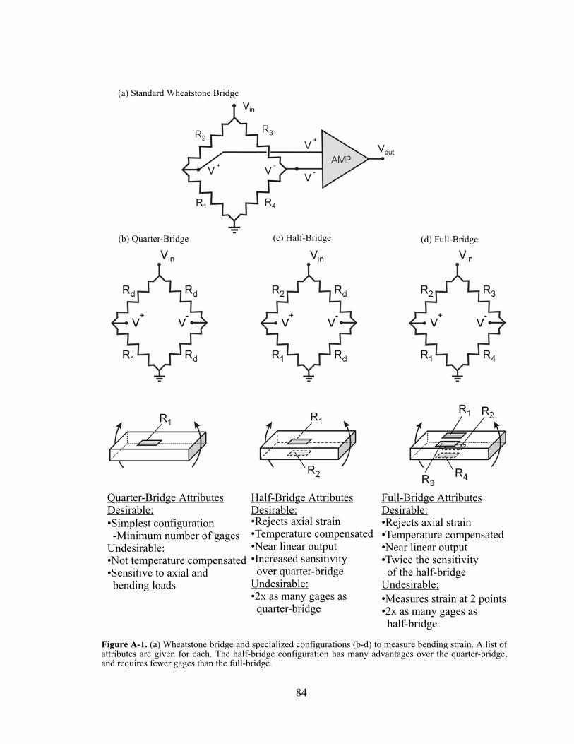
Figure A-1. (a) Wheatstone bridge and specialized configurations (b-d) to measure bending strain. A list of attributes are given for each. The half-bridge configuration has many advantages over the quarter-bridge, and requires fewer gages than the full-bridge.

(b) Quarter-Bridge (d) Full-Bridge(c) Half-Bridge

(a) Standard Wheatstone Bridge

Quarter-Bridge Attributes

•Simplest configuration

•Not temperature compensated•Sensitive to axial and

-Minimum number of gages

Half-Bridge Attributes

•Rejects axial strain

•Near linear output•Increased sensitivity

•Temperature compensated

over quarter-bridge

Full-Bridge Attributes

•Rejects axial strain

•Near linear output•Twice the sensitivity

•Temperature compensated

of the half-bridge

•Measures strain at 2 points

Desirable:

Undesirable:

Desirable:

Undesirable:•2x as many gages as quarter-bridge

Desirable:

Undesirable:

•2x as many gages as half-bridge

bending loads

84

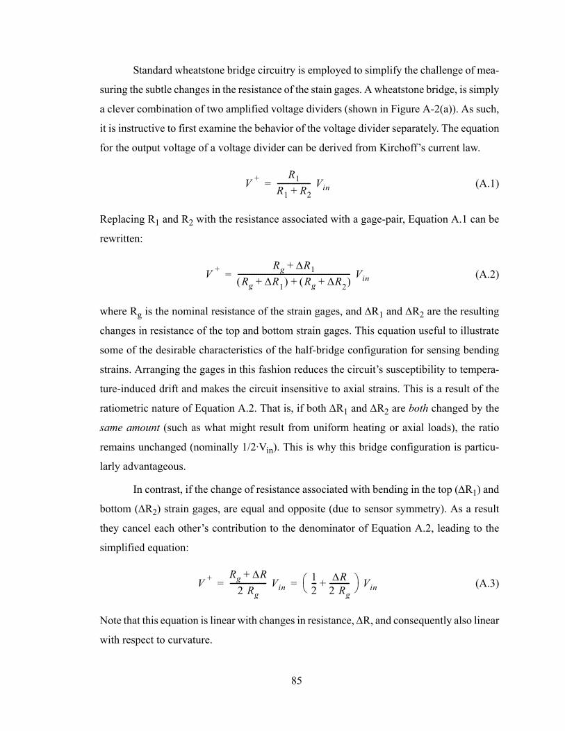
Standard wheatstone bridge circuitry is employed to simplify the challenge of mea-

suring the subtle changes in the resistance of the stain gages. A wheatstone bridge, is simply

a clever combination of two amplified voltage dividers (shown in Figure A-2(a)). As such,

it is instructive to first examine the behavior of the voltage divider separately. The equation

for the output voltage of a voltage divider can be derived from Kirchoff’s current law.

(A.1)

Replacing R1 and R2 with the resistance associated with a gage-pair, Equation A.1 can be

rewritten:

(A.2)

where Rg is the nominal resistance of the strain gages, and ∆R1 and ∆R2 are the resulting

changes in resistance of the top and bottom strain gages. This equation useful to illustrate

some of the desirable characteristics of the half-bridge configuration for sensing bending

strains. Arranging the gages in this fashion reduces the circuit’s susceptibility to tempera-

ture-induced drift and makes the circuit insensitive to axial strains. This is a result of the

ratiometric nature of Equation A.2. That is, if both ∆R1 and ∆R2 are both changed by the

same amount (such as what might result from uniform heating or axial loads), the ratio

remains unchanged (nominally 1/2·Vin). This is why this bridge configuration is particu-

larly advantageous.

In contrast, if the change of resistance associated with bending in the top (∆R1) and

bottom (∆R2) strain gages, are equal and opposite (due to sensor symmetry). As a result

they cancel each other’s contribution to the denominator of Equation A.2, leading to the

simplified equation:

(A.3)

Note that this equation is linear with changes in resistance, ∆R, and consequently also linear

with respect to curvature.

V + R1R1 R2+------------------ Vin=

V + Rg ∆R1+Rg ∆R+ 1( ) Rg ∆R+ 2( )+

------------------------------------------------------------- Vin=

V + Rg ∆R+2 Rg

-------------------- Vin 12--- ∆R

2 Rg----------- +

Vin= =

85

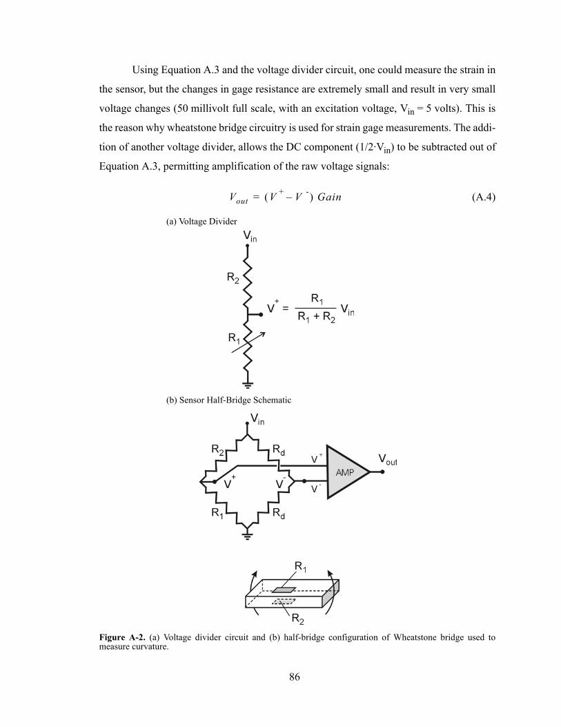
Using Equation A.3 and the voltage divider circuit, one could measure the strain in

the sensor, but the changes in gage resistance are extremely small and result in very small

voltage changes (50 millivolt full scale, with an excitation voltage, Vin = 5 volts). This is

the reason why wheatstone bridge circuitry is used for strain gage measurements. The addi-

tion of another voltage divider, allows the DC component (1/2·Vin) to be subtracted out of

Equation A.3, permitting amplification of the raw voltage signals:

(A.4)Vout V + V -–( ) Gain=

Figure A-2. (a) Voltage divider circuit and (b) half-bridge configuration of Wheatstone bridge used to measure curvature.

(b) Sensor Half-Bridge Schematic

(a) Voltage Divider

86

where V+ is unamplified half-bridge output and V - is the output of a dummy half-bridge

used to zero out the bridge circuit (nominally V- = 1/2·Vin). Substituting Equation 3.13 (the

change in resistance associated with bending strain) into Equations A.3 and A.4 yields the

final bridge equation for measuring bending strains with a pair of back-to-back gages wired

in a half-bridge configuration (shown in Figure A-2(b)):

(A.5)

where Vin is the bridge excitation voltage, rave is the mean radius of curvature of the mem-

brane centerline, ts is the thickness of the membrane substrate, tg is the gage thickness and

“Gain” is the bridge amplification. Equation A.5 can be rearranged in terms of average cur-

vature, κ, where curvature can be shown as the reciprocal of radius of curvature and κ(i)

represents the curvature of the ith gage-pair.

(A.6)

A.2 Sensor Thermal ModellingAs mentioned in section 3.3, it is important to consider thermal effects in the performance

of piezoresistive sensors such as the one presented in this thesis. A thermal model of the

sensor was developed to help understand environmental effects. This model is quite simple,

but is useful as a tool for investigating possible sources of thermally-induced imbalance in

a gage-pair of a half-bridge. This is particularly important because thermal drift is consis-

tently a major source of error in piezoresistive sensors.

A.2.1 Thermal Modelling ResultsThis section presents results that were generated using the thermal model presented in

section 3.3. Several scenarios were investigated to help understand the sensor’s sensitivity

to temperature. These models focus on predicting the differential temperature between

gages in a single gage-pair. Material properties and parameter values used to generate these

results are reported in Tables A-1 and A-2. The power input for the thermal model is

3.0 mW, which corresponds to the excitation voltage of 1.2 volts and a gage resistance of

VoutVin GF ts tg+( ) Gain⋅ ⋅⋅

4rave-------------------------------------------------------------=

κ i( ) 1rave---------=

4VoutVin GF ts tg+( ) Gain⋅ ⋅⋅-------------------------------------------------------------=

87

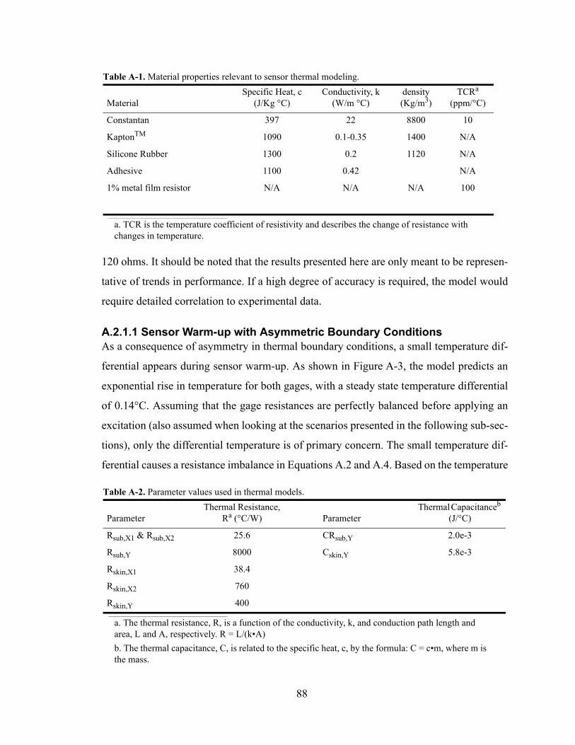
120 ohms. It should be noted that the results presented here are only meant to be represen-

tative of trends in performance. If a high degree of accuracy is required, the model would

require detailed correlation to experimental data.

A.2.1.1 Sensor Warm-up with Asymmetric Boundary ConditionsAs a consequence of asymmetry in thermal boundary conditions, a small temperature dif-

ferential appears during sensor warm-up. As shown in Figure A-3, the model predicts an

exponential rise in temperature for both gages, with a steady state temperature differential

of 0.14°C. Assuming that the gage resistances are perfectly balanced before applying an

excitation (also assumed when looking at the scenarios presented in the following sub-sec-

tions), only the differential temperature is of primary concern. The small temperature dif-

ferential causes a resistance imbalance in Equations A.2 and A.4. Based on the temperature

Table A-1. Material properties relevant to sensor thermal modeling.

MaterialSpecific Heat, c

(J/Kg °C)Conductivity, k

(W/m °C)density (Kg/m3)

TCRa (ppm/°C)

Constantan 397 22 8800 10

KaptonTM 1090 0.1-0.35 1400 N/A

Silicone Rubber 1300 0.2 1120 N/A

Adhesive 1100 0.42 N/A

1% metal film resistor N/A N/A N/A 100

a. TCR is the temperature coefficient of resistivity and describes the change of resistance with changes in temperature.

Table A-2. Parameter values used in thermal models.

ParameterThermal Resistance,

Ra (°C/W)

a. The thermal resistance, R, is a function of the conductivity, k, and conduction path length and area, L and A, respectively. R = L/(k•A)

ParameterThermal Capacitanceb

(J/°C)

b. The thermal capacitance, C, is related to the specific heat, c, by the formula: C = c•m, where m is the mass.

Rsub,X1 & Rsub,X2 25.6 CRsub,Y 2.0e-3

Rsub,Y 8000 Cskin,Y 5.8e-3

Rskin,X1 38.4

Rskin,X2 760

Rskin,Y 400

88

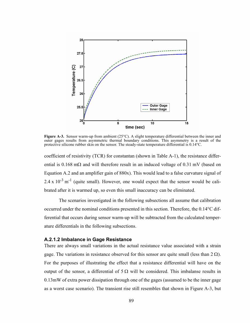
coefficient of resistivity (TCR) for constantan (shown in Table A-1), the resistance differ-

ential is 0.168 mΩ and will therefore result in an induced voltage of 0.31 mV (based on

Equation A.2 and an amplifier gain of 880x). This would lead to a false curvature signal of

2.4 x 10-3 m-1 (quite small). However, one would expect that the sensor would be cali-

brated after it is warmed up, so even this small inaccuracy can be eliminated.

The scenarios investigated in the following subsections all assume that calibration

occurred under the nominal conditions presented in this section. Therefore, the 0.14°C dif-

ferential that occurs during sensor warm-up will be subtracted from the calculated temper-

ature differentials in the following subsections.

A.2.1.2 Imbalance in Gage ResistanceThere are always small variations in the actual resistance value associated with a strain

gage. The variations in resistance observed for this sensor are quite small (less than 2 Ω).

For the purposes of illustrating the effect that a resistance differential will have on the

output of the sensor, a differential of 5 Ω will be considered. This imbalanse results in

0.13mW of extra power dissipation through one of the gages (assumed to be the inner gage

as a worst case scenario). The transient rise still resembles that shown in Figure A-3, but

Figure A-3. Sensor warm-up from ambient (25°C). A slight temperature differential between the inner and outer gages results from asymmetric thermal boundary conditions. This asymmetry is a result of the protective silicone rubber skin on the sensor. The steady-state temperature differential is 0.14°C.

89

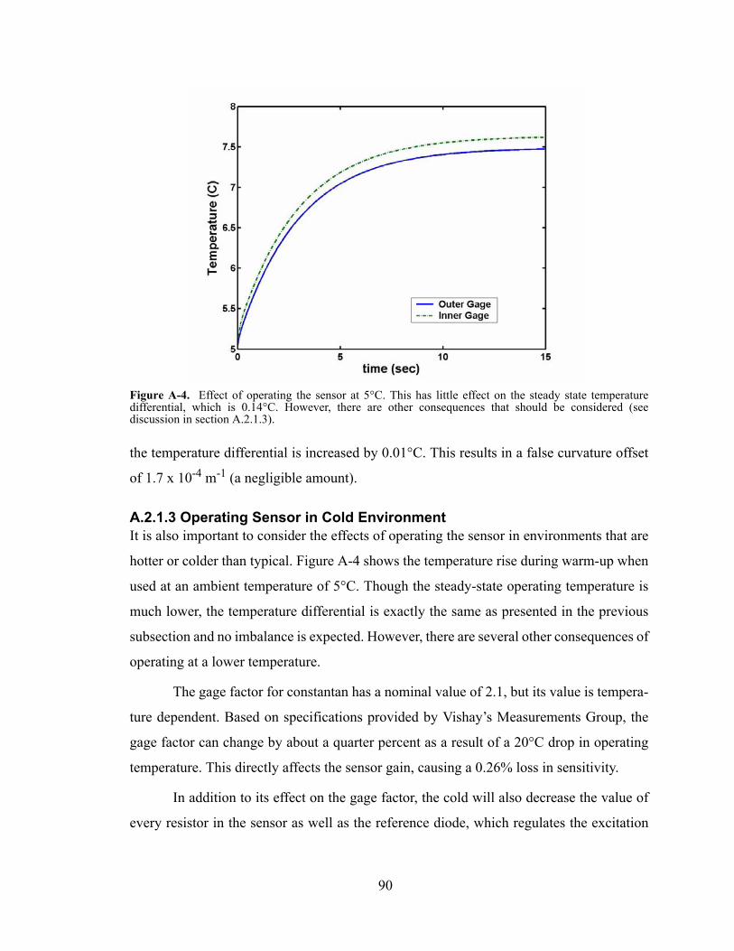
the temperature differential is increased by 0.01°C. This results in a false curvature offset

of 1.7 x 10-4 m-1 (a negligible amount).

A.2.1.3 Operating Sensor in Cold EnvironmentIt is also important to consider the effects of operating the sensor in environments that are

hotter or colder than typical. Figure A-4 shows the temperature rise during warm-up when

used at an ambient temperature of 5°C. Though the steady-state operating temperature is

much lower, the temperature differential is exactly the same as presented in the previous

subsection and no imbalance is expected. However, there are several other consequences of

operating at a lower temperature.

The gage factor for constantan has a nominal value of 2.1, but its value is tempera-

ture dependent. Based on specifications provided by Vishay’s Measurements Group, the

gage factor can change by about a quarter percent as a result of a 20°C drop in operating

temperature. This directly affects the sensor gain, causing a 0.26% loss in sensitivity.

In addition to its effect on the gage factor, the cold will also decrease the value of

every resistor in the sensor as well as the reference diode, which regulates the excitation

Figure A-4. Effect of operating the sensor at 5°C. This has little effect on the steady state temperature differential, which is 0.14°C. However, there are other consequences that should be considered (see discussion in section A.2.1.3).

90

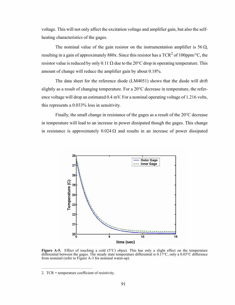
voltage. This will not only affect the excitation voltage and amplifier gain, but also the self-

heating characteristics of the gages.

The nominal value of the gain resistor on the instrumentation amplifier is 56 Ω,

resulting in a gain of approximately 880x. Since this resistor has a TCR2 of 100ppm/°C, the

resistor value is reduced by only 0.11 Ω due to the 20°C drop in operating temperature. This

amount of change will reduce the amplifier gain by about 0.18%.

The data sheet for the reference diode (LM4051) shows that the diode will drift

slightly as a result of changing temperature. For a 20°C decrease in temperature, the refer-

ence voltage will drop an estimated 0.4 mV. For a nominal operating voltage of 1.216 volts,

this represents a 0.033% loss in sensitivity.

Finally, the small change in resistance of the gages as a result of the 20°C decrease

in temperature will lead to an increase in power dissipated though the gages. This change

in resistance is approximately 0.024 Ω and results in an increase of power dissipated

2. TCR = temperature coefficient of resistivity.

Figure A-5. Effect of touching a cold (5°C) object. This has only a slight effect on the temperature differential between the gages. The steady state temperature differential is 0.17°C, only a 0.03°C difference from nominal (refer to Figure A-3 for nominal warm-up).

91

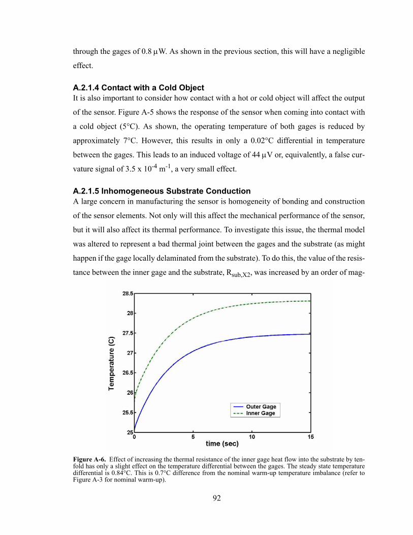
through the gages of 0.8 µW. As shown in the previous section, this will have a negligible

effect.

A.2.1.4 Contact with a Cold ObjectIt is also important to consider how contact with a hot or cold object will affect the output

of the sensor. Figure A-5 shows the response of the sensor when coming into contact with

a cold object (5°C). As shown, the operating temperature of both gages is reduced by

approximately 7°C. However, this results in only a 0.02°C differential in temperature

between the gages. This leads to an induced voltage of 44 µV or, equivalently, a false cur-

vature signal of 3.5 x 10-4 m-1, a very small effect.

A.2.1.5 Inhomogeneous Substrate ConductionA large concern in manufacturing the sensor is homogeneity of bonding and construction

of the sensor elements. Not only will this affect the mechanical performance of the sensor,

but it will also affect its thermal performance. To investigate this issue, the thermal model

was altered to represent a bad thermal joint between the gages and the substrate (as might

happen if the gage locally delaminated from the substrate). To do this, the value of the resis-

tance between the inner gage and the substrate, Rsub,X2, was increased by an order of mag-

Figure A-6. Effect of increasing the thermal resistance of the inner gage heat flow into the substrate by ten-fold has only a slight effect on the temperature differential between the gages. The steady state temperature differential is 0.84°C. This is 0.7°C difference from the nominal warm-up temperature imbalance (refer to Figure A-3 for nominal warm-up).

92

nitude (altering Rsub,X2 represents the worst case scenario). As shown in Figure A-6, this

leads to an additional temperature differential between the gages of 0.7°C, an induced volt-

age of 1.54 mV or, equivalently, a false curvature signal of 0.012 m-1. This makes a much

larger contribution than many of the other sources of thermal imbalance.

A.2.2 Summary of Thermal Modelling ResultsThe simple thermal model presented herein makes a useful tool for examining thermal

effects for this sensor. In agreement with actual sensor behavior, the model predicts a small

temperature rise during warm-up that is on order of a few degrees. In examining the sce-

narios presented in section A.2.1, there are three main design factors that greatly affect the

sensor’s ability to maintain relative immunity to thermal effects. These factors are: (1) the

conductivity of the substrate (Rsub,Y), (2) bonding of the substrate to the gages (Rsub,X), and

(3) thermal isolation provided by a protective skin (Rskin,X2).

The most important design factor is the substrate. The substrate must have good

thermal conduction in order to dissipate heat and reduce temperature gradients between the

gages. In addition, it is also extremely important that the thermal interface between the sub-

strate and gages is homogeneous. Slight variations, or worse, a partial delamination can

lead to temperature differentials that can induce spurious signals of considerable magni-

tude. The third of these factors is the insulating protective skin, such as the silicone rubber

skin chosen for the sensor. The protective skin reduces heat transfer from the environment

and thus reduces internal thermal gradients.

Contributions of the most significant thermal effects are listed in Table 3-2.

93

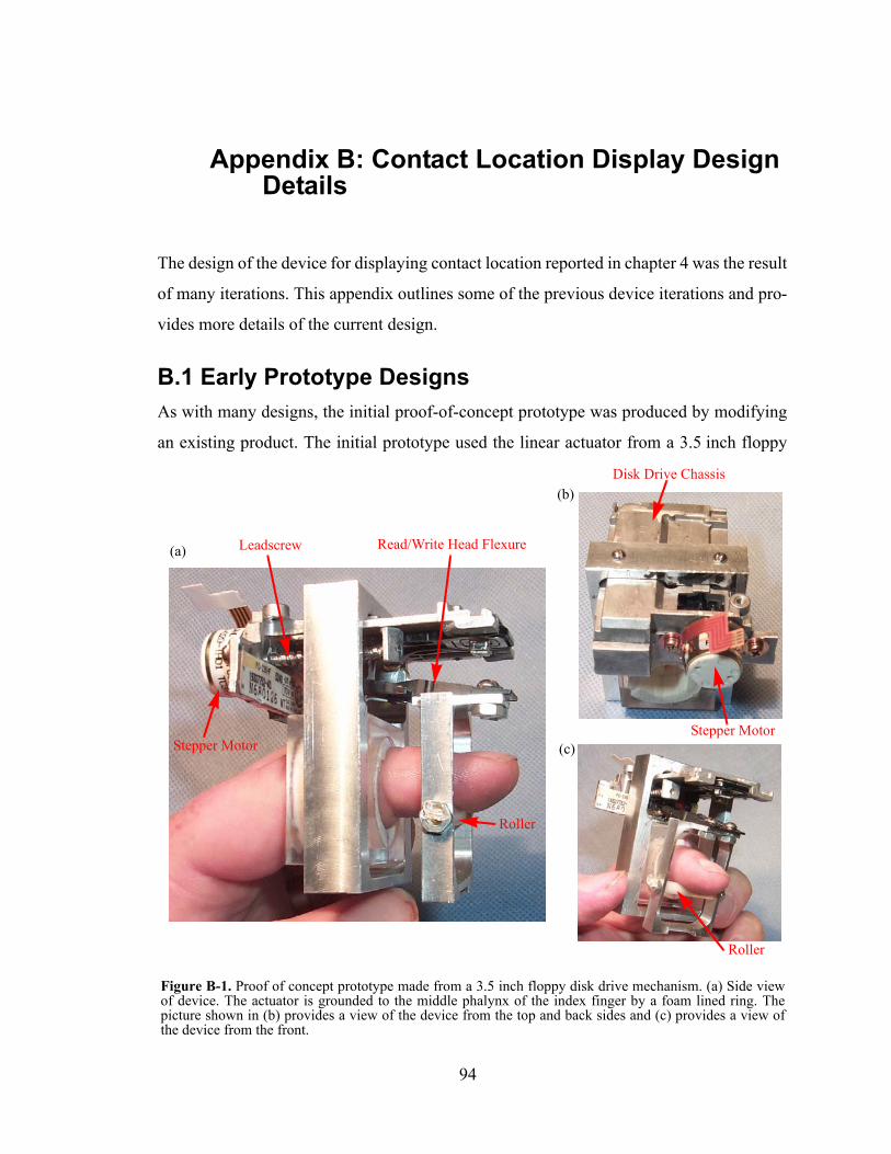
Appendix B: Contact Location Display Design Details

The design of the device for displaying contact location reported in chapter 4 was the result

of many iterations. This appendix outlines some of the previous device iterations and pro-

vides more details of the current design.

B.1 Early Prototype DesignsAs with many designs, the initial proof-of-concept prototype was produced by modifying

an existing product. The initial prototype used the linear actuator from a 3.5 inch floppy

Figure B-1. Proof of concept prototype made from a 3.5 inch floppy disk drive mechanism. (a) Side view of device. The actuator is grounded to the middle phalynx of the index finger by a foam lined ring. The picture shown in (b) provides a view of the device from the top and back sides and (c) provides a view of the device from the front.

(a)

(b)

(c)Stepper Motor

Read/Write Head Flexure

Roller

Disk Drive Chassis

Stepper Motor

Roller

Leadscrew

94

disk drive. Figure B-1(b) shows the portion of the disk drive chassis that was cut away from

the rest of the disk drive, leaving only the portion necessary to support the linear actuator

mechanism. A simple bracket was designed to mount the actuator to the middle phalynx of

the index finger, and a small bracket was used to suspend a small roller off the arm origi-

nally used to support the read/write head. A small torsion spring on the arm supporting the

read/write head provided a preload force to keep the roller in contact with the user’s finger

as it flexed or extended. The disk drive’s bipolar stepper motor provided a simple means to

drive the motion of the actuator (using a standard stepper motor driver chip like a

MC3479); however, pulses of the stepper motor produce a buzzing sensation that rapidly

numb the receptors of the user’s fingertip. Other issues included somewhat clumsy ergo-

nomics and insufficient motor torque that caused the actuator to lose steps. Despite these

issues, this prototype did demonstrate the potential of displaying contact location, and soon

after its completion, work began on a custom-designed device that would address the short-

comings of this simple prototype.

The subsequent design (see Figure B-2) was also mounted to the middle phalynx of

the index finger (a second unit was also envisioned for the thumb to permit use with the

lab’s two-fingered telemanipulator). This device was designed to fit a wide range of finger

sizes. This was accomplished by designing the device such that it could be mated and

demated to interchangeable rings that could be custom designed to the dimensions of the

user’s finger. This interface also provided a natural pivot for the device that is coincident

with the axis of rotation of the distal interphalangeal joint. This pivot provides a degree of

freedom for the roller to follow the contour of the finger as it is flexed or extended during

manipulation tasks. It also provides a degree of freedom to make and break contact with the

user’s finger. It was envisioned that the device would be used in combination with Immer-

sion’s CyberGrasp. A torsion spring provides a small moment that moves the roller away

from the user’s fingertip (see Figure B-2(a)). Force applied through the cables of the Cyber-

Grasp counteracts the moment of the spring and brings the roller into contact with the fin-

ger.

Like the design presented in chapter 4, this device employs a linear actuator to posi-

tion a small roller along the user's fingertip. The device is grounded to the finger using a

95

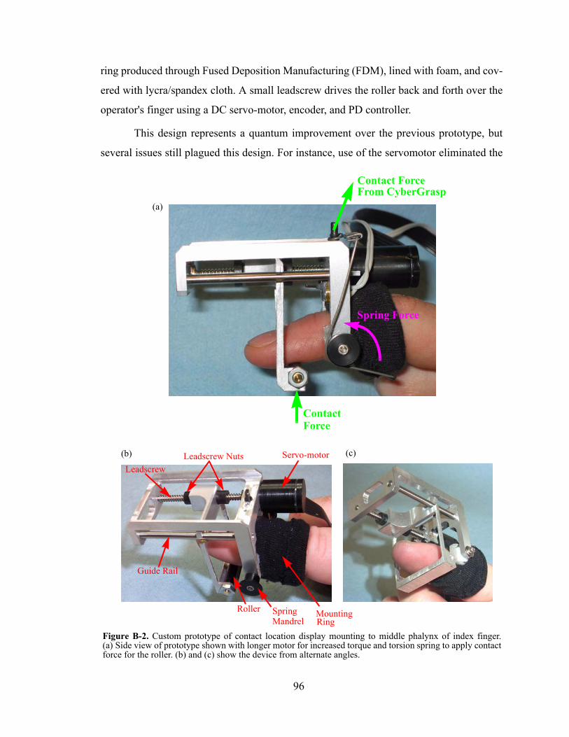
ring produced through Fused Deposition Manufacturing (FDM), lined with foam, and cov-

ered with lycra/spandex cloth. A small leadscrew drives the roller back and forth over the

operator's finger using a DC servo-motor, encoder, and PD controller.

This design represents a quantum improvement over the previous prototype, but

several issues still plagued this design. For instance, use of the servomotor eliminated the

Figure B-2. Custom prototype of contact location display mounting to middle phalynx of index finger. (a) Side view of prototype shown with longer motor for increased torque and torsion spring to apply contact force for the roller. (b) and (c) show the device from alternate angles.

(a)

(b) (c)

Roller

LeadscrewLeadscrew Nuts

Guide Rail

Spring

Servo-motor

MountingRing

Contact ForceFrom CyberGrasp

Spring Force

Mandrel

ContactForce

96

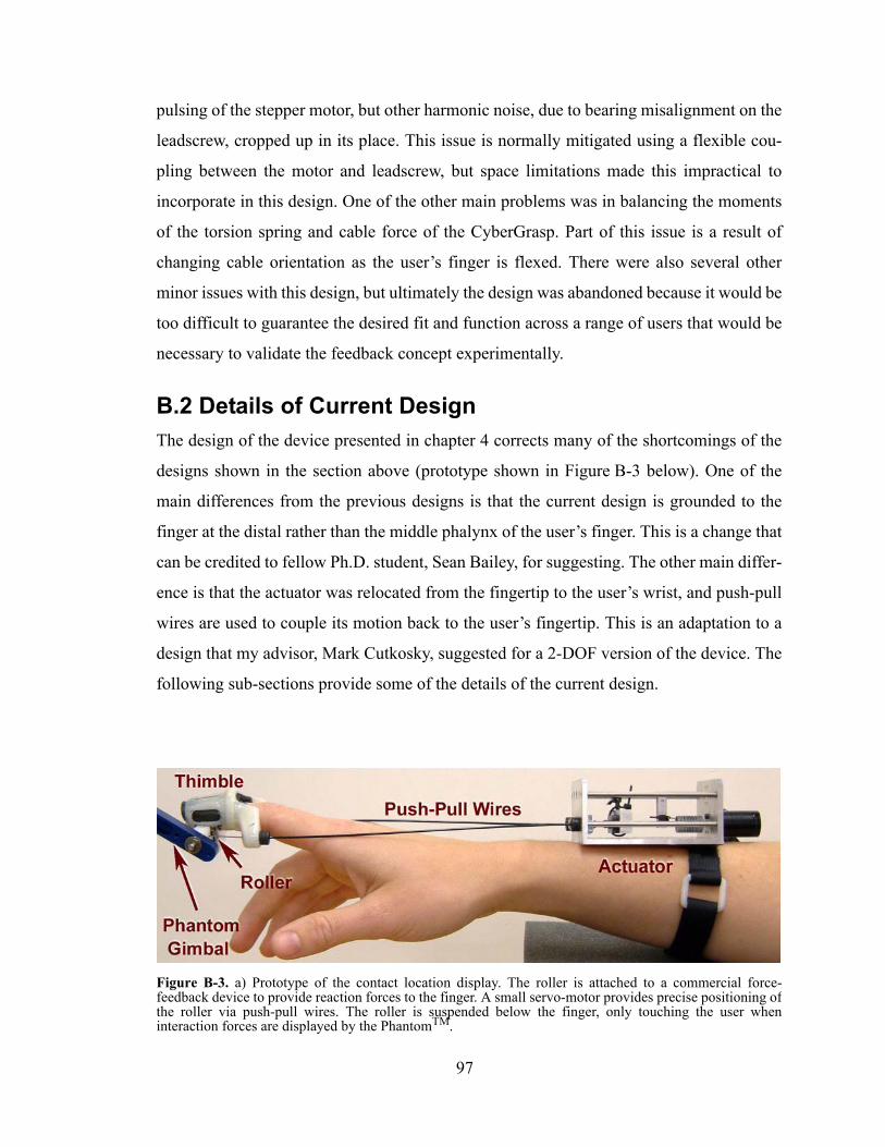
pulsing of the stepper motor, but other harmonic noise, due to bearing misalignment on the

leadscrew, cropped up in its place. This issue is normally mitigated using a flexible cou-

pling between the motor and leadscrew, but space limitations made this impractical to

incorporate in this design. One of the other main problems was in balancing the moments

of the torsion spring and cable force of the CyberGrasp. Part of this issue is a result of

changing cable orientation as the user’s finger is flexed. There were also several other

minor issues with this design, but ultimately the design was abandoned because it would be

too difficult to guarantee the desired fit and function across a range of users that would be

necessary to validate the feedback concept experimentally.

B.2 Details of Current DesignThe design of the device presented in chapter 4 corrects many of the shortcomings of the

designs shown in the section above (prototype shown in Figure B-3 below). One of the

main differences from the previous designs is that the current design is grounded to the

finger at the distal rather than the middle phalynx of the user’s finger. This is a change that

can be credited to fellow Ph.D. student, Sean Bailey, for suggesting. The other main differ-

ence is that the actuator was relocated from the fingertip to the user’s wrist, and push-pull

wires are used to couple its motion back to the user’s fingertip. This is an adaptation to a

design that my advisor, Mark Cutkosky, suggested for a 2-DOF version of the device. The

following sub-sections provide some of the details of the current design.

Figure B-3. a) Prototype of the contact location display. The roller is attached to a commercial force-feedback device to provide reaction forces to the finger. A small servo-motor provides precise positioning of the roller via push-pull wires. The roller is suspended below the finger, only touching the user when interaction forces are displayed by the PhantomTM.

97

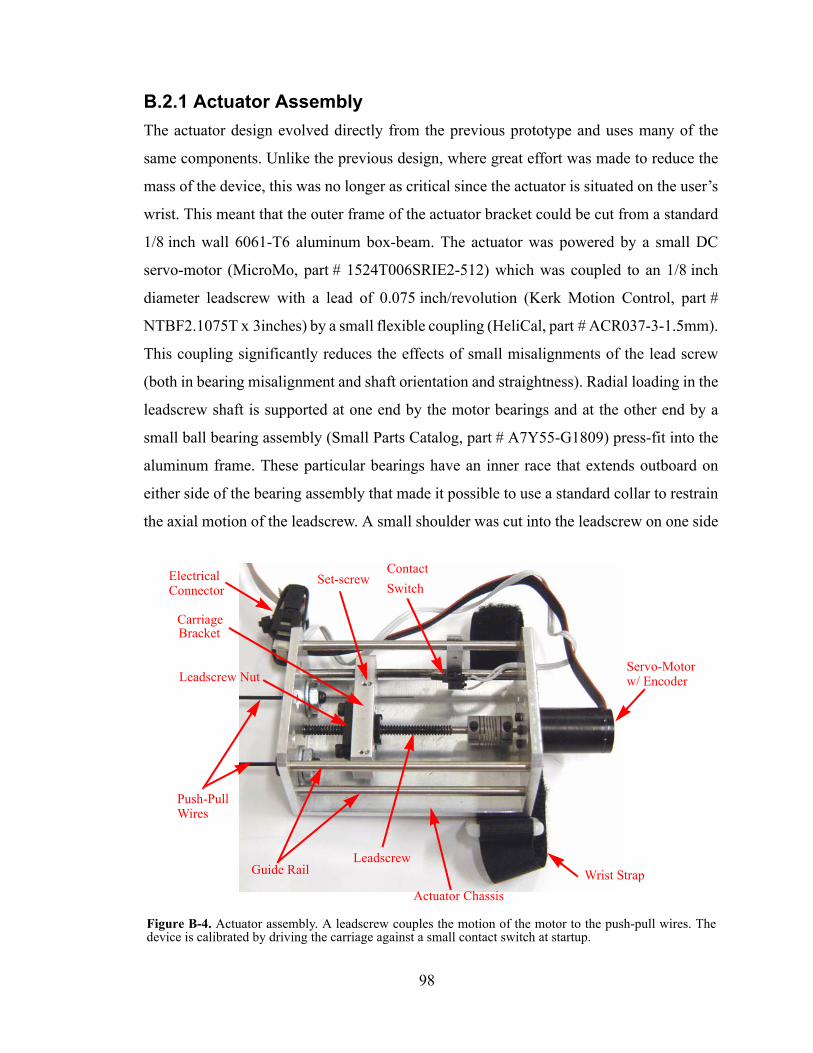
B.2.1 Actuator AssemblyThe actuator design evolved directly from the previous prototype and uses many of the

same components. Unlike the previous design, where great effort was made to reduce the

mass of the device, this was no longer as critical since the actuator is situated on the user’s

wrist. This meant that the outer frame of the actuator bracket could be cut from a standard

1/8 inch wall 6061-T6 aluminum box-beam. The actuator was powered by a small DC

servo-motor (MicroMo, part # 1524T006SRIE2-512) which was coupled to an 1/8 inch

diameter leadscrew with a lead of 0.075 inch/revolution (Kerk Motion Control, part #

NTBF2.1075T x 3inches) by a small flexible coupling (HeliCal, part # ACR037-3-1.5mm).

This coupling significantly reduces the effects of small misalignments of the lead screw

(both in bearing misalignment and shaft orientation and straightness). Radial loading in the

leadscrew shaft is supported at one end by the motor bearings and at the other end by a

small ball bearing assembly (Small Parts Catalog, part # A7Y55-G1809) press-fit into the

aluminum frame. These particular bearings have an inner race that extends outboard on

either side of the bearing assembly that made it possible to use a standard collar to restrain

the axial motion of the leadscrew. A small shoulder was cut into the leadscrew on one side

Figure B-4. Actuator assembly. A leadscrew couples the motion of the motor to the push-pull wires. The device is calibrated by driving the carriage against a small contact switch at startup.

Wrist StrapLeadscrew

Leadscrew Nut

Guide Rail

Actuator Chassis

Servo-Motor

Set-screwElectricalConnector

ContactSwitch

w/ Encoder

Push-PullWires

CarriageBracket

98

of the bearing to restrain motion along the length of the leadscrew in one direction, while

the collar captures motion in the opposite direction so that axial loads are carried through

the press-fit bearing rather than the motor bearings.

The rotary motion of the motor is converted to linear motion using a standard

flanged leadscrew nut (Kerk Motion Control, part # BF2.1075N) that is in turn bolted to an

aluminum carriage bracket. This bolted interface permitted easy interchanging of different

pitch leadscrew/nut combinations for fine tuning device performance. The carriage bracket

couples the linear travel of the leadscrew nut to the two push-pull wires. The connection to

the leadscrew shaft locks down all but the rotational degree of freedom (about the lead-

screw shaft) of the carriage bracket. This degree of freedom is restrained by 1/8 inch diam-

eter polished guide rail on which a machined slot in the carriage bracket rests.

Small 0-80 set-screws were used to lock the position of the push-pull wires to the

carriage bracket, allowing easy adjustment of the push-pull wires. The push-pull wire

assemblies were grounded to the actuator chassis by a threaded (10-32) interface. External

machine nuts were used to fasten this interface rather than threading the through-hole in the

chassis (or using nut plates) because the wire assemblies needed to be free to rotate to

permit interchanging of thimbles. Because of this arrangement, one only needs to loosen

these nuts when interchanging thimbles.

A small contact switch is used to calibrate the actuator encoders upon startup. This

switch is mounted to a small bracket whose position can be adjusted along the length of the

1/8 inch diameter guide rails. The switch, although compact, has a relatively long 0.1 inch

stroke before bottoming out. Consequently, there are no hard collisions during calibration.

The switch was scavenged from an old HP floppy drive.

99

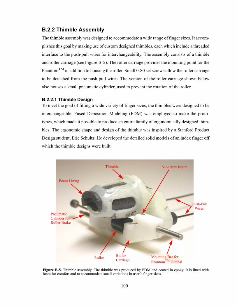
B.2.2 Thimble AssemblyThe thimble assembly was designed to accommodate a wide range of finger sizes. It accom-

plishes this goal by making use of custom designed thimbles, each which include a threaded

interface to the push-pull wires for interchangeability. The assembly consists of a thimble

and roller carriage (see Figure B-5). The roller carriage provides the mounting point for the

PhantomTM in addition to housing the roller. Small 0-80 set screws allow the roller carriage

to be detached from the push-pull wires. The version of the roller carriage shown below

also houses a small pneumatic cylinder, used to prevent the rotation of the roller.

B.2.2.1 Thimble DesignTo meet the goal of fitting a wide variety of finger sizes, the thimbles were designed to be

interchangeable. Fused Deposition Modeling (FDM) was employed to make the proto-

types, which made it possible to produce an entire family of ergonomically designed thim-

bles. The ergonomic shape and design of the thimble was inspired by a Stanford Product

Design student, Eric Schultz. He developed the detailed solid models of an index finger off

which the thimble designs were built.

Figure B-5. Thimble assembly. The thimble was produced by FDM and coated in epoxy. It is lined with foam for comfort and to accommodate small variations in user’s finger sizes.

Roller

Thimble

Foam Lining

Pneumatic

Mounting Bar for

Set-screw Insert

Push-PullWires

PhantomTM Gimbal

Cylinder forRoller Brake

RollerCarriage

100

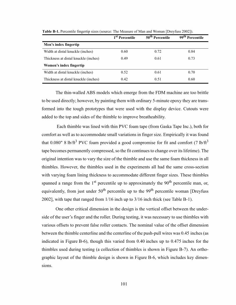
The thin-walled ABS models which emerge from the FDM machine are too brittle

to be used directly; however, by painting them with ordinary 5-minute epoxy they are trans-

formed into the tough prototypes that were used with the display device. Cutouts were

added to the top and sides of the thimble to improve breatheability.

Each thimble was lined with thin PVC foam tape (from Gaska Tape Inc.), both for

comfort as well as to accommodate small variations in finger size. Empirically it was found

that 0.080" 8 lb/ft3 PVC foam provided a good compromise for fit and comfort (7 lb/ft3

tape becomes permanently compressed, so the fit continues to change over its lifetime). The

original intention was to vary the size of the thimble and use the same foam thickness in all

thimbles. However, the thimbles used in the experiments all had the same cross-section

with varying foam lining thickness to accommodate different finger sizes. These thimbles

spanned a range from the 1st percentile up to approximately the 90th percentile man, or,

equivalently, from just under 50th percentile up to the 99th percentile woman [Dreyfuss

2002], with tape that ranged from 1/16 inch up to 3/16 inch thick (see Table B-1).

One other critical dimension in the design is the vertical offset between the under-

side of the user’s finger and the roller. During testing, it was necessary to use thimbles with

various offsets to prevent false roller contacts. The nominal value of the offset dimension

between the thimble centerline and the centerline of the push-pull wires was 0.45 inches (as

indicated in Figure B-6), though this varied from 0.40 inches up to 0.475 inches for the

thimbles used during testing (a collection of thimbles is shown in Figure B-7). An ortho-

graphic layout of the thimble design is shown in Figure B-6, which includes key dimen-

sions.

Table B-1. Percentile fingertip sizes (source: The Measure of Man and Woman [Dreyfuss 2002]).1st Percentile 50th Percentile 99th Percentile

Men’s index fingertip

Width at distal knuckle (inches) 0.60 0.72 0.84

Thickness at distal knuckle (inches) 0.49 0.61 0.73

Women’s index fingertip

Width at distal knuckle (inches) 0.52 0.61 0.70

Thickness at distal knuckle (inches) 0.42 0.51 0.60

101

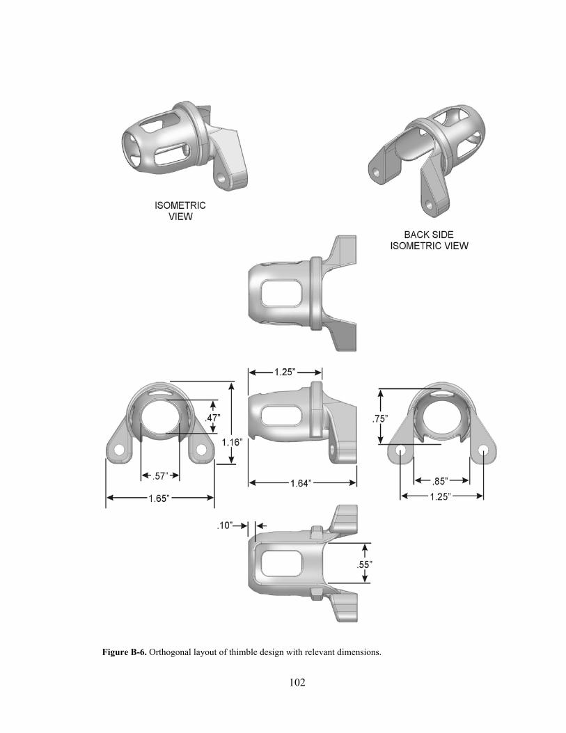
Figure B-6. Orthogonal layout of thimble design with relevant dimensions.

102

B.2.3 Push-Pull Wire AssembliesThe push-pull wire assemblies work much like the brake and shifter cables on a bicycle.

However, instead of stranded steel cable, the present design uses solid spring wire to pre-

vent buckling during pushing motions. Several options for the push-pull wire assemblies

were considered. Each of these designs were similar, utilizing steel spring wire with a plas-

tic jacket, with either end of the plastic jacket terminated by center-drilled socket head cap

screws. Terminating these assemblies with a standard threaded interface permitted initial

fine tuning of the wire assemblies and interchangeability of thimbles to accommodate a

wide range of finger sizes. The threaded interface also simplified device maintenance.

Initially, standard nylon-jacketed assemblies from Carl Stahl Sava Industries, Inc.

were considered (eg., part # C-130N which includes a 0.032 inch diameter stainless steel

wire and 0.130 inch O.D. nylon sheath). This drove the initial sizing of the threaded inter-

face which terminates the wire assemblies. It was determined that a 10-32 cap screw would

be required for the 0.130 inch diameter hole which would accommodate the nylon sheaths.

Conveniently, the nylon sheaths were stiff enough to be press-fit into the cap screws with-

out restricting the motion of the internal wires. However, there was a small problem with

these wire assemblies. Their large diameter made them very stiff, which required the user

to overcome the inherent stiffness of the push-pull sheaths when flexing their finger.

Figure B-7. A family of thimbles were used to accommodate the wide range of finger sizes. The thimbles are lined with 1/6 inch, 1/8 inch, or 3/16 inch PVC foam tape. The thimbles also differ based on the vertical offset from the bottom of the user’s finger to the centerline of the push-pull wires.

103

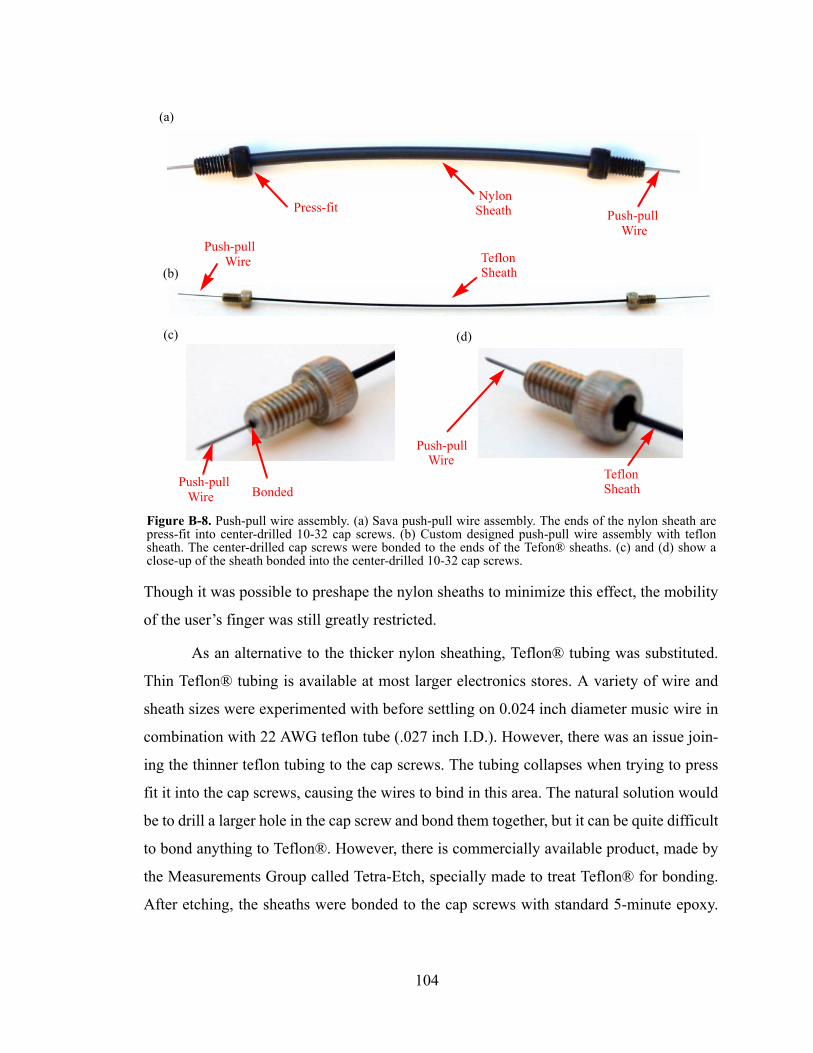
Though it was possible to preshape the nylon sheaths to minimize this effect, the mobility

of the user’s finger was still greatly restricted.

As an alternative to the thicker nylon sheathing, Teflon® tubing was substituted.

Thin Teflon® tubing is available at most larger electronics stores. A variety of wire and

sheath sizes were experimented with before settling on 0.024 inch diameter music wire in

combination with 22 AWG teflon tube (.027 inch I.D.). However, there was an issue join-

ing the thinner teflon tubing to the cap screws. The tubing collapses when trying to press

fit it into the cap screws, causing the wires to bind in this area. The natural solution would

be to drill a larger hole in the cap screw and bond them together, but it can be quite difficult

to bond anything to Teflon®. However, there is commercially available product, made by

the Measurements Group called Tetra-Etch, specially made to treat Teflon® for bonding.

After etching, the sheaths were bonded to the cap screws with standard 5-minute epoxy.

Figure B-8. Push-pull wire assembly. (a) Sava push-pull wire assembly. The ends of the nylon sheath are press-fit into center-drilled 10-32 cap screws. (b) Custom designed push-pull wire assembly with teflon sheath. The center-drilled cap screws were bonded to the ends of the Tefon® sheaths. (c) and (d) show a close-up of the sheath bonded into the center-drilled 10-32 cap screws.

(a)

(b)

(c)

NylonPress-fit

Bonded

(d)

Sheath

TeflonSheath

TeflonSheath

Push-pullWire

Push-pullWire

Push-pullWire

Push-pullWire

104

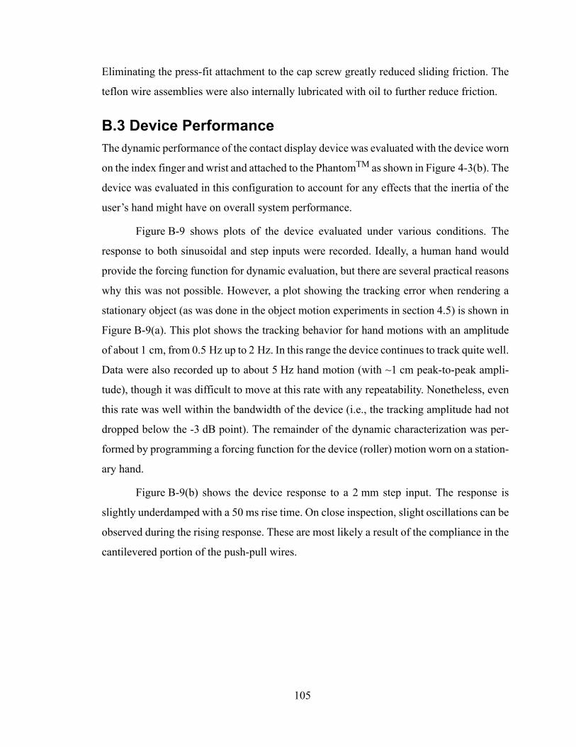
Eliminating the press-fit attachment to the cap screw greatly reduced sliding friction. The

teflon wire assemblies were also internally lubricated with oil to further reduce friction.

B.3 Device PerformanceThe dynamic performance of the contact display device was evaluated with the device worn

on the index finger and wrist and attached to the PhantomTM as shown in Figure 4-3(b). The

device was evaluated in this configuration to account for any effects that the inertia of the

user’s hand might have on overall system performance.

Figure B-9 shows plots of the device evaluated under various conditions. The

response to both sinusoidal and step inputs were recorded. Ideally, a human hand would

provide the forcing function for dynamic evaluation, but there are several practical reasons

why this was not possible. However, a plot showing the tracking error when rendering a

stationary object (as was done in the object motion experiments in section 4.5) is shown in

Figure B-9(a). This plot shows the tracking behavior for hand motions with an amplitude

of about 1 cm, from 0.5 Hz up to 2 Hz. In this range the device continues to track quite well.

Data were also recorded up to about 5 Hz hand motion (with ~1 cm peak-to-peak ampli-

tude), though it was difficult to move at this rate with any repeatability. Nonetheless, even

this rate was well within the bandwidth of the device (i.e., the tracking amplitude had not

dropped below the -3 dB point). The remainder of the dynamic characterization was per-

formed by programming a forcing function for the device (roller) motion worn on a station-

ary hand.

Figure B-9(b) shows the device response to a 2 mm step input. The response is

slightly underdamped with a 50 ms rise time. On close inspection, slight oscillations can be

observed during the rising response. These are most likely a result of the compliance in the

cantilevered portion of the push-pull wires.

105

In contrast to Figure B-9(a), the plots in (c) and (d) were generated by driving the

roller with a sinusoid with the user’s hand stationary. A plot of the tracking performance

when driven by a 5 Hz sine wave with 1 cm peak-to-peak amplitude is shown in Figure B-

9(c). A similar plot for a 8 Hz sine wave is shown in Figure B-9(d). Tracking performance

degrades significantly in going from 5 Hz up to 8 Hz, where it reaches the -3dB point. From

these plots, it was determined that the small motion bandwidth of the device is approxi-

mately 8 Hz.

Figure B-9. Performance plots for the contact display device. (a) Tracking plot for the device rendering a stationary object. The desired position is based on the motion of the user’s finger. (b) Device response to a 2 mm step input. The response is slightly underdamped with a 50 ms rise time. In contrast to (a) plots (c) and (d) were generated by driving the roller with a sinusoid with the user’s hand stationary. (c) Tracking plot for the contact display driven by a 5 Hz sine wave with 1 cm peak-to-peak amplitude. (d) Tracking plot for the contact display driven by a 8 Hz sine wave with 1 cm peak-to-peak amplitude. As seen in plot (d), there is considerable lag as the tracking performance falls off. The small motion bandwidth of the device is approximately 8 Hz. Plots shown courtesy of Katherine J. Kuchenbecker of the Stanford Telerobotics Lab.

(a) (b)

(c) (d)

106

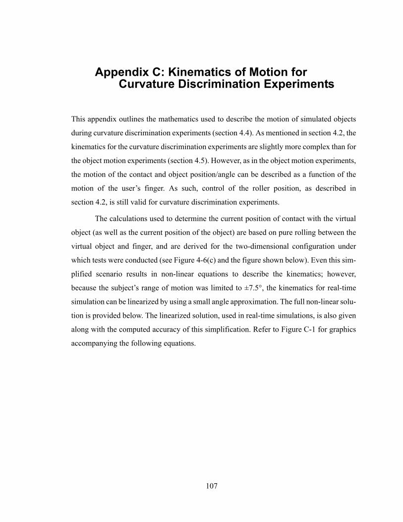
Appendix C: Kinematics of Motion for Curvature Discrimination Experiments

This appendix outlines the mathematics used to describe the motion of simulated objects

during curvature discrimination experiments (section 4.4). As mentioned in section 4.2, the

kinematics for the curvature discrimination experiments are slightly more complex than for

the object motion experiments (section 4.5). However, as in the object motion experiments,

the motion of the contact and object position/angle can be described as a function of the

motion of the user’s finger. As such, control of the roller position, as described in

section 4.2, is still valid for curvature discrimination experiments.

The calculations used to determine the current position of contact with the virtual

object (as well as the current position of the object) are based on pure rolling between the

virtual object and finger, and are derived for the two-dimensional configuration under

which tests were conducted (see Figure 4-6(c) and the figure shown below). Even this sim-

plified scenario results in non-linear equations to describe the kinematics; however,

because the subject’s range of motion was limited to ±7.5°, the kinematics for real-time

simulation can be linearized by using a small angle approximation. The full non-linear solu-

tion is provided below. The linearized solution, used in real-time simulations, is also given

along with the computed accuracy of this simplification. Refer to Figure C-1 for graphics

accompanying the following equations.

107

The position and motion of the point of contact, P, and the orientation, θ, of the vir-

tual object can be described as a function of the horizontal motion of the user’s finger, ∆XF.

The following equation describes the initial position of the point of contact, P1.

(C.1)

where Rd is the distance from the origin (the pivot point) to the center of curvature for each

stimulus, rc is the radius of this disk, and θ1 is the orientation of the virtual object at time 1.

Rd can always be determined from Rw and rc, because the curves of the stimuli are inscribed

in a circular wheel of radius, Rw. Thus,

(C.2)

Figure C-1. Schematic representation of the virtual object motion in curvature discrimination experiments. Virtual objects were constrained to follow an arc, pivoting about the origin. The curvature stimuli were small circular disks inscribed on a circular wheel of radius, Rw. Only x and y motions of the virtual finger were allowed (no rotation), so object kinematics can be described purely as a function of finger position, given some initial configuration.

P1 Rd θ1sin( ) ex Rd θ1 rc+cos( ) ey+–=

Rd Rw rc–=

108

The position at some arbitrary time later, P2, can be represented similarly.

(C.3)

where θ2 is the orientation of the virtual object at time 2, and the other variables are the

same as described for Equation C.1.

Because pure rolling between the finger and the virtual object was prescribed in the

kinematic model, the motion of the user’s finger can be used to calculate the motion of the

virtual object. This allows the simulation to be driven based on measurements of the current

location of the user’s finger. For pure rolling, the arc-length over which the position of the

contact moves on both the finger and object is the same and is described by the equation.

(C.4)

In this simplified case, the contact is always on the top of the object (since the virtual finger

is not allowed to rotate), so the position of the user’s finger in the x-direction at time 2

(XF,2) can be related to the final position of the object using the relation in Equation C.4.

(C.5)

The following equation relates the user’s finger motion to the motion of the contact and

object.

(C.6)

This equation can be rewritten in terms of the initial orientation and the unknown rotation

of the wheel.

(C.7)

Rewriting this in a suitable form to solve for the unknown rotation angle, ∆θ, using standard

trigonometric identities.

(C.8)

P2 Rd θ2sin( ) ex Rd θ2 rc+cos( ) ey+–=

∆s rc ∆θ=

XF 2, P2 ex⋅ ∆s– R– d θ2sin rc ∆θ–= =

∆XF XF 2, XF 1,– R– d θ2sin rc ∆θ–( ) R– d θ1sin( )–= =

∆XF Rd θ1sin θ1 ∆θ+( )sin–( ) rc ∆θ–=

∆XF Rd θ1sin θ1 ∆cos θ ∆θ θ1cossin+sin( )–[ ] rc ∆θ–=

109

Rearranging Equation C.8 results in an equation in terms of the previously computed stim-

ulus angle, θ1, other known constants, and the finger motion in the x-direction, ∆XF.

(C.9)

The y-position of the contact and user’s finger can be described similarly. While in

contact, the change in y-position of the user’s finger and the y-position of the contact is

identical and is simply a function of the unknown wheel rotation, as is the case for the x-

direction shown in Equation C.9.

(C.10)

So, if Equation C.9 can be solved for the rotation of the stimulus, ∆θ, the position

of the contact and virtual object can be fully described. A standard numerical approach to

solving a nonlinear equation, such as Equation C.9, is to use Newton’s Method (also known

as Newton-Raphson). The standard form applied to solve for the change in object orienta-

tion is:

(C.11)

where ∆θi+1 is the iterated solution for ∆θ, ∆θi is the initial guess at the solution for ∆θ, and

f is simply Equation C.9 rewritten by moving ∆XF to the right hand side of the equation.

f ’ is the derivative of f

In each iteration, f is evaluated at ∆θi. The solution converges quite rapidly with a suitable

initial guess at the solution (see discussion later in this appendix for a suitable initial guess

for this solution).

In contrast to the non-linear solution, if the motions of the virtual object will only

deviate a small distance from vertical, a small-angle approximation can be applied to Equa-

tion C.9, resulting in an equation linear in ∆θ:

(C.12)

∆XF Rd θ1 1 ∆cos θ–( )sin θ1 ∆sin θcos–[ ] rc ∆θ–=

∆YF Rd θ2cos θ1cos–( ) Rd θ1 ∆θ+( )cos θ1cos–( )= =

∆θi 1+ ∆θi

f ∆θ( ) ∆θi

f ′ ∆θ( ) ∆θi

--------------------------–=

f Rd θ1 1 ∆cos θ–( )sin θ1 ∆sin θcos–[ ] rc ∆θ ∆XF––=

f ′ Rd θ1 ∆sin θsin θ1 ∆cos θcos–[ ] rc–=

∆XF Rd θ1 rc–cos–( ) ∆θ=

110

This equation can be rearranged to directly solve for ∆θ:

(C.13)

Note that for small angles the denominator of the above equation is nearly constant. This

quantity represents the instantaneous radius of rotation, and, as one can see from Equation

C.2, the denominator is nearly equal to the radius of the wheel, Rw (negated). Thus, a good

initial guess, ∆θi, for the non-linear solution of Equation C.11 is .

In the curvature discrimination experiments discussed in section 4.4, the motion of

the virtual objects was restricted to approximately ±7.5° of rotation. In these experiments,

the radius of the wheel, Rw, was 75 mm. When comparing the solutions of Equation C.11

and Equation C.13 at the extremes of travel, it is seen that there is only a slight difference.

For instance, for a finger motion 1 cm from top-dead-center and a stimulus with radius, rc,

equal to 10 mm, the linearized solution gives a net object rotation of -0.1334 radians (or -

7.643°) as opposed to the solution from the full non-linear solution of -0.1337 radians (or

-7.660°). While the linearized solution underpredicts the rotation by about 0.2% and results

in an error in rendered contact location of approximately 0.02 mm, this amount of error is

imperceptible (based on the results reported in chapter 4).

It is also interesting to compare the accuracy of the linearized solution to the accu-

racy of the PhantomTM measurements used to drive our simulation. The joint angles of the

PhantomTM are measured using 1000-tick encoders (in quadrature). In combination with

the 10:1 gear reduction of the capstan drive and link length of 15 cm, this means that 1 bit

of resolution on the encoders is equivalent to about 0.023 mm. Quite coincidentally, this is

similar to the worst-case accuracy of the linearized solution. For this reason, the linearized

equation was used in real-time computations.

∆θ∆XF

Rd θ1 rc–cos–( )--------------------------------------- =

∆θi ∆– XF Rw⁄ =

111

Bibliography

Asamura, N., Yokoyama, N., and Shinoda, H., "Selectively Stimulating Skin Receptors for Tactile Display", Computer Graphics and Applications, IEEE, vol. 18, 1998, pp. 32-37.

Asamura, N., Shinohara T., Tojo Y., Koshida N., and Shinoda H., "Necessary Spatial Res-olution for Realistic Tactile Feeling Display." In Proceedings of the 2001 Interna-tional Conference on Robotics and Automation, IEEE, 2001, pp. 1851-1856.

Bicchi, A., Salisbury, J.K., Brock, D.L., "Contact Sensing From Force Measurements." International Journal of Robotics Research 12(3), 1993 , pp. 249-262.

Biggs, J. and Srinivasan M.A., Chapter 5 in Haptic Interfaces. Handbook of Virtual Envi-ronments. K. Stanney, Ed.: London, Lawrence Earlbaum, Inc., 2002.

Brocket, R.W., "Robotic Hands with Rheological Surfaces." Proceedings of the 1985 IEEE International Conference on Robotics and Automation, 1985, pp. 942-946.

Burdea, G.C., Force and Touch Feedback for Virtual Reality. New York: J. Wiley & Sons, 1996.

Caldwell, D.G., Tsagarakis, N., Giesler, C., "An Integrated Tactile/Shear Feedback Array for Stimulation of Finger Mechanoreceptor," Proceedings of the 1999 IEEE Interna-tional Conference on Robotics and Automation, 1999, pp. 287-292.

Canepa, G.M., M., De Rossi, D., Caiti, A., Parisini, T., "Shape from Touch by a Neural Net." presented at Robotics and Automation, 1992. Proceedings., 1992 IEEE Inter-national Conference on Robotics and Automation, 1992.

Chang, D.C., "Tactile Array Sensors and Data Interpretation for Dexterous Robotic Roll-ing Manipulation." Ph.D. Thesis in Mechanical Engineering: Stanford University, 1995.

Charlebois, M.G., K.; Payandeh, S., "Shape Description of General, Curved Surfaces Using Tactile Sensing and Surface Normal Information." Proceedings of the 1997 International Conference on Robotics and Automation, IEEE, 1997, pp. 2819-2824.

Cohn, M.B., Lam, M., and Fearing, R.S., ``Tactile Feedback for Teleoperation'', SPIE Conf. 1833, Telemanipulator Technology, Boston, MA, Nov. 15-16, 1992.

112

Dario P., Tactile Sensing: Technology And Applications. Sensors And Actuators A-Physi-cal 26(1-3), 1991 pp. 251-256.

Dennerlein, J.T., Millman P.A., and Howe R.D., "Vibrotactile Feedback for Industrial Telemanipulators." Proceedings of the ASME Dynamic Systems and Control Divi-sion, Dallas, TX, USA, 1997.

Dreyfuss, H., Tilley, A.R., The Measure of Man and Woman: Human Factors in Design, New York, N.Y. : Wiley, 2002.

Fearing, R.S., Tactile Sensing, Perception and Shape Interpretation, Ph.D. Thesis in Elec-trical Engineering: Stanford University, 1988.

Fearing, R.S. and Binford T.O., "Using a Cylindrical Tactile Sensor for Determining Cur-vature." IEEE Transactions on Robotics and Automation, vol. 7, 1991, pp. 806-817.

Fearing, R.S., Moy G., and Tan E., "Some Basic Issues in Teletaction." In Proceedings of the 1997 International Conference on Robotics and Automation, IEEE, 1997, pp. 3093-3099.

Ferrier, N.J. and Brockett, R.W., "Reconstructing the Shape of a Deformable Membrane from Image Data." International Journal of Robotics Research 19(9), 2000, pp. 795-816.

Fischer, H., Neisius, B., and Trapp, R., "Tactile Feedback for Endoscopic Surgery." In Interactive Technology and New Paradign for Healthcare, edited by K. Morgan, R.M. Satava, H.B. Sieburg, R. Mattheus, J.P. Christensen,IOS Press, 1995, pp. 114-117.

Fraden, J., Handbook of Modern Sensors. 2nd edition Springer-Verlag, New York, 1996.

Fukuda, T., Morita, H., Arai, F., Ishihara, H., and Matsuura, H., "Micro Resonator Using Electromagnetic Actuator for Tactile Display." Proceedings of the 1997 Interna-tional Symposium on Micromechatronics and Human Science, 1997, pp. 143-148.

Gescheider, G.A., "Psychophysics: The Fundamentals." 3rd ed: Lawrence Erlbaum Asso-ciates, 1997.

Ghodssi, R., Beebe, D.J., White, V., Denton, D.D., "Development of a Tangential Tactor Using a Liga/MEMS Linear Microactuator Technology." International Mechanical Engineering Congress and Exposition, Microelectromechanical Systems, DSC Vol. 59, Nov. 17-22, 1996, pp. 379-386.

Goodwin, A.W., John K.T., and Marceglia A.H., "Tactile Discrimination of Curvature by Humans Using Only Cutaneous Information from the Fingerpads." Experimental Brain Research, vol. 86, 1991, pp. 663-672.

113

Gordon, I.E. and Morison V., "The Haptic Perception of Curvature." Perception & Psy-chophysics, vol. 31, 1982, pp. 446-450.

Haidacher, S. and Hirzinger G., "Contact Point Identification in Multi-Fingered Grasps Exploiting Kinematic Constraints." presented at Proceedings of the 2002 IEEE International Conference on Robotics and Automation, Washington, DC, 2002, pp. 1597 -1603.

Hasser, C.J. and Weisenberger J.M., "Preliminary Evaluation of a Shape-Memory-Alloy Tactile Feedback Display." presented at Proc. of Symposium on Haptic Interfaces for Virtual Environments and Teleoperator Systems, ASME Winter Annual Meet-ing, 1993, pp. 73–80.

Hasser, C.J. and Daniels, M.W. "Tactile Feedback with Adaptive Controller for a Force-Reflecting Haptic Display." 15th Souther Biomedical Engineering Conference, Day-ton, OH, March29-31, 1996, pp. 526-533.

Hayward, V. and Cruz-Hernandez J.M., "Tactile Display Device Using Distributed Lateral Skin Stretch," presented at Symposium on Haptic Interfaces for Virtual Environ-ment and Teleoperator Systems" , IMECE 2000, 2000.

Hogan, N. “Impedance control - An approach to manipulation: Part I. Theory.” Journal of Dynamic Systems, Measurement, and Control - Transactions of the ASME, Volume 107, Issue 1, 1985, pages 1-7.

Howe, R.D. Kontarinis, D.A.; Peine, W.J., "Shape memory alloy actuator controller design for tactile displays," Proceedings of the 34th IEEE Conference on Decision and Control, 1995, pp. 3540-3544 .

Iwata, H.Y., H.; Kawamura, R., Nakaizumi, F; Kawamura, R, "Project Feelex: Adding Haptic Surface to Graphics," presented at Proceedings of SIGGRAPH 2001, 2001.

Johansson, R.S., "How is grasping modified by somatosensory input?" In Motor Control: Concepts and Issues. Dahlem Konferenzen Edited by HUMPHREY DR, FREUND H-J, John Wiley & Sons Ltd, Chichester, 1991, pp. 331-355.

Johansson, R.S. and LaMotte, R.H., "Tactile detection thresholds for a single asperity on an otherwise smooth surface," Somatosensory Research, vol. 1(1), 1983, pp. 21-31.

Johansson, R.S. and Vallbo, Å.B., "Tactile sensory coding in the glabrous skin of the human hand," Trends Neuroscience vol. 6, 1983, pp. 27-31.

Kaczmarek, K.A. and Bach-Y-Rita, P., "Tactile Displays." In W. Barfield and T. Furness, editors, Advanced Interface Design and Virtual Environments. Oxford University Press, 1993.

114

Kaczmarek, K.A., Webster, J.G., Bach-Y-Rita, P., and Tompkins, W.J., "Electrotactile and Vibrotactile Displays for Sensory Substitution Systems." IEEE Transactions on Biomedical Engineering, vol. 38, 1991, pp. 1-16.

Kammermeier, P., Buss, M., and Schmidt, G., "Dynamic Display of Distributed Tactile Shape Information by a Prototypical Actuator Array." Proceedings of the Interna-tional Conference on Intelligent Robots and Systems, 2000, pp. 1119-1124.

Kammermeier, P. and Schmidt, G., "Application-Specific Evaluation of Tactile Array Dis-plays for the Human Fingertip," Proceedings of the International Conference on Intelligent Robots and Systems, 2002, pp. 2937-2942.

Kappers, K.M.L., Koenderink, J.J., Lichtenegger, I., "Haptic Identification of Curved Sur-faces." Perception and Psychophysics, Vol. 56(#1), July 1994, pp. 53-61.

Klatzky, R.L., & Lederman, S.J., "Intelligent exploration by the human hand." In S. Ven-kataraman & T. Iberall (Eds.), Dextrous hands for robots. New York: SpringerVer-lag, 1990, .pp. 66-81.

Kontarinis, D.A., Son J.S., Peine W.J., and Howe R.D., "A Tactile Shape Sensing and Dis-play System for Teleoperated Manipulation." Proceedings of the 1995 IEEE Interna-tional Conference on Robotics and Automation, Nagoya, Japan, May 1995, pp. 641-646.

Kontarinis, D.A. and Howe, R.D., Tactile Display of Vibratory Information in Teleopera-tion and Virtual Environments, Presence-Teleoperaotrs and Virtual Environments, vol. 4, 1995, pp. 387-402. [Kontarinis 1995a]

Lederman, S.J. "The perception of surface roughness by active and passive touch." Bulle-tin of the Psychonomic Society, 18(5), (1981), pp. 253-255.

Lee, M.H., "Tactile Sensing: New Directions, New Challenges." International Journal of Robotics Research, vol. 19, 2000, pp. 636-43.

Loomis, J.M., and Lederman, S.J. "Tactual Perception." In Boff, K.R., Kaufman, L., and Thomas, J.P. (Eds.), Handbook of perception and human performance: Vol. 2. Cong-nitive processes and performance. New York: Wiley, 1986, pp. 31.1-31.41.

Louw, S., Kappers, A.M.L, Koenderink, J.J., "Active Haptic Detection and Discrimination of Shape." Perception and Psychophysics, Vol. 64(#7), Oct. 2002, pp. 1108-1119.

Maeno, T., "Tactile Sensation of Humans - Mechanical Dynamics, Analogy and Illusion." Transactions of the Institute of Electrical Engineers of Japan, Part E, vol. 122, 2002, pp. 469-73.

115

Monkman, G.J., "Electrorheological Tactile Display." Pressence, MIT Press, Vol. 1, No. 2, 1992.

Montana, D.J., "The Kinematics of Contact and Grasp." International Journal of Robotics Research, vol. 7(3), 1988, pp. 17-32.

Moy, G., Wagner, C., and Fearing, R.S. (2000a), "A Compliant Tactile Display for Teletac-tion." IEEE Int. Conf. on Robotics and Automation, April 2000, 2000, pp. 3409-3415.

Moy, G., Singh, U., Tan, E., and Fearing, R.S. (2000b), "Human Tactile Spatial Sensitivity for Tactile Feedback," In Proceedings of the 2000 International Conference on Robotics and Automation, IEEE, 2000.

Nowlin, W.C., Experimental "Results on Bayesian Algorithms for Interpreting Compliant Tactile Sensing Data." Proceedings of the 1991 IEEE International Conference on Robotics and Automation, 1991, pp. 378-383.

Pawluk, D.T.V., Van Buskirk C.P., Killebrew J.H., Hsiao S.S., and Johnson K.O., "Control and Pattern Specification for a High Density Tactile Array." In Proceedings of the ASME Dyn. Sys. and Control Division, ASME International Mechanical Engineer-ing Congress and Exposition, New York, NY, USA, 1998, pp. 97-102.

Peine, W.J., Wellman, P.S., and Howe, R.D., "Temporal bandwidth requirements for tac-tile shape displays." Sixth Annual Symposium on Haptic Interfaces for Virtual Envi-ronment and Teleoperator Systems, ASME International Mechanical Engineering Congress and Exposition, Dallas, Nov. 15-21, 1997, pp. 107-113.

Petriu, E.M., Das S.R., Yeung S.K., Liu S.-Q., Huang W.-Y., Wang A.-M., and Song A.-G., "Robotic Tactile Perception: Overview and Prospect of Research and Development on Robot Tactile Sensory Technology", Robot, vol. 24, 2002, pp. 362-74.

Johnson K.O. and Phillips J.R., "Tactile spatial resolution: I. Two-point discrimination, gap detection, grating resolution, and letter recognition," Journal of Neurophysiol-ogy, vol. 46, 1981, pp. 1177-1191.

Rucci, M. and Dario P., "Development of Cutaneo-Motor Coordination in an Autonomous Robotic System." Autonomous Robots, vol. 1, 1994, pp. 93-106.

Russell, R.A., "A Tactile Sensor Skin for Measuring Surface Contours." IEEE TENCON 1, 1992, pp 262 -266.

Salada, M.A., Colgate J.E., Lee M.V., and Vishton P.M., "Validating a Novel Approach to Rendering Fingertip Contact Sensations." In Proceedings of the 10th Symposium on Haptic Interfaces for Virtual Environment and Teleoperator Systems, 2002, pp. 217-224.

116

Schiff, W. and Foulke, E., editors. Tactual Perception: A Sourcebook, Cambridge Univer-sity Press, Cambridge, 1982.

Sheridan, T.B. Telerobotic, Automation, and Human Supervisory Control. Cambridge, MA: The MIT Press, 1992.

Shimoga, K.B., "A Survey of Perceptual Feedback Issues in Dexterous Telemanipulation: Part I, Finger Force Feedback," Proceedings of IEEE Virtual Reality Annual Inter-national Symposium, 1993, pp. 263-270.

Shimoga, K.B., "A Survey of Perceptual Feedback Issues in Dexterous Telemanipulation: Part II, Finger Touch Feedback." Proceedings of IEEE Virtual Reality Annual Inter-national Symposium, 1993, pp. 271-279.

Shimoga, K.B. and Goldenberg A.A., Soft Robotic Fingertips. I. A Comparison of Con-struction Materials, International Journal of Robotics Research, vol. 15, 1996, pp. 320-350.

Shimojo, M., "Tactile Sensing and Display." Transactions of the Institute of Electrical Engineers of Japan, Part E, vol. 122, 2002, pp. 465-468.

Siegel, M., "Tactile Display Development: The Driving-Force for Tactile Sensor Develop-ment," presented at Haptic Virtual Environments and Their Applications, IEEE International Workshop 2002 HAVE, 2002, pp. 115-118.

Springer, S.L. and Ferrier N.J., "Design and Control of a Force-Reflecting Haptic Inter-face for Teleoperational Grasping." Journal of Mechanical Design, vol. 124, 2002, pp. 277-283.

Srinivasan, M.A. and R.H. LaMotte, "Encoding of shape in the responses of cutaneous mechanoreceptors. Information Processing in the Somatosensory System. Wenner-Gren Intl. Symposium Series. O. Franzen and J. Westman, Macmillan Press, 1991, pp. 59-69.

Summers, I.R. and Chanter C.M., "A Broadband Tactile Array on the Fingertip." Journal of the Acoustical Society of America, vol. 112, 2002, pp. 2118-2126.

Tachi, S., "Roles of Tactile Display in Virtual Reality." Transactions of the Institute of Electrical Engineers of Japan, Part E, vol. 122, 2002, pp. 461-464.

Tang, H. and Beebe D.J., "A Microfabricated Electrostatic Haptic Display for Persons with Visual Impairments." Rehabilitation Engineering, IEEE Transactions on [see also IEEE Trans. on Neural Systems and Rehabilitation], vol. 6, 1998, pp. 241-248.

117

Taylor, P.M., Creed, A.J., Sianaki, A.H., Varley, C.J., and Moser, A., "Creating the Illusion of Shape for Virtual Environments." in Innovative Actuators for Mechatronic Sys-tems, IEE Colloquium on, 1995, pp. 7/1-7/7.

Timoshenko S.P. and Gere J.M., Theory of Elastic Stability. McGraw-Hill, 1961, pp. 340-342.

Vallbo, Å.B. and Johansson, R.S., "Properties of cutaneous mechanoreceptors in the human hand related to touch sensation," Human Neurobiology, vol. 3, 1984, pp. 3-14.

Voyles, R.M. Jr., Fedder G., and Khosla P.K., "Design of a Modular Tactile Sensor and Actuator Based on an Electrorheological Gel," Proceedings of the 1996 IEEE Inter-national Conference on Robotics and Automation, 1996, pp. 13-17.

Wagner, C.R., Lederman, S.J., Howe, R.D., "A Tactile Shape Display Using Rc Servomo-tors," Proceedings of the 10th Symposium on Haptic Interfaces for Virtual Environ-ment and Teleoperator Systems, (HAPTICS 2002), 2002, pp. 354-355.

Wellman, P.S., Peine W.J., Favalora G., and Howe R.D., "Mechanical Design and Control of a High-Bandwidth Shape Memory Alloy Tactile Display." Experimental Robotics V, vol. 232, 1998, pp. 56-66.

Yoshikawa, T. and Nagura A., "A Three-Dimensional Touch/Force Display System for Haptic Interface." In Proceedings of the 1999 IEEE International Conference on Robotics and Automation, 1999, pp. 2943-2951.

Zilles, C.B. and Salisbury, J.K., "A Constraint-Based God-Object Method for Haptic Dis-play," In proceedings of the 1995 IEEE/RSJ International Conference on Intelligent Robots and Systems 95. 'Human Robot Interaction and Cooperative Robots', 1995, pp. 146-151.

118