On Stiffness in Affine Asset Pricing Models By Shirley J. Huang and Jun Yu University of Auckland & Singapore Management University

On Stiffness in Affine Asset Pricing Models

By Shirley J. Huang and Jun YuUniversity of Auckland &

Singapore Management University

Outline of Talk

Motivation and literature Stiffness in asset pricing Simulation results Conclusions

Motivation and Literature

Preamble:

“…around 1960, things became completely different and everyone became aware that world was full of stiff problems…” Dahlquist (1985)


When valuing financial assets, one often needs to find the numerical solution to a partial differential equation (PDE); see Duffie (2001).

In many practically relevant cases, for example, when the number of states is modestly large, solving the PDE is computationally demanding and even becomes impractical.


Computational burden is heavier for econometric analysis of continuous-time asset pricing models

Reasons:

1. Transition density are solutions to PDEs which have to be solved numerically at every data point and at each iteration of the numerical optimizations when maximizing likelihood (Lo;1988).

2. Asset prices themselves are numerical solutions to PDEs.


The computational burden in asset pricing and financial econometrics has prompted financial economists & econometricians to look at the class of affine asset pricing models where the risk-neutral drift and volatility functions of the process for the state variable(s) are all affine (i.e. linear).


Examples:

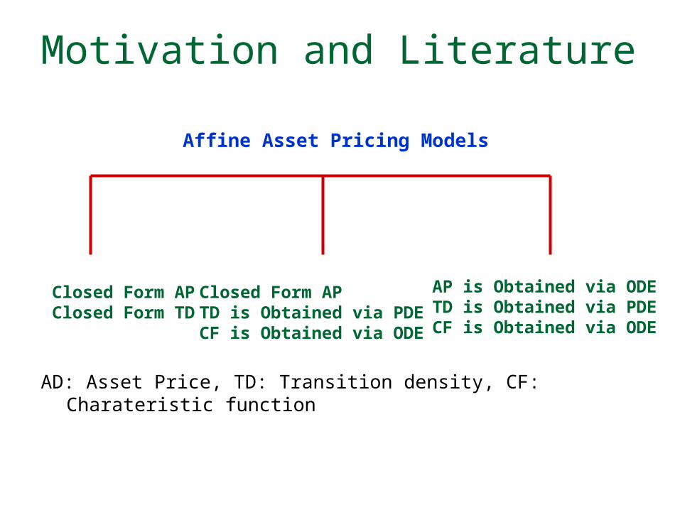
1. Closed form expression for asset prices or transition densities:

Black and Scholes (1973) for pricing equity options Vasicek (1977) for pricing bonds and bond options Cox, Ingersoll, and Ross (CIR) (1985) for pricing bonds

and bond options Heston (1993) for pricing equity and currency options


2. “Nearly closed-form” expression for asset prices in the sense that the PDE is decomposed into a system of ordinary differential equations (ODEs). Such a decomposition greatly facilitates numerical implementation of pricing (Piazzesi, 2005).

Duffie and Kan (1996) for pricing bonds Chacko and Das (2002) for pricing interest derivatives Bakshi and Madan (2000) for pricing equity options Bates (1996) for pricing currency options Duffie, Pan and Singleton (2000) for a general treatment


If the transition density (TD) has a closed form expression, maximum likelihood (ML) is ready to used.

For most affine models, TD has to be obtained via PDEs. Duffie, Pan and Singleton (2000) showed that the

conditional characteristic function (CF) have nearly closed-form expressions for affine models in the sense that only a system of ODEs has to be solved

Singleton (2001) proposed CF-based estimation methods. Knight and Yu (2002) derived asymptotic properties for the

estimators. Yu (2004) linked the CF methods to GMM.


AD: Asset Price, TD: Transition density, CF: Charateristic function

Closed Form APClosed Form TD

Closed Form APTD is Obtained via PDECF is Obtained via ODE

Affine Asset Pricing Models

AP is Obtained via ODETD is Obtained via PDECF is Obtained via ODE


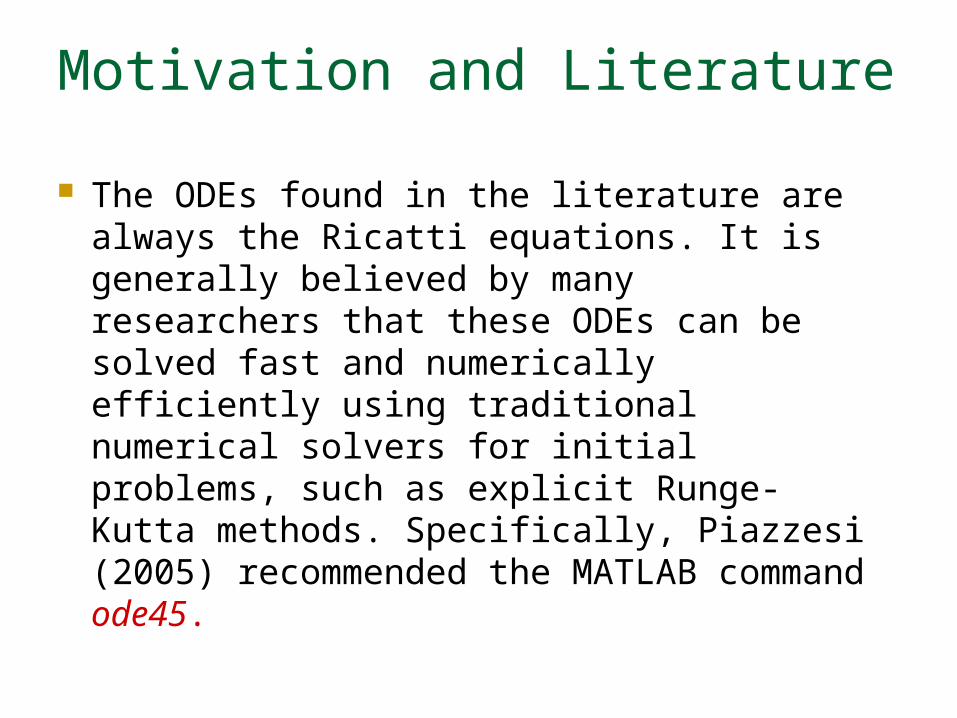
The ODEs found in the literature are always the Ricatti equations. It is generally believed by many researchers that these ODEs can be solved fast and numerically efficiently using traditional numerical solvers for initial problems, such as explicit Runge-Kutta methods. Specifically, Piazzesi (2005) recommended the MATLAB command ode45.


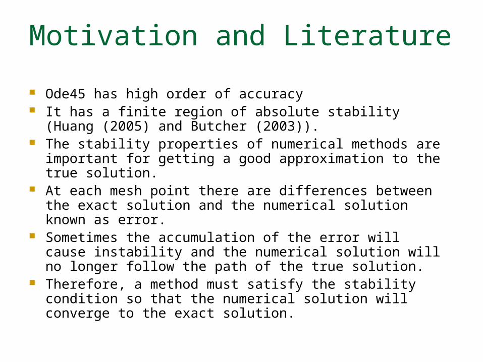
Ode45 has high order of accuracy It has a finite region of absolute stability (Huang (2005) and

Butcher (2003)). The stability properties of numerical methods are important

for getting a good approximation to the true solution. At each mesh point there are differences between the exact

solution and the numerical solution known as error. Sometimes the accumulation of the error will cause instability

and the numerical solution will no longer follow the path of the true solution.

Therefore, a method must satisfy the stability condition so that the numerical solution will converge to the exact solution.


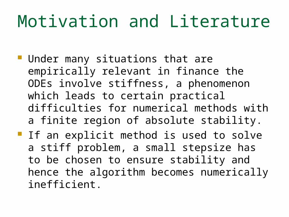
Under many situations that are empirically relevant in finance the ODEs involve stiffness, a phenomenon which leads to certain practical difficulties for numerical methods with a finite region of absolute stability.

If an explicit method is used to solve a stiff problem, a small stepsize has to be chosen to ensure stability and hence the algorithm becomes numerically inefficient.


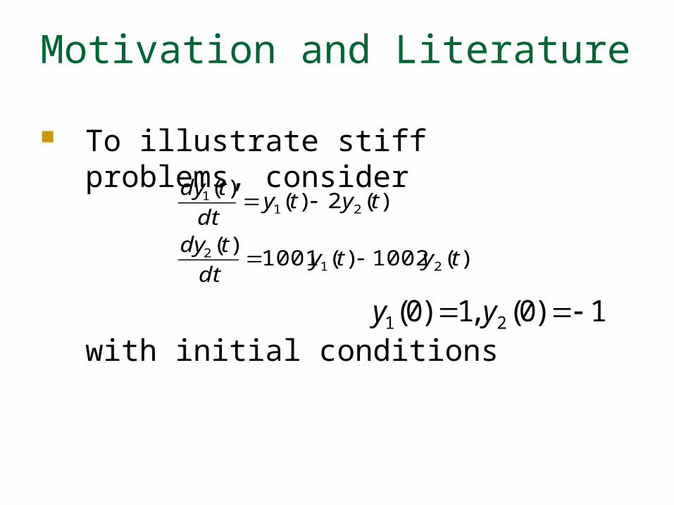
To illustrate stiff problems, consider

with initial conditions

)(1002)(1001)(

)(2)()(

212

211

tytydt

tdy

tytydt

tdy

1)0(,1)0( 21 yy


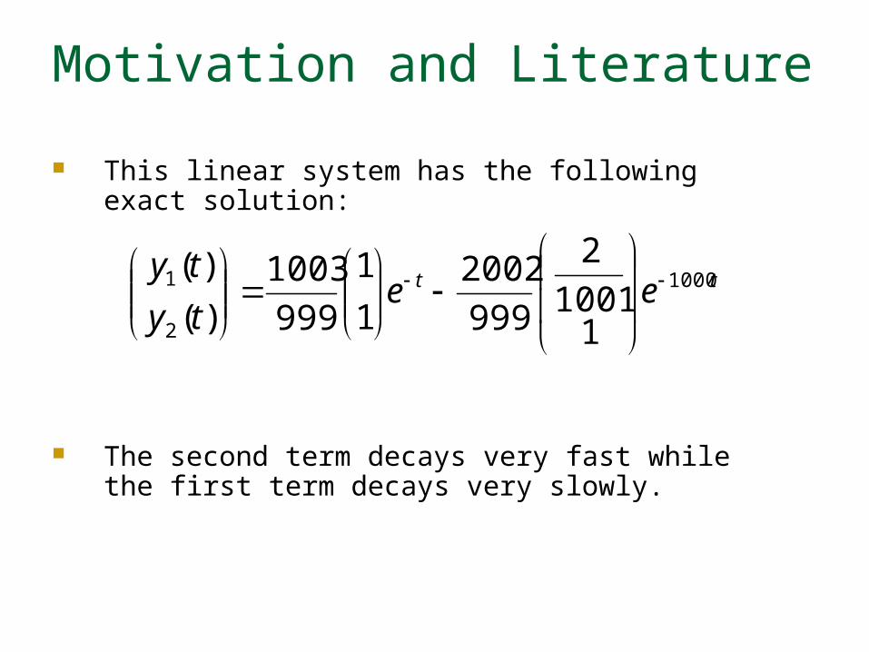
This linear system has the following exact solution:

The second term decays very fast while the first term decays very slowly.

tt eety

ty 1000

2

1

11001

2

999

2002

1

1

999

1003

)(

)(


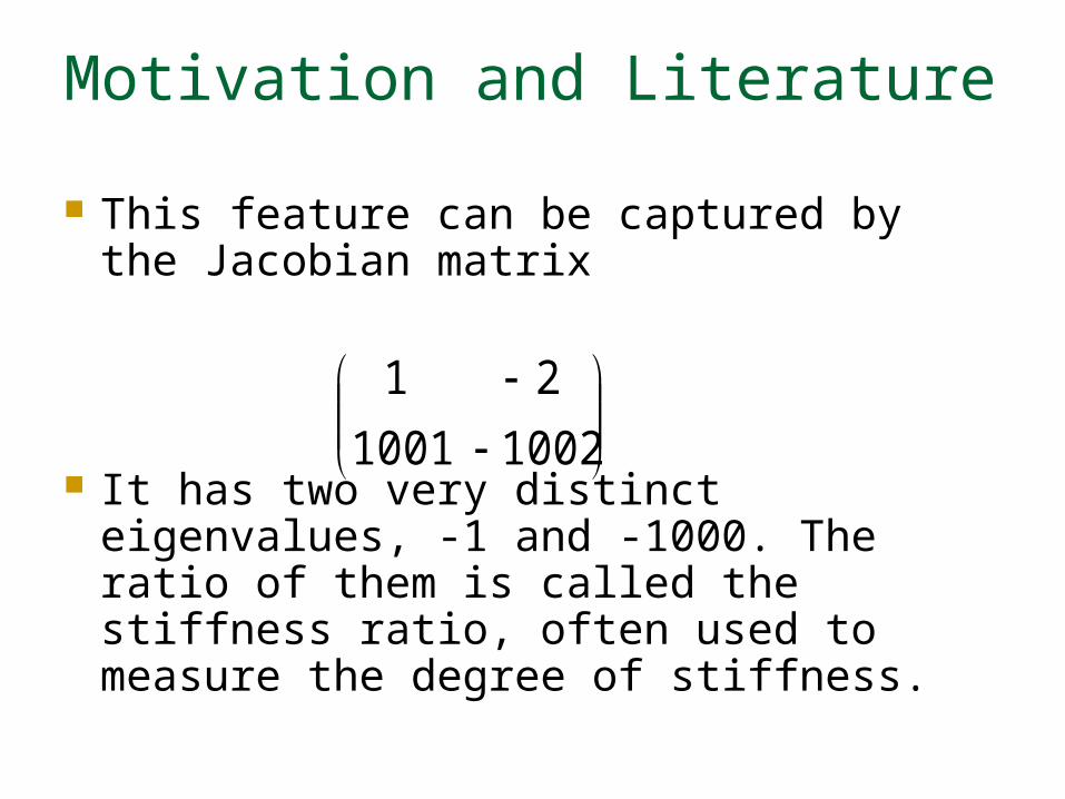
This feature can be captured by the Jacobian matrix

It has two very distinct eigenvalues, -1 and -1000. The ratio of them is called the stiffness ratio, often used to measure the degree of stiffness.

10021001

21


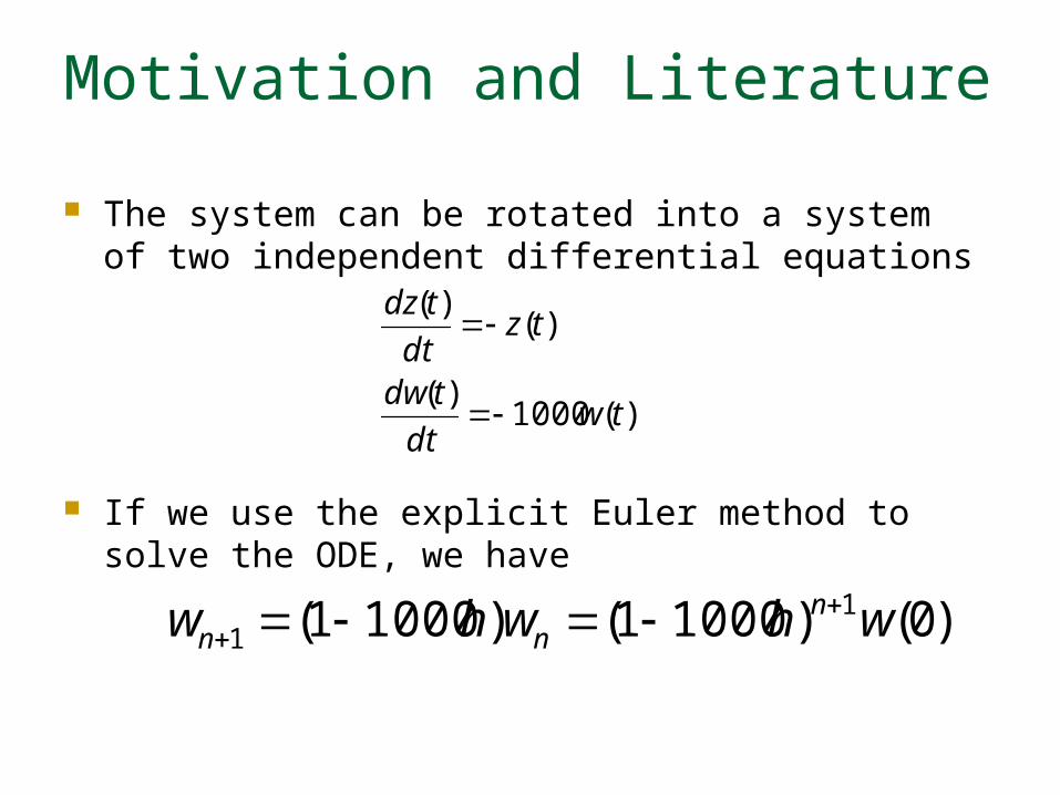
The system can be rotated into a system of two independent differential equations

If we use the explicit Euler method to solve the ODE, we have

)(1000)(

)()(

twdt

tdw

tzdt

tdz

)0()10001()10001( 11 whwhw n

nn


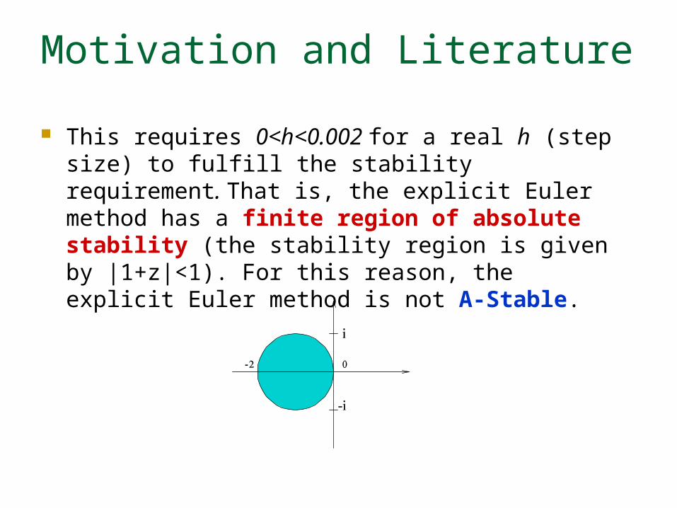
This requires 0<h<0.002 for a real h (step size) to fulfill the stability requirement. That is, the explicit Euler method has a finite region of absolute stability (the stability region is given by |1+z|<1). For this reason, the explicit Euler method is not A-Stable.


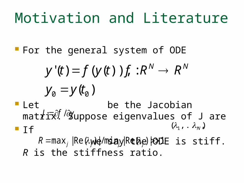
For the general system of ODE

Let be the Jacobian matrix. Suppose eigenvalues of J are

If we say the ODE is stiff. R is the stiffness ratio.

)(

:)),(()('

00 tyy

RRftyfty NN

yfJ /).,...,( 1 N

1|)Re(|min/|)Re(|max jjjjR


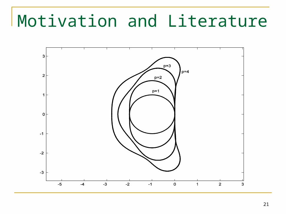
The explicit Euler method is of order 1. Higher order explicit methods, such as explicit Runge-Kutta methods, will not be helpful for stiff problems. The stability regions for explicit Runge-Kutta methods are as follows

21



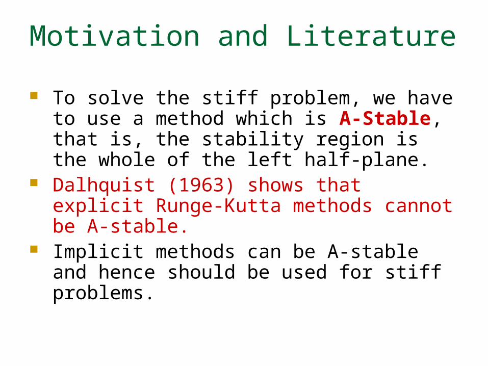
To solve the stiff problem, we have to use a method which is A-Stable, that is, the stability region is the whole of the left half-plane.

Dalhquist (1963) shows that explicit Runge-Kutta methods cannot be A-stable.

Implicit methods can be A-stable and hence should be used for stiff problems.


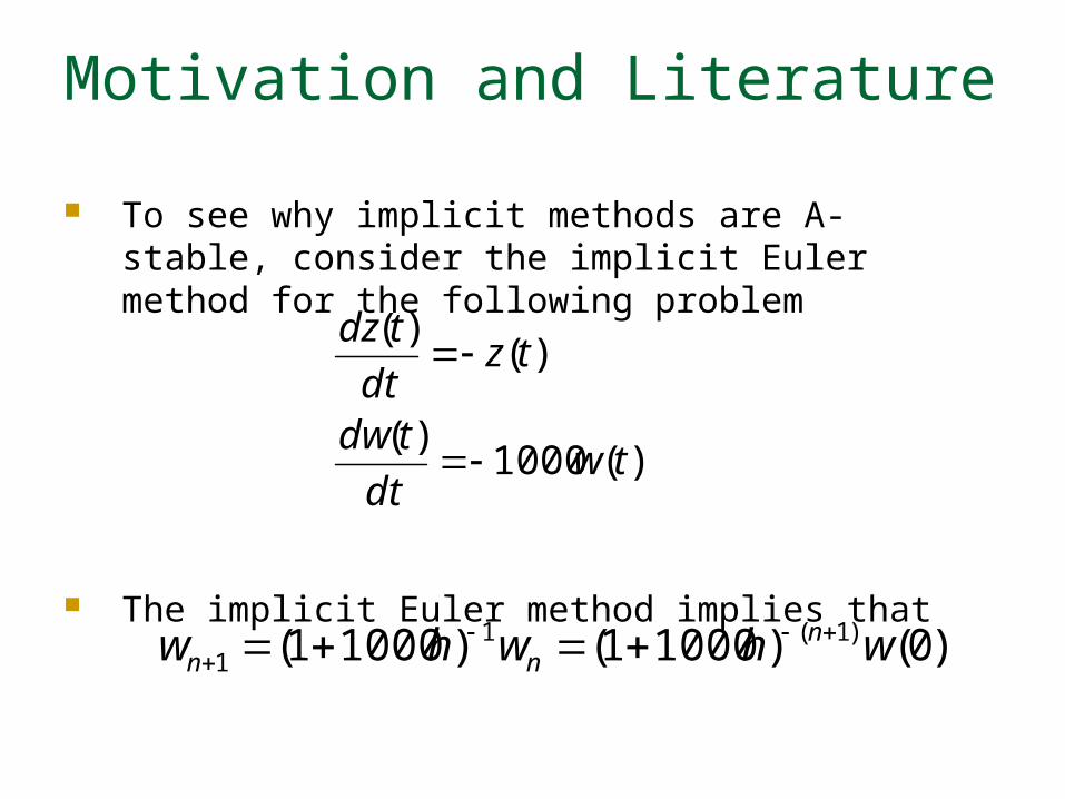
To see why implicit methods are A-stable, consider the implicit Euler method for the following problem

The implicit Euler method implies that

)(1000)(

)()(

twdt

tdw

tzdt

tdz

)0()10001()10001( )1(11 whwhw n

nn


So the stability region is


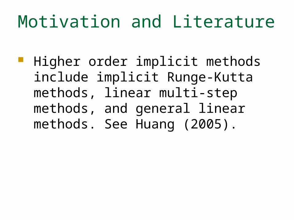
Higher order implicit methods include implicit Runge-Kutta methods, linear multi-step methods, and general linear methods. See Huang (2005).

Stiffness in Asset Pricing

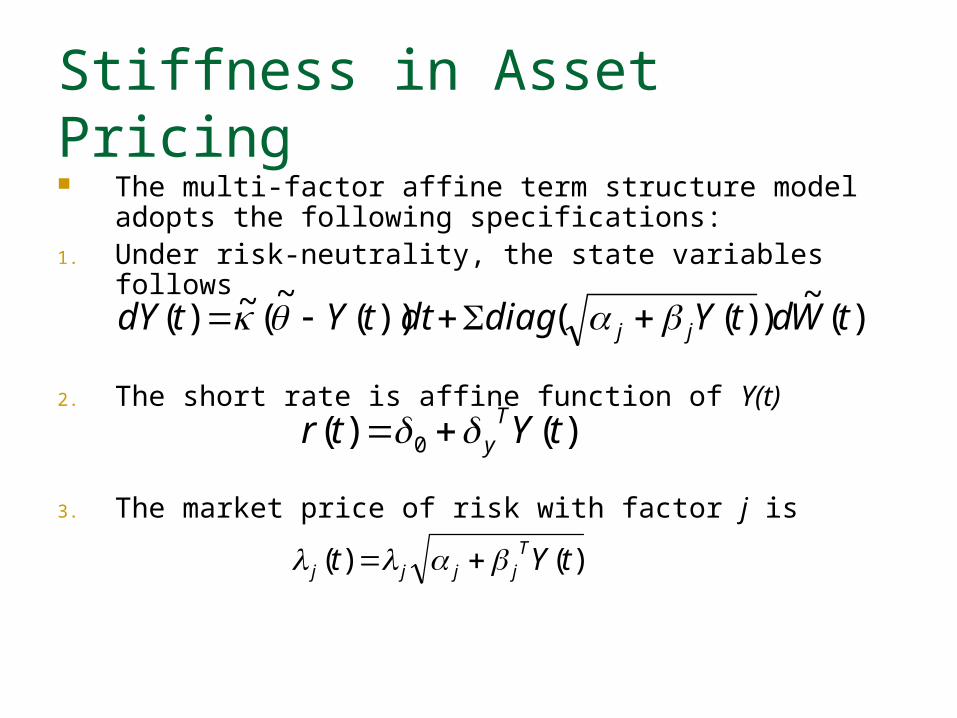
The multi-factor affine term structure model adopts the following specifications:

1. Under risk-neutrality, the state variables follows

2. The short rate is affine function of Y(t)

3. The market price of risk with factor j is

)(~

))(())(~(~)( tWdtYdiagdttYtdY jj

)()( 0 tYtr Ty

)()( tYt Tjjjj


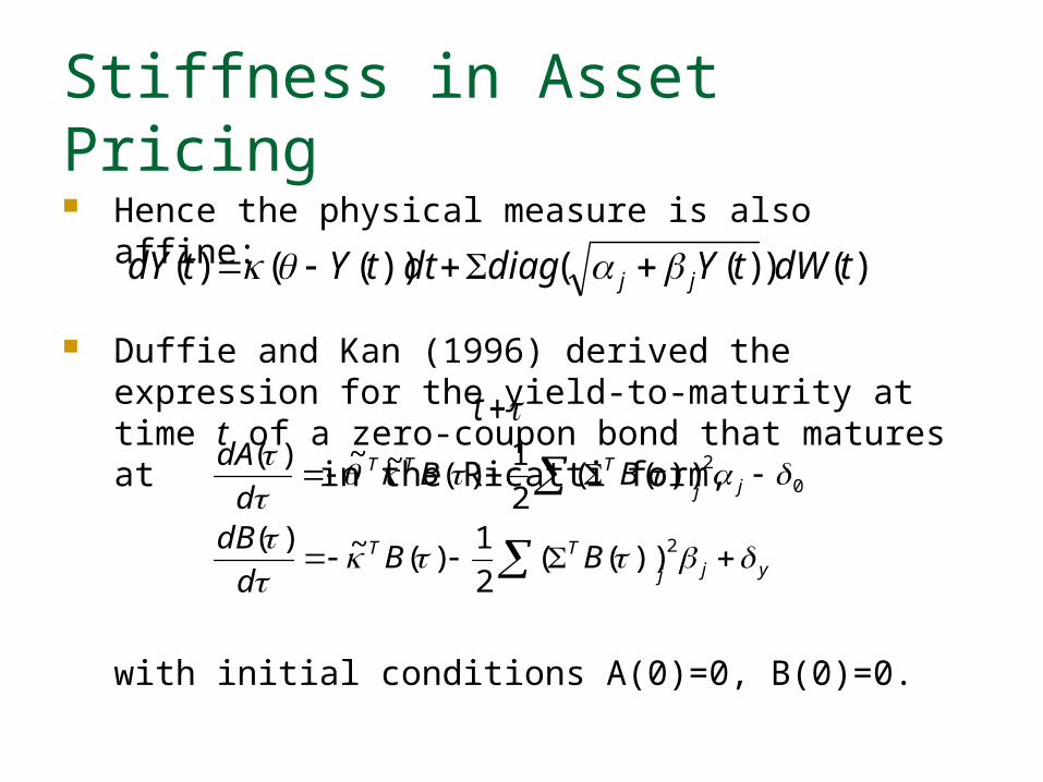
Hence the physical measure is also affine:

Duffie and Kan (1996) derived the expression for the yield-to-maturity at time t of a zero-coupon bond that matures at in the Ricatti form,

with initial conditions A(0)=0, B(0)=0.

)())(())(()( tdWtYdiagdttYtdY jj

t

yjj

TT

jj

TTT

BBd

dB

BBd

dA

2

02

))((2

1)(~)(

))((2

1)(~~)(


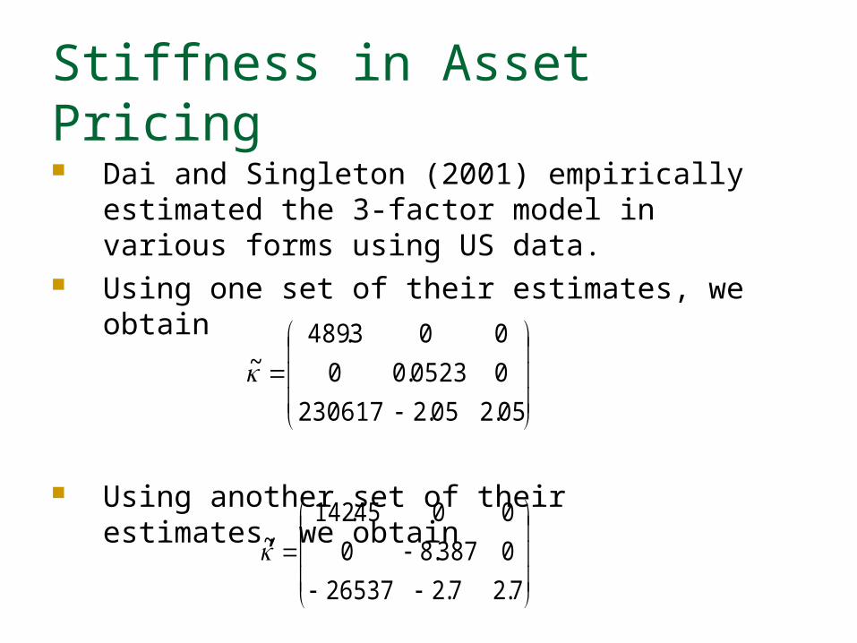
Dai and Singleton (2001) empirically estimated the 3-factor model in various forms using US data.

Using one set of their estimates, we obtain

Using another set of their estimates, we obtain

05.205.2230617

00523.00

003.489~

7.27.226537

0387.80

0045.142~


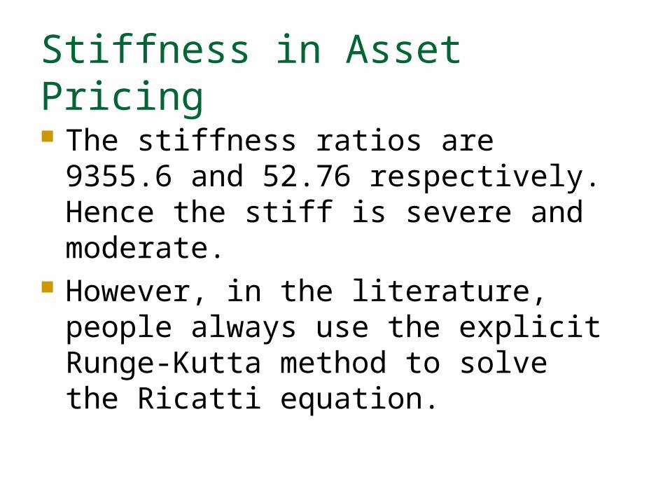
The stiffness ratios are 9355.6 and 52.76 respectively. Hence the stiff is severe and moderate.

However, in the literature, people always use the explicit Runge-Kutta method to solve the Ricatti equation.

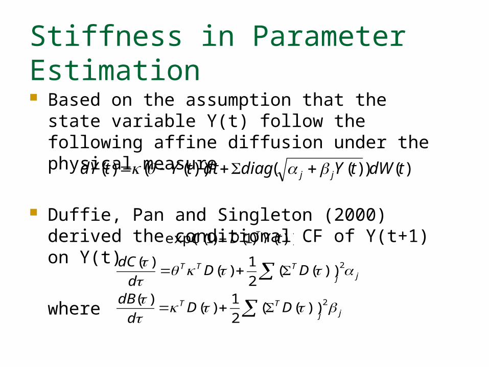
Stiffness in Parameter Estimation Based on the assumption that the state variable

Y(t) follow the following affine diffusion under the physical measure

Duffie, Pan and Singleton (2000) derived the conditional CF of Y(t+1) on Y(t)

where

)())(())(()( tdWtYdiagdttYtdY jj

))()1()1(exp( tYDC T

jj

TT

jj

TTT

DDd

dB

DDd

dC

2

2

))((2

1)(

)(

))((2

1)(

)(

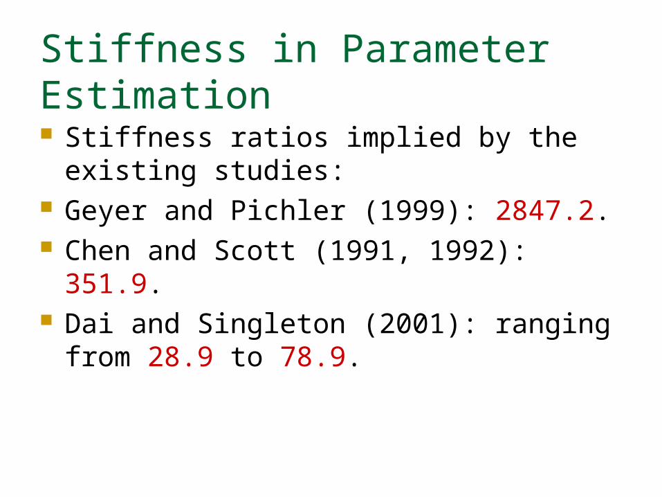
Stiffness in Parameter Estimation Stiffness ratios implied by the existing

studies: Geyer and Pichler (1999): 2847.2. Chen and Scott (1991, 1992): 351.9. Dai and Singleton (2001): ranging from 28.9

to 78.9.

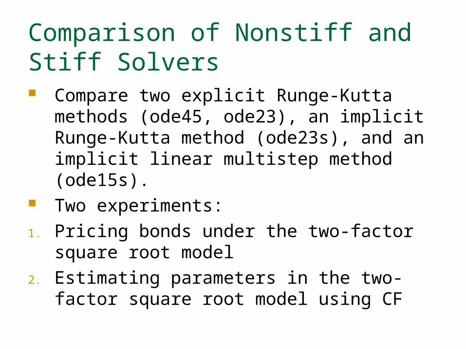
Comparison of Nonstiff and Stiff Solvers Compare two explicit Runge-Kutta methods

(ode45, ode23), an implicit Runge-Kutta method (ode23s), and an implicit linear multistep method (ode15s).

Two experiments:

1. Pricing bonds under the two-factor square root model

2. Estimating parameters in the two-factor square root model using CF

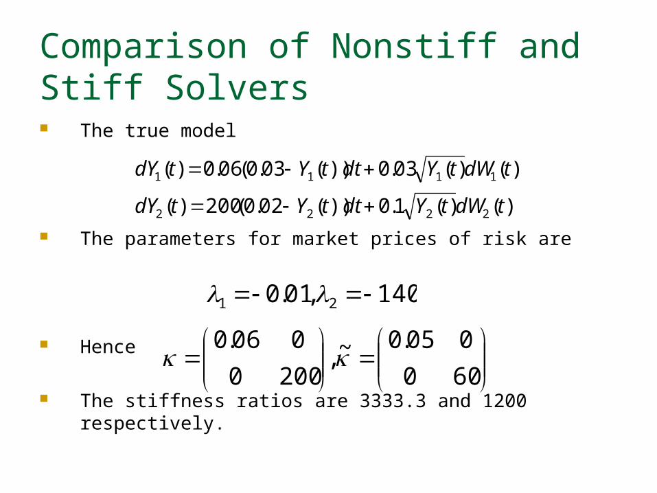
Comparison of Nonstiff and Stiff Solvers The true model

The parameters for market prices of risk are

Hence

The stiffness ratios are 3333.3 and 1200 respectively.

)()(1.0))(02.0(200)(

)()(03.0))(03.0(06.0)(

2222

1111

tdWtYdttYtdY

tdWtYdttYtdY

140,01.0 21

600

005.0~,2000

006.0

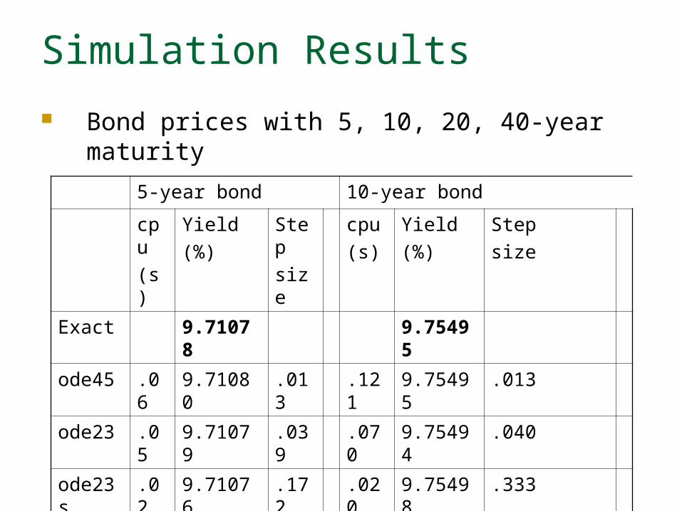
Simulation Results

Bond prices with 5, 10, 20, 40-year maturity

5-year bond 10-year bond

cpu

(s)

Yield

(%)

Step

size

cpu

(s)

Yield

(%)

Step

size

Exact 9.71078 9.75495

ode45 .06 9.71080 .013 .121 9.75495 .013

ode23 .05 9.71079 .039 .070 9.75494 .040

ode23s .02 9.71076 .172 .020 9.75498 .333

ode15s .02 9.71076 .089 .020 9.75490 .170

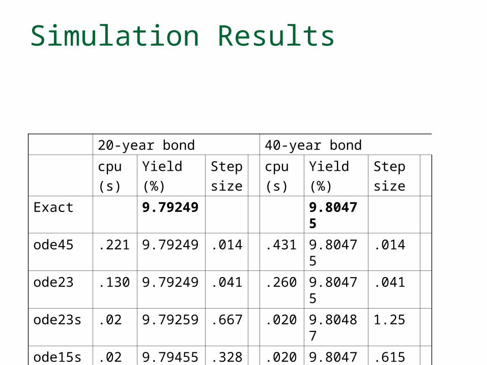
Simulation Results

20-year bond 40-year bond

cpu

(s)

Yield

(%)

Step

size

cpu

(s)

Yield

(%)

Step

size

Exact 9.79249 9.80475

ode45 .221 9.79249 .014 .431 9.80475 .014

ode23 .130 9.79249 .041 .260 9.80475 .041

ode23s .02 9.79259 .667 .020 9.80487 1.25

ode15s .02 9.79455 .328 .020 9.80475 .615

36

Simulation Results

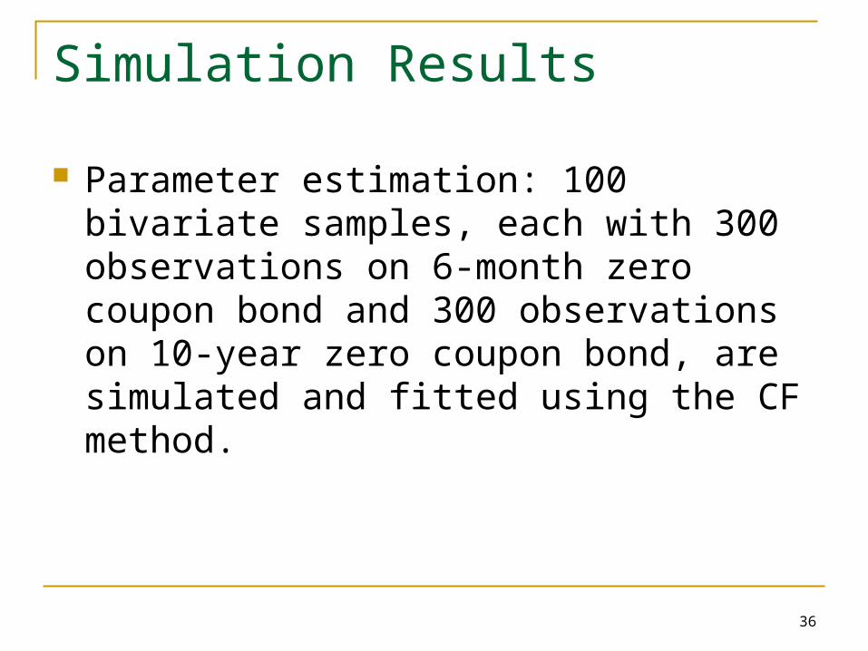
Parameter estimation: 100 bivariate samples, each with 300 observations on 6-month zero coupon bond and 300 observations on 10-year zero coupon bond, are simulated and fitted using the CF method.

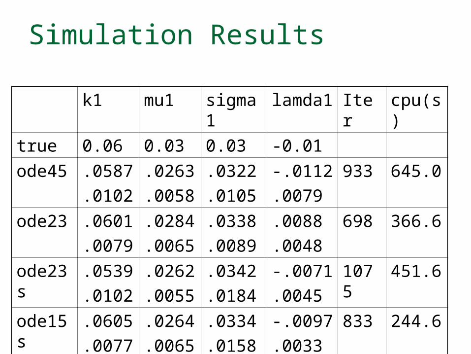
Simulation Results

k1 mu1 sigma1 lamda1 Iter cpu(s)

true 0.06 0.03 0.03 -0.01

ode45 .0587

.0102

.0263

.0058

.0322

.0105

-.0112

.0079

933 645.0

ode23 .0601

.0079

.0284

.0065

.0338

.0089

.0088

.0048

698 366.6

ode23s .0539

.0102

.0262

.0055

.0342

.0184

-.0071

.0045

1075 451.6

ode15s .0605

.0077

.0264

.0065

.0334

.0158

-.0097

.0033

833 244.6

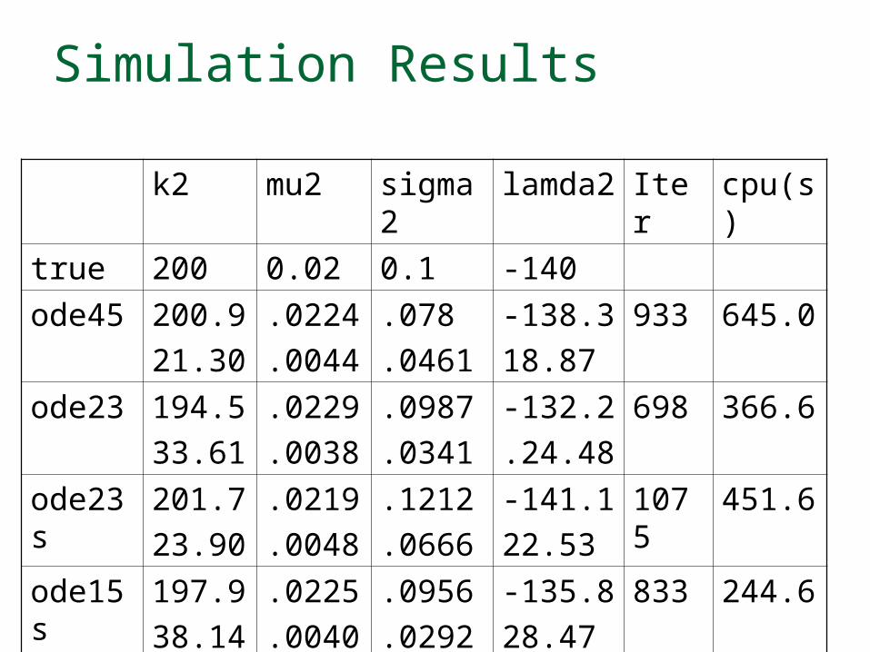
Simulation Results

k2 mu2 sigma2 lamda2 Iter cpu(s)

true 200 0.02 0.1 -140

ode45 200.9

21.30

.0224

.0044

.078

.0461

-138.3

18.87

933 645.0

ode23 194.5

33.61

.0229

.0038

.0987

.0341

-132.2

.24.48

698 366.6

ode23s 201.7

23.90

.0219

.0048

.1212

.0666

-141.1

22.53

1075 451.6

ode15s 197.9

38.14

.0225

.0040

.0956

.0292

-135.8

28.47

833 244.6

Conclusions

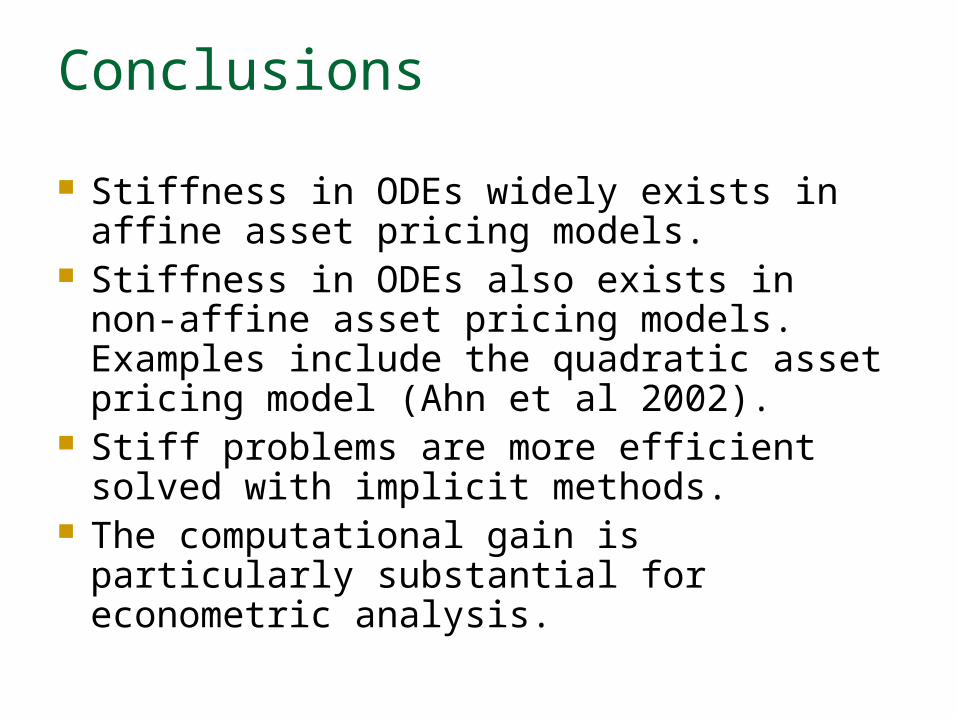
Stiffness in ODEs widely exists in affine asset pricing models.

Stiffness in ODEs also exists in non-affine asset pricing models. Examples include the quadratic asset pricing model (Ahn et al 2002).

Stiff problems are more efficient solved with implicit methods.

The computational gain is particularly substantial for econometric analysis.

Documents

On Stiffness in Affine Asset Pricing Models By Shirley J. Huang and Jun Yu University of Auckland & Singapore Management University