)

UNIVERSITY OF GOTEBORG DepartInent of Statistics

RESEARCH REPORT 1991:1

ISSN 0349-8034

ON SOME PREDICTION METHODS

FOR· CATEGORICAL DATA

by

Jonny Olofsson

Statistiska institutionen

GtlteIJorgs Univel'sitet Vi ktoriagatall 13 S 41125 Goteeorg Swedel}

ACKNOWLEDGEMENT

The author is grateful to Associate Professor Marianne Frisen,

who suggested the topic for the paper and provided considerable

encouragement and valuable comments during the course of the

work.

He also wishes to thank Mr Christer Andersson for carefully

reading the manuscript and Mr Staffan Geissler who printed the

manuscript.

ABSTRACT

Good prediction methods are important in many fields where

qualitative variables are involved. The criterion of a good

prediction method, used in this paper, is the average mean

squared error. This criterion is used to compare and derive

prediction methods, when the variable of interest is binary.

The methods considered here are based on the maximum­

likelihood estimators of the expectation of the binary varible,

for which we want to make a prediction. Derivations and

simulations are made for the case where we have one qualitative

background variable. It is for example demonstrated that, when

the ordinary chi-squared test is used for choosing between two

prediction methods, it should not be adopted on a conventional

low level of significance (e.g. 5%).

CONTENTS

1 Introduction 1

2 Different kinds of predictions and measures of

prediction error 5

2.1 Event predictions and actuarial predictions 5

2.2 Measures of prediction error 7

2.3 Model selection procedures 14

3 Models and notations 18

4 Derivation and comparisons of prediction rules 25

4.1 The average mean squared error for the

predictors based on the unrestricted

and the restricted model

4.2 The suggested predictor Pb-.

4.3 Comparison of Pb- and predictors based on

Pearson's chi-squared test

4.4 Comparison of Pb- and predictors based on

the Akaike-criterion

25

32

35

41

4.5 Effects of different sampling proportions

in the old and the new sample

4.6 The multinomial case

4.7 Figures

5 Concluding remarks

Appendix

References

44

49

52

65

66

1. INTRODUCTION

In this paper we consider model selection, when faced with a

binary dependent variable, Y, and a number of qualitative

background variables. In an application Y could, for example,

correspond to the presence or absence of a certain disease, and

the background variables could be, e.g. exposed/not exposed,

sex, living area. The data can be organized in a mUlti­

dimensional contingency table, where each cell contains the

number of observations for a certain combination of variable

values.

1

Even for a moderate number of background variables, there are a

large number of cells in the table, and therefore there is

often a wish to reduce, if possible, the dimensionality of the

table. Traditionally this reduction has been accomplished by

fitting various log-linear models to the data and removing

parameters from the model that have proved non-significant

according to some kind of statistical test, thus obtaining a

non-saturated model, i.e. a model containing fewer parameters

than cells in the table. Section 2.3 gives a brief discussion

on such procedures. By estimating the parameters of a

particular model, we can also obtain estimates of the

conditional probability of Y given the values of the background

variables.

It is not self-evident that the traditional strategy, involving

testing of hypotheses, is the best for all purposes. The

purpose of the analysis can, for example, be to obtain

information about the causal structure or to obtain predictors

that will minimize some measure of error. We will in this paper

concentrate on the latter aim, restricting the analysis to

the class of predictors, where the maximum-likelihood (ML)

estimates replace the parameters of a 'good' model. The problem

is thus to find 'good' models for prediction purposes. This

approach has similarities with the traditional ones and might,

besides giving good predictors, also give some insight in to

the structure of the data. The principal theoretical

differences between the statistics suitable for traditional

testing of hypotheses and those suitable for prediction

purposes, are also of interest.

2

The problem of choosing models for prediction purposes has been

extensively studied in the area of multiple regression

analysis. A criterion for model selection frequently adopted is

the mean squared error of prediction (MSEP). For observation

of a future value of a binary dependent variable Y, MSEP is

defined as E(y-p')2, where p' is a predictor of Y. As the

MSEP takes account of both bias and sampling variability, we

have the result that the saturated model is not necessarily the

best. A bias can very well be offset by a reduced sampling

variability owing to the inclusion of fewer estimated

parameters. The MSEP depends on parameters which usually have

to be estimated.

It must be noted here, that we do not argue that the selected

model is the "true" one. That is, in selecting a non-saturated

model, we have not proved that the remaining effects are equal

to zero. All we can say is that the selected model has the best

prediction ability as judged by the criterion used in the

study (with the reservation that the criterion is estimated on

the basis of data).

Chapter 2 presents a brief discussion on two different kinds of

prediction methods for binary data. Different measures of

prediction error are also considered. The chapter ends with a

short review of some procedures for selection of models.

3

Chapter 3 introduces notations and a measure of prediction

error, for the case where we want to make predictions about a

binary variable and where we have observations on a discrete

background variable, Z. When making a prediction for a

particular level of Z, we distinguish between two predictors.

The first is the usual maximum-likelihood estimator of the

probability of success and the second is the maximum-likelihood

estimator, which is obtained under the restriction that all

success probabilities are equal (i.e. homogenity). In the

following these predictors will be referred to as the

unrestricted and restricted predictor, respectively.

In Chapter 4, we examine a measure of prediction error, the

average mean squared error, AMSE, for both prediction rules. A

criterion based on AMSE for choosing between the two prediction

rules is developed. The AMSE for this combined prediction rule

is compared with the AMSE for the rules pI and p*. We also

study the AMSE of the prediction rule that is obtained by

letting a chi-squared test of homogeneity make the selection

between pI and p*. The AMSE-criterion is also compared with

the so called Akaike-criterion.

4

2. DIFFERENT KINDS OF PREDICTIONS AND MEASURES

OF PREDICTION ERROR

2.1 Event predictions and actuarial predictions.

When making predictions of a variable, we often use known

values of other variables, in some way related to the unknown

variable. The variable for which we want a prediction is called

the dependent variable, while the other (background-) variables

are termed independent. In this section we discuss some

distinctions among alternative kinds of predictions, when both

the dependent and the independent variables are categorical. As

the prediction ability of a specific model can be used as a

criteria for model selection, we will also look at some

measures of prediction error.

5

Hildebrand et al. (1977) make a distinction between an event

prediction and an actuarial prediction. An event prediction is

a proposition that predicts each case's state on the dependent

variable, while an actuarial prediction is a proposition which

specifies, for each case, the probabilities of the dependent

variable. As an example of an event prediction rule the authors

take the case of a binary dependent variable and two

independent variables:

"If the legislator is liberal from an urban district

then predict that that person will vote in favour

of the bill"

An example of an actuarial prediction is:

6

"The chance of rain during each day in July is 1/3"

In the first case an investigator could determine, for any

"liberal from an urban district", whether the prediction was

correct once the vote has been cast. In the second case the

investigator could evaluate the extent to which the observed

proportion matched the predicted. Usually, both kinds of

predictions are based on past data. Having noted a proportion

of 1/3 rainy days in July over a number of years, we could make

the prediction "no rain" for a certain day in July, because

this alternative is the most likely.

In many cases it seems reasonable to associate an actuarial

prediction with an individual future observation. Instead, for

example, making an event prediction and classifying a patient

as either healthy or sick, we come up with a proportion

reflecting the risk of having the disease. Increasing values of

the prediction could perhaps correspond to actions reaching

from surveillance, via drug treatment, up to surgical

treatment.

2.2 Measures of prediction error.

The topic covered in this paper, is a special case of a more

general problem where one wants to choose a model suitable for

prediction purposes. See Linhart and Zucchini (1986) for

examples of application in different fields. In the literature

the measure of prediction error is often termed error rate and

one distinguishes the optimum error rate, which is the error

rate that can be obtained if the parameters of the statistical

model are known and the optimal predictor is used. Secondly,

the actual error rate, is the error rate obtained by averaging

over the the distribution of future observations. Thirdly, the

apparent error rate is defined to be the average error rate

when the predictor is applied to the available observations

retrospectively. A trivial example should illuminate these

concepts.

7

Suppose we observe a sequence of independent random variables

Y1, ••. ,Yn , with common mean ~ and variance 0 2 . Suppose that we

want to use these observations to make a prediction of a future

observation Ynew , thought to have the same distribution. Now,

suppose we adopt the mean squared error to a particular

predictor Y', for example the mean of the observations Y1, •• Yn .

The actual error rate then becomes

MSEact = E(Ynew - y,)2

If the parameter p were known, we could use it as a predictor

and we would obtain the optimum error rate

MSEopt= 0 2

For the apparent error rate we let the predictor Y' predict the

observations retrospectively and average the squared errors

MSEapp

Much research has been devoted to estimating the expectation of

actual error rate (the apparent error rate is generally biased

downward). Van Houwlingen and Le Cessie (1989) gives a review

of different ways for estimation, including cross-validation.

Efron (1986) provides several estimates for the bias of the

apparent error rate. The theory applies to general exponential

family linear models and general measures of prediction error.

8

In a setting identical to the one in this paper, where there

are several groups of observations on a binary variable, Efron

(1978), constructs one-way ANOVA tables, by introducing a wide

class of measures of binary variation, including the squared

error. A coefficient of determination can thus be defined for

each measure in the class, reflecting the proportional decrease

in residual variation when going from a crude explanation of

the probabilities of success in the groups, to a more detailed.

9

In the case of event predictions, we are either right or wrong,

so one appropriate measure of prediction error is the apparent

error rate:

The number of false predictions divided

by the total number of predictions

Consider the following example, where we have some past data of

how urban legislators voted in a similar election.

Liberal Conservative

In favour 10 50

Against 30 10

Suppose we adopt the strategy of predicting "against" for

liberals and "in favour" for conservatives. The apparent error

rate in this case equals 0.20 and can be interpreted as

follows. Suppose we knew only the state of the independent

variable for all 100 individuals and used the proposed strategy

to predict the state of the dependent variable of a randomly

selected individual. The probability of making a false

prediction would then be 0.20. This rate could be used for

comparing other prediction rules, e.g. predicting "in favour"

for both liberals and conservatives.

Since the apparent error rate was obtained by letting the

sample predict itself, we might suspect that it is to

optimistic for future data. That this is the case is shown in

Efron (1986).

Turning to actuarial predictions where the predictor is

continuous on the interval (0,1), we are more flexible when

choosing a measure of prediction error. In the setting of the

two-way classification of above, we define the squared

prediction error for a future observation, i, belonging to

state j on the independent variable

where Pj' is an estimate of the probability p(Y=llz=j). The

actual error rate in this case is

When the aim is to compare the performance of different

predictors, we could of course drop the constant term

10

Pj·(l-Pj). In chapter 4, we will study the expectation of a

weighted average of this error rate over the values of j for

two different predictors.

Another measure is the expectation of the Kullback-Leibler

distance. For a single Bernoulli variable Y with expectation p

this is defined as:

Dact E( -Y·log(p') - (l-Y)·log(l-p') )

-p·log(p') - (l-p)·log(l-p')

11

where p' is a predictor of Y and the expectation is taken over

Y, holding p' constant. It is equal to the expectation of the

log-likelihood over Y, holding p' constant. We see that for Y=l

the Kullback-Leibler distance is equal to -log(p'), a

decreasing function of p' and for y=Q it is equal to

-log(l-p'), an increasing function of p'. The apparent error is

Dapp -p'·log(p') - (l-p')·log(l-p')

If we in the two-way classification assume that we observe one

binomial variable Xj for each level of the independent

variable, with parameters (nj,Pj) j=1,2, •. ,k, the Kullback­

Leibler discrepancy can be written as

Dact

where Pj' j=1,2, are predictors of Yijo The apparent error

becomes

Dapp = - E Pj'olog(Pj') - E (nj-Pj')olog(l-Pj')

Now, the difference Dact - Dapp can be written as

Approximating log(Pj/(l-Pj'» with the first two terms in it's

Taylor expansion, the expectation of Dact - Dapp is

If we for example let Pj' be the ordinary ML-estimator of Pj,

this expectation is equal to 2/no If we have k different

binomial populations the expectation would be kino Adjusting

Dapp with the bias approximation we get

D- = Dapp + 2/n

12

This in turn is equal to

- I + 2/n

where I is the maximized log-likelihood.

In fact, this is a special case of the generalized information

criterion for model selection, which states that one should

choose the model for which

is maximum. Ii is here the log-likelihood for the i:th model,

maximized over qi parameters. In our case a is equal to 2 and

this corresponds to the Akaike information criterion. For a

discussion of this and the generalized information criterion

see Atkinson (1980) and section 4.4.

13

2.3 Model selection procedures.

When we have decided on a particular measure to compare models,

there are different ways to search for the "best" model. For

multidimensional contingency tables, one often considers the

class of log-linear models, where it is assumed that the

logarithms of the cell probabilities depend additively on a

number of so called effects. For a three-dimensional table a

log-linear model can be written

where Pijk i=O,l j=1,2 ••. ,J k=1,2 ••• ,K

14

This is the saturated model, e.i. it contains as many effects

as there are cells in the table. Unsaturated models are

obtained by removing effects. It is a common practice to

restrict attention to a family of submodels, called

hierarchical models. The hierarhical principle means that if an

effect is set equal to zero, then all its higher-order

relatives are also set equal to zero. In the three-dimensional

case, if for example the second-order interaction (a~)ij is

zero, the hierarchical principle means that the third-order

interaction (a~o)ijk is also zero. As we are more interested in

modelling Pjk, the probability of Y=l given the values of the

independent variables, we note that the 10git of this

probability can be expressed as the difference between two 10g­

linear models

As the number of possible models increases rapidly with the

number of variables in the table, many model selection

procedures have been developed. These procedures end up with

one or several models hoped to be adequate in some way.

15

Most strategies for model selection begins by the fitting of a

starting model. Adopting a rule for stepping from one model to

another, one searches over a subset of the possible models. The

process stops when some termination criterion is fulfilled.

In most selection procedures the stepping rule and the

termination procedure, depend on a goodness-of-fit test. Two

commonly used test statistics are the Pearson chi-squared

statistic and the log-likelihood ratio statistic.

The selection procedures can be divided into three types, which

all have a counterpart in multiple regression analysis.

Starting from a simple model (often consisting of the main

effects only), one conducts forward stepping by successively

including effects. In backward stepping one starts with a

complex model (often the saturated model), and successively

removes effects. Greater flexibility is obtained if we allow

effects previously added to the model to be removed in a later

state or allow an effect removed in an earlier state to be

included again. Virtually all procedures end when the tests

employed for the addition of a term are nonsignificant or the

tests for the removal of a term are significant. Benedetti and

Brown (1978) summarize several of these procedures and

illustrates their performance by an example.

If the aim is to make hypothesis tests of effects, there is a

problem of controlling the overall significance level. Aitkin

(1979) has developed a simultaneous test procedure for fitting

models, which is based on a backward stepping procedure.

Fowles, Freeney and Landwehr (1988) construct a scatterplot

for the d.f. (degrees of freedom) versus the value of the log­

likelihood statistic for all possible models. Points that fall

near the line (d.f.,d.f.), fit the data well since the

expectation of the test statistic equals the number of degrees

of freedom if the model is correct and the samplesize is large.

Points to the right of the plot (large d.f.) represent simple

16

models. Suggestions are made to select a subset of models with

high d.f.:s near the line (d.f.,d.f.) for further inspection.

This is an analogy to the Mallow's Cp-plot for multiple

regression.

17

3. MODELS AND NOTATIONS.

From now on we will be concerned with some simple special

cases of choosing a model for a cross-classification when the

objective is to make predictions of a binary variable, Y. We

assume that we have observations on Y and an attribute Z, which

is purely nominal. The data can be presented in a contingency

table

Z

I 2 3 •••••••••••••••••••••• k

0 xOI x02 x03· ................... xOk xO.

Y

I x11 x12 x13-····.············· .xlk xl.

x .1 x .2 x.3-.··· .. ··· .. ·· ... ·· .x.k x m

=m1 =m2 =m3· ................•.. =mk

where Xij is the number of observations in cell (i,j), and

summation over an index is indicated by a dot. The aim is to

use these data when making predictions for future values of Y.

18

19

The corresponding notations for the probabilities will be

Z

1 2 3 ••••••••••••••••••••• k

0 POl P02 P03· .................. POk PO.

Y

1 P11 P12 P13· .................. Plk Pl.

P.1 P.2 p.3-················· ·P.k P •• = 1

Defining

P1j

Pj E( y I Z=j ) j = 1,2, ••• ,k

POj+P1j

we want to obtain an estimate of each Pj and use it as a

predictor of future observations on the binary variable Y. Thus

we are dealing with actuarial prediction. This is also the

simplest example of variable selection, where we have only one

independent variable.

For the two-way classification above we can formulate a

saturated log-linear model as

where lij=log(Pij) and ~ai=~~j=~~(a~)ij=O. For situations where

one variable can be interpreted as response and the other as

explanatory, log-linear models that condition on the margins

of the explanatory variable, that is, logistic regression

models are of interest.

p' + ~j'

20

We assume that the Xlj:s are distributed as independent

binomial variates, which is equivalent to assuming that the

marginals x.j:s are fixed. In section 4.6 we will look at the

case where only the total sample size is fixed, e.i. the Xij:s

are multinomially distributed. The relation ~l'= ~2'= ••• =~k'= 0

corresponds to equality of the probabilities Pj, e.i.

homogenity. Thus we have two possible logistic models, one

including only the constant term p', the other also including

the effect ~j'.

Restricted model: log(Pj/(l-pj» p'

Unrestricted model:

A selection procedure in this case, thus amounts to choosing

between these two model. A common approach is to adopt some

test of the hypothesis HO: ~j'=O and choose the larger model if

this test is rejected. As this paper deals with prediction of a

binary variable, we want to obtain estimates of Pj:s under both

models. Generally, to derive M.L.-estimates of the effects in a

logistic model, we need iterative methods. Replacing p' and ~j'

with their estimated values, we can get the M.L.-estimates for

the Pj:s. For the restricted model we obtain a single

estimate for all Pj:s, while for the unrestricted model they

generally differ. In this case, where we have just one

independent variable and thus no interaction effects, we can

compute the M.L.- estimates directly, without fitting a

logistic model.

Now, assuming the restricted model is correct (e.i.

homogenity), the M.L.-estimator of the Pj:s is the sum of the

number of successes for each level of Z, divided by the total

number of observations. We make the notation

If the unrestricted model is correct, we obtain the M.L.­

estimators

21

i.e. the number of successes divided by the number of

observations for Z=j. p* and Pj' will be referred to as the

unrestricted and restricted estimator/predictor, respectively.

In the following we let Pj' and p* denote both the stochastic

variable and a particular realization.

As a measure of prediction error, we will adopt squared error,

that is

and

where Yij is a new observation independent of the Xij:S but

identically distributed. Following the terminology of chapter

2, the actual error rates are obtained by taking expectation

over Yij, holding Pj' and p* constant.

Comparing the performance of the two predictors, we drop the

common term Pj·(l-Pj) and take expectation also over Pj' and

* Pj respectively. We make the notation

and

22

23

where MSE stands for 'mean squared error'. Of course, both

MSE:s depend on unknown parameters and have to be estimated.

Now, if we make a new observation for which Z=j, we would

prefer the predictor Pj' if

Turning to the case where we want to predict a whole sample of

new observations, with sampling proportions f1, f2, •• ,fk, we

assume that the aim is to select a vector of predictors that

is on the average good for the whole new sample. We will

consider two such vectors, namely

P' = (P1', P2 ' , ...• , Pk ' )

p* ( * * *) P1 , P2 , •••• , Pk

both of dimension k. Thus for the prediction rule P'; if Z=j

for an observation, use Pj' for prediction. And for the rule

p*; if Z=j use p* for prediction. We define the average mean

squared error for the two prediction rules as

AMSE( PI)

AMSE(P*) * = 1: fj·MSE(Pj )

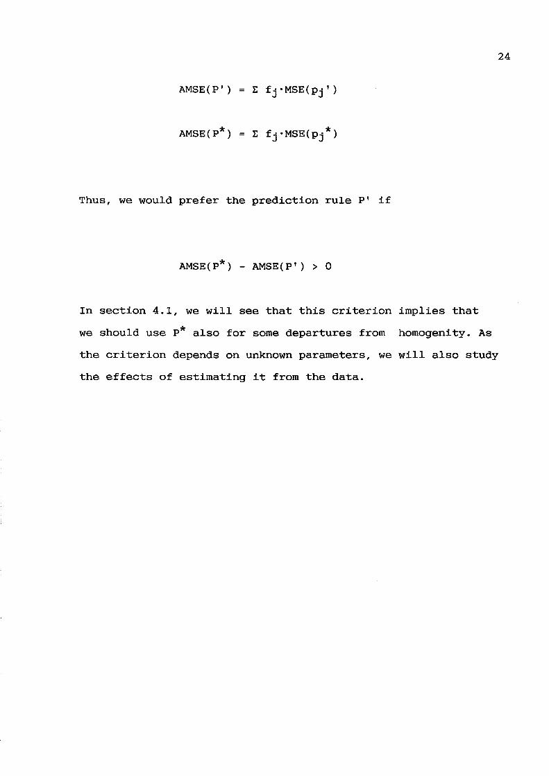
Thus, we would prefer the prediction rule pI if

AMSE(P*) - AMSE(P I ) > 0

In section 4.1, we will see that this criterion implies that

we should use p* also for some departures from homogenity. As

24

the criterion depends on unknown parameters, we will also study

the effects of estimating it from the data.

25

4. Derivation and comparisons of prediction rules.

4.1 The average mean squared errors for the predictors based on

the unrestricted and the restricted model.

In this section we study the average mean square error criteria

for choosing between the two predictors p'and p*. We should use

the predictor P' for a sample of new observations if

AMSE(P') - AMSE(P*)

is larger than zero and otherwise using the predictor p*. Of

course, this criterion depends on unknown parameters, which in

practice have to be estimated. Before we turn to this, we will

examine how the AMSE:s depend on the true parameters. We will

also study the shape of the region in the parameter space where

P'is preferred to p*.

Now, recall that we have available observations Xlj with

corresponding sample sizes mj , j=l,2, •.. ,k. We want to use the

old data set to make a prediction rule for new observations

from a population with the same probabilities Pj, but with

possibly different sampling proportions. The risk of the

unrestricted predictor p' can be written as

26

AMSE(P' )

Until section 4.5 we assume that the sampling proportions in

new sample are equal to the sampling proportions in the old

sample, i.e. fj=mj/m for j=1,2, ... ,k. AMSE(P') can then be

written as:

AMSE( P' ) I: Pj· (1-Pj )/m

For k=2 we can rewrite this as:

AMSE(P' )

so

The surface is thus a cap of an elliptical parabola with vertex

in the point (0.5,0.5, 112m). The height of this cap depends

inversely on the total sample size.

27

For the predictor p*, we get

AMSE(P*)

* where n = E(p ) = t fj·Pj

Thus, AMSE(P*) consists of two parts, measuring the variance

and the bias respectively. We note that the variance part is

always less or equal than AMSE(P'). For k=2, AMSE(P*) is equal

to

AMSE(P*)

(4.1.1)

In fig 4.1.1 and 4.1.2 we plot AMSE(P*), for different values

of PI and P2=1-Pl and P2=0.5-Pl respectively. The total

samplesize, m, is set equal to 30 in these and the following

figures. We have also plotted AMSE(P'). These lines as well as

the line P2=0.1-Pl are shown in fig 4.1.3.

The intersection of the graphs of AMSE(P*) and AMSE(P') defines

the interval where performs p* better than P'. Due to a

reduced bias term, this interval increases when fl moves away

from 0.5. The length of the interval depends inversely on the

total sample size.

Write the criterion AMSE(P*) - AMSE(P') > 0 in the form

> 1

28

where the index b refers to the binomial case. By making an

appropriate change of coordinate system we will show that for

k=2 relations of the kind ob=d defines an ellipse in the

PlxP2-space. Put

PI x·cose - y·sine

P2 = x·sine + y·cose

Substituting this into ob=d, we get

A·x2 + B·x·y + C·y2 + D·x + E·y o (4.1.2)

where

A (l+d/m1)·COS2a - 2·cosa"sina + (l+d/m2)·sin2 a

B -(d/m1 - d/m2)"sin2a - 2·cos2a

C = (l+d/m1)·sin2a + 2"cosa·sina + (l+d/m2)·cos2 a

D -(d/m1)·cosa - (d/m2)·sina

E (d/m1)·sina - (d/m2)·cosa

Putting B=O is equivalent to

cot2a

Solving for a

29

(4.1.3)

It is easily seen that, since d>O, both A and B are larger than

zero for all values of a. This proves that the relation 0b=d

defines an ellipse. For f1 = 0.5, a = n/4. Substituting this

value into (4.1.2), we arrive at

o

Completing squares and rewriting in the standard formula for an

ellipse we get

------------ + --------------- = 1 (4.1.4)

1/2 d/2· (m+d)

30

The area inside the ellipse for d=1, defines together with the

requirement O~P1,P2~1, the region where p* is preferred to p'.

The eccentricity of this ellipse is

1

(m + 1)2

31

and thus it becomes flatter for large m, and because the major

axis is constant this indicates that the region where p* is

preferred becomes smaller. By looking at (4.1.3) and ( 4.1.4) ,

we see that the major axis coincide with the P1 =P2-line if

f1=0.5. For f1+0.5, the major axis is tilted off this line.

The magnitude of this effect is inversely related to m. For a

total sample size of m=30, the region was plotted for two

cases, f1=15/30 and f1=5/30. The result is shown in fig 4.1.3,

where it is seen that the region is larger for f1 = 5/30. By

inspecting (4.1.1), we see that this is no accident, since as a

function of f 1, AMSE ( p* ) reaches its maximum for f 1 =0. 5 and

AMSE(P') don't depend on fl.

4.2 The suggested predictor Ph-.

Now, ideally we would use the predictor P 'whenever ob> 1 and

otherwise the predictor p*. If this prior knowledge is not

available we must estimate the criterion. For this purpose we

will use the maximum likelihood-method.

It is a well known fact that the M.L.-estimators of Pj and n

under the unrestricted model are respectively:

ml(n) p* and ml(pj)

and substituting these into 0b, we obtain the estimated

criterion:

n·E fj·(pj' - p*)2

ob' = ----------------------- > 1

E (1-fj)·Pj'·(1-Pj')

We note here that ob' is equivalent to a statistic proposed by

Goodman (1964) as a competitor to the chi-squared test for

32

homogenity. In the literature it is also known as the Wald

statistic.

Define a prediction rule

Use P' if 0b'> 1

Use p* if ob'~ 1

and denote this predictor Pb-. Putting PRb=P(ob'> 1), the

average mean squared error of Pb- is:

33

Of course, we would like PRb to be as large as possible

whenever ob~1 and as small as possible when ob>1. Further, to

calculate AMSE(Pb-) for different situations we must be able to

compute the value of PRb. This was done through simulations for

the two-population case, first for fl=15/30 and second for

f1=5/30. The result is presented in fig 4.2.1 and 4.2.2 where

AMSE(P') and AMSE(P*) are also plotted.

34

35

4.3 Comparison of Ph- and predictors based on Pearson's chi-

squared test.

We now proceed to show that the statistic ob' has a close

connection with the Pearson chi-square statistic used for

testing the equality of k binomial probabilities:

x2

* * P ·(1 - P )

The difference between the two statistics lies in their

denominators. Expressing ob' in terms of x2 we get

* * P ·(1 - P )

x2 =

x2 =

E fj·Pj'·(l - Pj'>

x2

= ------------------------------

1 - x2/n

To give a numerical example to show that ob' generally is not a

function of x2, we pick two values of (P1,P2), for which X2 =1

and compute the value of ob' in both cases. For the values

(0.20,0.0629) and (0.20,0.4400) X2 =1, if f1=5/30. In the first

case 0b'=0.55, while in the second case we get 0b'=1.38.

In the case of equal sampling proportions, fj=l/k j=1,2, •. ,k,

we however get

X2 /(k -1)

Ob' --------------------

1 - x2/n

36

Thus, we can state the criterion for choosing between pI and p*

equivalently in terms of X2 :

<=> X2 > n·(k-l)j(n+k-l) ~ k-l

For different values of k, using the criterion ob' corresponds

to adopting a x2- test at the following approximate levels:

k a

2 0.32

3 0.38

4 0.40

5 0.41

>30 0.50

Let Pa be the predictor defined by the following rule:

37

38

Use P' if x 2 > c1-a

Use p* if x 2 < c1-a

where c1-a is the upper (1-a)-percenti1e in a X2-distribution

with k-1 degrees of freedom and let PRa =p(X2>C1_a). The AMSE of

Pa can be written as

AMSE(Pa ) PRa·AMSE(P') + (l-PRa )·AMSE(P*)

Next, we will compare AMSE(Pb-) and AMSE(Pa ) for the two­

population case. Referring to the discussion above, it is clear

that for equal sampling proportions (f1=0.5), the criterion

ob'>l is equivalent to x2>n/(n+1). The latter critical value is

for reasonably large n approximately equal to 1 and it

corresponds to a test on the approximate level of a=0.32.

The difference between the two AMSE:s can be written as

(PRb - PRa)·(AMSE(P') - AMSE(P*»

and we conclude that for equal sampling proportions we have

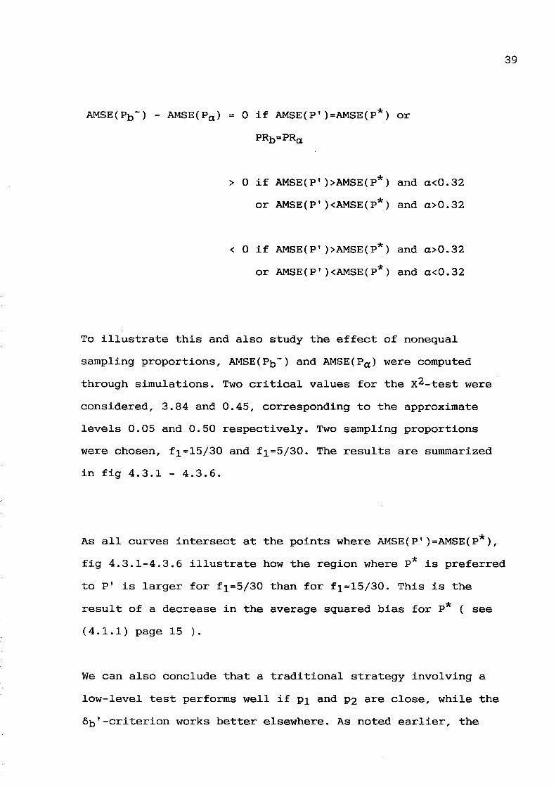
AMSE(Pb-) - AMSE(Pa ) = 0 if AMSE(P')=AMSE(P*) or

PRb=PRa

> 0 if AMSE(P'»AMSE(P*) and a<0.32

or AMSE(P')<AMSE(P*) and a>0.32

< 0 if AMSE(P' »AMSE(P*) and a>0.32

or AMSE(P')<AMSE(P*) and a<0.32

To illustrate this and also study the effect of nonequal

sampling proportions, AMSE(Pb-) and AMSE(Pa ) were computed

through simulations. Two critical values for the x2-test were

considered, 3.84 and 0.45, corresponding to the approximate

levels 0.05 and 0.50 respectively. Two sampling proportions

were chosen, fl=15/30 and fl=5/30. The results are summarized

in fig 4.3.1 - 4.3.6.

39

As all curves intersect at the points where AMSE(P')=AMSE(P*),

fig 4.3.1-4.3.6 illustrate how the region where p* is preferred

to p' is larger for f1=5/30 than for f1=15/30. This is the

result of a decrease in the average squared bias for p* ( see

(4.1.1) page 15 ).

We can also conclude that a traditional strategy involving a

low-level test performs well if P1 and P2 are close, while the

0b'-criterion works better elsewhere. As noted earlier, the

effect of increasing m, would be to reduce the region where p*

is preferred to P'. Thus, for larger m, the 0b'-criterion would

be better for a yet larger region.

In fig 4.3.4 and 4.3.6, we also note the non-symmetry for

AMSE(PO.05), when we have non-equal sampling proportions.

AMSE(PO.05) is larger for small values of PI than for large

values of Pl'

Fig 4.3.6 shows that AMSE(PO.50) actually is smaller than

AMSE(Pb') on the interval where AMSE(P*)<AMSE(P') if fl=5/30,

for the small values of PI and P2 covered in this figure.

40

41

4.4 Comparing Pb- with predictors based on the Akaike-

criterion.

The Akaike-criterion for choosing between two models, amounts

to comparing the quantities

and

where 11 and 12 are the maximized log-likelihood functions and

ql and q2 the number of estimated parameters of the models.

For our purposes we let 11 be the maximized log-likelihood

function under the hypothesis of homogenity

* * ~ ( Xlj·ln(p ) + (nj - Xlj)·ln(l-p ) )

and under the global alternative hypothesis we get

The Akaike-criterion states that we should use the predictor pI

if

Equivalently we may express this in terms the likelihood

functions, L1 and L2:

For the two-population case q2-q1=1, so we obtain

42

Since 2·ln(L2/L1) has an approximate chi-square

nulldistribution with one degree of freedom, this criterion is

approximately equivalent to adopting a likelihood ratio test on

the level of 0.16.

Let PA be the predictor defined by the rule

In fig 4.4.1 - 4.4.4 AMSE(Pb-) is compared with AMSE(PA).

We see that PA performs slightly better in the region where

ob<l, corresponding to values of PI and P2 quite close, while

Pb- is better elsewhere.

43

4.5 Effects of different sampling proportions in the old and

the new sample.

In so far we have assumed that the sampling proportions in the

old sample were identical to the proportions in the new sample,

for which we wanted to make predictions. This assumption

simplified the computations for AMSE(P') and AMSE(P*). In this

section we shall give a brief indication to what happens if

this assumption is not fulfilled. Let

ej mj/m, i.e. the proportion of obs. at Z=j

in the old sample, j=1,2, .•. ,k

fj = nj/n, i.e. the proportion of obs. at Z=j

in the new sample, j=1,2, ••• ,k

The AMSE:s are defined by averaging over the new sample as

usual

AMSE(P') =

AMSE(P*)

44

Evaluating MSE(Pj') and MSE(Pj*) for the proportions ej, we get

AMSE(P')

AMSE(P*)

where n

Studying AMSE(P*) for the case where k=2, we obtain

AMSE(P*)

AMSE(P*) - AMSE(P*) = (1 - 2·e1)·(e1 - f1)·(P1 - P2)2

e1=f1 e1+f 1

e.i. if P1+P2 we are better off if we try to predict for the

new sample, where f1Te1 if e1<0.5 and f1<e1 or e1>0.5 and

f1>e1. As is seen from fig 4.5.1, in the majority of cases we

are however worse off. Note that we can't interpret fig 4.5.1

45

as indicating the effect of e1 for a given fl. For example, if

f1=0.9, we can't say that AMSE(P*) is smaller for e1=0.6, say,

than for e1=0.9. For the latter problem we can minimize

AMSE(P*)

with respect to e1. Taking derivative we obtain

Restricting attention to the case P1+P2, for P1=P2 AMSE(P*)

don't depend on either e1 or f1, we put this equal to zero and

solve for e1.

46

As the second derivative is equal to 4·(P1-P2)2>0, the solution

is a minimum. It is seen that e1=f1 if the variances are equal

in the two populations. On the other hand, if the variance

P1·(1-P1) is large compared to P2·(1-P2), the minimal e1 is

smaller than fl.

47

Study the inequality

AMSE(P') - AMSE(P') = (1 - f1/e1)"P1"(1-P1) +

e1=f1 e1=ff1

> 0

For e1=ff1 we get two cases

AMSE(P') - AMSE(P') > 0 <=>

e1=f1 e1=ff1

AMSE(P') - AMSE(P') > 0 <=>

e1=f1 e1=ff1

P1"(1 - P1)

48

In fig 4.5.2 - 4.5.4, the regions in the (P1,P2)-space where

AMSE(P') - AMSE(P') > 0

e1=f1 e1+f 1

are shown, for values of e1 corresponding to 0.4, 0.5 and 0.6.

We see that for e1=0.5, the inequality is satisfied for exactly

half the space, both for f1>e1 and f1<e1. For e1=0.4 it is

satisfied for the larger region if f1<0.2 and for e1=0.6 if

f1>0.6.

It is clear that AMSE(Pb-), will be effected if e1+f1. This

effect should depend on the directions of the changes in

AMSE(P') and AMSE(P*). E.i. if both AMSE(P') and AMSE(P*) get

larger, then AMSE(Pb-) gets larger. This issue will not be

discussed further.

4.6 The multinomial case.

In the preceding sections, we have assumed that the sample

sizes for the different levels of Z, were fixed in advance,

both in the old and the new sample. E.i. we were dealing with

independent binomial sampling.

In this section we shall see that not much is changed for the

case where the sample sizes for different levels of Z are

random variables. We will assume that the total sample size is

fixed, e.i. multinomial sampling. As before we have the two

prediction rules p' and p*. We define

AMSE( P' )

AMSE(P*)

1: p '.E(p·'- p.)2 .J J J and

where P.j = P(Z=j) in the population where we want to make

predictions. Note that we keep the old notations for Pj' and

p*, but that they now have different distributions. After some

computations we get

AMSE(P*)

49

50

where P1.=P(Y=1). For AMSE(Pl) we rely on an approximation for

computing V(pj') (the de1tha-method, see appendix):

so

AMSE( PI) E Pj' (l-Pj )/m

Now, we would prefer the prediction rule pI if

E P ··p··(l-p·)/m + (m+1)E p "(P'-P1 )2/m - E p··(l-p·)/m > 0 .J J J .J J. J J

e.i. if

> 1

E (1 - P ')'p"(l - p.) • J J J

So om is practically equal to 0b' To estimate om, we insert the

M-L-estimates of the parameters (see appendix), and obtain:

Om' --------------------------- > 1

1: (1 - P ·')·p·'·(l - P") .J J J

where P.j' = x.j/m, the proportion of observations at Z=j, in

the old sample. Applying the prediction rule

Use P' if om' > 1

Use p* if om' ~ 1

and call this rule Pm'. Putting PR(om'>l), The AMSE of Pm' can

be written as

AMSE(Pm') = PRm·AMSE(P') + (1 - PRm)·AMSE(P*)

As in the binomial case this is an average of AMSE(P') and

AMSE(P*). Thus Pm' can be expected to perform well over large

regions of the parameter space.

51

Fig 4.1.3 Values of Pl and P2 where Oh = 1.

t.o o.t I .. 0.1

Pi

f1 = 5/30: -, f1 = 15/30 --­and P2=0.2-P1 are also indicated.

0.. 0.7 0.1 t.o

53

Fig 4.1.1 Comparison of AMSE(P') and AMSE(P*) for P2=1~Pl. 52

0.025

0.020

0.015

0.010

/ I

I I

I I

I 0.005 I

I I

I I

I

I I I I I I I I I I I I I I , I I I I I I I I I I I , ,

......... ",..... \

", \-", ,

", \ / \

/ \ / \

/ \

/ \ / \

/ \ / II

, , , , , , , , , , , , , , , , , , , , , , , , , , , ... ' t-.......... , "­, "-, "-: " , "

I " " " / , I , " \ ... \

\ \

\ \

\ \ \ \ \ \ \

o.ooo~~~TT~~rr~~rrTT~rrTT~rrrT~~rT~~rT~~~TT~~~\~· 0.0 0.1 0.2 o.s 0." 0,5 0.6 0.7 0.8 0.9 1.0

Pi

AMSE( P' ) :---, AMSE( p*) f1 =5/30 :--- AMSE( p*) f1 =15/30: _

Fig 4.1.2 Comparison of AMSE(P') and AMSE(P*) for P2=0.5-Pl.

0.030

0.025

0.020

0.015

0.010

0.005

\ \ \ \ \ \ \ \ \ \ \ \ \ \ \ \ \ \ \ \ \ \ \ \ \ \ \ \ \

\ \ \ \ \ ,

\ \ ,

--~ _ - I _ - I -- \ - \ ........... I

,*'" 'II,", ...... , ' ....

--' ,-,,;'

, ..

, , , , , , , , , , , , , , , , , , I

I , , , I ,

I I

I , I , ,

I I

I I

I

---L I - _ I - _

I -_ I ......

" ' ...... " ... ,

O.OOO~~~~~~~TT~~rT~~rrTT~~rT~~rrTT~~rT~-rrT~1 0.00 0.05 0.10 0.15 0.20 0.25 0.30 0.35 0.40 0.45 0.150

Pi

AMSE( P' ) : ---, AMSE( P*) f1 =5/30 :--- AMSE( p*) f1 =15/30: -

Fig 4.2.1 Comparison of AMSE(P')1 AMSE(P*) and AMSE(Pb-)· for fl 15/30 and P2 Pl·

0.020

0.015

0.010

0.005

0.020

0.015

0.010

0.005

-------------,- \

" \ ", \ ,/ \

" \ " \ , \

;' \ / \

\ I \ I ',--/

0.0 0.1 0.2 0.3 0.4 0.5

Pi

AMSE( P' ): - __

Fig 4.2.2 Comparison of AMSE(P'), AMSE(P*) and AMSE(Pb-) for fl-5/30 and P2=1-Pl.

, I I I I I I I I I I

_------_ I -- ................ I

I I

I I

I I

I I

I , / , / ,---/

0.0 0.1 0.2 0.3 0.4 0.5 0.6 0.7 0.8 0.9

Pi

AMSE(P' ):--- , AMSE(P*):- __ , AMSE(Pb-):_

54

1.0

Fig 4.3.1 (P AMSE(PO O ~) and AMSE(Pb-) Comparison of AMSE 0.50a'L ~ _

0.025

0.020

0.015

0.010

0.005

for f)-15/30 an P2 1-p).

0.0 0.1

".-, I ,

I \ I \

I \ I \

I \ I \

I \ I \

I \ I \

I \ I \ I \

I \ I \

I \ I \ I \

I \ I \ " /..--~\

I ./ I ./

I ./ I ./ " ./ I ./

I ./ I Y " ~ I

I I

I I

I I ,

0.2 0.3 0.4 0.5 0.6

Pi

AMSE(PO.50) :-__ , AMSE(PO.05):--- ,

, , \

\ \ \ \ \ \ \ \ \ \ \ \ \ \ \

0.7

\ \ \ \ \ \ \ \ \ \ \ \

0.8

\ \ \ \ \ \ \ \

\ \

\ \

\

0.9

AMSE(Pb-):-

1.0

Fig 4.3.2 Comparison of AMSE(Po 50), AMSE(Po 05) and AMSE(Pb-) for f]=5/30 and P2=1-P2.

0.030

0.025

0.020

0.015

0.010

0.005

0.0

..... - .... , " ... I ...

I \ I \

I \ I \

I \ I \

I \ I \

I \ I \

I \ I ,

" \ I I

I I

I I

I I

I I

I I

I I

I I

I I

I I

I I

I I.

0.1 0.2 0.3 0.4 0.5 0.6

Pi

AMSE( PO. 50): --- , AMSE (PO. 05) : - --

,,'- .... " ... I \ I \

I \ I \

I , I \

I \ I \

I , I ,

I , I \

I , I ,

,

0.7 0.8

, , , , \ \ , , , , ,

\ , , \ , , , ,

\ \

\ ,

0.9

\ ,

AMSE(Pb -): _

1.0

55

56

Fig 4.3.3 Comparison of AMSE(PO.SO), AMSE(PO.Os) and AMSE(Pb-) for fJ 15/30 and P2 0.5 Pl·

0.025

0.020

0.015

0.010

0.005

........ -- ....... , , " , " , " , " , , , , , , , , , ,

I , , , , , , , " ..,.,.------......; \

" "'""'""'" I "'" , "'" , "'" ....

0.00 0.05 0.10 0.15

~. "'" , ............. ..",/ ,~

" ....... -..--~" " , , " , " , " ,

0.20

", --"," ............ _-

0.25

Pi

0.30

"",.-- .......... , , " , " , " , , , , , , , , , , , , , , \ , \ , \ , \ 1.,.---....... \

....................... \

0.35 0.40

" \ " \ -..;:

0.45 0.50

AMSE(PO.50):---, AMSE(PO.05):--- , AMSE(Pb-):-

Fig 4.3.4 Comparison of AMSE(Po.so), AMSE(Po.os) and AMSE(Pb-) for f1-5/30 and P2=O.5-Pl.

0.025

0.020

0.010

0.005

~'---"'" , " , ,

, " , ,

//

/"'" ,... //"'"

0.00 0.05

, , , , , , , , , , , , , , , , ------'

0.10 0.15

.... _- ---

0.20 0.25 0.30 0.35

Pi

,---- .... ,

0.40

, , , , , , , , , \

" \ " \

0.45

" "

0.50

AMSE(PO.50):--- , AMSE(PO .. 05):--- , AMSE(Pb-):-

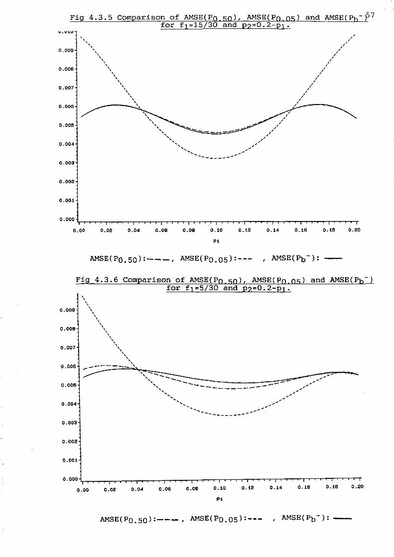
Fig 4.3.5 Comparison of AMSE(PO.50), AMSE(Po as) and AMS~(Pb-?7 for f,=15/30 and P2=0.2-p,.

v.V1U .. .. .. 0.009

0.008

0.007

0.006

0.005

0.004

0.003

0.002

0.001

0.00

.. , , , , , , , , , , , , , , , , , , , , , , ---- "

0.02 0.04

, , , , , .. .. .. .. .. ..

0.06

.. .. .. .. .............. ---

0.08 0.10 0.12

Pi

AMSE(PO.50) :---, AMSE(PO.05) :---

/ / ,

/ , /

/ , / , , , ,

/ /

/ /

/ /_----

0.14 0.16 0.18

/ /

/ /

,. ,. ,.

/

0.20

Fig 4.3.6 Comparison of AMSE(Po.sO), AMSE(PO.os) and AMSE(Pb-) for f1=5/30 and P2=0.2-P1.

, , , 0.009

0.008

0.007

, , , , , , , , , , , , , , , , , , , , , .. .. 0.006 ."",..------ ,

0.005

0.004

0.003

0.002

0.001

0.00 0.02 0.04 0.06 0.08 0.10 0.12

Pi

AMSE(PO.50):---, AMSE(PO.05):---

0.14 0.16 0.18 0.20

0.025

0.020

0.015

0.010

0.005

0.00

0.025

0.020

0.015

0.010

0.005

I ,

0.00

, , , ,

, ,

Fig 4.4.1 Comparison of AMSE(PA) and AMSE(Pb-)

for f1=15/30, P2=0.5-P1·

... .. .... _---'

0.05 0.10 0.15 0.20 0.25

Pi

.-.-, , ,

.­, , ,

0.30 0.35 0.40 0.45

Fig 4.4.2 Comparison of AMSE(PA) and AMSE(Pb-) for fJ-5/30, P2-0.5-PJ.

.-, .-.... .-

0.05 0.10 0.15

------

0.20 0.25 0.35 0.40 0.45

Pi

58

0.50

0.50

0.005

0.00

0.005

0.00

Fig 4.4.3 Comparison of AMSE(PA) and AMSE(Ph-) , 59 for f1=15/30, P2-0 .2-Pl·

------------ .~---- ..

0.02

0.02

Pi

Fig 4.4.4 Comparison of AMSE(PA) and AMSE(Ph-) for f]-5/30, P2=0.2-Pl.

---------------

0.06 0,08 0.10 0.12 0.14 0.16 0.18

Pi

AMSE(PA): -- - , AMSE(Pb -):_

" ,.

0.20

Fig 4.5.1 Effects of different sampling proportions in the old - * and the new sample for AMSE(P ).

F1 1.0+-------------r------------'/I

0.9

0.8

0.7

0.6

0.6

0."

0.3

0.2

0.1

O.O~--_r----r_--_r--~r_--~--_,----._--_.----._---T

0.0 0.1 0.2 0.3 0." 0.6

E1

0.6 0.7 0.8 0.9 1.0

The shaded area indicates the values of f1 and e1 where AMSE(P*) for e1=f1 is larger than AMSE(P*) for e1+f1.

60

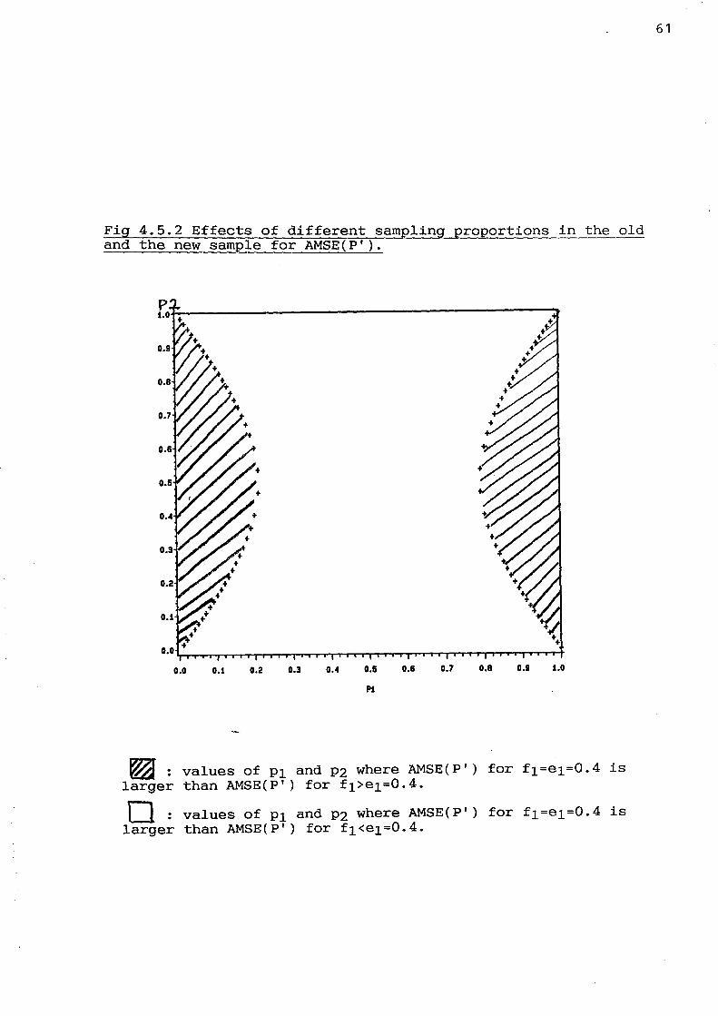
Fig 4.5.2 Effects of different sampling proportions in the old and the new sample for AMSE(P').

P 1.0~------------------------------------------------~

+

O.01,..+....,.. ................................................ ....-.....,..,....,..,.....,..,. ...... ...,..,. ............ ..,.....,..,.....,rnr-r-r-r-..-r-r-r-rr-r-... +r-++

0.0 0.1 0.2 0.3 0.4 0.6 0.& 0.7 0.& 0.9 1.0

Pl

~ : values of PI and P2 where AMSE(P') for f1=e1=0.4 is larger than AMSE(P') for f1>e1=0.4.

r:J : values of P1 and P2 where AMSE(P') for f1=e1=0.4 is larger than AMSE(P') for f1<e1=0.4.

61

and the new sample for AMSE(P').

F~ 4 ~ .5.3 Effects of different sam in the old

0.0 o.t 0.2 0.3 0.4 0.5 O.B 0.7 0.8 0.9 t.o

Pt

~ : values of P1 and P2 where AMSE(P') for f1=e1=0.5 is larger than AMSE(P') for f1>e1=0.5.

L:J : values of P1 and P2 where AMSE(P') for f1=e1=0.5 is larger than AMSE(P') for f1<e1=0.5.

62

Fig 4.5.4 Effects of different sampling proportions in the old and the new sample for AMSE(P' ).

0.0 0.1 0.2 0.3 0." 0.5 0.6 0.7 O.B 0.9 1.0

PI

~: values of P1 and P2 where AMSE(P') for f1=e1=0.6 is larger than AMSE(P') for f1>e1=0.6.

c=J: values of P1 and P2 where AMSE(P') for f1=e1=0.6 is larger than AMSE(P') for f1<e1=0.6.

64

5 Concluding remarks.

When making hypothesis testing, the rejection of a true null­

hypothesis is usually considered to be a grave error. This

consideration calls for adopting a small significance level,

such as 0.05 or 0.01. When choosing between two prediction

rules, such as p* and pI, we don't have such prior

considerations. This paper has shown that if we adopt a low­

level significance test for choosing between p* and P' this

procedure has a high AMSE-risk for large areas of the parameter

space.

65

APPENDIX: Collection of some useful results.

AI. MSE(Pj*) and MSE(Pj') for the multinomial case.

We begin by evaluating MSE(Pj*)' for the multinomial case. We

have that

* MSE(Pj )

Here we have used the fact that xl. has a binomial distribution

with parameters Pl. and n.

We proceed by considering MSE(Pj')

+ (E(XIO/X 0) _ po)2 J.J J

Now, for the expectation of Pj' we have

66

EE(Xlj/X.j I x.j) = E(Pj) = Pj

By adopting the multivariate deltha method we will evaluate an

approximation to the variance of Pj'. We first formulate the

method in general terms. Let e=(el, ••• ,et)' be a vector of

parameters and let en'=(enl', ••• ,ent')' be a vector of random

variables with the same dimension. Assume that en' has an

asymptotic normal distribution in the sense that

L(n·(en ' - e» ~ N(O, E(e»

where L stands for convergence in distribution and E(e) is the

asymptotic covariance matrix of en'. Further, let f be a

function which has the following expansion as x~e

f(x) fee) + (x-e)De' + o(~x-e~)

67

where De is the vector of partial derivatives of f evaluated at

x=e. Within this framework, the asymptotic distribution of

f(en ') is given by

68

L(n·(f(Sn') - f(S») ~ N(O, DSE(S)DS')

We proceed by determining the asymptotic variance of PI' for a

2x2 -table, the argument being the same for P2'. Put

f(Sn') f(S) = Pll/p.1 = PI

It is well-known that the Xij:s have an asymptotic normal

distribution and the asymptotic covariance matrix is given by

E(S)

Computing the elements of De

P2l

of/oenl' = ------­

m·p.l2

Pll

of/oen3'= - -------

m·p.l2

As f(en ') does not include e n2' and e n4' the dimension of De is

2xl. This implies that the asymptotic variance of Pl' is given

by

m·De De'

Performing this computation we arrive at

69

70

A2. Maximum-likelihood estimators for the multinomial case.

Here we derive the M.L-estimators of the probabilities Pj , Pl.

and P.j , j=1,2, ••. ,k, for the multinomial case. The likelihood

function for the 2xk random variables is

m!

L =

TtTtXij!

TtTtp' .x ~J

The essential part of the log-likelihood function is

i = 0,1 j 1,2, ... ,k

Writing out the summation over the index i we get

Making the substitution P1j=Pj·P.j

1 I: (xO' ·log( P . - P .• P .) + xl' ·log( P .. P . » J .J .J J J .J J

Maximizing this with respect to Pj by taking derivative and

putting this equal to zero

Xlj·p.j/Pj·p.j - XOj·p.j/(p.j-p.j·Pj) = 0

<=>

Pj xlj/x.j

For the probabilities P.j, we observe that under this sampling

plan the vector (X. I, x.2, ••• ,x.k)' has a multinomial

distribution with parameters m=x .• and P.I, P.2, ... ,P.k. We

therefore conclude that the M.L-estimator of P.j is x.j/m.

By a similar reasoning we also conclude that the M.L-estimator

of Pl. is given by xI./m.

71

REFERENCES

Aitkin, M. (1978): A Simultaneous Test Procedure for

Contingency Table Models, J. Roy. Statist. Soc. (C) 141,

195-223

Atkinson, A.C. (1980): A Note on the Generalized Information

Criterion for Choice of a Model, Biometrika, 67, 413-418

Benedetti, J.K and Brown, M.D. (1976): Alternate Methods of

Building Log-Linear Models, Proceedings of the 9th

International Biometric Conference, The Biometric Society,

209-227

Efron, B (1978): Regression and ANOVA with Zero-One Data, JASA,

73, 113-121

Efron, B. (1986): How Biased is the Apparent Error Rate of a

Prediction Rule? JASA, 81, 461-470

Fowles, e.b., Freeny, A.E., and Landwehr, J.M. (1988):

Evaluating Logistic Models for Large Contingency Tables, JASA,

83, 611-622

Goodman, L.A. (1964): Simultaneous Confidence Limits for Cross­

Product Ratios in Contingency Tables, J. Roy. Statist. Soc.

(B), 26, 86-102

Hildebrand, O.K., Laing, 1.0. and Rosenthal, H. (1977):

Prediction Analysis of Cross Classifications, John Wiley &

Sons, New York

van Houwelingen, J.C. and Le Cessie, S. (1989): Predictive

Value of Statistical Models, Proceedings of the Compo Stat.

Conf. Copenhagen, 1988

Linhart, H. and Zucchini, W. (1986): Model Selection, John

Wiley & Sons, New York

1990:1

1990:2

1991:1

Holm, s.

Holm, s. & Dahlbom, U

Olofsson, Jonny

Abstract bootstrap confidence intervals in linear models.

On tests of equivalence

On some prediction methods for categorical data