On some identities involving exponentials

Fernando CasasFernando.Casas@mat.uji.es

www.gicas.uji.es/Fernando/fernando.html

Departament de MatematiquesInstitut de Matematiques i Aplicacions de Castello (IMAC)

Universitat Jaume ICastellon

ICMAT, May 2015

Based on work done (along the years) with

Ander Murua

Sergio Blanes

Jose Ros

Jose Angel Oteo

0. INTRODUCTION

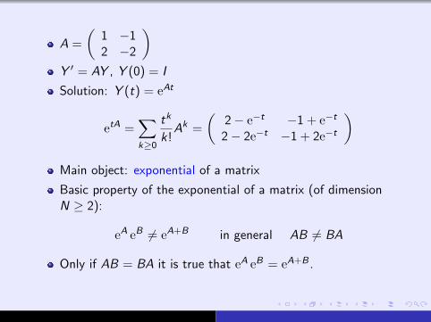
A =

(1 −12 −2

)Y ′ = AY , Y (0) = I

Solution: Y (t) = eAt

etA =∑k≥0

tk

k!Ak =

(2− e−t −1 + e−t

2− 2e−t −1 + 2e−t

)Main object: exponential of a matrix

Basic property of the exponential of a matrix (of dimensionN ≥ 2):

eA eB 6= eA+B in general AB 6= BA

Only if AB = BA it is true that eA eB = eA+B .

A trivial example

Consider

A =

(1 10 1

)and B =

(1 01 0

)A and B do not commute:

AB =

(2 01 0

)and BA =

(1 11 1

)Hence we have

eA =

(e e0 e

)and eB =

(e 0

e− 1 1

)

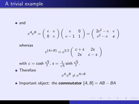
A trivial example

and

eAeB =

(e e0 e

)(e 0

e− 1 1

)=

(2e2 − e ee2 − e e

)whereas

e(A+B) = e3/2

(c + s 2s

2s c − s

)with c = cosh

√5

2 , s = 1√5

sinh√

52 .

ThereforeeA eB 6= eA+B

Important object: the commutator [A,B] = AB − BA

Problems

1 eA eB = eA+B+C

2 eA+B = eA eB eC1 eC2 . . .3 Given Y ′ = A(t)Y , Y (0) = I , with A(t) a N × N matrix,

N = 1: Y (t) = e∫ t

0A(s)ds

N > 1: Y (t) = e∫ t

0A(s)ds if[

A(t),

∫ t

0

A(s)ds

]= 0 (Coddington & Levinson)

General case: can we write Y (t) = eΩ(t) with

Ω(t) =

∫ t

0

A(s)ds + (something else)?

Motivation

Exponential map:

Fundamental role played by the exponential transformation inLie groups and Lie algebras

exp : g 7−→ G

Kashiwara–Vergne conjecture (with important implicaciones inLie theory, harmonic analysis, etc.), proved as a theorem in2006

Lie groups are ubiquitous in physics: symmetries in classicalmechanics, Quantum Mechanics, control theory, etc.

I. MAIN CHARACTERS

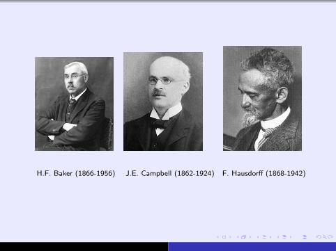
H.F. Baker (1866-1956) J.E. Campbell (1862-1924) F. Hausdorff (1868-1942)

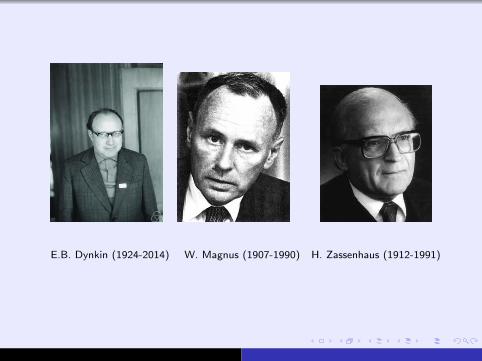
E.B. Dynkin (1924-2014) W. Magnus (1907-1990) H. Zassenhaus (1912-1991)

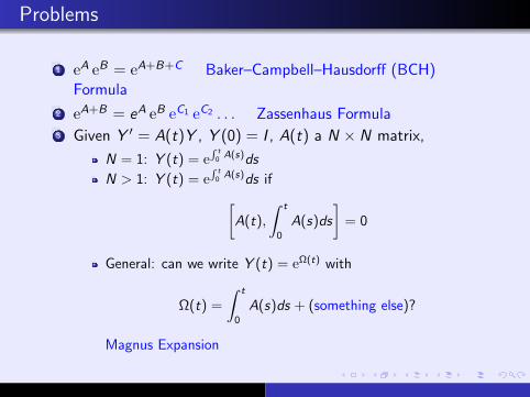
Problems

1 eA eB = eA+B+C Baker–Campbell–Hausdorff (BCH)Formula

2 eA+B = eA eB eC1 eC2 . . . Zassenhaus Formula3 Given Y ′ = A(t)Y , Y (0) = I , A(t) a N × N matrix,

N = 1: Y (t) = e∫ t

0A(s)ds

N > 1: Y (t) = e∫ t

0A(s)ds if[A(t),

∫ t

0

A(s)ds

]= 0

General: can we write Y (t) = eΩ(t) with

Ω(t) =

∫ t

0

A(s)ds + (something else)?

Magnus Expansion

These topics have already appeared (several times) at the workshopWe are mainly concerned by

computational aspects: how to generate efficiently thecorresponding series

Convergence of the series

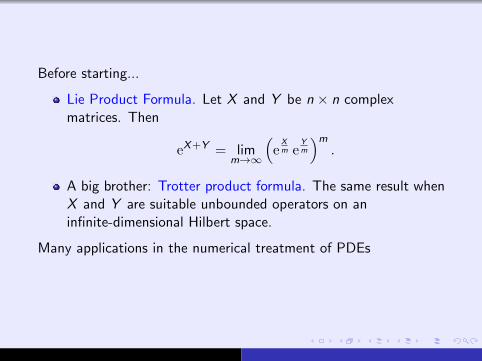
Before starting...

Lie Product Formula. Let X and Y be n × n complexmatrices. Then

eX+Y = limm→∞

(e

Xm e

Ym

)m.

A big brother: Trotter product formula. The same result whenX and Y are suitable unbounded operators on aninfinite-dimensional Hilbert space.

Many applications in the numerical treatment of PDEs

II. BCH FORMULA

eX eY = eZ

Let X , Y be two non commuting operators. Then

eX eY =∞∑

p,q=0

1

p! q!X p Y q

Substituting this series in the formal series defining thelogarithm function

logZ =∞∑k=1

(−1)k−1

k(Z − 1)k

one gets

Z = log(eX eY ) =∞∑k=1

(−1)k−1

k

∑ X p1Y q1 . . .X pkY qk

p1! q1! . . . pk ! qk !,

The inner summations extends over all non-negative integersp1, q1, . . . , pk , qk for which pi + qi > 0 (i = 1, 2, . . . , k).

First terms:

Z = (X + Y + XY +1

2X 2 +

1

2Y 2 + · · · )

− 1

2(XY + YX + X 2 + Y 2 + · · · ) + · · ·

= X + Y +1

2(XY − YX ) + · · · = X + Y +

1

2[X ,Y ] + · · ·

Baker, Campbell, Hausdorff analyzed whether Z can bewritten as a series only in terms of (nested) commutators

The answer is yes, but they weren’t able to provide a rigorousproof

Bourbaki: “chacun considere que les demonstrations de sespredecesseurs ne sont pas convaincantes”

Finally, Dynkin (1947): explicit formula for Z .

Sometimes it is called BCH-D (for Dynkin) formula(Bonfiglioli & Fulci)

Dynkin:

Z =∞∑k=1

∑pi ,qi

(−1)k−1

k

[X p1Y q1 . . .X pkY qk ]

(∑k

i=1(pi + qi )) p1! q1! . . . pk ! qk !(1)

Inner summation over all non-negative integers p1, q1, . . ., pk ,qk for which p1 + q1 > 0, . . . , pk + qk > 0

[X p1Y q1 . . .X pkY qk ] denotes the right nested commutatorbased on the word X p1Y q1 . . .X pkY qk :

[XY 2X 2Y ] ≡ [X , [Y , [Y , [X , [X ,Y ]]]]]

Gathering terms together

Z = log(eX eY ) = X + Y +∞∑

m=2

Zm, (2)

Zm(X ,Y ): homogeneous Lie polynomial in X , Y of degree m,i.e., a Q-linear combination of commutators of the form[V1, [V2, . . . , [Vm−1,Vm] . . .]] with Vi ∈ X ,Y for 1 ≤ i ≤ m.

First terms

Z2 =1

2[X ,Y ]

Z3 =1

12[X , [X ,Y ]]− 1

12[Y , [X ,Y ]]

Z4 = − 1

24[Y , [X , [X ,Y ]]]

Z5 =1

720[X , [X , [X , [X ,Y ]]]]− 1

180[Y , [X , [X , [X ,Y ]]]]

+1

180[Y , [Y , [X , [X ,Y ]]]] +

1

720[Y , [Y , [Y , [X ,Y ]]]]

− 1

120[[X ,Y ], [X , [X ,Y ]]]− 1

360[[X ,Y ], [Y , [X ,Y ]]]

Applications

Fundamental role in different fields:

Mathematics: theory of linear differential equations, Liegroups, numerical analysis of differential equations

Theoretical Physics: perturbation theory, quantum mechanics,statistical mechanics, quantum computing

Control theory: design and analysis of nonlinear controlmechanisms, nonlinear filters, stabilization of rigid bodies,...

Applications

Quantum Mechanics

i~U = HU(t), U(t0) = I , so that ψ(t) = U(t)ψ0

H(t) = K + V = − ~2

2mp2 + V

Solution: U(t) = e−iHt/~.

Very often, computing e−iKt/~, e−iVt/~ is easier

Applications

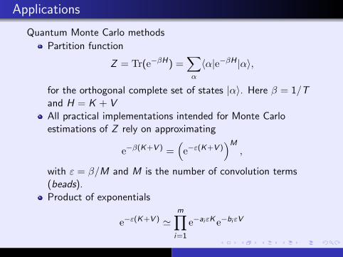
Quantum Monte Carlo methods

Partition function

Z = Tr(e−βH) =∑α

〈α|e−βH |α〉,

for the orthogonal complete set of states |α〉. Here β = 1/Tand H = K + VAll practical implementations intended for Monte Carloestimations of Z rely on approximating

e−β(K+V ) =(e−ε(K+V )

)M,

with ε = β/M and M is the number of convolution terms(beads).Product of exponentials

e−ε(K+V ) 'm∏i=1

e−aiεKe−biεV

Applications

Lie groups theory: Lie algebra ↔ Lie group. Multiplicationlaw in the group is determined uniquely by the Lie algebrastructure, at least in a neighborhood of the identity

Helpful also to prove the existence of a local Lie group with agiven Lie algebra

The particular structure of the series is not very important inthis setting...

...But in other fields it is relevant to analyze the combinatorialaspects and its efficient computation

Applications

Lie groups theory: Lie algebra ↔ Lie group. Multiplicationlaw in the group is determined uniquely by the Lie algebrastructure, at least in a neighborhood of the identity

Helpful also to prove the existence of a local Lie group with agiven Lie algebra

The particular structure of the series is not very important inthis setting...

...But in other fields it is relevant to analyze the combinatorialaspects and its efficient computation

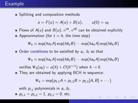
Example

Splitting and composition methods

u = F (u) = A(u) + B(u), u(0) = u0

Flows of A(u) and B(u), etA, etB can be obtained explicitly

Approximation (for t = h, the time step)

Ψh ≡ exp(ha1A) exp(hb1B) · · · exp(hakA) exp(hbkB)

Order conditions to be satisfied by ai , bi so that

Ψh ≡ exp(ha1A) exp(hb1B) · · · exp(hakA) exp(hbkB)

verifies Ψh(u0) = u(h) +O(hr+1) when h→ 0.

They are obtained by applying BCH in sequence:

Ψh = exp(p1,1A + p1,2B + p2,1[A,B] + · · · )

with pi ,j polynomials in ai , bi .

p1,1 = p1,2 = 1, p2,1 = 0, etc.

How to obtain the BCH formula

Different procedures in the literature:Goldberg form + Dynkin (Specht-Wever) theorem (explicit)

Z = X + Y +∞∑n=2

1

n

∑w ,|w |=n

gw [w ], (3)

with w = w1w2 . . .wn, each wi is X or Y ,[w ] = [w1, [w2, . . . [wn−1,wn] . . .]], the coefficient gw is arational number and n is the word length.Varadarajan (recursive)

Z1 = X + Y (4)

(n + 1)Zn+1 =1

2[X − Y ,Zn] +

[n/2]∑p=1

B2p

(2p)!∑[Zk1 , [· · · [Zk2p ,X + Y ] · · · ]], n ≥ 1

Second sum: over all positive integers such thatk1 + · · ·+ k2p = n

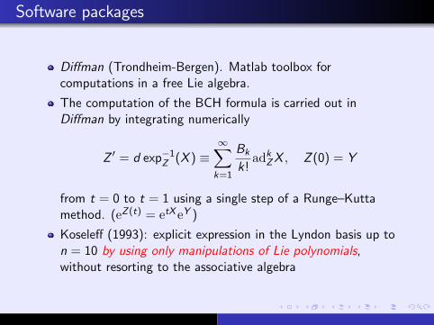
Software packages

Diffman (Trondheim-Bergen). Matlab toolbox forcomputations in a free Lie algebra.

The computation of the BCH formula is carried out inDiffman by integrating numerically

Z ′ = d exp−1Z (X ) ≡

∞∑k=1

Bk

k!adkZX , Z (0) = Y

from t = 0 to t = 1 using a single step of a Runge–Kuttamethod. (eZ(t) = etX eY )

Koseleff (1993): explicit expression in the Lyndon basis up ton = 10 by using only manipulations of Lie polynomials,without resorting to the associative algebra

Software packages

Reinsch (2000): Simple derivation with matrices of rationalnumbers. Mathematica program. The expression is notwritten in terms of commutators

A recent (much simpler) modification in 2015

Lie Tools Package (LTP) (Torres-Torriti & Michalska, 2003).

Package in Maple for carrying out Lie algebraic symboliccomputations.Special function for the computation of BCH formula in theDynkin form in terms of Lie monomials in the Hall basis.Reported results in 2003: up to order 10 in 25 hours withmaximum memory usage of 17.5 Mbytes on a Pentium III, 550MHz, 256 Mbytes RAM, Maple 7, Linux

Bottleneck in the computation

The iterated commutators are not all linearly independent,due to the Jacobi identity

[X1, [X2,X3]] + [X2, [X3,X1]] + [X3, [X1,X2]] = 0

(and other identities involving nested commutators of higherdegree originated by it)

All the previous expressions for the BCH series are notformulated directly in terms of a basis of the free Lie algebraL(X ,Y )

Problematic when designing numerical integrators for ODEs(one condition per element in the basis)

Very difficult to study specific properties of the series:distribution of coefficients, combinatorial properties, etc.

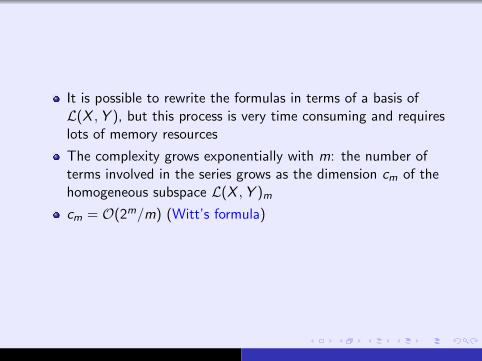
It is possible to rewrite the formulas in terms of a basis ofL(X ,Y ), but this process is very time consuming and requireslots of memory resources

The complexity grows exponentially with m: the number ofterms involved in the series grows as the dimension cm of thehomogeneous subspace L(X ,Y )m

cm = O(2m/m) (Witt’s formula)

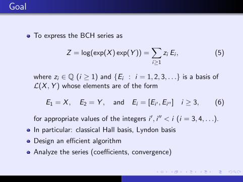
Goal

To express the BCH series as

Z = log(exp(X ) exp(Y )) =∑i≥1

zi Ei , (5)

where zi ∈ Q (i ≥ 1) and Ei : i = 1, 2, 3, . . . is a basis ofL(X ,Y ) whose elements are of the form

E1 = X , E2 = Y , and Ei = [Ei ′ ,Ei ′′ ] i ≥ 3, (6)

for appropriate values of the integers i ′, i ′′ < i (i = 3, 4, . . .).

In particular: classical Hall basis, Lyndon basis

Design an efficient algorithm

Analyze the series (coefficients, convergence)

Summary of the algorithm

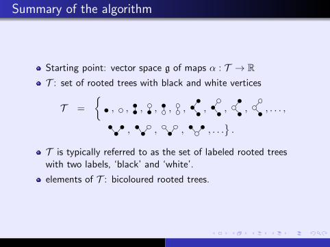
Starting point: vector space g of maps α : T → RT : set of rooted trees with black and white vertices

T =

, , , , , , , , , , . . . ,

, , , , . . ..

T is typically referred to as the set of labeled rooted treeswith two labels, ‘black’ and ‘white’.

elements of T : bicoloured rooted trees.

g is endowed with a Lie algebra structure by defining the Liebracket [α, β] ∈ g, of two arbitrary maps α, β ∈ g as

For each u ∈ T ,

[α, β](u) =

|u|−1∑j=1

(α(u(j))β(u(j))− α(u(j))β(u(j))

), (7)

|u| denotes the number vertices of u

each of the pairs of trees (u(j), u(j)) ∈ T × T ,

j = 1, . . . , |u| − 1, is obtained from u by removing one of the|u| − 1 edges of the rooted tree u, the root of u(j) being theoriginal root of u.

For instance

[α, β]( ) = α( )β( )− α( )β( ), [α, β]( ) = 0

[α, β]( ) = 2(α( )β( )− α( )β( )

)[α, β]( ) = α( )β( ) + α( )β( )

−α( )β( )− α( )β( )

The Lie subalgebra of g generated by the maps X ,Y ∈ gdefined as

X (u) =

1 if u =0 if u ∈ T \ , Y (u) =

1 if u =0 if u ∈ T \ (8)

is a free Lie algebra over the set X ,Y L(X ,Y ): Lie subalgebra of g generated by the maps X and Y .

For each particular Hall–Viennot basis Ei : i = 1, 2, 3, . . .,and X and Y as above, one can associate a bicoloured rootedtree ui to each element Ei such that, for any mapα ∈ L(X ,Y ),

α =∑i≥1

α(ui )

σ(ui )Ei , (9)

For each i , σ(ui ) is certain positive integer associated to thebicoloured rooted tree ui (the number of symmetries of ui )

if α ∈ L(X ,Y ), then its projection αn to the homogeneoussubspace L(X ,Y )n is given by

αn(u) =

α(u) if |u| = n0 otherwise

(10)

for each u ∈ T .

Lie series:

α = α1 + α2 + α3 + · · · , where αn ∈ L(X ,Y )n.

A map α ∈ g is then a Lie series if and only if (9) holds

The corresponding BCH series is a Lie series

Z =∑i≥1

ziEi =∑i≥1

Z (ui )

σ(ui )Ei

= Z ( )X + Z ( )Y + Z ( )[Y ,X ]

+Z ( )

2[[Y ,X ],X ] + Z ( )[[Y ,X ],Y ] + · · · ,

The coefficients Z (ui ) can be determined by recursiveprocedures for BCH (Varadarajan)

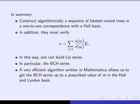
In summary:

Construct algorithmically a sequence of labeled rooted trees ina one-to-one correspondence with a Hall basis

In addition, they must verify

α =∑i≥1

α(ui )

σ(ui )Ei ,

In this way, one can build Lie series

In particular, the BCH series

A very efficient algorithm written in Mathematica allows us toget the BCH series up to a prescribed value of m in the Halland Lyndon basis

Some results

Comparison:

with the best previous algorithm: 17.5 MBytes up to m = 10.ours: 5.4 MBytes

In less than 15 min. of CPU (2008) and 1.5 GBytes we get upto m = 20

109697 non vanishing terms out of 111013 elements Ei ofgrade |i | ≤ 20 in the Hall basis

Last element:

E111013 = [[[[[Y ,X ],Y ], [Y ,X ]], [[[Y ,X ],X ], [Y ,X ]]],

[[[[Y ,X ],Y ], [Y ,X ]], [[[[Y ,X ],Y ],Y ],Y ]]],

with coefficient

z111013 = − 19234697

140792940288.

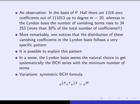
An observation: In the basis of P. Hall there are 1316 zerocoefficients out of 111013 up to degree m = 20, whereas inthe Lyndon basis the number of vanishing terms rises to 34253 (more than 30% of the total number of coefficients!!)

More remarkably, one notices that the distribution of thesevanishing coefficients in the Lyndon basis follows a veryspecific pattern

It is possible to explain this pattern

In a sense, the Lyndon basis seems the natural choice to getsystematically the BCH series with the minimum number ofterms

Variations: symmetric BCH formula

e12X eY e

12X = eW

Convergence

Theorem

(Mityagin) The Baker–Campbell–Hausdorff series convergesabsolutely when ‖X‖+ ‖Y ‖ < π.

This result can be generalized to any set X1,X2, . . . ,Xk ofbounded operators in a Hilbert space H:

eX1eX2 · · · eXk = eZ

converges if

‖X1‖+ ‖X2‖+ · · ·+ ‖Xk‖ < π

Optimal bound

An example

Let

X1 =

(1 00 −1

), X2 =

(0 10 0

)and let X = αX1, Y = β X2, with α, β ∈ C. Then

log(eX eY ) = αX1 +2αβ

1− e−2αX2,

analytic function for |α| < π with first singularities at α = ±iπ.Then BCH cannot converge if |α| ≥ π, independently of β 6= 0.

From the above theorem: convergence if |α|+ |β| < π

In the limit |β| → 0 this result is optimal

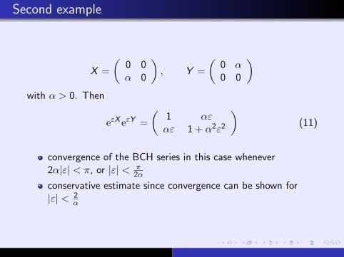
Second example

X =

(0 0α 0

), Y =

(0 α0 0

)with α > 0. Then

eεX eεY =

(1 αεαε 1 + α2ε2

)(11)

convergence of the BCH series in this case whenever2α|ε| < π, or |ε| < π

2α

conservative estimate since convergence can be shown for|ε| < 2

α

Numerical check of convergence for α = 2

Z [N](ε) =∑N

n=1 Zn(ε)

Compute Er (ε) = ‖eX eY e−Z [N](ε) − I‖Convergence if ε < 1

ε = 1/4; with N = 10, Er (ε) ≈ 10−7. With N = 15,Er (ε) ≈ 10−10

ε = 0.9; to get Er (ε) ≈ 10−8 we need N = 150; with N = 200then Er (ε) ≈ 10−10

Other results on convergence

The Baker–Campbell–Hausdorff formula expressed as a seriesof homogeneous Lie polynomials in X ,Y ∈ g (a Banach Liealgebra), converges absolutely in the domain D1 ∪D2 of g× g,where

D1 =

(X ,Y ) : µ‖X‖ <

∫ 2π

µ‖Y ‖

1

g(x)dx

D2 =

(X ,Y ) : µ‖Y ‖ <

∫ 2π

µ‖X‖

1

g(x)dx

and g(x) = 2 + x2 (1− cot x

2 ). (Michel 1974, F.C. & S. Blanes2004)

Biagi & Bonfiglioli 2014: generalization to arbitraryinfinite-dimensional Banach-Lie algebras (in particular,without using the exponential map)

III. ZASSENHAUS FORMULA

Zassenhaus formula

In the paper dealing with ME expansion, Magnus (1954) citesan unpublished reference by Zassenhaus, reporting that thereexists a formula which may be called the dual of the(Baker–Campbell–)Hausdorff formula. More specifically,

Theorem

(Zassenhaus Formula). Let L(X ,Y ) be the free Lie algebragenerated by X and Y . Then, eX+Y can be uniquely decomposedas

eX+Y = eX eY∞∏n=2

eCn(X ,Y ) = eX eY eC2(X ,Y ) · · · eCn(X ,Y ) · · · ,

where Cn(X ,Y ) ∈ L(X ,Y ) is a homogeneous Lie polynomial in Xand Y of degree n.

Zassenhaus formula

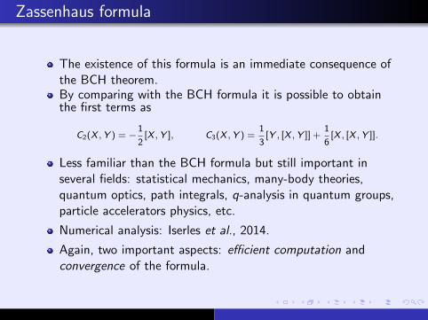
The existence of this formula is an immediate consequence ofthe BCH theorem.By comparing with the BCH formula it is possible to obtainthe first terms as

C2(X ,Y ) = −1

2[X ,Y ], C3(X ,Y ) =

1

3[Y , [X ,Y ]] +

1

6[X , [X ,Y ]].

Less familiar than the BCH formula but still important inseveral fields: statistical mechanics, many-body theories,quantum optics, path integrals, q-analysis in quantum groups,particle accelerators physics, etc.

Numerical analysis: Iserles et al., 2014.

Again, two important aspects: efficient computation andconvergence of the formula.

Some (brief) history

Several systematic computations of the terms Cn for n > 3have been carried out in the literature: Wilcox (1967), Volkin(1968), Suzuki (1976), Baues (1980). All of them give resultsfor Cn as a linear combination of nested commutators.Scholz and Weyrauch (2006): recursive procedure based onupper triangular matrices.Weyrauch and Scholz (2009): Cn up to n = 15 in less than 2minutes (with another procedure)Now

Cn =∑

w ,|w |=n

gw w , (12)

where gw is a rational coefficient and the sum is taken over allwords w with length |w | = n in the symbols X and Y , i.e.,w = a1a2 · · · an, each ai being X or Y .Applying Dynkin–Specht–Wever theorem it is possible toexpress them in terms of commutators, but in a way thatthere are redundancies

Our contribution

To present a new recurrence that allows one to express theZassenhaus terms Cn up to a prescribed degree directly interms of independent commutators involving n operators Xand Y .

We are able to express directly Cn with the minimum numberof commutators required at each degree n.

We obtain sharper bounds for the terms of the Zassenhausformula which show that the product converges in a largerdomain than previous results.

A new recurrence

We introduce a parameter λ,

eλ(X+Y ) = eλX eλY eλ2C2 eλ

3C3 eλ4C4 · · · (13)

so that the original Zassenhaus formula is recovered whenλ = 1.

Consider the compositions

R1(λ) = e−λY e−λX eλ(X+Y ) (14)

and for each n ≥ 2,

Rn(λ) = e−λnCn · · · e−λ2C2 e−λY e−λX eλ(X+Y ) = e−λ

nCn Rn−1(λ).

Then,Rn(λ) = eλ

n+1Cn+1 eλn+2Cn+2 · · ·

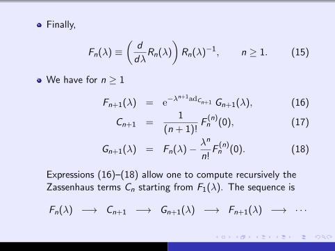
Finally,

Fn(λ) ≡(

d

dλRn(λ)

)Rn(λ)−1, n ≥ 1. (15)

We have for n ≥ 1

Fn+1(λ) = e−λn+1adCn+1 Gn+1(λ), (16)

Cn+1 =1

(n + 1)!F

(n)n (0), (17)

Gn+1(λ) = Fn(λ)− λn

n!F

(n)n (0). (18)

Expressions (16)–(18) allow one to compute recursively theZassenhaus terms Cn starting from F1(λ). The sequence is

Fn(λ) −→ Cn+1 −→ Gn+1(λ) −→ Fn+1(λ) −→ · · ·

For n = 1,F1(λ) = e−λadY (e−λadX − I )Y ,

that is,

F1(λ) =∞∑i=0

∞∑j=1

(−λ)i+j

i !j!adiY ad

jXY (19)

or equivalently

F1(λ) =∞∑k=1

f1,k λk , with f1,k =

k∑j=1

(−1)k

j!(k − j)!adk−jY adjXY .

(20)

In general (n ≥ 2),

Fn(λ) =∞∑k=n

fn,k λk , with fn,k =

[k/n]−1∑j=0

(−1)j

j!adjCn

fn−1,k−nj ,

(21)

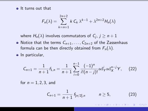
It turns out that

Fn(λ) =2n+2∑k=n+1

k Ck λk−1 + λ2n+2Hn(λ)

where Hn(λ) involves commutators of Cj , j ≥ n + 1

Notice that the terms Cn+1, . . . ,C2n+2 of the Zassenhausformula can be then directly obtained from Fn(λ).

In particular,

Cn+1 =1

n + 1f1,n =

1

n + 1

n−1∑i=0

(−1)n

i !(n − j)!adiY ad

n−jX Y , (22)

for n = 1, 2, 3, and

Cn+1 =1

n + 1f[n/2],n n ≥ 5, (23)

Algorithm

Define f1,k =k∑

j=1

(−1)k

j!(k − j)!adk−jY adjXY

C2 = (1/2) f1,1Define fn,k n ≥ 2, k ≥ n by :

fn,k =

[k/n]−1∑j=0

(−1)j

j!adjCn

fn−1,k−nj

Cn = (1/n)f[(n−1)/2],n−1 n ≥ 3.

(24)

Important property: it provides expressions for Cn that, byconstruction, involve only independent commutators. In otherwords, they cannot be simplified further by using the Jacobiidentity and the antisymmetry property of the commutator.

This can be easily proved by repeated application of theLazard elimination principle.

Computational aspects

The algorithm can be easily implemented in a symbolicalgebra package. We need to define an object inheriting onlythe linearity property of the commutator, the adjoint operatorand the functions fn,k and Cn.

We have expressions of Cn up to n = 20 with a reasonablecomputational time and memory requirements (35 MB).

n CPU time (seconds) Memory (MB)

W-S New W-S New

14 29.18 0.14 122.90 0.8816 203.85 0.59 764.32 4.0918 3.01 11.1220 19.18 35.27

C16 has 54146 terms when expressed as combinations ofwords, but only 3711 terms with the new formulation

Algorithm

Convergence

Suppose now that X and Y are defined in a Banach algebra AThen it makes sense to analyze the convergence of theZassenhaus formula.

Only two previous results establishing sufficient conditions forconvergence of the form ‖X‖+ ‖Y ‖ < r with a given r > 0.

Suzuki (1976): rs = log 2− 12 ≈ 0.1931

Bayen (1979): rb given by the unique positive solution of theequation

z2

(1 + 2

∫ z

0

e2w − 1

wdw

)= 4(2 log 2− 1).

Numerically, rb = 0.59670569 . . ..

Thus, for ‖X‖+ ‖Y ‖ < rb one has

limn→∞

eX eY eC2 · · · eCn = eX+Y . (25)

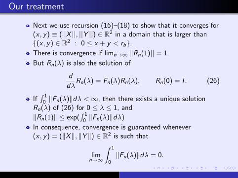
Our treatment

Next we use recursion (16)–(18) to show that it converges for(x , y) ≡ (||X ||, ||Y ||) ∈ R2 in a domain that is larger than(x , y) ∈ R2 : 0 ≤ x + y < rb.There is convergence if limn→∞ ||Rn(1)|| = 1.

But Rn(λ) is also the solution of

d

dλRn(λ) = Fn(λ)Rn(λ), Rn(0) = I . (26)

If∫ 1

0 ‖Fn(λ)‖dλ <∞, then there exists a unique solutionRn(λ) of (26) for 0 ≤ λ ≤ 1, and

‖Rn(1)‖ ≤ exp(∫ 1

0 ‖Fn(λ)‖dλ)

In consequence, convergence is guaranteed whenever(x , y) = (‖X‖, ‖Y ‖) ∈ R2 is such that

limn→∞

∫ 1

0‖Fn(λ)‖dλ = 0.

We have that ‖Cn+1‖ ≤ δn+1, where δ2 = x y and for n ≥ 2,

δn+1 =1

n + 1

∑(i0,i1,...,in)∈In

2i0+···+in

i0!i1! · · · in!δinn · · · δ

i22 y

i1x i0y .

Similarly, ‖Fn(λ)‖ ≤ fn(λ) and∫ 1

0fn(λ)dλ ≤

∞∑k=n

δk ,

Then, limn→∞ ||Rn(1)|| = 1 if the series∑∞

k=2 δk converges.

Let’s analyze each term in this series...

We get from our recurrence

‖f1,k‖ ≤ d1,k ≡ 2kyk∑

j=1

1

j!(k − j)!x jyk−j =

2k

k!y((x + y)k − yk

)‖fn,k‖ ≤ dn,k =

[k/n]−1∑j=0

2j

j!δjndn−1,k−nj (27)

Therefore

‖Cn‖ ≤ δn =1

nd[(n−1)/2],n−1, n ≥ 3.

A sufficient condition for convergence is obtained by imposing

limn→∞

δn+1

δn< 1. (28)

Recall that both dn,k and δn depend on (x , y) = (‖X‖, ‖Y ‖),so condition (28) implies a constraint on the convergencedomain (x , y) ∈ R2

Convergence domain

Computing numerically for each point the coefficients dn,k and δnup to n = 1000 we get

0.0 0.5 1.0 1.5 2.0 2.5 3.00.0

0.5

1.0

1.5

2.0

2.5

3.0

ÈÈXÈÈ

ÈÈY

ÈÈ

Example

X = α

(1 10 1

)and Y =

(1 01 0

)Compute R1 = e−Y e−X eX+Y

Compute R2(m) = eC2eC3 · · · eCm

Finally Em = ‖R1 − R2(m)‖Particular case: α = 0.2. Then we are outside the guaranteeddomain of convergence

m = 10, E10 ≈ 1.3345 · 10−4

m = 15, E15 ≈ 1.9180 · 10−6

m = 20, E20 ≈ 4.7958 · 10−9

Generalization

Sometimes one has to deal with

exp(λA1 + λ2A2 + · · ·+ λnAn + · · · )

with Ak non-commuting operators

In that case it is still possible to generalize the expansion andto get

eλA1+λ2A2+··· = eλC1eλ2C2 · · · eλnCn · · ·

Recursive procedure to obtain Ck

IV. MAGNUS EXPANSION

General linear differential equation

Goal

Given the matrix A(t) N × N, solve the initial value problem

Y ′(t) = A(t)Y (t), Y (t0) = Y0. (29)

If N = 1, the solution reads

Y (t) = exp

(∫ t

t0

A(s)ds

)Y0. (30)

This is also valid when N > 1 if [A(t),∫ t

0 A(s)ds] = 0.Particular case: A(t1)A(t2) = A(t2)A(t1) for all t1 y t2. Inparticular, when A is constant.

In general, (30) is not the solution

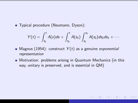
Typical procedure (Neumann, Dyson):

Y (t) =

∫ t

t0

A(s)ds +

∫ t

t0

A(s1)

∫ s1

t0

A(s2)ds2ds1 + · · ·

Magnus (1954): construct Y (t) as a genuine exponentialrepresentation

Motivation: problems arising in Quantum Mechanics (in thisway, unitary is preserved, and is essential in QM)

Magnus expansion

W. Magnus proposal: to express the solution as theexponential of a certain matrix function Ω(t, t0),

Y (t) = exp Ω(t, t0)Y0 (31)

Ω is built as a series expansion

Ω(t) =∞∑k=1

Ωk(t). (32)

For simplicity, Ω(t) ≡ Ω(t, t0) y t0 = 0.

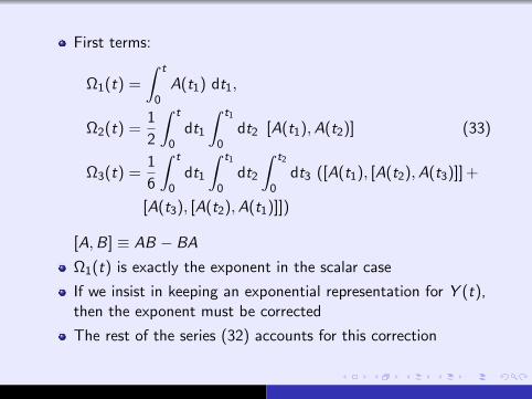
First terms:

Ω1(t) =

∫ t

0A(t1) dt1,

Ω2(t) =1

2

∫ t

0dt1

∫ t1

0dt2 [A(t1),A(t2)] (33)

Ω3(t) =1

6

∫ t

0dt1

∫ t1

0dt2

∫ t2

0dt3 ([A(t1), [A(t2),A(t3)]] +

[A(t3), [A(t2),A(t1)]])

[A,B] ≡ AB − BA

Ω1(t) is exactly the exponent in the scalar case

If we insist in keeping an exponential representation for Y (t),then the exponent must be corrected

The rest of the series (32) accounts for this correction

How the series is obtained?

Insert Y (t) = exp Ω(t) in Y ′ = A(t)Y , Y (0) = I

Differential equation satisfied by Ω:

dΩ

dt=∞∑n=0

Bn

n!adnΩA, (34)

where ad0ΩA = A, adk+1

Ω A = [Ω, adkΩA],and Bj are the Bernoulli number.

At first sight, a very bad idea!: we replace a linear differentialequation by another which is highly nonlinear!

... But this is defined for Ω

We apply Picard’s iteration:

Ω[0] = O, Ω[1] =

∫ t

0A(t1)dt1,

Ω[n] =

∫ t

0

(A(t1)dt1 −

1

2[Ω[n−1],A] +

1

12[Ω[n−1], [Ω[n−1],A]] + · · ·

)dt1

so that limn→∞Ω[n](t) = Ω(t) in a neighborhood of t = 0

Another recursive procedure to obtain the series, based on agenerator

When the recursion is worked out explicitly,

Ωn(t) =n−1∑j=1

Bj

j!

∑k1+···+kj=n−1

k1≥1,...,kj≥1

∫ t

0adΩk1

(s) adΩk2(s) · · · adΩkj

(s)A(s) ds n ≥ 2,

Ωn is a linear combination of n-multiple integrals ofn − 1-nested commutators containing n operators A evaluatedat different times

The expression is increasingly complicated when n grows

Some properties

If A(t) belongs to some Lie algebra g, then Ω(t) (andtruncation of the Magnus series) also belongs to g andtherefore exp(Ω) ∈ G, where G is the Lie group with Liealgebra g.

1 Symplectic group (in Hamiltonian mechanics)2 Unitary group (for the Schrodinger equation)

The resulting approximations preserve important qualitativeproperties of the exact solution (e.g., unitarity, etc.)

Analytic approximations

Starting point for the construction of new families ofnumerical integrators for Y ′ = A(t)Y

Very efficient high order numerical methods

Lie group integrators, special class of geometric numericalintegration methods

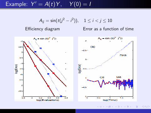
Example: Y ′ = A(t)Y , Y (0) = I

Aij = sin(t(j2 − i2)), 1 ≤ i < j ≤ 10

Efficiency diagram Error as a function of time

Convergence

Is this result only formal? What about convergence?

Specifically, given a certain operator A(t), when it is possibleto get Ω(t) in (31) as the sum of the seriesΩ(t) =

∑∞n=1 Ωn(t)?

It turns out that the Magnus series converges for t ∈ [0,T )such that ∫ T

0‖A(s)‖ds < π

where ‖ · ‖ is the 2-norm

This is a generic result, in the sense that it is possible to findparticular matrices A(t) so that the series diverges for allt > T .

... But is is only a sufficient condition: there exist matricesA(t) so that the expansion converges for t > T .

Analysis of the eigenvalues

Convergence

Remarks

The result is valid for complex matrices A(t)

In fact, for any given bounded operator A(t) in a Hilbert spaceH if Y is a normal operator (in particular, if iY is unitary).

This results can be used in turn to prove the convergence ofthe Baker–Campbell–Hausdorff formula

BCH and the Magnus expansion

Consider the initial value problem

U ′ = A(t)U, U(0) = I , (35)

with

A(t) =

Y 0 ≤ t ≤ 1X 1 < t ≤ 2

The exact solution of (35) at t = 2 is U(2) = eX eY .

But we can apply Magnus: U(2) = eΩ(2).

In this way it is possible to get BCH as a particular case of theMagnus expansion. (Sometimes it is called the continuousBCH formula BCH).

Work in progress

‘Symmetric’ Zassenhaus formula: useful for obtaining newnumerical methods for certain classes of PDEs (Bader et al.2014)

eX+Y = · · · eC3 eC2 e12Y eX e

12Y eC2 eC3 · · ·

in an efficient way

‘Continuous analogue’ of the Zassenhaus formula (M.Nadinic’s Thesis 2015): Given U ′ = A(t)Y , U(0) = I ,

U(t) = eW1(t) eW2(t) · · · eWr (t) · · ·

as efficiently as possible

Some references

S. Blanes, F.C., J.A. Oteo, J. Ros, The Magnus expansionand some of its applications, Physics Reports 470 (2009),151-238.S. Blanes and F.C., On the convergence and optimization ofthe Baker–Campbell–Hausdorff formula, Lin. Alg. Appl. 378(2004), 135-158.A. Bonfiglioli and R. Fulci, Topics in NoncommutativeAlgebra, Lecture Notes in Mathematics 2034. Springer, 2012.F.C. and A. Murua, An efficient algorithm for computing theBaker–Campbell–Hausdorff series and some of its applications.J. Math. Phys. 50 (2009), 033513.F.C., A. Murua and M. Nadinic, Efficient computation of theZassenhaus formula, Comput. Phys. Comm. 183 (2012),2386-2391.W. Magnus, On the exponential solution of differentialequations for a linear operator. Commun. Pure Appl. Math.VII (1954), 649-673.W. Magnus, A. Karrass and D. Solitar, Combinatorial GroupTheory. Dover, 2004.C. Reutenauer, Free Lie Algebras. Oxford University Press,1993.