Embed Size (px)
Citation preview

On Some Connections between
Nonlinear Filtering, Information Theory
and Statistical Mechanics
Sanjoy K. Mitter
Laboratory for Information and Decision SystemsMassachusetts Institute of Technology
Cambridge, MA, USA

Abstract
1. Some basic concepts in Probability Theory and Information Theory
2. Filtering, Control and Thermodynamics
Interaction of Communication and Control
3. Stochastic Linear Dynamical Systems. Kalman Filtering from the
Innovations viewpoint.
Separation Theorem
4. Dissipative Systems (J.C. Willems). Kalman Filter as an Informally
Dissipative System. Information Optimality of the Kalman Filter.
Nonlinear Generalization
5. Introduction to Statistical Mechanics. The Ising Model. Variational
Description of Gibbs Measures. Bayesian Inference as Free Energy
Minimization. The Duality between Estimation and Control

Introduction
• Problems of Control where Sensors, Actuators and Controllers are
linked via Noisy, Communication Channels
• Information Theory
• Stochastic Control with Partial Observations (Dynamics
Programming)
• Fundamental Limitations: Noisy Channel Coding Theorem
• LQG: Irreducible error
• Stablilization

• Energy Harvesting
• Recover Energy from Vibrating Motion
• Monitoring and Sensor Networks
• Integration of Physics, Information, Control and Computation

Dissipative Dynamical System (Willems)
: Dynamical Systems
(Soln. of state space system with read out map)
w(t) = w(u(t), y(t)) , integrable Supply rate
Definition:
A dynamical system with supply rate w is said to be
dissipative if ∀ nonnegative function S : X → R†, called the
“storage function” such that ∀ (t1, t0) ∈ R†2, x0 ∈ X and
u ∈ U
S(x0) +∫ t1
t0w(t)dt ≥ S(x1)
where x1 = ϕ(t1, t0;x0, u) and w(t) = w(u(t), y(t)) and
y = y(t0, x0, u).
1

Maximum Work Extraction and
Implementation Costs for
Non-equilibrium Maxwell’s Demons
by H. Sandberg, J.-C. Delvenne,
N.J. Newton and S.K. Mitter
in Physical Review E 90 042119 (2014)
2

Maximum work extraction and implementation
costs for non-equilibrium Maxwell’s demons
Ever since Maxwell [1] put forward the idea of an
abstract being (a demon) apparently able to
break the second law of thermodynamics, it has
served as a great source of inspiration and
helped to establish important connections
between statistical physics and information
theory [2–6]. In the original version, the demon
operates a trapdoor between two heat baths,
such that a seemingly counterintuitive heat flow
is established.3

Today, more generally, devices that are able to
extract work from a single heat bath by
rectifying thermal fluctuations are also called
“Maxwell’s demons” [7]. Several schemes
detailing how the demon could apparently break
the second law have been proposed, for example
Szilard’s heat engine [2]. More recent schemes
are presented in Refs. [7–12], where
measurement errors are also accounted for.
4

A classical expression of the second law states
the following: Maximum (average) work
extractable from a system in contact with a
single thermal bath cannot exceed the free
energy decrease between the system’s initial and
final equilibrium states.
However, as illustrated by Szilard’s heat engine,
it is possible to break this bound under the
assumption of additional information available to
the work-extracting agent.
Free Energy = Average Energy − Entropy5

To account for this possibility, the second law
can be generalized to include transformations
using feedback control [8,13–19]. In particular,
in Ref. [18] it is shown that under feedback
control, the extracted work W must satisfy
W ≤ kTIc, (1)
where k is Boltzmann’s constant, T is the
temperature of the bath, and Ic is the so called
transfer entropy from the system to the
measurement.
6

Note that in (1) we have assumed there is no
free energy decrease from the initial to the final
state. Related generalizations of the second law
are stated in Refs. [20–22]. It is possible to
construct feedback protocols that saturate (1)
using reversible and quasistatic transformations
[18,23,24]. Reversible feedback protocols may be
optimal in terms of making (1) tight, but they
are also infinitely slow, and in Refs. [17,25–29]
some related finite-time problems are addressed.
7

Our new contribution is to state an explicit
finite-time counterpart to (1), characterizing the
maximum work extractable using feedback
control, in terms of the transfer entropy.
To explain our result, consider a system modeled
by an overdamped Langevin equation. We show
that the maximum amount of extractable work
over a duration t, Wmax(t), can be expressed by
the integral
Wmax(t) = k∫ t
0TminIc dt
′ ≤ kTIc(t). (2)
8
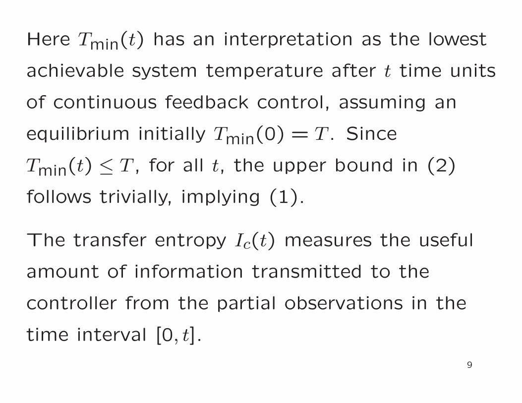
Here Tmin(t) has an interpretation as the lowest
achievable system temperature after t time units
of continuous feedback control, assuming an
equilibrium initially Tmin(0) = T . Since
Tmin(t) ≤ T , for all t, the upper bound in (2)
follows trivially, implying (1).
The transfer entropy Ic(t) measures the useful
amount of information transmitted to the
controller from the partial observations in the
time interval [0, t].
9
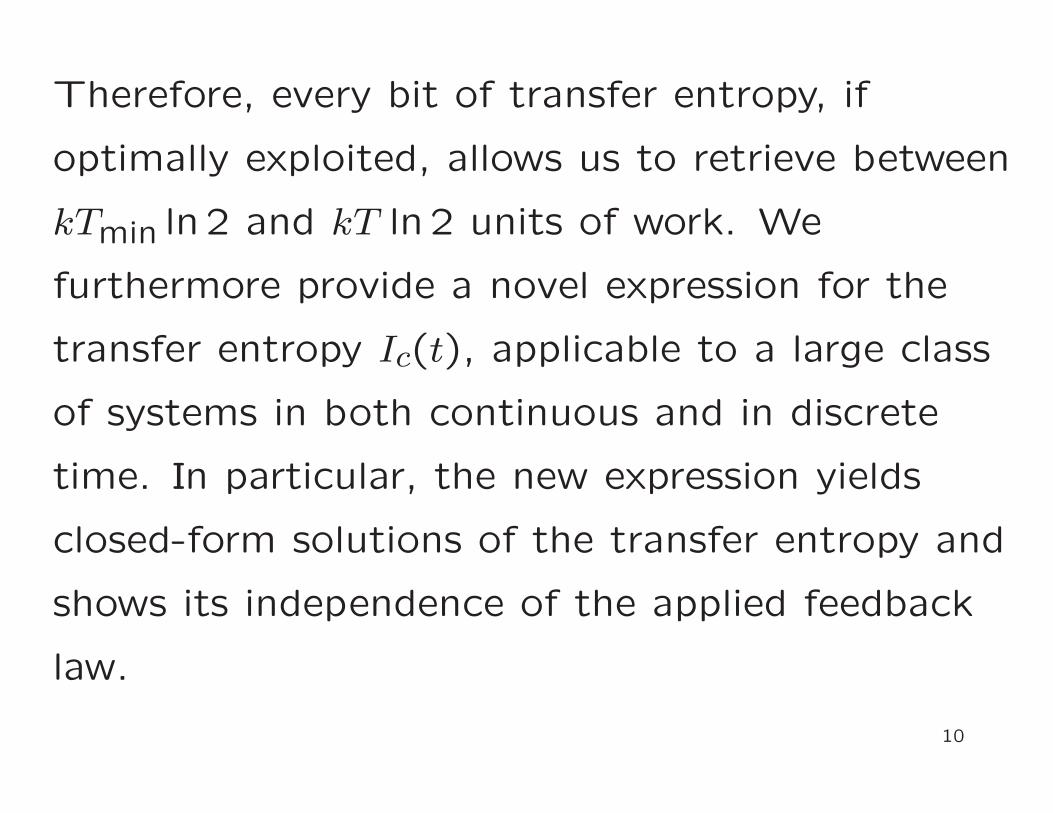
Therefore, every bit of transfer entropy, if
optimally exploited, allows us to retrieve between
kTmin ln 2 and kT ln 2 units of work. We
furthermore provide a novel expression for the
transfer entropy Ic(t), applicable to a large class
of systems in both continuous and in discrete
time. In particular, the new expression yields
closed-form solutions of the transfer entropy and
shows its independence of the applied feedback
law.
10

Our other contribution is to use control theory
to characterize and interpret the feedback
protocol the demon should apply to reach the
upper limit Wmax(t).
The protocol is a linear feedback law based on
the optimal estimate of the system state, which
can be recursively computed using the so-called
Kalman–Bucy filter. The found feedback law
also offers a simple electrical implementation.
11

A proper physical implementation is also shown
to require an external work supply to maintain
the noise on the wires at an acceptable level.
The cost of this noise suppressing mechanism
can be evaluated by standard thermodynamic
arguments, or through a non-equilibrium
extension of Landauer’s memory erasure
principle.
12
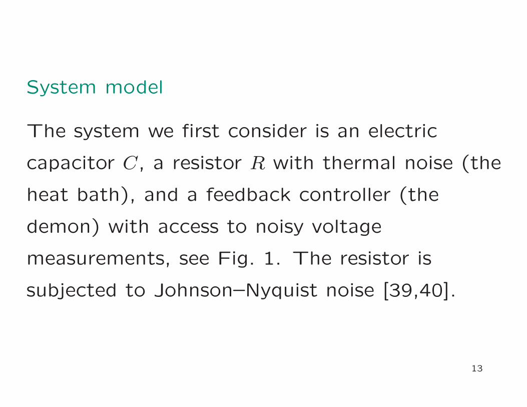
System model
The system we first consider is an electric
capacitor C, a resistor R with thermal noise (the
heat bath), and a feedback controller (the
demon) with access to noisy voltage
measurements, see Fig. 1. The resistor is
subjected to Johnson–Nyquist noise [39,40].
13

Demon
−+
2kT
RwRC
+
−
+
−
v
i
Vmeaswmeas
vmeas
FIG.1: The demon (the feedback controller) connected to
a capacitor, a heat bath of temperature T , and a
measurement noise source of intensity Vmeas. The demon
may choose the current i freely, and has access to the
noisy voltage measurement vmeas.
14

The circuit is modeled by an overdamped
Langevin equation
τ v = −v+Ri+√2kTRw, 〈v(0)〉 = 0,
vmeas = v+√Vmeaswmeas, 〈v(0)2〉 = kT
C,
(3)
with v(0) Gaussian, w and wmeas uncorrelated
Gaussian white noise (〈w(t)w(t′)〉 =〈wmeas(t)wmeas(t′)〉 = δ(t− t′)), Vmeas the
intensity of the measurement noise, and τ = RC
being the time constant of the open circuit.
15

The measurement noise√Vmeaswmeas can be
thought of as the Johnson–Nyquist noise of the
wire between the capacitor and the demon,
whose resistance for simplicity is incorporated in
the demon. The heat flow to the capacitor is Q
and the work-extraction rate of the demon is W ,
and satisfy the first law of thermodynamics,
U = Q− W (4)
where
16

U = 12C〈v2〉 ≡ 1
2kTC,
Q = kτ(T − TC), W = −〈vi〉.
(5)
We denote the effective instantaneous
temperature (“kinetic temperature”) of the
capacitor by TC, and its internal energy by U .
For detailed derivations of (4)–(5), see Ref. [37].
Furthermore, we assume the capacitor initially is
in thermal equilibrium with the heat bath, i.e.,
TC(0) = T .17

Just as in Ref. [17], we can justify calling TC(t) a
temperature since it appears in a Fourier-like
heat conduction law (see Q). Also, since our
applied controls will maintain a Gaussian
distribution of v, TC(t) will be the true
temperature of the capacitor if it were to be
disconnected from all the other elements at time
t. The voltage vmeas is the measurement that
supplies the demon with information, and can be
seen as a noisy measurement of the fluctuating
capacitor voltage v.18

We will show how a demon can optimally control
the work extraction by carefully exploiting the
measurements vmeas and properly choosing the
injected current i. Intuitively, the demon can
create a positive work rate W if it chooses i < 0
when it correctly estimates v > 0, and vice versa.
But how the demon should estimate v, and how
to optimally choose i may be less obvious.
19

If we know the trajectory of the effective
temperature TC, it is from (4) and (5) possible
to solve for the amount of extracted work,
W (t) =∫ t
0
k
τ(T − TC) dt
′ +1
2k(T − TC(t)). (6)
20

In particular, if we can characterize a lower
bound on the effective temperature under all
allowed controls, Tmin(t′) ≤ TC(t
′) for 0 ≤ t′ ≤ t,
we get an upper bound on the work that a
demon can extract,
Wmax(t) :=∫ t
0
k
τ(T − Tmin) dt
′ +1
2k(T − Tmin(t)),
(7)
so that W (t) ≤Wmax(t). In the following, we
characterize Tmin, and thereby Wmax, using
optimal control theory.
21

Demon model and optimal continuous-time
feedback
Optimal control theory [41] teaches how to
compute Tmin, and to characterize the
corresponding feedback law. In particular, for
linear systems the separation principle [42] says
we can achieve the goal in two steps: First, we
should continuously and optimally estimate the
voltage v(t) of the capacitance, given the
available measurements
(vmeas)t0 ≡ vmeas(t′), 0 ≤ t′ ≤ t.22

Second, we should continuously use the found
optimal estimate to update the current i(t) using
a suitable linear feedback law.
The best possible estimate v(t) of v(t), given the
measurement trajectory (vmeas)t0, can be
recursively constructed by the celebrated
Kalman–Bucy filter [43], which leads to a
minimum variance estimation error [41] and
exploits as much of the information contained in
vmeas as is possible [44].23

We give a brief background to the Kalman–Bucy
filter and its properties next. The filter state is
denoted v and satisfies the differential equation
τd
dtv = −v+Ri+K(vmeas − v), v(0) = 0, (8)
where K is a time-varying function to be
specified.
24

Guided by optimal control theory and the
separation principle, we let the demon use the
simple linear causal feedback
i(t′) = −Gv(t′), 0 ≤ t′ ≤ t, (9)
where 0 ≤ G <∞ is a fixed scalar feedback gain.
We may think of the feedback gain G as the
“conductance” of the demon: If the demon
believes the voltage of the capacitor to be v, it
will admit the current Gv. If v ≈ v, the demon
will indeed look like an electric load of
conductance close to G.25

While G = 0 (open circuit) creates a demon that
only (optimally) observes, G → ∞ also removes
energy from the capacitance at the highest
possible rate, achieving the minimum effective
temperature Tmin. This can be seen as follows:
Inserting (9) in (8) we can compute the evolution
of the variance V ≡ 〈v2〉 of the filter estimate as
τd
dtV = −2 (1+GR) V +
σkT2min
2CT, V (0) = 0.
(10)
26

We note that since Tmin is bounded, V can be
made arbitrarily close to zero by increasing the
feedback gain G. From (paper14) and
(paper15), it follows that
kTC
C= 〈v2〉 = 〈v2〉+ 〈∆v2〉 = V +
kTmin
C. (11)
Since Tmin is independent of G, and V can be
made arbitrarily close to zero, we realize that the
demon through its policy is cooling the capacitor
and for all t,
TC(t) ց Tmin(t) as G→ ∞. (12)
27

This shows a demon should implement a
Kalman–Bucy filter with a large (infinite)
feedback gain G to extract the work Wmax.
For a general feedback gain G ≥ 0 in (9), the
effective temperature of the capacitor will drop
exponentially from TC(0) = T to
TNESSC =
1
1+GRT +
GR
1+GRTNESSmin . (13)
28

The corresponding NESS work-extraction rate
can be shown to become
WNESS =k
τ(T − TNESS
min )GR
1+GR. (14)
Thus the continuous feedback protocol in (9)
can realize any NESS work rate between 0 and
the maximum WNESSmax = k
τ(T − TNESS
min ) by proper
choice of gain G.
The above optimal controller can be generalized
to any system with linear dynamics.29

Information flow and maximum work theorem
To establish the maximum work theorem in (2),
we need to quantify the information flow from
the uncertain part of the voltage v to the
measurement vmeas, under continuous feedback.
This is the transfer entropy, as is explained in
Ref. [18], for example.
30

We show that the appropriate continuous-time
limit of the transfer entropy is
Ic(t) = I((v(0), (w)t0); (vmeas)t0). (15)
This is the mutual information between the
uncertain initial voltage v(0) and noise trajectory
w from the bath, and the measurement
trajectory vmeas.
31

Mutual information [47] between two stochastic
variables ξ and θ is as usual defined as
I(θ; ξ) ≡∫
ln
dPθξ
d(Pθ ⊗ Pξ)
dPθξ ≥ 0, (16)
and is equal to the amount the (differential)
Shannon entropy of ξ decreases with knowledge
of θ, and vice versa.
32

Here Pθξ, Pθ, and Pξ are joint and marginal
probability measures of the stochastic variables θ
and ξ. We prove that the transfer entropy in fact
has the following explicit form:
Ic(t) =σ
4τ
∫ t
0
Tmin
Tdt′. (17)
Note that Ic does not otherwise depend on the
details of the demon, for example the feedback
gain G.
33

It now follows from Eqs. (7), (paper11), and
(17) that the maximum extracted work must
satisfy
Wmax(t) =∫ t
0
k
τ(T − Tmin) dt
′ +1
2k(T − Tmin(t))
=∫ t
0
σkT2min
4τTdt′ = k
∫ t
0TminIc dt
′, (18)
which proves the equality in (2). The inequality
trivially follows since Tmin ≤ T .
34

The expressions for Ic and Wmax provide
interesting insights concerning information and
work flow in the feedback loop. Since Tmin
decreases monotonically, the transfer entropy
rate Ic is largest just when the measurement and
feedback control start, and then decreases until
it stabilizes at
INESSc =
σTNESSmin
4τT=
√1+ σ − 1
2τ. (19)
35

In NESS, the fresh measurements are no longer
able to improve the quality of the estimate, i.e.,
to decrease the error variance 〈[v(t)− v(t)]2〉 any
further. Since Wmax = kTminIc, the
work-extraction rate also decreases until it
stabilizes at
WNESS = kTminINESSc
GR
1+GR, (20)
see (14).
36

As in related studies [18,23,26], we can now
define and study the information efficiency η of
the demon,
η ≡ W
kTIc∈ [0,1]. (21)
It measures the amount of extracted work per
unit of received useful information. An η ≈ 1
means that the demon is close to saturating (1),
and is operating at the limit of the generalized
second law of thermodynamics.
37

For our demons in NESS, we obtain the
efficiency
ηNESS =Tmin
T
GR
1+GR, (22)
using (20). Hence, only a maximum work demon
(G→ ∞) with Tmin ≈ T will operate at an
information efficiency close to 1. This
corresponds to the poor measurement limit
(σ ≈ 0), and a very small maximum work rate. A
demon with access to almost perfect
measurements (σ → ∞) has Tmin ≈ 0, and a very
low information efficiency, η ≈ 0.38
Note also that a less aggressive demon (small G)
has a lower efficiency, but that this is by choice:
The transfer entropy rate is independent on G,
and a smaller G decreases W , leading to a lower
efficiency.
39

REFERENCES
[1 ] Maxwell, J. C., Theory of Heat, (Longmans, London, 1871).
[2 ] Szilard, L. Z. Phys. 53, 840 (1929).
[3 ] Landauer, R., IBM Journal of Research and Development 5, 183
(1961).
[4 ] Bennett, C. H., International Journal of Theoretical Physics 21,
905 (1982).
[5 ] Penrose, O., Foundations of Statistical Mechanics: A Deductive
Treatment, Dover Books on Physics Series (Dover, London,
2005).
[6 ] Leff, H. and Rex, A., Maxwell’s Demon 2 Entropy, Classical and
Quantum Information, Computing, Maxwell’s Demon (CRC Press,
Boca Raton, 2010).
[7 ] D. Mandal, H. T. Quan, and C. Jarzynski, Phys. Rev. Lett. 111,
030602 (2013).
[8 ] J.M. Horowitz and S. Vaikuntanathan, Phys. Rev. E 82, 061120
(2010).
[9 ] T. Sagawa and M. Ueda, Phys. Rev. Lett. 109, 180602 (2012).
[10 ] P. Strasberg, G. Schaller, T. Brandes, and M. Esposito, Phys.
Rev. Lett. 110, 040601 (2013).
[11 ] D. Mandal and C. Jarzynski, PNAS 109, 11641 (2012).
[12 ] A. C. Barato andU. Seifert, Phys. Rev. Lett. 112, 090601
(2014).
[13 ] H. Touchette and S. Lloyd, Phys. Rev. Lett. 84, 1156 (2000).
[14 ] H. Touchette and S. Lloyd, Physica A 331, 140 (2004).
[15 ] T. Sagawa and M. Ueda, Phys. Rev. Lett. 104, 090602 (2010).

[16 ] Y. Fujitani and H. Suzuki, J. Phys. Soc. Jpn. 79, 104003 (2010).
[17 ] D. Abreu and U. Seifert, Europhys. Lett. 94, 10001 (2011).
[18 ] T. Sagawa and M. Ueda, Phys. Rev. E 85, 021104 (2012).
[19 ] S. Ito and T. Sagawa, Phys. Rev. Lett. 111, 180603 (2013).
[20 ] H.-H. Hasegawa, J. Ishikawa, K. Takara, and D. Driebe, Phys.
Lett. A 374, 1001 (2010).
[21 ] M. Esposito and C. V. den Broeck, Europhys. Lett. 95, 40004
(2011).
[22 ] S. Deffner and C. Jarzynski, Phys. Rev. X 3, 041003 (2013).
[23 ] J. M. Horowitz and J.M. R. Parrondo, Europhys. Lett. 95, 10005
(2011).
[24 ] J. M. Horowitz, T. Sagawa, and J. M. R. Parrondo, Phys. Rev.
Lett. 111, 010602 (2013).

[25 ] T. Schmiedl and U. Seifert, Phys. Rev. Lett. 98, 108301 (2007).
[26 ] M. Bauer, D. Abreu, and U. Seifert, J. Phys. A: Math. Theor.
45, 162001 (2012).
[27 ] G. Diana, G. B. Bagci, andM. Esposito, Phys. Rev. E 87,
012111 (2013).
[28 ] P. R. Zulkowski and M. R. DeWeese, Phys. Rev. E 89, 052140
(2014).
[29 ] M. Bauer, A. C. Barato, and U. Seifert, J. Stat. Mech. (2014)
P09010.
[37 ] J.-C. Delvenne and H. Sandberg, Physica D 267, 123 (2014).
[39 ] J. B. Johnson, Phys. Rev. 32, 97 (1928).
[40 ] H. Nyquist, Phys. Rev. 32, 110 (1928).

[41 ] K. J. A strom, Introduction to Stochastic Control Theory, Dover
Books on Electrical Engineering Series (Dover, London, 2006).
[42 ] W. Wonham, SIAM J. Control 6, 312 (1968).
[43 ] R. S. Bucy and P. D. Joseph, Filtering for Stochastic Processes
with Applications to Guidance (Interscience, New York, 1968).
[44 ] S. K. Mitter and N. J. Newton, J. Stat. Phys. 118, 145 (2005).

Towards a Unified View
of
Communication and Control
Sanjoy K. Mitter
Laboratory for Information and Decision Systems
Massachusetts Institute of Technology

INTRODUCTION
1. Partially observable stochastic control
problem
2. Feedback communication problem
3. Interaction of information and control
4. A general view of interconnection
5. Are communication problems really
different from control problems?
40

1. Partially Observable Stochastic Control
41

1. Partially observable stochastic control
1.1 Formulation
(1.1)Xn+1 = Fn(Xn, un, ξn) , n = 0,1,2, . . .
(1.2) Yn+1 = Gn(Xn, ηn) , n = 0,1,2, . . .
Hidden
Markov
Process
E = State space
U = Control space
E1 = Observation space
ξi ∈ S1 ; ηi ∈ S2
Assume: X0, (ξi), (ηi) are independent
Admissible strategy π := u0(y0), u1(y0, y1), . . .
sequence of measurable mappings
Cost function:
JN(π,X0) = E(N−1∑
n=0
qn(Xn, un) + rN(Xn))(1.3)
JN to be minimized by choice of π.
42
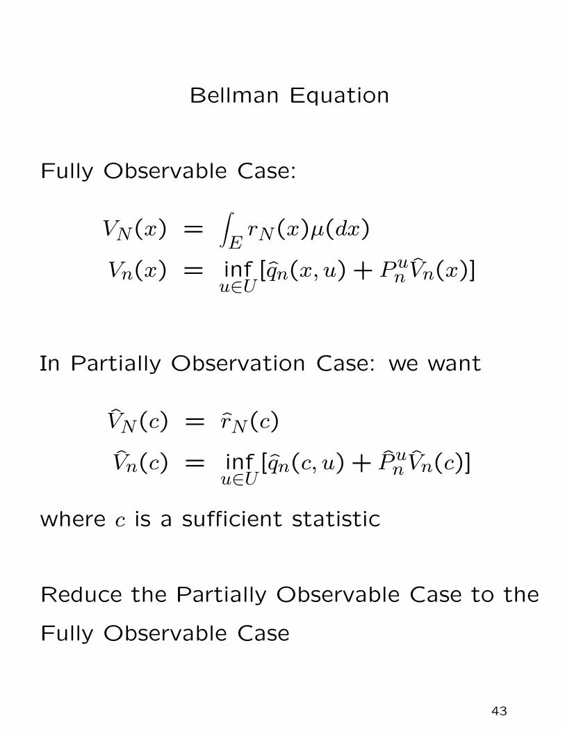
Bellman Equation
Fully Observable Case:
VN(x) =∫
ErN(x)µ(dx)
Vn(x) = infu∈U
[qn(x, u) + Pun Vn(x)]
In Partially Observation Case: we want
VN(c) = rN(c)
Vn(c) = infu∈U
[qn(c, u) + Pun Vn(c)]
where c is a sufficient statistic
Reduce the Partially Observable Case to the
Fully Observable Case
43
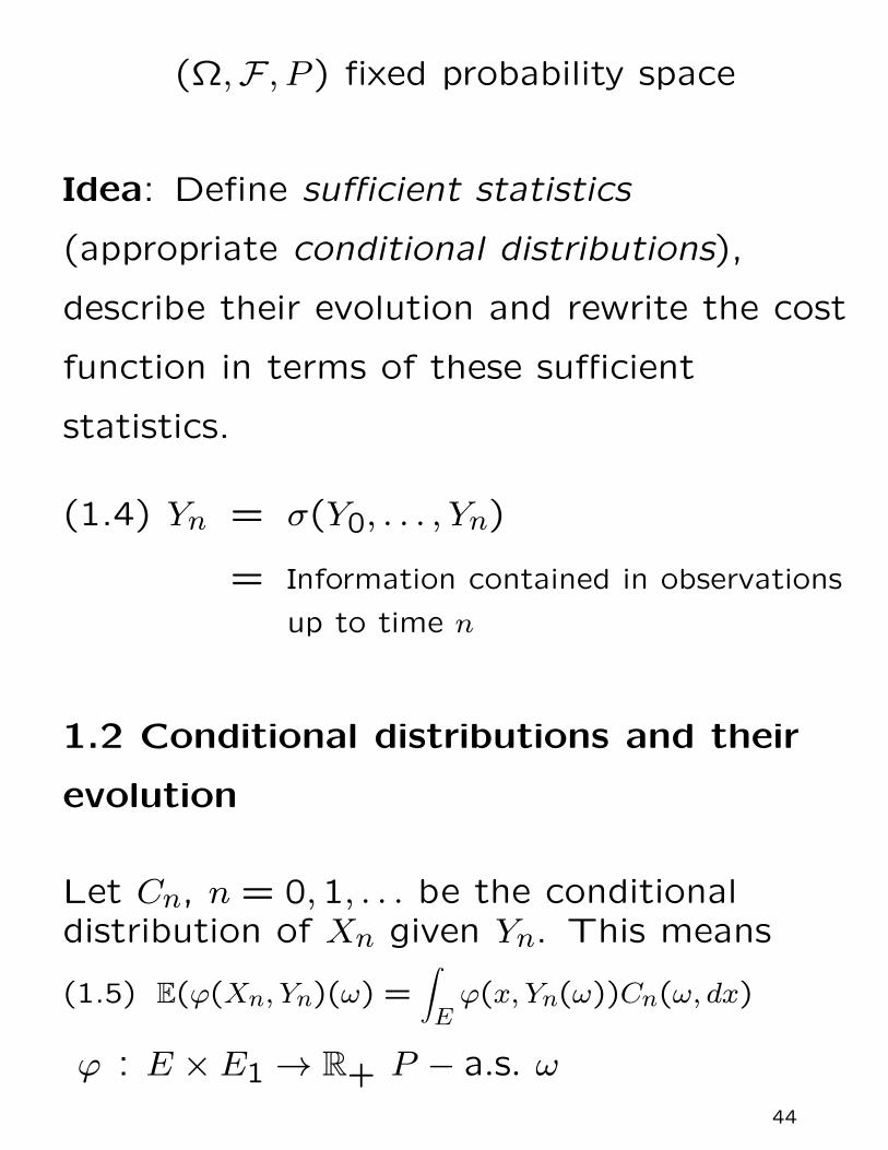
(Ω,F , P ) fixed probability space
Idea: Define sufficient statistics
(appropriate conditional distributions),
describe their evolution and rewrite the cost
function in terms of these sufficient
statistics.
Yn = σ(Y0, . . . , Yn)(1.4)
= Information contained in observations
up to time n
1.2 Conditional distributions and their
evolution
Let Cn, n = 0,1, . . . be the conditionaldistribution of Xn given Yn. This means
E(ϕ(Xn, Yn)(ω) =
∫
Eϕ(x, Yn(ω))Cn(ω, dx)(1.5)
ϕ : E ×E1 → R+ P − a.s. ω
44

Subtlety: The observations (Yn)n=0,1,...
depend on the control sequence
(un(y0, . . . , yn))n=0,1,... and, in turn, the
control sequence depends on the
observations.
It can be shown that the sequence(Cn)n=0,1,... of conditional distributions is aControlled Markov Chain with atime-dependent and control-dependenttransition function:
Punψ(c) =(1.6)
E
[∫
Eψ[Fn(c, u,Gn+1(Fn(x, u, ξn), ηn+1))]c(dx)
]
where E ⊂ P(E) measurable
Fn : E → R+
c ∈ E
ψ ∈ Bb(E)
45

Furthermore, in many situations, one can
show that there exists a sequence of
independent random variables (ξL)i=0,1,...
taking values in S1 (Innovations sequence)
and measurable mappings:
Fn : E × U × S1 → E s.t.
Cn+1 = Fn(Cn, un, ξn) , n = 0,1, . . .(1.7)
Note: Loop between control and
observation has been eliminated
Define:
qn(c, u) =∫
Eqn(x, u)c(dx) , n = 0,1, . . .(1.8)
rN(c) =
∫
ErN(x)c(dx) ,
c ∈ E
u ∈ U(1.9)
46

Bellman Equations
VN(c) = rN(c)(1.10)
Vn(c) = infu∈U
[qn(c, u) + Pun Vn(c)](1.11)
= qn(c, un(c)) + P unn Vn(c)
n = 0,1,2, . . .
Theorem: Optimal strategy π is
determined by the sequence:
u0(c0), u1(c1, c0), . . .
where c0, c1, . . . are functions of
y0, (y0, y1), . . . given recursively by
Cn+1 = Fn(cn, un(cn), yn+1)(1.12)
c0 = E(X0|Y0)
Min. Cost = E(V0(c0))(1.13)
47

Separation Theorem
Estimation and Control Separate
Average Cost Problem
min limN→∞
1
NE
N−1∑
n=0qn(xn, un) + rN(xN)
Minimization is over all strategiess
π := u0(y0), u1(y0, y1), . . .
48

Feedback Communication
Ref: S. Tatikonda and S.K. Mitter:
The Capacity of Channels with Feedback,
IEEE Trans. on Information Theory, Vol.
55, Jan. 2009, pp. 323–349.
49

2. Feedback Communication Problem
50

2. Feedback communication problem
Figure 1. Interconnection
Choose encoder and decoder to transmit message
over the channel to minimize the probability of error
Channel at time t: P(dbt|at, bt−1) stochastic kernel
at = (a0, . . . , at)
Channel = Sequence of P(dbt|at, bt−1)∣
∣
∣
t
t=1(2.1)
Time ordering: Message = W,A1, B1, , AT , BT , W =
Decoded message
W = (1,2, . . . ,M)
51

Code function:
Ft = ft : Bt−1 → A : measurable(2.2)
FT =T∏
t=1
Ft
Channel code function: fT = (f1, . . . , ft)
Distribution on code functions: P(dft|f t−1)∣
∣
∣
T
t=1
Channel code = list of M channel code functions
Code functions are introduced to reduce the
feedback communication problem to a no feedback
communication problem.
52

Average Measure of Dependence
Mutual Information
I(AT ;BT ) = EPAT ,BT
log
(
PAT ,BT
PATPBT
)
(2.3)
= EPAT ,BT
log
(
PBT |AT
PBT
)
I(AT ;BT ) =T∑
t=1
I(AT ;Bt|Bt−1)
Information transmitted to the receiver depends on
future (At+1, . . . , AT).
Directed Mutual Information (Causal)
I(AT → BT ) =T∑
t=1
I(At;Bt|Bt−1)(2.4)
53
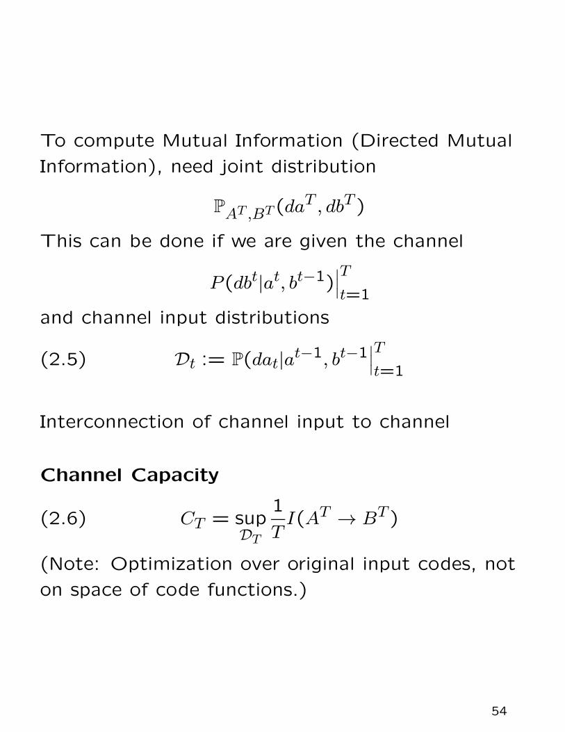
To compute Mutual Information (Directed Mutual
Information), need joint distribution
PAT ,BT (daT , dbT )
This can be done if we are given the channel
P(dbt|at, bt−1)∣
∣
∣
T
t=1
and channel input distributions
Dt := P(dat|at−1, bt−1∣
∣
∣
T
t=1(2.5)
Interconnection of channel input to channel
Channel Capacity
CT = supDT
1
TI(AT → BT )(2.6)
(Note: Optimization over original input codes, not
on space of code functions.)
54
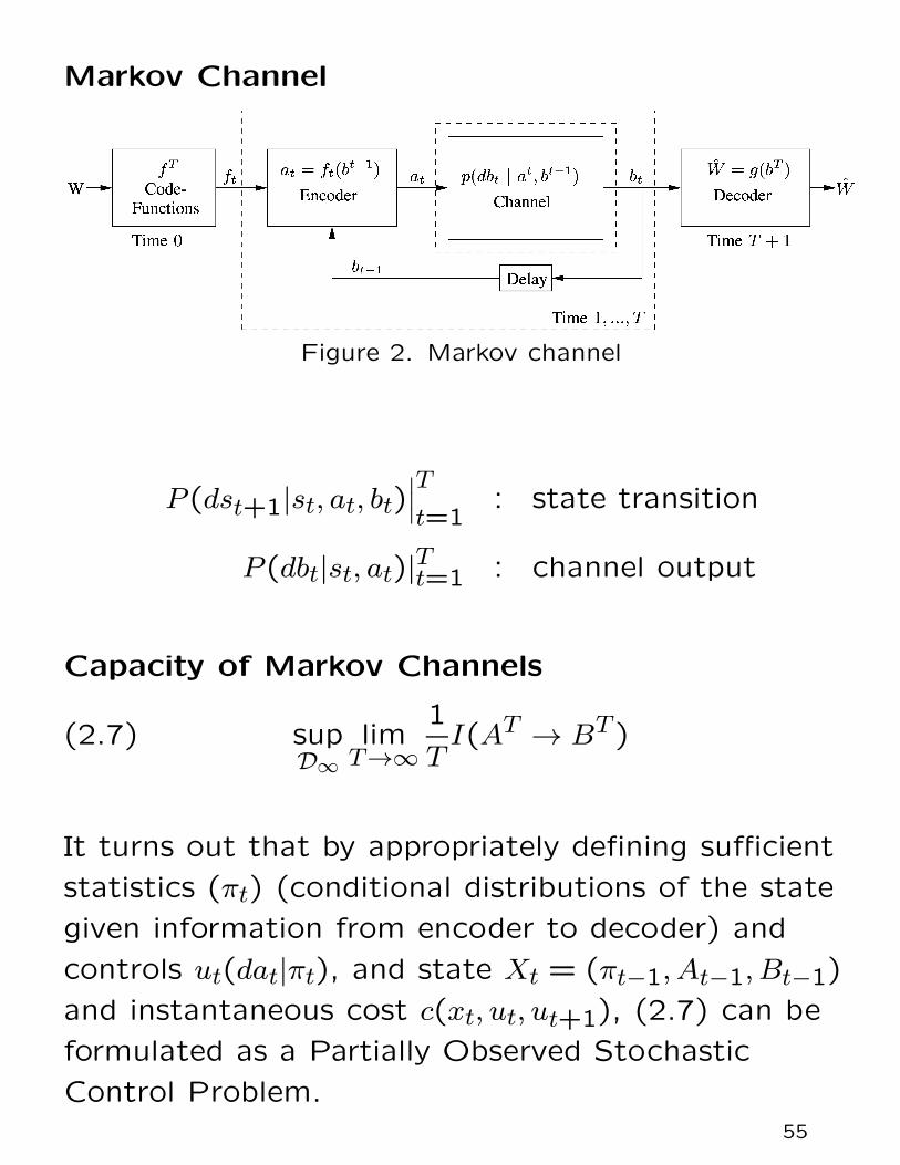
Markov Channel
Figure 2. Markov channel
P(dst+1|st, at, bt)∣
∣
∣
T
t=1: state transition
P(dbt|st, at)|Tt=1 : channel output
Capacity of Markov Channels
supD∞
limT→∞
1
TI(AT → BT )(2.7)
It turns out that by appropriately defining sufficient
statistics (πt) (conditional distributions of the state
given information from encoder to decoder) and
controls ut(dat|πt), and state Xt = (πt−1, At−1, Bt−1)
and instantaneous cost c(xt, ut, ut+1), (2.7) can be
formulated as a Partially Observed Stochastic
Control Problem.
55

In turn, as shown in Part 1, this can be reformulated
as a fully-observable stochastic control problem.
This problem is more like a dual control problem
since the choice of the channel input can help the
decoder identify the channel.
This is also an example where the information
pattern is nested: The encoder has more information
than the decoder.
56

The Interaction of Control and Communication
Sanjoy K. MitterMIT

!
"
#
$
Big questions about communication.
• Are all communication problems asymptotically alike?
• How does delay interact with capacity issues?
• Can we find examples that let us explore these questions in anasymptotic setting?
“. . . can be pursued further and is related to a dualitybetween past and future and the notions of control andknowledge. Thus we may have knowledge of the past andcannot control it; we may control the future but have noknowledge of it.” — Claude Shannon 1959
November 7, 2005 at UMD College Park

!
"
#
$
An abstract model of single channel problems
!"
#$
!"
"
#
!$
!
Source
Ut
Wt
Designed
DesignedSpecified
St
Encoder
Et
Feedback and Memory
Decoder
1 Step
Ut!1
Dt
ChannelNoisy
$ "
#
"
Xt
From Pattern I
delay
VtCommon Randomness R"1
Yt
Zt
fc
• Problem: Source S, Information pattern I, and Objective V.
• Constrained resource: Noisy channel fc
• Designed solution: “Encoder” E , “Decoder” D
November 7, 2005 at UMD College Park
!
"
#
$
Focus: what channels are “good enough”
• fc solves the problem if !E ,D so system satisfies V
• Problem A is harder than problem B if any fc that solves A
solves B.
• Information theory is an asymptotic theory
– Pick V family with an appropriate “slack” parameter
– Consider the set of channels that solve the problem.
– Take union over slack parameter choices.
November 7, 2005 at UMD College Park

!
"
#
$
The Shannon problems AR,!,d
• Source: noninteractive Xi (R bits): fair coin tosses
• Information pattern: Di has access to Zi1
– Af With feedback: Ei gets Xi1 and Zi!1
1
– Anf Without feedback: Ei gets only Xi1
• Performance objective: V(!, d) is satisfied if P(Xi "= Ui+d) # !
for every i $ 0.
– Slack parameter: permitted delay d
– Natural orderings: larger !, d is easier but larger R is harder.
• Classical capacity
CfR =
!
!>0
!
R#<R
"
d>0
fc|fc solves AfR#,!,d
CShannon(fc) = supR > 0|fc % CR
November 7, 2005 at UMD College Park

!
"
#
$
Classical relationships
• Feedback doesn’t change capacity for memoryless channels Cm
CnfR & Cm = Cf
R & Cm
• Zero-error capacity
Cf0,R =
!
R#<R
"
d>0
fc|fc solves AfR#,0,d
C0(fc) = supR > 0|fc % C0,R
– Can change with feedback even for memoryless channels
(Cnf0,R & Cm) ' (Cf
0,R & Cm)
– Zero-error problem is fundamentally harder
(Cnf0,R & Cm) ' (Cf
0,R & Cm) ' (CR & Cm)
November 7, 2005 at UMD College Park

!
"
#
$
Estimation with distortion: A(FX ,",D,d)
• Source: noninteractive Xi drawn iid from FX
• Same information patterns: with/without feedback.
• Performance objective: V(",D, d) is satisfied iflimn"#
1nE[
#ni=1 "(Xi, Ui+d)] # D.
– Slack parameter: permitted delay d
– Natural orderings: larger D, d is easier
• Channels that are good enough
Cfe,(FX ,",D) =
!
D#>D
"
d>0
fc|fc solves Af(FX ,",D#,d)
• “Separation Theorem” if " is finite.
(CR(D) & Cm) = (Cnfe,(FX ,",D) & Cm) = (Cf
e,(FX ,",D) & Cm)
November 7, 2005 at UMD College Park

!
"
#
$
Stabilization and anytime communication
• Simple control problem
• Why classical capacity.is not enough.
• Why anytime (delay-universality) is needed
• Some simple implications (power laws, etc.)
November 7, 2005 at UMD College Park

!
"
#
$
A simple scalar distributed control problem
1 StepDelay
%&
'(Channel
Noisy
DesignedObserver
DesignedController
%&
'(!
"
"
#
!
Possible Control Knowledge#
Possible Channel Feedback
1 StepDelay
#
$
Ut
Control Signals
O
C
Xt
Wt
Ut!1
ScalarSystem
$ "
Xt+1 = #Xt + Ut + Wt
• Unstable # > 1, bounded initial condition and disturbance W .
• Goal: Stability = supt>0 E[|Xt|#] # K for some K < (.
November 7, 2005 at UMD College Park

!
"
#
$
Is Shannon capacity all we need?
• Consider a system with
– # = 2 for the dynamics
– noisy channel that sometimes drops packets but is otherwisenoiseless (Real erasure channel)
Zt =
$%
&Yt with Probability 1
2
0 with Probability 12
• No other constraints, so design is obvious: Yt = Xt andUt = )#Zt
• Resulting closed loop dynamics:
Xt+1 =
$%
&Wt with Probability 1
2
2Xt + Wt with Probability 12
November 7, 2005 at UMD College Park

!
"
#
$
Is the closed-loop system stable?
Xt+1 =
$%
&Wt with Probability 1
2
2Xt + Wt with Probability 12
• i.i.d. erasures mean arbitrarily long stretches of erasures arepossible, though unlikely.
– System is not guaranteed to stay inside any box.
– Under stochastic disturbances, the variance of the state isasymptotically infinite.
• For worst case disturbances Wt = 1, the tail probability isdying o! as P (|X| > x) * K
x .
• Meanwhile, C = (!
November 7, 2005 at UMD College Park

!
"
#
$
Run same plant X over noiseless channel
Window known to contain Xt
Sending R bits, cut window by a factor of 2!R
0 1
"
!$
%%&
''(
"$! $!
grows by !2 on each side
giving a new window for Xt+1
will grow by factor of ! > 1
"t+1
Encode which control Ut to apply
!!t
"t
As long as R > log2 #, we can have " stay bounded forever.
November 7, 2005 at UMD College Park

!
"
#
$
What is needed: key intuition
• Break state X into sum of X (response to disturbance) and X
(response to control)
• Suppose # = 2 and so Xt =#t
i=0 2iWt!1
• Assume Wj either 0 or 1
• In binary notation: Xt = W0W1W2 . . .Wt!1.00000 . . .
• If )Xt is close to Xt, their binary representations likely agreein all the high-order bits.
– High-order bits represent earlier disturbances.
– Typically, to get a di!erence at the Wt!d level, we have tobe o! by about 2d.
Stabilization implies communicating bits reliably in aspecial fashion.
November 7, 2005 at UMD College Park

!
"
#
$
Anytime communication problems: AR,#,K
• Same as Shannon problem in source and information pattern.
• Performance objective di!erent:
– Reinterpret Ut = 0.X0(t), X1(t), X2(t), . . . in binary
– V(K,$) is satisfied if P(Xi "= Xi(i + d)) # K2!$d for everyi $ 0, d $ 0.
– Slack parameter: constant factor K
– Natural orderings: larger K is easier, but larger R,$ areharder.
• Capacity
Cfa,(R,$) =
!
R#<R
!
$#<$
"
K>0
fc|fc solves Af(R#,$#,K)
Cany(fc,$) = supR > 0|fc % Cfa,(R,$)
November 7, 2005 at UMD College Park

!
"
#
$
Separation theorem for control
Necessity: If a scalar system with parameter # > 1 can bestabilized with finite %-moment across a noisy channel, then thechannel with noiseless feedback must have
Cany(% log2 #) $ log2 #
In general: If P (|X| > m) < f(m), then !K : Perror(d) < f(K#d)
Su!ciency: If there is an $ > % log2 # for which the channel withnoiseless feedback has
Cany($) > log2 #
then the scalar system with parameter # $ 1 with a boundeddisturbance can be stabilized across the noisy channel with finite%-moment.
November 7, 2005 at UMD College Park

!
"
#
$
What does all this imply?
• If we want P (|Xt| > m) # f(m) = 0 for some finite m, werequire zero-error reliability across the channel.
• For generic DMCs, anytime reliability with feedback isupper-bounded:
f(K#d) $ &d
f(m) $ &log2( m
K)
log2 !
f(m) $ K $m!log2
1"
log2 !
A controlled state can have at best a power-law tail.
• If we just want limm"# f(m) = 0, then just Shannon capacity> log2 # is required for DMCs.
• Almost-sure stabilization for Wt = 0 follows by time-varyingtransformation.
November 7, 2005 at UMD College Park

!
"
#
$
Stabilization and Anytime Equivalence
• With nested information: Af%,#,K . Without: Anf
– Slack parameter: K (Performance)
– Natural ordering: larger %,# are harder, but larger K iseasier.
Cfs,(%,#) =
!
%#<%
!
##<#
"
K>0
fc|fc solves Af(%#,##,K)
• Equivalences
Cnfs,(%,#) + Cf
s,(%,#) = Cfa,(log2 %,# log2 %)
(Cnfs,(%,#)&C
finite) = (Cfs,(%,#)&C
finite) = (Cfa,(log2 %,# log2 %)&C
finite)
November 7, 2005 at UMD College Park

!
"
#
$
Asymptotic communication problem hierarchy
• The easiest: Shannon communication
– Asymptotically: a single figure of merit C
– Equivalent to most estimation problems of stationaryergodic processes with bounded distortion measures.
– Feedback does not matter.
• Intermediate families: Anytime communication
– Multiple figures of merit: ( 'R, '$)
– Feedback case equivalent to stabilization problems
– Related nonstationary estimation problems fall here also
– Does feedback matter?
• Hardest level: Zero-error communication
– Single figure of merit C0
– Feedback matters.
November 7, 2005 at UMD College Park

Language of Probability Theory
Probability Space
( ,F , P )
F = σ-field
= class of subsets of , closed under
complementation, countable
intersections, countable unions.
74

A nonnegative set function P ( · ) defined on F is
a Probability Measure if
(i) P ( ) = 1
(ii) ∀ finite, countable collection Bk of subsets
of F s.t.
Bk ∩Bj = φ , k 6= j
P (∩kBk) =
∑
kP (Bk)
75

Given ( ,F , P ) a Probability space
f : → R measurable
L2( ,F , P ) = f | ∫ |f |2dP <∞
Finite Energy signal
G ⊂ F, sub σ-field
L2( ,G, P )
E(F|G) = Projection of L2( ,F , P ) onto L2( ,G, P )
76

Conditional Expectation
“Nonlinear” Projection
(Xt)t≥0: Stochastic Process
E(Xt|Xs, s < t) = Xs a.s.
Martingale
77

Independence and Conditional Independence
σ-field generated by (Xt)t∈T = smallest σ-field
such that ∀ Xt are measurable
Markov Process
78

Past and Future Conditionally Independent given
the present
σ(Xs|s < t) ⊥ σ(Xs|s > t) | σ(Xt)Past Future Present
Why we need this language:
See J.C. Willems, “Open Stochastic Systems,”
IEEE Trans. on Automatic Control, 2013.
79

Wiener and Kalman Filtering
“Filtering and Stochastic Control:
A Historical Perspective”
by S.K. Mitter
in IEEE Control Systems
pp.67-76, June 1996

Wiener and Kalman Filtering
In order to introduce the main ideas of nonlinear
filtering, we first consider linear filtering theory.
A rather comprehensive survey of linear filtering
theory was undertaken by Kailath in [1] and
therefore we shall only expose those ideas which
generalize to the nonlinear situation.
80

Suppose we have a signal process (zt) and an
orthogonal increment process (wt), the noise
process and we have the observation equation
yt =∫ t
0zsds+ wt . (23)
Note that if (wt) is Brownian motion then this
represents the observation
y = zt+ ηt . (24)
where ηt is the formal (distributional) derivative
of Brownian motion and hence it is white noise.81

We make the following assumptions.
(A1) (wt) has stationary orthogonal increments
(A2) (zt) is a second-order q.m. continuous
process
(A3) For ∀s and t > s
(wt − ws) ⊥ Hw,zs
where Hw,zs is the Hilbert space spanned by
(wτ , zτ |τ ≤ s).82
The last assumption is a causality requirement
but includes situations where the signal zs may
be influenced by past observations as would
typically arise in feedback control problems. A
slightly stronger assumption is
(A3′) Hw ⊥ Hz
which states that the signal and noise are
uncorrelated, a situation which often arises in
communication problems.83

The situation which Wiener considered
corresponds to (24), where he assumed that (zt)
is a stationary, second-order, q.m. continuous
process.
84

The filtering problem is to obtain the best linear
estimate zt of zt based on the past observations
(ys|s ≤ t). There are two other problems of
interest, namely, prediction, when we are
interested in the best linear estimate z′r, r > t
based on observations (ys|s ≤ t) and smoothing,
where we require obtaining the best linear
estimate z′r, r < t based on observations (ys|s ≤ t).
85

Abstractly, the solution to the problem of
filtering corresponds to explicitly computing
zt = Pyt (zt) (25)
where Pyt is the projection operator onto the
Hilbert space Hyt . We proceed to outline the
solution using a method originally proposed by
Bode and Shannon [2] and later presented in
modern form by Kailath [3]. For a textbook
account see Davis [4] and Wong [5], which we
largely follow.86

Let us operate under the assumption (A3)′,
although all the results are true under the weaker
assumption (A3). The key to obtaining a
solution is the introduction of the innovations
process
νt = yt −∫ t
0zsds . (26)
87

The following facts about the innovations
process can be proved:
(F1) νt is an orthogonal increment process.
(F2) ∀s, ∀t > s
νt − νs ⊥ Hys and cov(νt) = cov(wt)
(F3) Hyt = Hν
t .
88

The name “innovations” originates in the fact
that the optimum filter extracts the maximal
probabilistic information from the observations in
the sense that what remains is essentially
equivalent to the noise present in the
observation. Furthermore, (F3) states that the
innovations process contains the same
information as the observations. This can be
proved by showing that the linear transformation
relating the observations and innovations is
causal and causally invertible.89

As we shall see later, these results are true in a
much more general context. To proceed further,
we need a concrete representation of vectors
residing in the Hilbert space Hyt . The important
result is that every vector Y ∈ Hyt can be
represented as
Y =∫ t
0β(s)dys (27)
where β is a deterministic square integrable
function and the above integral is a stochastic
integral.90

For an account of stochastic integrals see the
book of Wong [5]. Now using the Projection
Theorem, (27), and (F1)–(F3) we can obtain a
representation theorem for the estimate zt as:
zt =∫ t
0
∂
∂sE(ztν
′s)dνs
. (28)
91

What we have done so far is quite general. As
we have mentioned, Wiener assumed that (zs)
was a stationary q.m. second-order process, and
he obtained a linear integral representation for
the estimate where the kernel of the integral
operator was obtained as a solution to an
integral equation, the Wiener–Hopf equation.
92

As Wiener himself remarked, an effective
solution to the Wiener–Hopf equation using the
method of spectral factorization (see, for
example, Youla [6]) could only be obtained when
(zs) had a rational spectral density.
93

In his fundamental work, Kalman [7,8,9] made
this explicit by introducing a Gauss–Markov
diffusion model for the signal
dxt = Fxtdt+Gdβs
zt = Hxt(29)
where xt is an n-vector-valued Gaussian random
process, wt is m-dimensional Brownian motion, zt
is a p-vector-valued Gaussian random process,
and F , G, and H are matrices of appropriate
order.
94

We note that (29) is actually an integral
equationxt = x0 +
∫ t
0Fxsds+
∫ t
0Gdβs (30)
where the last integral is a stochastic integral.
The Gauss–Markov assumption is no loss of
generality since in Wiener’s work the best linear
estimate was sought for signals modeled as
second-order random processes. The filtering
problem now is to compute the best estimate
(which is provably linear)
xt = Pt(xt) . (31)
95

Moreover, in this new setup no assumption of
stationarity is needed. Indeed the matrices F , G,
and H may depend on time. The derivation of
the Kalman filter can now proceed as follows.
First note that
xt =∫ t
0
∂
∂sE(xtν
′s)dνs , (32)
(See (28).)
96

Now we can show that
xt − x0 −∫ t
0F xsds =
∫ t
0K(s)dνs . (33)
where K(s) is a square integrable matrix-valued
function. This is analogous to the representation
theorem given by (27). Eq. (33) can be written
in differential form as
dxt = F xtdt+K(t)dνt (34)
and let us assume that x0 = 0.
97

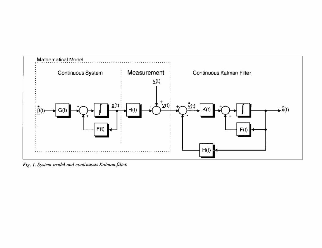
The structure of (34) shows that the Kalman
Filter incorporates a model of the signal and a
correction term, which is an optimally weighted
error = K(t)(dyt − ztdt) (see Fig. 1).
98

It remains to find an explicit expression for K(t).
Here we see an interplay between filtering theory
and linear systems theory. The solution of (34)
can be written as
xt =∫ t
0(t, s)K(s)dνs (35)
where (t, s) is the transition matrix
corresponding to F .
99

From (32) and (35)
(t, s)K(s) =∂
∂sE(xtν
′s)
and hence
K(t) =∂
∂sE(xtν
′s) |s=t .
Some further calculations, using the fact that
xt ⊥ Hws , show that
K(t) = P (t)H ′ ,
where P (t) = E(xtx′t), xt = xt − xt.
100
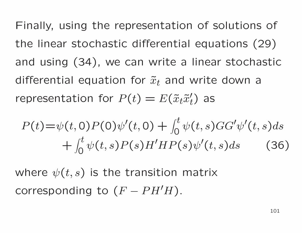
Finally, using the representation of solutions of
the linear stochastic differential equations (29)
and using (34), we can write a linear stochastic
differential equation for xt and write down a
representation for P (t) = E(xtx′t) as
P (t)=ψ(t,0)P (0)ψ′(t,0) +∫ t
0ψ(t, s)GG′ψ′(t, s)ds
+∫ t
0ψ(t, s)P (s)H ′HP (s)ψ′(t, s)ds (36)
where ψ(t, s) is the transition matrix
corresponding to (F − PH ′H).
101

There is again a role of linear systems theory
evident here. Differentiating w.r. to t, we get a
matrix differential equation for P (t), the matrix
Ricatti equation
dP
dt= GG′ − P (t)H ′HP (t) + FP (t) + P (t)F ′
P (0) = cov(x0) = P0 . (37)
Note that K(t) = P (t)H ′ is deterministic and
does not depend on the observation process yt,
and hence can be pre-computed.
102

The approach to the solution of the Wiener
Filtering Problem consists in studying the
equilibrium behavior of P (t) as t→ ∞. There is
again a beautiful interplay between the infinite
time behavior of the filter and the structural
properties of (29). One can prove that if the
pair (F,G) is stabilizable and (H,F ) is detectable
then P (t) → P as t→ ∞ where P is the unique
non-negative solution to the algebraic Ricatti
equation corresponding to (37) and that
F − PH ′H is a stability matrix.103

Thus the filter is stable, in the sense that the
error covariance converges to the optimal error
covariance for the stationary problem even if F is
not a stability matrix. For the linear systems
concepts introduced here and the proof of the
above results the reader may consult Wonham
[10].
104

In a Control context, the controls enter the filter
as a separate input and one needs to study the
controlled filtering problem. This is important
for proving the Separation Principle.
105

On Some Connections between
Nonlinear Filtering, Information Theory,
and Statistical Mechanics
Sanjoy K. Mitter
Laboratory for Information and Decision Systems
Massachusetts Institute of Technology
Joint work with Nigel Newton, University of Essex

Some Connections between Information Theory, Filtering
and Statistical Mechanics
Variational Approach to Bayesian Estimation
Stochastic Control Interpretation of Nonlinear Filtering
106

Preliminaries
X,Y discrete random variables with joint distribution PXY
and marginals PX and PY
I(X; Y ) = EPXY
logPXY
PX ⊗ PY
: Mutual Information
Average measure of dependence of two random variables
Mutual Information is an example of the general notion of
relative entropy between two measures µ and ν on some
probability space ( ,F , P ) (discrete for the moment)
h(µ|ν) = Eµ log
(
µ
ν
)
107

Properties:
(i) h(µ|ν) ≥ 0
(ii) h(µ|ν) = 0⇔ µ = ν
(iii) h(µ|ν) jointly convex in µ, ν
(But, not symmetric). Defines a pseudo-distance be-
tween two measures µ and ν.
We will have to deal with random variables in a more
general setting.
108

Nonlinear Dynamical Systems
forced by (scaled) white noise
dxt
dt= b(xt) + σ(xt)vt ,
where vt: Brownian motion and vt = white noise, formal
derivative of Brownian motion
Rewrite as Integral equation
xt = x0 +∫ t
0b(xs)ds+
∫ t
0σ(xt)vtdt
= x0 +∫ t
0b(xs)ds+
∫ t
0σ(xt)dvt ← Ito integral
109

We want to think of x(·) := X as a map (random vari-
able) from ( ,F , P ) to (X ,B(X ) where X = C(0, T ;R)and B(X ) is the Borel field associated with X . We call
the probability measure of X ∈ P(X ) the path space
measure
T
t
Xt ( ).
X is a random trajectory
Sometimes, we would want to look at these random tra-
jectories “through” a different measure P (instead of P )
in order for it to “appear” differently, for example, tra-
jectories of Brownian Motion.110

Gibbs Measures:
Variational Characterization for Finite Systems
(H.O. Georgii: Gibbs Measures and Phase Transitions, Chapter 15)
Let S = finite set, and E = state space, finite set and
let = ES, finite.
Let be any potential, and H =∑
A⊂SA(w) be the
associated Hamiltonian
The unique Gibbs measure for is given by
ν(ω) = Z−1 exp[−H(ω)] , ω ∈where
Z =∑
ω∈exp[−H(ω)] : Partition function
111

For each probability measure µ on ,
µ(H) =∑
ω∈µ(ω)H(ω) and h(µ) = −
∑
ω∈µ(ω) logµ(ω)
be the Energy and Entropy associated with µ
Then
µ(H)− h(µ) + logZ = h(µ|ν) ≥ 0
h(µ|ν) = 0⇔ µ = ν
F(µ) = µ(H)− h(µ) : Free Energy
F(ν) = − logZ
112

Generalization of these ideas to infinite systems leads to
characterization of translation-invariant Gibbs measures
as minimization of Specific Free Energy. A modification
of these ideas (using Exchangeability) leads to a proof
of the Noisy Channel Coding Theorem (BSC).
Variational Bayes and a Problem of Reliable Communication, Part II,
N. Newton, S.K. Mitter, J. Stat. Mech.: Theory and Experiment,
Iss. 11, pp. 111008, 2012
113

Information Theory, Filtering and Statistical Mechanics
(Xt)t≥0 Markov Process, time homogeneous
P (Xt ∈ B|Xr, r ∈ [0, s]) = π(t− s,Xs, B) 0 ≤ s ≤ t ≤ T
Pt is the distribution of Xt with density pt
Pt(B) = P (Xt ∈ B) =∫
Bpt(x)λx(dx) λx : ref. measure
Diffusion
(Ap)(x) =1
2
∑
i,j
∂2(ai,jp)
∂xi∂xj(x)−
∑
i
∂
∂xi(bip)(x) on R
d
Xt = X0 +∫ t
0b(Xs)dt+
∫ t
0σ(Xs)dvs
a = σσ′
114

Relative Entropy
h(µ|λ) =∫
Xq(x) log q(x)λ(dx) µ has density q w.r.t. λ
= +∞ otherwise
〈f, λ〉 =∫
Xf(x)λ(dx)
x: statistical mechanical system, associated with (Xt)t≥0
Pt: state of x at time t
PSS: unique invariant measure with density pSS
Internal Energy EX(Pt) = 〈Hx, Pt〉
Entropy Sx(Pt) = −h(Pt|λx)
Free Energy FX(Pt) = Ex(Pt)− Sx(Pt)
Energy Function Hx(x) = − log pSS(x)
Choice assures Energy Function is a Gibbs measure for x
115

Proposition:
(i) Unique minimizer of Free Energy of x is PSS
(ii) Fx(PSS) = 0
(iii) Free Energy of x is non-increasing
Proof.
F(x)(Pt) = h(Pt|PSS)⇒ (i) and (ii)
To prove (iii), P(2)s,t = two point joint distribution
P(2)s,t (B,C) = P (Xs ∈ B,Xt ∈ C) =
∫
Bπ(t− s,X,C)Ps(dx)
P(2)s,t,SS = joint distribution when Ps = PSS
Chain rule for Relative Entropy
116

h(P(2)s,t |P
(2)s,t,SS)
= h(Pt|PSS) +∫
h(˜(t, s, x, · )|˜SS(t− s, x, · ))Pt(dx)
≥ h(Pt|PSS)(Chain Rule)
where ˜(t, s, x, · ) = regular (Xt = x)-conditional dis-
tribution for Xs under the joint distribution P(2)s,t and
˜SS(t − s, x, · ) is the equivalent under the joint distri-
bution P(2)s,t,SS.
117

x: one component of a two-component energy conserv-
ing system that includes a unit temperature heat bath
with which x interacts
If Entropy of system = Entropy of the sum of two com-
ponents then any change in this entropy resulting from
the evolution of Pt = neg. of corresponding change in
Fx(Pt)
PSS: unique invariant measure with density pSS
Proposition: Entropy of closed system is maximized by
PSS and non-decreasing
Assertion (iii) in Proposition can be thought of as a Sec-
ond Law of Thermodynamics for x
118

Observations (Interaction with Measurements)
Yt =∫ t
0g(Xs)ds+Wt
E
[
∫ t
0|g(Xt)|2dt <∞
(Zt|t ∈ [0, T ]): regular conditional probability of Xt
given (Ys|0 ≤ s ≤ t)
ξt: density
ξt(x) = ξ0(x) +∫ t
0(Aξs)(x)ds+
∫ t
0ξs(x)(g(x)− 〈g, Zs〉)′dνs
(1)
νt = Yt −∫ t
0〈g, Zs〉)ds Innovations
119

We want to study the Information flow from the initial
state and running observations (Ys|0 ≤ s ≤ t) into the
regular conditional distribtution
PXt|(Ys,0≤s≤t) ( · , y)
(the filter).
Is this flow, conservative, dissipative?
120

Information Theoretic Quantities
S(t) = I((Xs, s ∈ [0, T ]);Ys, s ∈ [0, t]) = supply
C(t) = I((Xs, s ∈ [t, T ]);Ys, s ∈ [0, t]) = storage
D(t) = S(t)− C(t) = dissipation
Proposition
S(t) = C(0) +1
2E∫ t
0|g(Xs)− 〈g, Zs〉|2ds
C(t) = I(Xt;Zt) = Eh(Zt|Pt)
D(t) = EI((Xs, s ∈ [0, t]);Ys, s ∈ [0, t]|Xt)
121

.S(t) =
1
2E|g(Xt)− 〈g, Zt〉|2 (2)
.D(t) = E
Apt
ptlog pt −
Aξt
ξlog ξt
(Xt) (3)
Sensitivity of Mutual Information C(t) to the randomiza-
tion in the dynamics of the signal
For Diffusions.D(t) =
1
2E∇ log
ξt
pt
′a∇ log
ξt
pt
(Xt)
Rate of change of storage can be found by application
of Ito’s rule to
ξt log
ξt
pt
(Xt)
122

Equations (2) and (3) show that the supply of informa-
tion is associated with the second integral in (1)∫ t
0ξs(x)(g(x)− 〈g, Zs〉)′dνs
and the dissipation associated with the first integral in (1)∫ t
0(Aξs)(x)ds
.S(t) = signal to noise power ratio of the observations
and.D(t) = measure of the rate at which X forgets its past
123

Notes on Proof:
C(t) = I(Xt;Ys; s ∈ [0, t]) = I(Xt;Zt)
S(t) = E logMt ,
where
Mt =dZ0
dP0(x0) exp
(
∫ t
0g(xs)− 〈g, Zs〉
)′dws
+1
2
∫ t
0|g(xs)− 〈g, Zs〉|2ds)
Interactive Statistical Mechanics
The conditional distribution Zt takes into account the
partial observations available up to time t. Define an
energy function for X|Z in such a way that Zt is the
minimum free-energy state at time t.124

Let (Zt) be a stochastic process that satisfies the filter
equation (Zt 6= Z0) with density (ξt).
Eξt corresponds to a state of X and satisfies the Fokker–
Planck equation.
Define energy function
HX|Z(x, t) = − log ξt(x)
EX|Z(Zt, t) = 〈HX|Z( · , t), Zt〉
SX|Z(Zt) = SX(Zt) = −h(Zt|λX)
FX|Z(Zt, t) = EX|Z(Zt, t)− SX|Z(Zt)
125
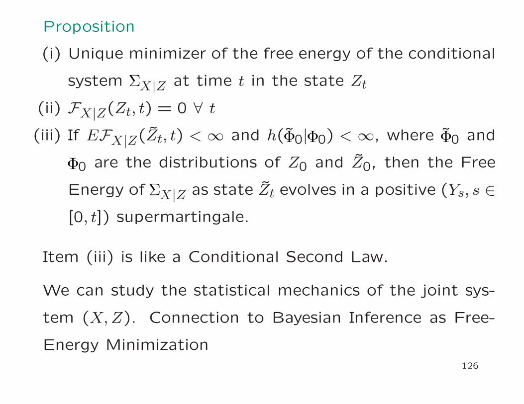
Proposition
(i) Unique minimizer of the free energy of the conditional
system X|Z at time t in the state Zt
(ii) FX|Z(Zt, t) = 0 ∀ t
(iii) If EFX|Z(Zt, t) < ∞ and h(˜0| 0) < ∞, where ˜0 and
0 are the distributions of Z0 and Z0, then the Free
Energy of X|Z as state Zt evolves in a positive (Ys, s ∈[0, t]) supermartingale.
Item (iii) is like a Conditional Second Law.
We can study the statistical mechanics of the joint sys-
tem (X,Z). Connection to Bayesian Inference as Free-
Energy Minimization126

Data Assimilation ≡ Path Estimation or Filtering
or Prediction
Nonlinear Filtering: The Innovations Viewpoint
Stochastic Partial Differential Equation for the Evolution
of the Conditional Density
The Variational Viewpoint:
Information-theoretic Interpretation
Connections to Stochastic Control
Non-equilibrium Statistical Mechanics
127

2. A Variational Formulation of Bayesian Estimation
Let ( ,F , P ) be a probability space, (X,X ) and (Y,Y)Borel spaces, and X : → X and Y : → Y measurable
mappings with distributions PX, PY and PXY on X , Yand X × Y, respectively. Suppose that:
(H1) there exists a σ-finite (reference) measure, λY , on Ysuch that PXY ≪ PX ⊗ λY . (This could be PY itself.)
Let Q : X × Y → [0,∞) be a version of the associated
Radon-Nikodym derivative, and
Y =
y ∈ Y : 0 <∫
XQ(x, y)PX(dx) <∞
; (4)
128

then Y ∈ Y and PY (Y) = 1. Let H : X×Y → (−∞,+∞]
be defined by
H(x, y) = − log(Q(x, y)) if y ∈ Y
(5)0 otherwise :
then PX|Y : X ×Y → [0,1], defined by
PX|Y (A, y) =
∫
Aexp(−H(x, y))PX(dx)
∫
Xexp(−H(x, y))PX(dx)
, (6)
is a regular conditional probability distribution for X given
Y ; i.e.
129
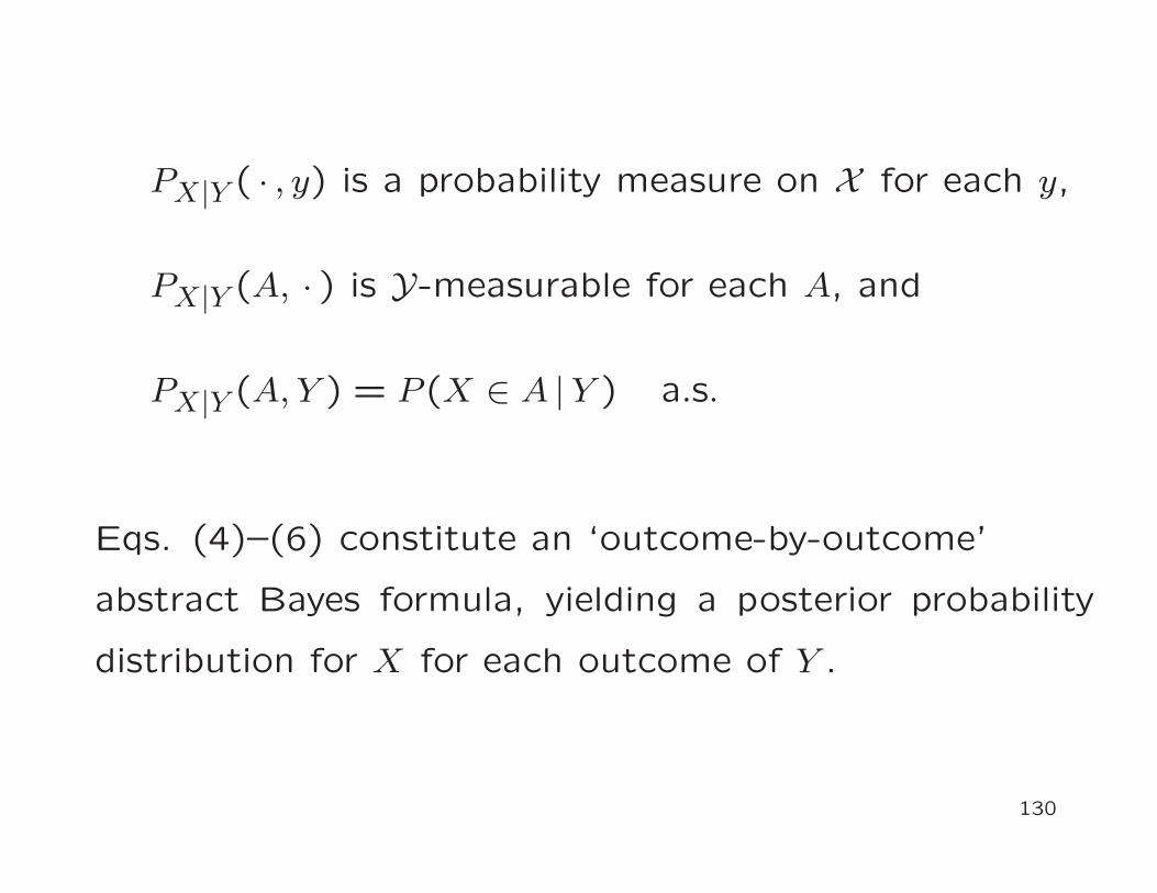
PX|Y ( · , y) is a probability measure on X for each y,
PX|Y (A, · ) is Y-measurable for each A, and
PX|Y (A, Y ) = P (X ∈ A |Y ) a.s.
Eqs. (4)–(6) constitute an ‘outcome-by-outcome’
abstract Bayes formula, yielding a posterior probability
distribution for X for each outcome of Y .
130

Let P(X ) be the set of probability measures on (X,X ),
and H(X) the set of (−∞,+∞]-valued, measurable func-
tions on the same space. For PX, PX ∈ P(X ) and H ∈H(X), we define
h(PX | PX) =∫
X
log
(
dPX
dPX
)
dPX if PX ≪ PX and the integral exists
(7)+∞ otherwise,
i(H) = − log
(∫
X
exp(−H)dPX
)
if 0 <
∫
X
exp(−H)dPX <∞(8)
−∞ otherwise,
〈H, PX〉 =
∫
X
HdPX if the integral exists
(9)+∞ otherwise.
131

It is well known that the relative entropy h(PX | PX) can
be interpreted as the information gain of the probability
measure PX over PX. In fact, any version of − log(dPX/dPX)
is a generalisation of the Shannon information for X. For
almost all x, it is a measure of the ‘relative degree of sur-
prise’ in the outcome X = x for the two distributions PX
and PX. Thus, h(PX | PX) is the average reduction in
the degree of surprise in this outcome arising from the
acceptance of PX as the distribution for X, rather than
PX.
132

If we interpret exp(−H) as a likelihood function for X, as-
sociated with some (unspecified) observation, then H(x)
is the ‘residual degree of surprise’ in that observation
if we already know that X = x, and i(H) is the ‘total
degree of surprise’ in that observation, i.e. the informa-
tion in the unspecified observation if all we know about
X is its prior PX. In what follows we shall call H(X)
the X-conditional information in the unspecified obser-
vation, and i(H) the information in that observation. (Of
course, H(X, y) and, respectively, i(H( · , y)) are the X-
conditional information and, respectively, information in
the observation that Y = y.)
133

Theorem 1
(i) i ((H( · , y)) = minPX[h(PX |PX) + 〈H( · , y), PX〉]
(ii) h(PX|Y ( · , y)|PX) = maxH
i(H)− 〈H, PX|Y ( · , y)
(iii) PX|Y ( · , y) is the unique minimizer in (i)
(iv) If H∗ is a maximizer in (ii), then ∃K ∈ R s.t. H∗(X) =
H(X, y) +K

Conceptualization
Information Processing over and above that in prior PX
In (i): Source of additional information is Y = y
Bayes Formula: Extracts info. pertinent h(PX|Y ( · , y)|PX)
and leaves residual 〈H,PX|Y 〉.
Input information is held in likelihood exp(−H( · , y)) and
extracted information in PX|Y ( · , y)
134
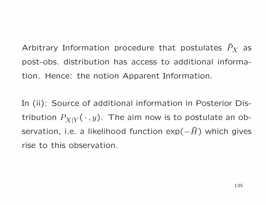
Arbitrary Information procedure that postulates PX as
post-obs. distribution has access to additional informa-
tion. Hence: the notion Apparent Information.
In (ii): Source of additional information in Posterior Dis-
tribution PX|Y ( · , y). The aim now is to postulate an ob-
servation, i.e. a likelihood function exp(−H) which gives
rise to this observation.
135

Input Information
h(
PX|Y ( · , y)|PX
)
is merged with the residual information of the postulated
observation
〈H, PX|Y ( · , y)〉 :
Result ≥ i(H)
With equality ⇔ Obs. is compatible with PX|Y
i(H)− 〈H, PX|Y ( · , y)〉= Inf. in Postulated Obs.
compatible with PX|Y ( · , y)
Compatible Inf. of exp(−H)
136
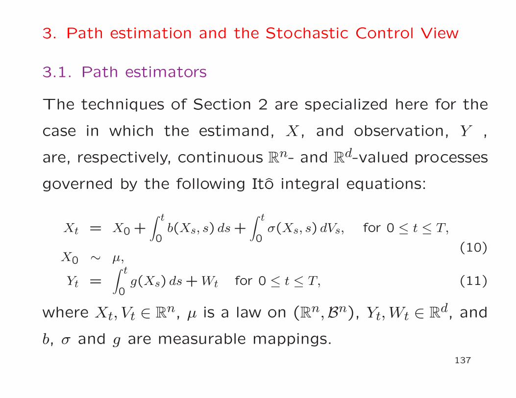
3. Path estimation and the Stochastic Control View
3.1. Path estimators
The techniques of Section 2 are specialized here for the
case in which the estimand, X, and observation, Y ,
are, respectively, continuous Rn- and R
d-valued processes
governed by the following Ito integral equations:
Xt = X0 +
∫ t
0b(Xs, s) ds+
∫ t
0σ(Xs, s) dVs, for 0 ≤ t ≤ T,
(10)X0 ∼ µ,
Yt =
∫ t
0g(Xs) ds+Wt for 0 ≤ t ≤ T, (11)
where Xt, Vt ∈ Rn, µ is a law on (Rn,Bn), Yt,Wt ∈ R
d, and
b, σ and g are measurable mappings.
137

Under suitable regularity conditions, these equations will
be unique in law and have a weak solution
[ ,F , (Ft), P, (V,W ), (X,Y )] ,
i.e., a filtered probability space supporting an (n + d)-
dimensional Brownian motion (V,W ) and an (n + d)-
dimensional semimartingale (X,Y ) such that (10) and
(11) are satisfied for all t. The abstract spaces (X,X )
and (Y,Y) now become the spaces (C([0, T ];Rn),BT) and
(C([0, T ];Rd),BT) of continuous functions, topologized
by the uniform norm. We continue to use the notation
(X,X ) and (Y,Y), though, for the sake of brevity.
138

Let λY be Wiener measure on (Y,Y). Under suitable
conditions on µ, b, σ and g, we might expect the tech-
nical hypothesis for Theorem 1 to be satisfied and the
mutual information, E log[dPXY /d(PX⊗λY )(X,Y )], to be
finite. This will allow us to proceed as in Section 2 to
construct a function H on X × Y , and a corresponding
regular conditional probability, PX|Y , holds for all y. Fur-
thermore, if we can show that PX|Y ( · , y) ∼ PX, then we
shall be able to construct a continuous, strictly positive
martingale My on such that
My,t = E
dPX|Y ( · , y)dPX
(X) | FXt
for 0 ≤ t ≤ T,
139

where (FXt ) is the filtration generated by the process X.
It will then follow from the Cameron–Martin–Girsanov
theory that
My,t = My,0 exp
(
∫ t
0U ′y,s(dXs − b(Xs, s) ds)
−12
∫ t
0|σ(Xs, s)
′Uy,s|2 ds)
(12)
for some progressively measurable, Rn-valued process Uy.
PX|Y ( · , y) will then be the distribution of a controlled
process, Xy, satisfying an equation like (10), but with a
different initial law, and with a control term, σσ′(Xs, s)Uy,s,
entering the drift coefficient.
140

Xt = X0+∫ t
0b(Xs, s)ds+
∫ t
0σσ′(Xs, s)Uy,sds+
∫ t
0σ(Xs, s)dvs
with 0 ≤ t ≤ T .
The use of the progressively measurable control U instead
of Uy will result in a process X having a distribution whose
apparent information relative to [PX, H( · , y)] is greater
than or equal to that of Xy. Thus, at least in part, the
variational characterization of Section 2 will become a
problem in stochastic optimal control.
141

It turns out that the Path Estimation Problem can be
solved in the following way:
Run a backward likelihood filter starting at the end time
to estimate the initial distribution of the state. In the
process, some information is dissipated at an optimal
rate governed by the Fisher Information†.
The dissipated information is recovered by running a for-
ward optimal stochastic control problem. The resulting
optimal path-space measure is the conditional path esti-
mator.
†Mitter, S.K. and Newton, N.J., “Information and Entropy Flow in the Kalman-Bucy Filter,”
J. of Stat. Phys 118 (2005), pp. 145-176.
142

3.2. Stochastic Control Problem
Consider the following controlled equation
Xt = θ +∫ t
0
(
b(Xs, s) + a(Xs, s)u(Xs, s))
ds+∫ t
0σ(Xs, s) dVs, (13)
where the initial condition, θ, is non-random. Let U be
the set of measurable functions u : Rn× [0, T ] → Rn with
the following properties:
(U1) u is continuous;
(U2) E u = 1, where
u = exp
(
∫ T
0u′σ(Xθ,0
t , t) dVt −1
2
∫ T
0|σ′u(Xθ,0
t , t)|2 dt)
, (14)
and ( ,F , P ), V and Xz,s are the corresponding
martingales (Girsanov).
143

Lemma. If b and σ satisfy the technical hypothesis and
u ∈ U then (13) has a weak solution and is unique in law.
Let (˜, F , (Ft), P , X, V ) be a weak solution of (13) for
some u ∈ U. We define the cost for controls in U as the
apparent information of the resulting distribution of X,
PX. This is measured relative to the prior Pθ,0X (the dis-
tribution of Xθ,0), and Hp(0, T, θ, · , y) [the Hamiltonian:
see Section 3].
144

J(u, θ, y) = h(PX |P θ,0X ) + 〈Hp(0, T, θ, · , y), PX〉
=1
2E
∫ T
0|σ′u(Xt, t)|2 dt− y′Tg(θ) +
1
2E
∫ T
0|g(Xt)|2 dt
(15)
− E
∫ T
0(yT − yt)
′(Lg +Dg)(Xt, t) dt
if the integrals exist
+∞ otherwise,
where L is the differential operator associated with X,
L =∑
i
bi∂
∂zi+
1
2
∑
i,j
ai,j∂2
∂zi∂zj,
and D is the row-vector jacobian operator, D = [∂/∂z1 ∂/∂z2 · · · ∂/∂zn].The cost functional has a more appealing form in the special case
that the observation path, y, is everywhere differentiable:
J(u, θ, y) =1
2E
∫ T
0
(
|σ′u(Xt, t)|2 + |yt − g(Xt)|2)
dt− 1
2
∫ T
0|yt|2 dt.
(16)
145

This involves an ‘energy’ term for the control and a
‘least-squares’ term for the observation path fit. These
correspond to the two terms in Bayes’ formula represent-
ing the degrees of match with the prior distribution and
the observation path. The optimal control problem (13),
(16) can be thought of as a type of energy-constrained
tracking problem. The optimal control, under which the
distribution of X is the regular conditional probability dis-
tribution PX|Y ( · , y), is derived in the following theorem.
146
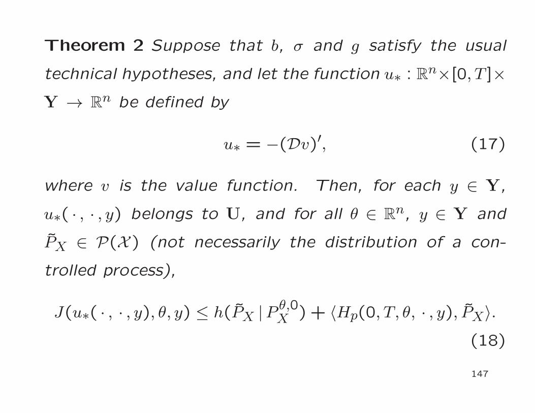
Theorem 2 Suppose that b, σ and g satisfy the usual
technical hypotheses, and let the function u∗ : Rn×[0, T ]×Y → R
n be defined by
u∗ = −(Dv)′, (17)
where v is the value function. Then, for each y ∈ Y,
u∗( · , · , y) belongs to U, and for all θ ∈ Rn, y ∈ Y and
PX ∈ P(X ) (not necessarily the distribution of a con-
trolled process),
J(u∗( · , · , y), θ, y) ≤ h(PX |P θ,0X ) + 〈Hp(0, T, θ, · , y), PX〉.
(18)
147

We now consider the special case in which y is differ-
entiable with Holder continuous derivative, b and g are
bounded, and there exists an ǫ > 0 such that
z′a(z)z ≥ ǫ|z|2 for all z, z ∈ Rn. (19)
In this case ρ is continuously differentiable with respect
to s, twice continuously differentiable with respect to z,
and by a standard extension of the Feynman–Kac formula
satisfies the following p.d.e.
∂ρ
∂s+Lρ+
(
y − 1
2g
)′gρ = 0 on R
n×(0, T ), ρ( · , T, y) = 1.
(20)
148

Since v = − log(ρ), the value function, v, satisfies
∂v
∂s+ Lv − 1
2Dva(Dv)′ −
(
y − 1
2g
)′g = 0
on Rn × (0, T ), v( · , T, y) = 0. (21)
149

3.3. The Inverse Problem
The variational characterization of the inverse problem
[parts (ii) and (iv) of Theorem 1, Section 3] can also be
applied to the path estimator. This involves choosing a
likelihood function to be compatible with the (given) reg-
ular conditional probability distribution, PX|Y ( · , y). Ear-
lier, we minimized apparent information over probability
measures corresponding to weak solutions of the con-
trolled equation. Here, we maximize compatible infor-
mation over (negative) log-likelihood functions, H, that
give rise to posterior distributions of this type.
150

Let ( ,F , P ), µ, V , and X be as defined previously. For
each probability measure on Rn, µ, with µ≪ µ, and each
continuous u satisfying (U2) for all θ, let H be a mea-
surable function such that
H(X) = − log
dPX
dPX
(X)
+K
(22)
= − log
dµ
dµ(X0)
−∫ T
0u′σ(Xt, t) dVt
+1
2
∫ T
0|σ′u(Xt, t)|2 dt+K,
where K ∈ R and PX is as defined previously.
We shall assume that µY ( · , y) ≪ µ. The term K in
(22) is the information in the associated (unspecified)
observation.151

Integral log-likelihood functions of the form (22) can be
thought of as being associated with observations that
are ‘distributed in time’, in that information from them
gradually becomes available as t increases.
The characterization of PX|Y in terms if stochastic con-
trol can be used to express the compatible information
corresponding to H, as follows:
G(H, y) = K − 〈H , PX|Y ( · , y)〉= K + h(µY ( · , y) |µ)− h(µY ( · , y) | µ) (23)
+∫ T
0
∫
Rn
(
u∗ −1
2u
)′au(z, t, y)
· PX|Y (χ−1t (dz), y) dt.
152

Log-likelihood functions of the form (22) could come
from many different types of observation.
The only constraints placed on u here are that it be
continuous and satisfy (U2) for all θ. We could further
constrain it to take the form
u(z, s) = −(Dv)′(z, s, y),where
v(z, s, y) = − logE exp
∫ T
s
(
˙yt −1
2g(X
z,st )
)′g(X
z,st ) dt
,
for appropriate g and y. This would correspond to ob-
servations of the ‘signal-plus-white-noise’ variety similar
to (11), but with ‘controlled’ observation function and
path, g and y.
153

This would show the effects of errors in the observa-
tion function or approximations of the observation path.
Under appropriate regularity conditions v will satisfy the
following partial differential equation:
−∂v∂t
= Lv−1
2Dva(Dv)′−
(
˙yt −1
2g
)′g; v( · , T ) = 0. (24)
Thus one interpretation of the inverse problem involves
the infinite-dimensional, deterministic optimal control in
reversed time, with control (g, y), and payoff
(g, y) =∫ T
0
∫
RnDva
(
u∗ −1
2(Dv)′
)
(z, t, y)
· PX|Y (χ−1t (dz), y) dt. (25)
154

The optimal trajectory for this dual problem, v( · , · , y) is
a time-reversed likelihood filter for X given Y , and the
measure, exp(−v(z, s, y))PX(χ−1s (dz)) is an un-normalized
regular conditional probability distribution for Xs given
observations (Yt − Ys, s ≤ t ≤ T ), which coincides with
that provided by the Zakai equation for the time-reversed
problem. This provides an information-theoretic expla-
nation of the connection between nonlinear filtering and
stochastic optimal control used in †, as well as widening
its scope. A detailed account of this, and the information
processing aspects of nonlinear filters and interpolators
can be found in ∗. For a somewhat different problem
involving optimization over observation functions, see #.155

†W.H. Fleming and S.K. Mitter,
“Optimal control and nonlinear filtering for nondegenerate diffusion processes,”
Stochastics 8 (1982), pp. 63–77.
∗Mitter, S.K. and Newton, N.J., “Information and Entropy Flow in the Kalman-Bucy Filter,”
J. of Stat. Phys 118 (2005), pp. 145-176.
#B.M. Miller and W.J. Runggaldier, “Optimization of observations: a stochastic control approach,”
SIAM J. Control Optim. 35 (1997), pp. 1030–1052.
156

Extensions to State Process described by
Partial Differential Equation (Lattice)
See recent work of R. Von Handel and collaborators
Infinite-Lattice, Infinite-time Behavior of Filter
157

CONCLUSION
• Integration of Stochastic Control and
Information Theory
• Nonequilibrium Statistical Mechanics
• Application Areas
Sensor Networks and Monitoring
Energy Harvesting
158