Embed Size (px)
Citation preview
On Solution Concepts ofAssignment Games
Inauguraldissertation zur Erlangung des Grades
eines Doktors der Wirtschaftswissenschaften (Dr. rer. pol.)an der Fakultat fur Wirtschaftswissenschaften
der Universitat Bielefeld
vorgelegt von
Dipl.-Wirt. Math. Maike Hoffmann
Januar 2008

1. Gutachter: Prof. em. Dr. Joachim Rosenmuller
Institut fur Mathematische Wirtschaftsforschung (IMW)
Universitat Bielefeld
2. Gutachter: Prof. Dr. Walter Trockel
Institut fur Mathematische Wirtschaftsforschung (IMW)
Universitat Bielefeld
Acknowledgment
First of all I wish to thank my doctoral supervisors Prof. Dr. Joachim Rosenmuller
and Prof. Dr. Walter Trockel for many interesting discussions during the last years.
For the joint work on the paper”The shapley value of exact assignment games“
I want to thank Prof. Dr. Peter Sudholter. It was him who convinced me to publish
the results in the”International Journal of Game Theory“.
Financial support from the Deutsche Forschungsgemeinschaft (DFG) through a
scholarship within the International Research Training Group ’Economic Behav-
ior and Interaction Models’ at Bielefeld University is gratefully acknowledged.
Last but not least, many thanks to all friends who encouraged me to continue this
thesis at times when I was in doubt to be on the right way. Without this benefit
and numerous conversations, this thesis would not have been finished. In particular
I would like to thank Monika Bier, Krasen Dimitrov, Claus-Jochen Haake, Evan
Shellshear, Sebastian Kohne and Julia Zakotnik for their support.
Contents
1 Introduction 4
2 Cooperative Games and Solution Concepts 9
2.1 Introduction . . . . . . . . . . . . . . . . . . . . . . . . . . . . . . . . 9
2.2 Cooperative Games with Transferable Utility . . . . . . . . . . . . . . 10
2.2.1 Classes of Cooperative Games . . . . . . . . . . . . . . . . . . 12
2.3 Solution Concepts . . . . . . . . . . . . . . . . . . . . . . . . . . . . . 14
2.3.1 Some Properties of Solution Concepts . . . . . . . . . . . . . . 16
2.3.2 Core and Least Core . . . . . . . . . . . . . . . . . . . . . . . 17
2.3.3 Nucleolus and Modified Nucleolus . . . . . . . . . . . . . . . . 22
2.3.4 The Shapley Value . . . . . . . . . . . . . . . . . . . . . . . . 26
2.4 Assignment Games . . . . . . . . . . . . . . . . . . . . . . . . . . . . 29
2.4.1 The Definition . . . . . . . . . . . . . . . . . . . . . . . . . . . 29
2.4.2 Special Classes of Assignment Games . . . . . . . . . . . . . . 33
2.4.3 Modified Nucleolus of Assignment Games . . . . . . . . . . . . 36
2.5 Strong Nullplayer Property . . . . . . . . . . . . . . . . . . . . . . . . 37
3 The Shapley Value and the Core 42
3.1 Introduction . . . . . . . . . . . . . . . . . . . . . . . . . . . . . . . . 42
3.2 Partially Average Convex Games . . . . . . . . . . . . . . . . . . . . 43
3.2.1 Partially Average Convex Assignment Games . . . . . . . . . 44
3.3 The Shapley Value as an Element of the Core . . . . . . . . . . . . . 45
3.4 Exact Assignment Games . . . . . . . . . . . . . . . . . . . . . . . . 46
3.4.1 The Shapley Value of Exact Assignment Games . . . . . . . . 49
2
CONTENTS 3
3.4.2 Games with a Large Core . . . . . . . . . . . . . . . . . . . . 55
3.4.3 Some Examples . . . . . . . . . . . . . . . . . . . . . . . . . . 58
3.5 Non-exact Assignment Games . . . . . . . . . . . . . . . . . . . . . . 59
4 The Least Core of the Dual Assignment Game 66
4.1 Introduction . . . . . . . . . . . . . . . . . . . . . . . . . . . . . . . . 66
4.2 The Least Core of C-convex Games . . . . . . . . . . . . . . . . . . . 67
4.2.1 Extreme Points of the Least Core . . . . . . . . . . . . . . . . 70
4.3 Properties of the Least Core of the Dual Assignment Game . . . . . . 72
4.4 Convex Assignment Games . . . . . . . . . . . . . . . . . . . . . . . . 76
4.4.1 Properties of the Least Core . . . . . . . . . . . . . . . . . . . 77
4.4.2 Assignment Games with a Stable Core . . . . . . . . . . . . . 81
4.5 Symmetric and Exact Assignment Games . . . . . . . . . . . . . . . . 83
4.5.1 On some Solution Concepts . . . . . . . . . . . . . . . . . . . 83
4.5.2 Characteristics of the Least Core . . . . . . . . . . . . . . . . 89
5 Assignment Games induced by 2 × 2 matrices 92
5.1 Introduction . . . . . . . . . . . . . . . . . . . . . . . . . . . . . . . . 92
5.2 The Least Core of Dual Assignment Games . . . . . . . . . . . . . . . 92
5.2.1 Extreme Points of the Least Core . . . . . . . . . . . . . . . . 95
5.3 The Core . . . . . . . . . . . . . . . . . . . . . . . . . . . . . . . . . 97
5.3.1 Extreme Points of the Core . . . . . . . . . . . . . . . . . . . 99
5.4 The Intersection of Core and Least Core . . . . . . . . . . . . . . . . 102
5.4.1 Extreme Points of the Intersection . . . . . . . . . . . . . . . 102
6 Conclusions 120
7 Index of Notations 122
References 123
Chapter 1
Introduction
The origins of game theory date back to the year 1944 when the authors von Neu-
mann and Morgenstern published their fundamental book [9] about games and eco-
nomic behavior. Traditionally, this theory deals with situations of conflicts or co-
operation which are described by certain mathematical models. In this context
typically three different forms of models are considered: the models in extensive
form, in normal form and in characteristic function (or coalitional) form. The first
two categories of games are the central topics of non-cooperative game theory. Here,
games with no binding agreements between the players are treated. In contrast to
this kind of models, games in coalitional form permit cooperation and contracts.
Hence, the main focus of cooperative game theory is the examination of groups of
players (coalitions) who coordinate their actions and pool their winnings. On closer
examination, we can observe that these games can be separated into games with
or without transferable utility or more commonly with or without side-payments.
In coalitional games without side-payments players cannot distribute their collec-
tive payoffs. Instead, each coalition is allocated a feasible set of outcomes and a
status quo point, which is the payoff, if the players do not find an agreement on
some feasible outcome. Different solution concepts make suggestions for potential
outcomes. In contrast to coalitional games without side-payments, each coalition of
a cooperative game with side-payments gets a payoff that can be distributed among
its members. The pertinent question how to divide the payoffs among the members
of a formed coalition can be answered with the aid of different solution concepts.
Each concept proposes a set of distributions of the total payoffs to the players.
4
CHAPTER 1. INTRODUCTION 5
One of the most famous solution concepts in cooperative games with side-payments
is the core which was introduced by Gillies [4] in 1953 as an adjunct to the studies
of stable sets. This concept describes the set of Pareto optimal payoff vectors such
that no coalition can raise a warrantable plea. The central issue is the fact that
this concept suggests an empty set or a set that does not have to be a singleton.
A second important solution concept beside the core, is the Shapley value which
was introduced by Shapley [18] in 1953. This concept characterizes the expected
marginal payoffs of the players. In contrast to the core, the Shapley value always
exists and is a singleton. Besides the two solution concepts above, we are also in-
terested in two further concepts which are strongly related. On the one hand we
consider the nucleolus which was introduced by Schmeidler [16] in 1969. This con-
cept minimizes highest dissatisfactions of coalitions. In our context, we will call a
dissatisfaction of a coalition an excess. In addition, we also look at the modified
nucleolus or modiclus which was introduced by Sudholter in a series of papers [27,
29, 30]. In contrast to the nucleolus, the modified nucleolus minimizes the highest
difference of excesses, meaning that the power and the blocking power of a coalition
are taken into account in the same way. By definition, existence and uniqueness of
both solution concepts can be shown.
In this thesis we concentrate on statements of different solution concepts for special
classes of cooperative games with transferable utility. In particular, we are interested
in the class of assignment games which was introduced by Shapley and Shubik [23]
in 1972. Typically, an assignment game describes a one-to-one matching problem
or a model for a two-sided market. Special features of these games are that they
can be described by non-negative matrices and that the player set is separated into
two different types. These properties imply a special structure of assignment games,
which allows many novel results in the context of different solution concepts. For
example, Shapley and Shubik [23] introduced the core of an assignment game as a
non-empty polyhedron of optimal solutions of a corresponding linear program. It
CHAPTER 1. INTRODUCTION 6
can be shown that this linear program only depends on the assignment matrix. A
second fundamental and important result for us is about the nucleolus. In their
paper, Solymosi and Raghavan [25] found an algorithm which calculates the nu-
cleolus of an assignment game. Here, the maximum number of steps depends on
the minimum number of players of both types. In a second paper [26], the authors
characterize the assignment matrix in the case of convex assignment games, exact
assignment games and in the case of assignment games with a stable core. With the
help of these characterizations Raghavan and Sudholter [12] were able to prove that
if the core is stable, then the modified nucleolus is an element of the core.
A relevant task that we tackle in this thesis is to establish a connection between
different solution concepts for assignment games. More precisely, our main interest
is about general results for special classes of games. First of all, we consider the
Shapley value of exact assignment games, before we try to extend our studies to
a more general case. In the next step, we analyze some properties of the modified
nucleolus. In order to do so, we formulate different properties of the least core of
the dual assignment game. Finally, we examine our general results in the case of
assignment games which are induced by a 2 × 2 assignment matrix.
The dissertation is organized as follows. Chapter 2 provides the basic definitions
and solution concepts in the context of cooperative game theory. Before we con-
sider special classes of games, we start with the formal definition of a cooperative
game with transferable utility. Next, we introduce different solution concepts, which
suggest possible distributions of the total payoffs. For different classes of games we
verify specific properties of the solution concepts under consideration. In particu-
lar, we find many important results for assignment games. The special structure
of these games reveals some interesting connections between the different solution
concepts. Finally, we discuss the strong null player property of different solution
concepts. This property allows us to deal with nullplayers so that we can restrict
our attention to assignment games with the same number of players of each type.
CHAPTER 1. INTRODUCTION 7
In Chapter 3 we concentrate on the Shapley value, on the core, and on the rela-
tionship between both concepts. After introducing partially average convex games
we present our most relevant result of this chapter; the Shapley value of an exact
assignment game is an element of the core. For the direct proof we establish an
alternative description of exact assignment games, which proposes a partition of the
worth of the different coalitions. It is illustrated by some examples that exactness
of an assignment game is a necessary condition for our result. Finally, we focus on
non-exact assignment games for which the Shapley value is in the core.
In Chapter 4 we discuss some properties of the least core of the dual assignment
game. After considering some general properties of the least core, we specify these
results in the case of convex assignment games. In this case a delineation of the
least core of the dual assignment game, the Shapley value, and the modiclus is pos-
sible. In the next step we generalize some results for convex assignment games to
assignment games with a stable core. Another absorbing class is the set of exact
assignment games which are induced by a symmetric matrix. Similar to the case of
convex assignment games the calculation of the Shapley value and the modiclus is
possible in a very simple way.
Chapter 5 deals with assignment games with a stable core which are induced by a
2 × 2 matrix. Throughout this chapter we pay attention to the intersection of the
core and the least core of the dual assignment game. Therefore, we emphasize in
the first section the results of the least core of the dual assignment game. We find
a way to compute the extreme points of the least core of the dual assignment game
only with the aid of the assignment matrix. As it turns out, there exists a geometric
presentation of the least core of the dual assignment game. Since the least core is
a subset of a hyperplane, we will see that it is simple to draw this polyhedron. In
the following section, we discuss some properties of the core of assignment games.
In this case, it is also possible to compute the extreme points of the core only with
CHAPTER 1. INTRODUCTION 8
the aid of the assignment matrix. As in the case of the least core, the core is also a
subset of a hyperplane, so that it is very simple to consider the intersection of the
two polyhedrons. More precisely, we find a connection between the extreme points
of the intersection of core and least core and the assignment matrix.
Finally in Chapter 6, we give a short summary of the most important results of the
preceding chapters.
Chapter 2
Cooperative Games and SolutionConcepts
2.1 Introduction
This chapter introduces the basic definitions of cooperative game theory, in partic-
ular the definition of assignment games and some well-known solution concepts like
the Shapley value and the core. Furthermore, important connections between the
solution concepts and the different classes of games are pointed out. In the first
section, we start with the formal definition of a finite n-person cooperative game
with transferable utility. In the next step we look at different classes of cooperative
games, which satisfy some further conditions. Important classes among the additive
games are, the superadditive and the convex games. The second section deals mainly
with different solution concepts for cooperative games. These concepts describe dif-
ferent distributions of the total payoff to the players of the player set. The main
focus of this section is the core, the Shapley value, the nucleolus and the modified
nucleolus. These different concepts supply the different results for different classes
of games. In the next section we consider assignment games, which are models for
two-sided markets. These games were introduced by Shapley and Shubik [23] and
they describe the interaction of two different types of players. With the aid of a
non-negative matrix the worth of the potential interaction of different players can
be computed. We finish this chapter by discussing the strong nullplayer property of
different solution concepts. This property allows us to reduce our attention in the
following chapters to assignment games which are induced by a p × p matrix.
9
CHAPTER 2. COOPERATIVE GAMES AND SOLUTION CONCEPTS 10
2.2 Cooperative Games with Transferable Utility
We start this section with some basic definitions in the context of cooperative games
with finitely many players. For this reason, we define for a finite set I, the power
set P(I) and the complement of a finite subset S ⊆ I. In the following definition
we will consider the power set.
Definition 2.2.1 Let I be a finite set with |I| = n. Then, the set
P(I) = P = {S ⊆ I}
is the power set of I.
The power set of I denotes the set of all subsets of I. One should remark that the
power set P(I) has 2n elements. Another important set is the complement Sc of a
subset S ⊆ I. More formally, we have the following definition.
Definition 2.2.2 Let S ⊆ I, |S| = s, be a subset of a finite set I with |I| = n.
Then, the complement Sc of S is defined by
Sc = {i ∈ I | i /∈ S}.
The complement Sc consists all element of I which are not in the set S. As it can
be shown in a very simple way, the complement Sc has n − s elements.
With the aid of these useful definitions, we are able to define and to explain cooper-
ative games with transferable utility. A cooperative game assigns a value for every
non-empty coalition, that means, we consider a function v from the set of coalitions
to the set of payoffs. This function describes how much collective payoff a set S of
players can gain by forming a coalition. Additionally, it is assumed that the empty
coalition can gain nothing. Summarizing we have the following definition.
Definition 2.2.3 A cooperative game with transferable utility is a triple
(I,P, v) such that I is a finite set and v : P(I) → R is a real-valued mapping with
v(∅) = 0.
CHAPTER 2. COOPERATIVE GAMES AND SOLUTION CONCEPTS 11
The elements of the set I are called players and its power set P(I) denotes the
set of coalitions. Note, that normally the players are named by numbers 1, . . . , n
or by some abstract index set I. The mapping v is called characteristic function.
If the players S ⊆ I agree to cooperate, the profit v(S) from this cooperation is
independent of what the players of coalition Sc can do. The idea of cooperative
games with transferable utility is that the players i ∈ S can split up the payoff v(S)
among the members of the coalition S.
Remark 2.2.4 Sometimes we only use the term cooperative game with transferable
utility for the characteristic function v and not for the triple (I,P, v).
Furthermore, we have in this thesis a short notation for the set of cooperative games.
More formally we have:
Notation 2.2.5 The set of cooperative games with player set I is given by
V ={
v | v : P(I) → R, v(∅) = 0}
.
Since we need to know the payoffs of 2n−1 coalitions to identify a cooperative game,
it is possible to describe a game v ∈ V by a vector z ∈ R2n−1.
Sometimes, there exists some players in the game (I,P, v), who are not really im-
portant for the payoffs of the coalitions. In other words, we can say that the value
v(S) is independent of the membership of this player.
Definition 2.2.6 Let (I,P, v) be a cooperative game. A player i ∈ I is a nullplayer,
if we have
v(S ∪ {i}) = v(S) ∀S ⊆ I.
The profit of every nullplayer i ∈ I is zero, that means, it is the same for the coalition
S if player i joins to the coalition or not.
Before we consider special classes of cooperative games, we define for every game v
a game v? which reflects the preventive power. This game is called dual game and
it assigns to coalition S the complementary worth of the complementary coalition.
CHAPTER 2. COOPERATIVE GAMES AND SOLUTION CONCEPTS 12
Definition 2.2.7 Let (I,P, v) be a cooperative game. The dual game v? of game
v is defined by
v?(S) = v(I) − v(Sc) ∀S ∈ P.
By definition, the dual game v? assigns a little value to a coalition S ⊆ I, if the
complementary coalition Sc ⊆ I is powerful, and vice versa.
2.2.1 Classes of Cooperative Games
Until now we did not specify cooperative games, this means that v does not need
to satisfy further conditions. But sometimes we are interested in characteristic
functions v ∈ V, which have certain properties and special structures. First of all,
we look at the additive games, which are defined as follows.
Definition 2.2.8 A cooperative game v is additive if
v(S) + v(T ) = v(S ∪ T ) ∀S, T ⊆ I, S ∩ T = ∅.
In the case of additive games we only need to know the individual payoff v({i}) of
each single player i ∈ I. Then, the worth of any coalition S ∈ P with more than one
player can be calculated in a simple way by the summing up the individual payoffs
of the single players i ∈ S. More formally, we have in this case for every coalition S
the following equality:
v(S) =∑
i∈S
v({i}).
Thus, it is possible to identify additive games with elements x ∈ Rn and one can
interpret them as distributions of utility. Sometimes additive games are even called
(payoff) allocations or vectors of payoff.
In the following we distinguish between the class of all additive games and the class
of additive games which are non-negative. Therefore, we have the following notation.
Notation 2.2.9 The set of additive games is denoted by A, this means that
A ={
v ∈ V | v is additive}
.
CHAPTER 2. COOPERATIVE GAMES AND SOLUTION CONCEPTS 13
The set of additive games which are non-negative are denoted by A+, this means
that
A+ ={
x ∈ A | x ≥ 0}
.
A second class of games is the class of monotonic games. In this case we have the
following definition.
Definition 2.2.10 Let (I,P, v) be a game. The game v is monotonic if
v(S) ≤ v(T ) ∀S ⊆ T ⊆ I.
Thus, bigger coalitions get at least the same payoff as smaller subcoalitions.
In the next step we want to extend the additive games to a class of games which
yields an incentive of forming coalitions.
Definition 2.2.11 A cooperative game v is superadditive, if
v(S) + v(T ) ≤ v(S ∪ T ) ∀S, T ⊆ I, S ∩ T = ∅
holds true.
In the case of superadditive games collaboration can only help but never hurt. That
means in terms of savings, it is advantageous for disjoint coalitions S and T to form
the union S ∪ T . One of the most important subclasses of superadditive games are
the convex games which are due to Shapley [20] in 1971.
Definition 2.2.12 (Shapley [20])
A cooperative game v is convex if
v(S) + v(T ) ≤ v(S ∩ T ) + v(S ∪ T ) ∀S, T ⊆ I
holds true.
In order to interpret the term of convexness, we examine a second characterization
of convex games. Therefore, we cite the next theorem which can be found in most
of the books about cooperative game theory.
CHAPTER 2. COOPERATIVE GAMES AND SOLUTION CONCEPTS 14
Theorem 2.2.13 Let v be a cooperative game. Then, the following statements are
equivalent:
1. v is convex
2. For i ∈ I we have the following inequality:
v(S ∪ {i}) − v(S) ≤ v(T ∪ {i}) − v(T ) ∀S ⊆ T ⊆ I \ {i}.
The second statement means that the marginal contribution of player i ∈ I to a
coalition S is monotone nondecreasing with respect to set-theoretic inclusion. This
interpretation explains the term convex. During this thesis, it is useful to have a
short notation for convex games.
Notation 2.2.14 We denote the set of convex games with C. More formally, we
have:
C = {v ∈ V | v is convex }.
2.3 Solution Concepts
In this section we study some well-known solution concepts for cooperative games
with transferable utility. The most important concepts are among the core, the
Shapley value, the nucleolus, and the modified nucleolus. Each concept assigns a set
of allocations to a game. So, we can summarize that solution concepts recommend
how v(I) should be divided among the players. In particular, throughout this section
we are interested in solution concepts of convex games. But before introducing the
first solution concept, we start with some special payoff vectors x ∈ A.
Definition 2.3.1 Let v be a game and let x ∈ A be a payoff vector.
1. x is Pareto optimal if x(I) = v(I),
2. x is individually rational (w.r.t. v), if for all i ∈ I we have:
xi ≥ v({i}),
CHAPTER 2. COOPERATIVE GAMES AND SOLUTION CONCEPTS 15
3. x is coalitional rational (w.r.t. v), if for all S ∈ P we have:
x(S) ≥ v(S).
A Pareto optimal payoff vector x is a payoff vector, such that the total payoff v(I)
is distributed to the players i ∈ I. In the case of an individual rational payoff vector
x, every single player i ∈ I prefers the payoff xi instead of the payoff v({i}). If
every coalition prefers the payoff vector x, the payoff vector is called coalitionally
rational.
Now, we want to define some solution concepts. This means that we are looking at
mappings which assign to each game a single vector or a set of feasible payoff vectors.
We can conclude, that in our context, a solution concept is a correspondence
σ : V ⇒ A.
First, we will start with the non-empty set of Pareto optimal allocations, the so-
called set of preimputations. More formally, we have:
Definition 2.3.2 For any cooperative game v the set of preimputations is de-
fined by
X(v) ={
x ∈ A |x(I) = v(I)}
.
In every preimputation the sum of all individual payoffs xi should be equal to the
payoff of the grand coalition v(I). In other words we can say that everything is
divided among the players.
Most solution concepts are special subsets of the set of preimputations. For example
if no player can be forced to accept less than v({i}), we have an imputation.
Definition 2.3.3 The imputation set of a game v is defined by
I(v) ={
x ∈ X(v) | xi ≥ v({i}) ∀i ∈ I}
.
The imputation set is the set of Pareto optimal and individually rational payoff
allocations. It is possible to check in a simple way, if this set is empty or non-empty.
Therefore, one can consider our next remark.
CHAPTER 2. COOPERATIVE GAMES AND SOLUTION CONCEPTS 16
Remark 2.3.4 The imputation set I(v) is non-empty if and only if
v(I) ≥n∑
i=1
v({i}).
2.3.1 Some Properties of Solution Concepts
In this section we want to consider some properties of solution concepts. After that,
we continue our research about some further solution concepts like the core and the
least core. First, we consider solution concepts in which existence and uniqueness
are no problem. This property is called single valued. More formally, we have the
following definition:
Definition 2.3.5 A solution concept σ on a set Γ ⊆ V is single valued if
|σ(v)| = 1 ∀v ∈ Γ.
In the case of a single valued solution concept, we can think of a function σ : V → A
instead of a correspondence. Special single valued solution concepts are the additive
concepts.
Definition 2.3.6 A single valued solution concept σ on Γ ⊆ V is additive if
σ(v1 + v2) = σ(v1) + σ(v2) whenever v1, v2, v1 + v2 ∈ Γ.
Here, it is irrelevant, if one considers the solution concept of the sum of two games
or the sum of the solutions of two games.
Furthermore, it is useful to consider solution concepts which allocate the whole
payoff of the grand coalition to the players.
Definition 2.3.7 A solution concept σ on a set Γ ⊆ V is Pareto optimal if
σ(v) ⊆ X(v) ∀v ∈ Γ.
Now, we want to think about the names of the players. In order to do so, we consider
two games (I,P, v) and (I,P, πv) such that there exists a bijective mapping
π : I → I.
CHAPTER 2. COOPERATIVE GAMES AND SOLUTION CONCEPTS 17
Furthermore, we define with the aid of π a mapping π : V → V by
(π(v))(S) = v(π−1(S)) ∀S ⊆ I.
In particular, we get in the case of additive games x ∈ A the following equality:
(πx)i = xπ−1(i) ∀i ∈ I.
With the help of these definitions, we are able to define our next property of solution
concepts.
Definition 2.3.8 Let Γ ⊆ V be a set of games and let σ be a solution concept on
Γ. The solution concept σ is anonymous if for each game (I,P, v) ∈ Γ and each
bijective mapping π : I → I the equality
σ(πv) = π(σ(v))
holds.
Finally, it can be said, that an anonymous solution concept is permutation invariant.
This property means, that the solution concept is independent of the name of the
players such that a renumbering of the players does not change the payoffs of the
players.
2.3.2 Core and Least Core
In this section we concentrate on two related solution concepts: the core and the
least core. The core was first introduced by Gillies [4,5] as an adjunct to the studies
of the stable sets. It is defined to be the set of efficient and coalitionally rational
payoff allocations. More formally, we have the following definition:
Definition 2.3.9 (Gillies [4,5])
The core of a cooperative game v is defined by
C(v) ={
x ∈ X(v)∣
∣
∣x (S) ≥ v (S) ∀S ∈ P
}
.
CHAPTER 2. COOPERATIVE GAMES AND SOLUTION CONCEPTS 18
This means that, there is no core element x such that there exists a coalition S 6= I
which has an incentive to split off, if x is the proposed payoff allocation for the
players. Here, the total payoffs x(S) allocated to coalition S are not smaller than
the amount v(S) which coalition S can obtain by forming the coalition.
Note, that the core of a game may be empty and that it does not have to be single
valued. Furthermore, we note that the core is always a polyhedron. An alternative
definition of the core can be given with aid of the excess which is defined as follows.
Definition 2.3.10 Let v be a cooperative game. For an allocation x ∈ A the excess
of a coalition S ∈ P at x with respect to game v is defined by
e(S, x, v) = v(S) − x(S).
A non-negative (non-positive) excess of S at x in the game v represents the gain
(loss) to the coalition S if its members withdraw from the payoff vector x in order
to form their own coalition. By definition we have e(∅, x, v) = 0.
Now, we want to come back to the second possibility to define the core of a cooper-
ative game v. One can easily check, that the following definition of the core is also
possible:
C(v) ={
x ∈ X(v)∣
∣
∣e(S, x, v) ≤ 0 ∀S ∈ P
}
.
Before going on with some single valued solution concepts, we make the following
additional remark about the connection of the above solution concepts.
Remark 2.3.11 Since coalitionally rational payoff allocations are individually ra-
tional, we have
C(v) ⊆ I(v) ⊆ X(v) ∀v ∈ V.
In the next step we are interested in classes of games which have a non-empty core.
The most important and most well-known games in this context are the convex
games.
CHAPTER 2. COOPERATIVE GAMES AND SOLUTION CONCEPTS 19
Theorem 2.3.12 (Shapley [20])
Let v ∈ C be a convex game. Then, we have
C(v) 6= ∅.
Thus, we have found a subclass of games with non-empty core. For reason of com-
pleteness note that Shapley found a simple way to compute the extreme points of
the core of convex games. For more details one can look in nearly all standard books
on cooperative game theory, for example in Rosenmuller [13].
Next, we want to consider classes of games such that the core is non-empty. In
this context, it is useful to have the definition of games, which are restricted on a
coalition T ∈ P.
Definition 2.3.13 Let (I,P(I), v) be a game and let T ∈ P. The restriction vT
of v is defined by
vT (S) = v(S ∩ T ) ∀S ∈ P.
Bondareva [2] and Shapley [19] gave, independently, a characterization of games
with a non-empty core. In our context, we restrict our attention only on the next
definition.
Definition 2.3.14 (Bondareva [2], Shapley [19])
A cooperative game v is balanced if its core C(v) is non-empty.
A cooperative game v is totally balanced if for all non-empty T ∈ P the game vT
is balanced.
Thus, we have found a name for the class of games with a non-empty core. Note,
that there exists a second possibility to define balanced games which can be found
in nearly all standard books of cooperative game theory.
Due to the fact that the core of a game may be empty, Shapley and Shubik [21,22]
have introduced the strong ε-core as a generation of the core.
CHAPTER 2. COOPERATIVE GAMES AND SOLUTION CONCEPTS 20
Definition 2.3.15 (Shapley and Shubik [21,22])
For ε ∈ R, the strong ε-core of a cooperative game v is defined by
Cε(v) ={
x ∈ X(v)∣
∣
∣v(S) − x(S) ≤ ε ∀ ∅ 6= S $ I
}
.
The strong ε-core is the set of all preimputations that can not be improved upon by
any coalition if one imposes a cost of ε (or a bonus of ε, if ε is negative) in all cases
where a non-trivial coalition is formed.
A particular non-empty strong ε-core is the least core which was introduced by
Maschler, Peleg and Shapley [10] in 1979. For its formal definition the following
definition is helpful.
Definition 2.3.16 Let
µ0(x, v) = max{e(S, x, v) | ∅ 6= S $ I}
denote the maximal non-trivial excess of v at x. Furthermore, let
µ(x, v) = max{e(S, x, v) |S ⊆ I}
denote the maximal excess of v at x.
The least core of v is defined to be a non-empty ε-core such that ε is as small as
possible. More precisely, we have the following definition.
Definition 2.3.17 (Maschler, Peleg and Shapley [10])
The least core of a cooperative game v is defined by
LC(v) ={
x ∈ X(v) | e(S, x, v) ≤ µ0(y, v) ∀y ∈ X(v), ∅ 6= S $ I}
.
The least core is by definition non-empty and it describes the set of all preimputa-
tions that minimize the maximum excess of non-trivial coalitions.
Before going on, we consider a simple example of a game such that the core is empty.
In this case the least core is a strong ε-core with strictly positive ε.
Example 2.3.18 Let I = {1, 2} and let v(∅) = 0, v(S) = 1 for all S ∈ P, S 6= ∅.
The core of this game is empty. Furthermore, we have:
LC(v) = C 1
2
(v) ={
(
1
2,1
2
)
}
.
CHAPTER 2. COOPERATIVE GAMES AND SOLUTION CONCEPTS 21
Note, that in the case of games with an empty core, the least core is a particular
strong ε such that ε is strictly positive.
Another class of cooperative games dues to Schmeidler [17] in 1972. These games
are a subclass of the totally balanced games and they are defined as follows:
Definition 2.3.19 (Schmeidler [17])
A cooperative game v is exact if for any S ⊆ I there exists an allocation x ∈ C(v)
such that x(S) = v(S).
In the case of exact games there exists an element of the core such that for any
coalition the sum of the individual payoffs x(S) is not more than the value v(S) the
players can get in the game by forming the coalition.
Notation 2.3.20 We denote the set of exact games by E. Furthermore, we have
the set of balanced games B and the set of totally balanced games T. More formally,
we have
E = {v ∈ V | v is exact },
B = {v ∈ V | v is balanced },
T = {v ∈ V | v is totally balanced }.
One of the most important examples of exact games is the class of convex games.
This result dues to Shapley [20] and Schmeidler [17]. Thus, we have the following
inclusions:
C ⊂ E ⊂ T.
At the end of this section we concentrate on some further aspects of the core of
cooperative games. In order to do so, we start with two definitions about the
domination of an allocation. This definition dues to von Neumann and Morgenstern
[9] in 1944.
Definition 2.3.21 (von Neumann and Morgenstern [9])
Let (I,P, v) a game. An allocation y ∈ I(v) dominates an allocation x ∈ I(v)
via coalition S 6= ∅ if y(S) ≤ v(S) and yk > xk for all k ∈ S.
CHAPTER 2. COOPERATIVE GAMES AND SOLUTION CONCEPTS 22
If y dominates x via coalition S, every player i ∈ S prefer y for x. The payoffs yi
are feasible because y(S) ≤ v(S).
Definition 2.3.22 An allocation y dominates an allocation x if there exists a
non-empty coalition S ∈ P such that y dominates x via S.
Note, that an allocation can be dominated only via coalitions having non-negative
excess at that allocation.
Definition 2.3.23 The core C(v) of a game v is stable if for every imputation
x ∈ I(v) \ C(v) there exists a core allocation y ∈ C(v) and a coalition S such that
y dominates x via S.
Several sufficient conditions for stability of the core have been discussed in the
literature. Shapley [20] proved in 1971 that convexity of the game is a well-known
one. Note, that core stability is invariant under adding nullplayers.
In our next definition, we introduce a further well-known property of the core, which
dues to Sharkey in 1982.
Definition 2.3.24 (Sharkey [24])
Let v be a cooperative game. The core is large if for any y ∈ Rn satisfing y(S) ≥
v(S) for all S ⊆ I there exists x ∈ C(v) such that x ≤ y.
Sharkey proved that largeness of the core implies core stability.
2.3.3 Nucleolus and Modified Nucleolus
In this section we continue our research with two further single valued solution con-
cepts, which are strongly related. These concepts are the nucleolus, which minimizes
highest excesses and the modified nucleolus (modiclus), which minimizes highest dif-
ferences of excesses. Having in mind, that differences of excesses can be interpreted
as a sum of excesses of the primal and the dual game, the modiclus represents con-
structive and preventive (blocking) powers of coalitions alike. In order to define the
two concepts, we have to look at the definition of the lexicographic relation.
CHAPTER 2. COOPERATIVE GAMES AND SOLUTION CONCEPTS 23
Definition 2.3.25 For a, b ∈ Rn we say a vector a is lexicographically smaller
than a vector b, a ≤lex b, if a = b or if there exists an element s ∈ {1, . . . , n} such
that ai = bi for all i < s and as < bs.
In this context one can consider a special element of the subset of Rn.
Definition 2.3.26 Let C ⊆ Rn. A lexicographic minimum is an element d ∈ C
such that
d ≤lex c ∀c ∈ C.
Note, that a compact subset C ⊆ Rn always has a unique lexicographic minimum.
Here is an example of the lexicographic relation and the unique lexicographic mini-
mum.
Example 2.3.27 Consider the following elements of R3: (1, 5, 7), (2,−1, 2), (5, 2, 3)
and (5, 3, 2). In this case, we have
(1, 5, 7) ≤lex (2,−1, 2)
and
(5, 2, 3) ≤lex (5, 3, 1).
In order to compute the lexicographic minimum, we consider in the first step a
compact and convex set:
C = {x ∈ R2 | x21 + x2
2 ≤ 1} ⊆ R2.
Then, the lexicographic minimum of C is c = (−1, 0).
With the aid of the lexicographic relation, we are able to understand the following
definition which dues to Schmeidler [16] in 1969. In our context we will use the
short definition, which can be found in different standard books of cooperative game
theory. For example, one can have a look at Driessen [3].
CHAPTER 2. COOPERATIVE GAMES AND SOLUTION CONCEPTS 24
Definition 2.3.28 (Schmeidler [16])
Let v be a game. For x ∈ Rn we define
θ(x, v) = v(S) − x(S) S ∈ P
to be the vector of excesses in a non increasing order. Then, the nucleolus of v is
defined by
ν(v) ={
x ∈ I(v) | θ(x, v) ≤lex θ(y, v) for y ∈ I(v)}
.
The coordinates of θ(x, v) measures the dissatisfaction of the coalitions at outcome
x. The coordinates are ordered in the way that the highest complaint comes first,
then the second and so on, such that the total dissatisfaction is minimized in the
nucleolus. Note, that the nucleolus always exists and that it is always unique.
Furthermore, it is an element of the core, if the core is non-empty.
In a second step, we want to define a strongly related solution concept. This concept
is the modified nucleolus or modiclus and it dues to Sudholter, who studied this
concept in a series of papers [27, 29, 30]. Instead of minimizing excesses, the modiclus
minimizes differences of excesses. More formally, we have the following definition:
Definition 2.3.29 (Sudholter [27, 29, 30])
Let v be a cooperative game. For x ∈ Rn we define
θ(x, v) = ((v(S) − x(S)) − (v(T ) − x(T ))) (S, T ) ∈ P × P
= ((v(S) − x(S)) + (v?(T c) − x(T c))) (S, T ) ∈ P × P
to be the vector of differences of excesses in a non increasing order. Then,
Ψ(v) = {x ∈ X(v) | θ(x, v) ≤lex θ(y, v) for y ∈ X(v)}
is the modified nucleolus or modiclus of the game v.
In contrast to other solution concepts, the achievement power v(S) and the preven-
tive power v?(S) play a totally symmetric role in general. Note, that θ(x, v) ∈ R22n
.
In the next step we want to consider a connection between the nucleolus and the
modiclus. Therefore, we define a special game which is called the dual cover.
CHAPTER 2. COOPERATIVE GAMES AND SOLUTION CONCEPTS 25
Definition 2.3.30 Consider a game (I,P, v)and let I1,2 = I ×{0, 1}. We define a
second game (I1,2,P1,2, v1,2) by
v1,2(S, T ) = max{
v(S) + v?(T ), v(T ) + v?(S)}
∀S, T ∈ P.
This game is the dual cover.
Here, we consider two copies of the player set. Then, we define on this new player
set I1,2 a new game v1,2 with the aid of the game v and the dual game v?.
Sudholter discusses in the following proposition the relation of the nucleolus of the
dual cover and the modiclus of the game v.
Proposition 2.3.31 (Sudholter [30])
The modified nucleolus of a game (I,P, v) is the restriction of the nucleolus of the
game (I1,2,P1,2, v1,2) to I, i.e.
Ψ(v) = ν(v1,2)I .
This proposition implies that we can compute the modiclus with the aid of the
nucleolus of the dual cover. Furthermore, one can justify this concept with the well-
known arguments of the nucleolus in this special game.
In our next remark, we consider some properties of the modified nucleolus. Sudholter
[30] proved this results in 1997.
Remark 2.3.32 (Sudholter [29,30])
The modified nucleolus is a singleton and it is self dual, i.e. we have for all games
the following equality:
Ψ(v) = Ψ(v?).
Furthermore, the modified nucleolus satisfies anonymity.
That means, the modiclus is single valued and it is unimportant, if one consider the
modiclus of game v or the modiclus of the dual game v?.
In the case of convex games, the modified nucleolus is, as the Shapley value and the
nucleolus, an element of the core. This result dues also to Sudholter [30].
CHAPTER 2. COOPERATIVE GAMES AND SOLUTION CONCEPTS 26
Theorem 2.3.33 (Sudholter [30])
Let v ∈ C be a convex game. Then, we have
Ψ(v) ∈ C(v).
For completeness reasons, we define another non-empty set, which is called modified
least core. In the following definition we have a look at this set.
Definition 2.3.34 Let v be a cooperative game. The modified least core of v is
defined by
MLC(v) ={
x ∈ X(v)∣
∣µ(x, v) + µ(x, v?) ≤ µ(y, v) + µ(y, v?) ∀y ∈ X(v)}
.
The modified least core of the game v consists of all preimputations minimizing the
sum of maximal excesses with respect to a game v and the dual game v?. Note,
that for every game the modified least core MLC(v) is a compact, convex subset of
the set of preimputations X(v).
Remark 2.3.35 By definition, the modified nucleolus Ψ(v) is an element of the
modified least core. More formally, we have for all games the following correlation:
Ψ(v) ∈ MLC(v)
2.3.4 The Shapley Value
Another way to distribute the payoff v(I) of the grand coalition to the players was
introduced by Shapley [18] in 1953. This solution concept assigns a unique vector
of payoffs to each game. The payoff vector can be thought of as a sort of expected
payoff or an a priori measure of power. As we will see later on, the existence of this
value can easily derived. For the formal definition of the Shapley value, we define
for all subsets T $ I, |T | = t real numbers by
γ(t) =t! (n − t − 1)!
n!=
1
n
1(
n−1t
) .
We will see in our next remark, that this numbers satisfy some further conditions.
CHAPTER 2. COOPERATIVE GAMES AND SOLUTION CONCEPTS 27
Remark 2.3.36 We have for all i ∈ I the following equality:
∑
S⊆I\{i}
γ(s) = 1.
Thus, γ : P(|I \ {i}|) → [0, 1] can be regarded as a probability measure over the
collection of subsets of I \ {i}.
One well-known possible definition of the Shapley value is the following one, which
uses the above probability measure.
Definition 2.3.37 (Shapley [18])
Let v be a cooperative game. The Shapley value of game v is a mapping
Φ : V → A
v 7→ Φ(v),
such that
(Φ(v))i := φi(v) =∑
S⊆I\{i}
γ(s)(v(S ∪ {i}) − v(S)) ∀ i ∈ I.
In order to explain the meaning of the Shapley value we note that there exists n!
orderings of the player set I. Furthermore, we have s! orderings of the players of
coalition S and (n− s− 1)! orderings of the players of coalition I \ (S ∪ {i}). Thus,
γ(s) = s! (n−s−1)!n!
can be seen as probability that player i ∈ I joints the coalition S
as last player, if all n! orderings have the same probability. Since player i’s marginal
contribution is given by v(S∪{i})−v(S), one can interpret φi(v) as expected payoff
of player i in the game v or as the power of player i ∈ I in game v.
In the case of convex games, we have more structure such that we have a more
detailed result of the Shapley value in this case.
Theorem 2.3.38 Let v ∈ C be a convex game. Then, the Shapley value is the
center of gravity of the extreme points of the the core. In particular, we have
Φ(v) ∈ C(v).
CHAPTER 2. COOPERATIVE GAMES AND SOLUTION CONCEPTS 28
This means that, the Shapley value is a special member of the core in convex games.
If we consider a superadditive game, we only know that the Shapley value is an
element of the imputation set.
Compared with the formal definition, Shapley [18] gives an elegant axiomatic char-
acterization. In order to formulate these axioms, we need some further definitions.
Definition 2.3.39 Let v ∈ V be a game and let T ∈ P. The carrier of v is the set
C(v) =⋂
T∈Pv
T =v
T.
With the aid of the carrier of game v we can define our next property of solution
concepts.
Definition 2.3.40 A single valued solution concept σ on Γ ⊆ V satisfies the dummy
property, if
C(σ(v)) ⊆ C(v) ∀v ∈ Γ.
Here, nullplayers get a payoff of zero.
In the next theorem, which is due to Shapley [18] in 1953, we characterize the
Shapley value with the aid of some axioms.
Theorem 2.3.41 (Shapley [18])
The Shapley value is the unique solution concept which satisfies
1. additivity,
2. Pareto optimality,
3. anonymity,
4. dummy property.
That means, the Shapley value is the unique solution of a system of four axioms.
CHAPTER 2. COOPERATIVE GAMES AND SOLUTION CONCEPTS 29
2.4 Assignment Games
In this section we concentrate on the so-called assignment games which are models
of two-sided matching markets with transferable utility. One of the most well-known
examples is the house-market. Here, every seller offers one house and each buyer
wants to buy at most one house. The worth of the transaction is defined by a non-
negative payoff. Groups of players that depends only on buyers or sellers get no
payoff because there is no transaction in this case. Groups consisting of buyers and
sellers get the maximal payoff, that is possible, if one sums up the possible payoff
of pairs of players. Assignment games were introduced in 1972 by Shapley and
Shubik [23]. An important property of this class of games is that, these games can
be described by a non-negative matrix in a very simple way. Furthermore, Shapley
and Shubik proved in their paper that the core of these games is the non-empty set
of optimal solutions of a problem which corresponds to the assignment problem. As
a result of Balinski and Gale [1], one knows that the maximal number of extreme
points of the core depends on the number of players of the two different types of
players.
2.4.1 The Definition
There exists different ways to define an assignment game. In the following we will
use the definition which uses an assignment of two finite set. Therefore, we need the
next definition.
Definition 2.4.1 Let S and T be finite sets. An assignment of (S,T) is a bijec-
tion b : S∗ → T ∗ such that S∗ ⊆ S, T ∗ ⊆ T and |S∗| = |T ∗| = min{|S|, |T |}. We
identify b with {(i, b(i)) | i ∈ S∗}.
During this thesis, it is useful to have a short notation for the set of assignments of
two finite sets. Therefore, we have:
Notation 2.4.2 We denote the set of assignments of two finite sets (S, T ) by B(S, T ).
With the help of assignments of two finites sets, we can give one possible definition
of an assignment game, which was introduced by Shapley and Shubik [23] in 1972.
CHAPTER 2. COOPERATIVE GAMES AND SOLUTION CONCEPTS 30
Definition 2.4.3 (Shapley and Shubik [23])
A cooperative game is an assignment game vA if there exist two non-empty, dis-
joint, finite sets P and Q and a non-negative matrix A = (aij)(i,j)∈P×Q such that
I = P ∪ Q and
vA(S) = maxb∈B(S∩P,S∩Q)
∑
(i,j)∈b
aij ∀ S ⊆ I.
In the case of these games, the player sets contain two disjoint sets of agents P and
Q. The assignment game describes the worth of the transaction between the two
types of players. It should be mentioned that coalitions of different players of one
type get no payoff, that means vA(S) = 0 for S ⊆ P or S ⊆ Q.
Remark 2.4.4 By definition, assignment games are superadditive.
Note, that other definitions of assignment games are also possible, for example a
definition as a linear programming game. A collection of different definitions of
assignment games is given in Hoffmann [6]. The advantage of our present definition
can be seen in the different proofs in the next chapters, because this definition allows
for a simple treatment of certain results.
Before beginning with the first results and properties of assignment games, we start
this section with one of the most important examples of assignment games: the
glove games.
Definition 2.4.5 Consider two disjoint non-empty sets P and Q containing p and
q agents. Furthermore, let I = P ∪ Q. The game (I,P, v) is a glove game if
v(S) = min{|P ∩ S|, |Q ∩ S|} ∀S ∈ P.
This means that, a single glove is worth nothing and each pair of gloves has a value
of one. Note, that this class of games is a subclass of assignment games. To see this,
consider the p × q assignment matrix
A =
1 · · · 1...
...1 · · · 1
.
CHAPTER 2. COOPERATIVE GAMES AND SOLUTION CONCEPTS 31
The assignment game vA describes the glove game with p and q agents.
Now, let us return to the player set I = P ∪ Q of an assignment game. During this
thesis we have a special notation for the players and the diagonal pairs.
Notation 2.4.6 In this thesis we denote w.l.o.g. the players of the two sets by
P = {1, . . . , p} and Q = {1′, . . . , q′}.
Furthermore, let w.l.o.g. p ≤ q. In this case, we denote the set of diagonal pairs by
D = {(1, 1′), . . . , (p, p′)} ⊆ P × Q.
In the context of assignment games, we denote any payoff vector x ∈ A by
x = (u, v) ∈ Rp+q.
This notation of the payoff vectors allows us a differentiation of the players of the
two different types.
In the next step, we introduce a non-restrictive property of assignment games which
is very useful for our proofs in the next chapters.
Definition 2.4.7 Let vA be an assignment game introduced by the p×q assignment
matrix A. The main diagonal is an optimal assignment if
vA(I) =∑
i∈P
aii′ .
The assignment b is an optimal assignment for S, S ∈ P, if b ∈ B(S ∩P, S ∩Q)
and
vA(S) =∑
(i,j′)∈b
aij′ ≥∑
(i,j′)∈d
aij′ ∀ d ∈ B(S ∩ P, S ∩ Q).
In the case where the main diagonal is an optimal assignment, player i ∈ P is
matched with player i′ ∈ Q. If there are more players of one type, some players are
unmatched. In order to facilitate simpler proofs, we will consider during this thesis
only assignment games such that the main diagonal is an optimal assignment.
CHAPTER 2. COOPERATIVE GAMES AND SOLUTION CONCEPTS 32
Remark 2.4.8 We assume w.l.o.g. that the main diagonal is an optimal assign-
ment. Otherwise we reorder the matrix.
Before looking at special classes of assignment games we start with a more simple
description of the core, which was given by Shapley and Shubik [23] in 1972.
Theorem 2.4.9 (Shapley and Shubik [23])
Let vA be an assignment game. Then, we have
C(vA) ={
x ∈ A+ | x(I) = vA(I) , ui + vj′ ≥ aij′ ∀ i ∈ P, j′ ∈ Q}
.
In particular we have ui + vj′ = aij′ for all (i, j′) ∈ b, where b is an optimal assign-
ment for the player set I. Furthermore, players who are unmatched in an optimal
assignment b ∈ B(P, Q) of the grand coalition get nothing in any core allocation
(u, v) ∈ C(vA).
The above theorem allows us to restrict our attention in the context of the core only
on the pairs (i, j′) ∈ P × Q and the non-negative restriction. Other coalitions are,
in the case of the core of assignment games, not important.
Now, we conclude that it is also possible to describe the core of an assignment
game as a set of optimal solutions of a linear program which depends only on the
assignment matrix A.
Corollary 2.4.10 (Shapley and Shubik [23])
The core of an assignment game vA is equivalent to the set of optimal solutions of
the following linear program:
ui + vj′ ≥ aij′ (2.1)
ui, vj′ ≥ 0 i ∈ P, j′ ∈ Q∑
i∈P
ui +∑
j′∈Q
vj′ → min .
According to the Duality Theorem, one can see that the core of an assignment game
is non-empty. To see this consider the dual linear program of (2.1). Note, that
both linear programs have feasible solutions such that each linear program has at
CHAPTER 2. COOPERATIVE GAMES AND SOLUTION CONCEPTS 33
least one optimal solution. For a more detailed discussion, the reader is referred to
Hoffmann [6].
Another interesting question is, how many extreme points describe the core of an
assignment game. In their paper Balinski and Gale [1] give an answer to this question
by computing the maximal number of extreme points of the core.
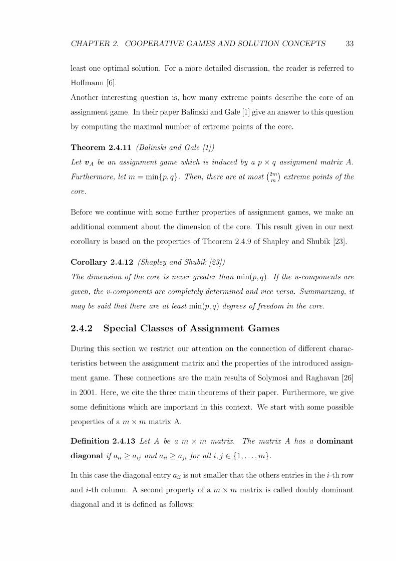
Theorem 2.4.11 (Balinski and Gale [1])
Let vA be an assignment game which is induced by a p × q assignment matrix A.
Furthermore, let m = min{p, q}. Then, there are at most(
2m
m
)
extreme points of the
core.
Before we continue with some further properties of assignment games, we make an
additional comment about the dimension of the core. This result given in our next
corollary is based on the properties of Theorem 2.4.9 of Shapley and Shubik [23].
Corollary 2.4.12 (Shapley and Shubik [23])
The dimension of the core is never greater than min(p, q). If the u-components are
given, the v-components are completely determined and vice versa. Summarizing, it
may be said that there are at least min(p, q) degrees of freedom in the core.
2.4.2 Special Classes of Assignment Games
During this section we restrict our attention on the connection of different charac-
teristics between the assignment matrix and the properties of the introduced assign-
ment game. These connections are the main results of Solymosi and Raghavan [26]
in 2001. Here, we cite the three main theorems of their paper. Furthermore, we give
some definitions which are important in this context. We start with some possible
properties of a m × m matrix A.
Definition 2.4.13 Let A be a m × m matrix. The matrix A has a dominant
diagonal if aii ≥ aij and aii ≥ aji for all i, j ∈ {1, . . . , m}.
In this case the diagonal entry aii is not smaller that the others entries in the i-th row
and i-th column. A second property of a m × m matrix is called doubly dominant
diagonal and it is defined as follows:
CHAPTER 2. COOPERATIVE GAMES AND SOLUTION CONCEPTS 34
Definition 2.4.14 Let A be a m × m matrix. The matrix A has a doubly domi-
nant diagonal if aii + akj ≥ aij + aki for all i, j, k ∈ {1, . . . , m}.
The two above properties are independent if m is bigger or equal than three. This
means that, a matrix can have a dominant diagonal but not a doubly dominant
diagonal and vice versa. In the next example we consider two matrices such that
one has only a dominant diagonal and the other one has only a doubly dominant
diagonal.
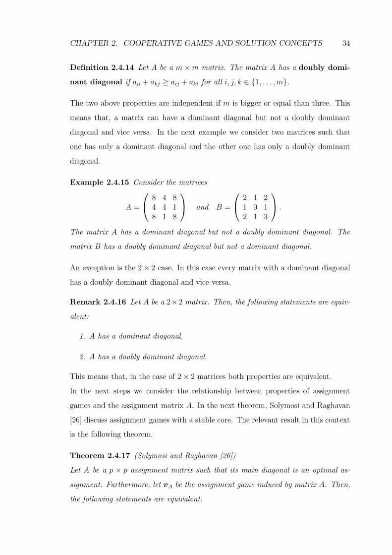
Example 2.4.15 Consider the matrices
A =
8 4 84 4 18 1 8
and B =
2 1 21 0 12 1 3
.
The matrix A has a dominant diagonal but not a doubly dominant diagonal. The
matrix B has a doubly dominant diagonal but not a dominant diagonal.
An exception is the 2 × 2 case. In this case every matrix with a dominant diagonal
has a doubly dominant diagonal and vice versa.
Remark 2.4.16 Let A be a 2×2 matrix. Then, the following statements are equiv-
alent:
1. A has a dominant diagonal,
2. A has a doubly dominant diagonal.
This means that, in the case of 2 × 2 matrices both properties are equivalent.
In the next steps we consider the relationship between properties of assignment
games and the assignment matrix A. In the next theorem, Solymosi and Raghavan
[26] discuss assignment games with a stable core. The relevant result in this context
is the following theorem.
Theorem 2.4.17 (Solymosi and Raghavan [26])
Let A be a p × p assignment matrix such that its main diagonal is an optimal as-
signment. Furthermore, let vA be the assignment game induced by matrix A. Then,
the following statements are equivalent:
CHAPTER 2. COOPERATIVE GAMES AND SOLUTION CONCEPTS 35
1. C(vA) is stable,
2. A has a dominant diagonal.
Thus, with the aid of this theorem, it is very simple to check whether an assignment
game has a stable core or not.
In a second step, we consider exact assignment games. As in the case of assignment
games with a stable core, Solymosi and Raghavan [26] have found some conditions
on the assignment matrix. Furthermore, the authors proved that an assignment
game is exact if and only if the assignment game has a large core. The results are
summarized in the next theorem.
Theorem 2.4.18 (Solymosi and Raghavan [26])
Let A be a p × p assignment matrix such that its main diagonal is an optimal as-
signment. Furthermore, let vA be the assignment game induced by matrix A. Then,
the following statements are equivalent:
1. vA is exact,
2. C(vA) is large,
3. A has a dominant and a doubly dominant diagonal.
This theorem permits the possibility to check if an assignment game is exact or not.
In particular, this theorem implies that exact assignment games have a stable core.
Before we are able to present convex assignment games, we need a further definition
of m × m matrices.
Definition 2.4.19 Let A be a m×m matrix. The matrix A is a diagonal matrix
if aij = 0 for all i, j ∈ {1, . . . , m}, i 6= j.
A diagonal matrix is the most restrictive property in the context of m×m matrices.
By definition a diagonal matrix has a dominant and a doubly dominant diagonal.
The next theorem treats convex assignment games. Solymosi and Raghavan [26]
showed that in this case the assignment matrix has a very special structure such
that it is very simple to identify these games.
CHAPTER 2. COOPERATIVE GAMES AND SOLUTION CONCEPTS 36
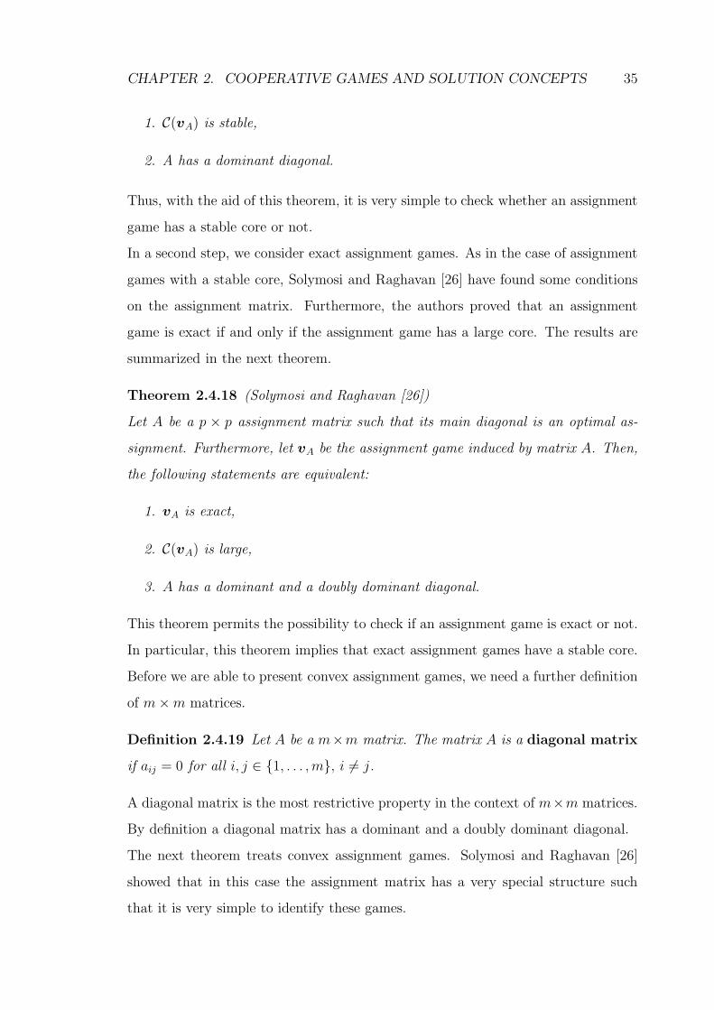
Theorem 2.4.20 (Solymosi and Raghavan [26])
Let A be a p × p assignment matrix such that its main diagonal is an optimal as-
signment. Furthermore, let vA be the assignment game induced by matrix A. Then,
the following statements are equivalent:
1. vA is convex,
2. A is a diagonal matrix.
Since a diagonal matrix has a dominant and a doubly dominant diagonal, one im-
mediately sees that convex assignment games are exact and have a stable core.
Furthermore, we note that convexness is invariant under adding nullplayers such
that we have the following result:
Corollary 2.4.21 Let A be a p× q assignment matrix such that the diagonal is an
optimal assignment. Then, the following statements are equivalent:
1. vA is convex,
2. aij′ = 0 ∀(i, j′) ∈ P × Q, (i, j′) /∈ D.
2.4.3 Modified Nucleolus of Assignment Games
In this section we are looking at the relationship between the core, the modified
least core of an assignment game and the least core of the dual assignment game.
These relationships are very useful since the modified nucleolus is an element of the
modified least core. If we find some results in this case, we can restrict our research
of the modiclus in some special cases on easier problems. In the next theorem,
Sudholter [31] proves that the modiclus of an assignment game is an element of the
least core of the dual game.
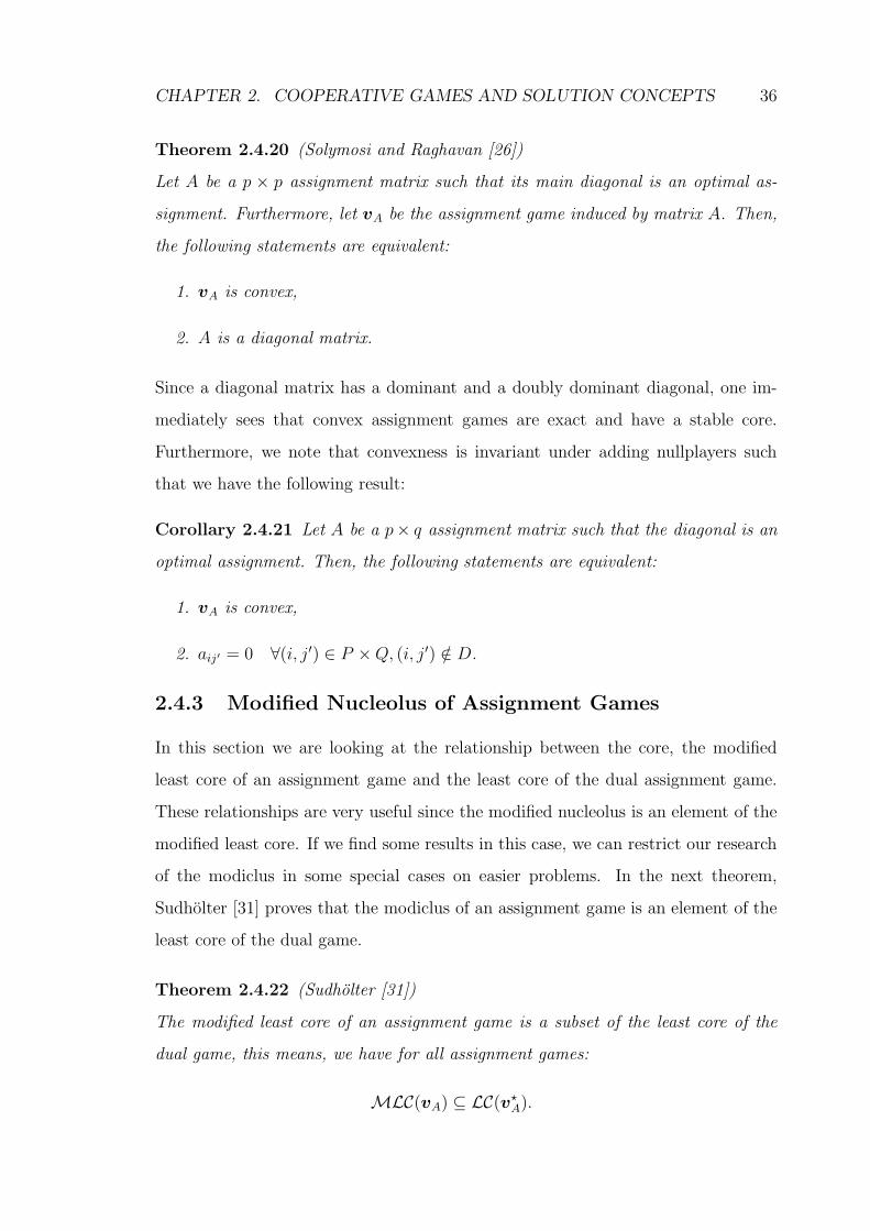
Theorem 2.4.22 (Sudholter [31])
The modified least core of an assignment game is a subset of the least core of the
dual game, this means, we have for all assignment games:
MLC(vA) ⊆ LC(v?A).
CHAPTER 2. COOPERATIVE GAMES AND SOLUTION CONCEPTS 37
Thus, the least core of the dual assignment game is an important set in the context
of the modified nucleolus of assignment games because the modified nucleolus is
an element of the modified least core. In the case of an assignment matrix with a
dominant diagonal, the modified nucleolus of the induced assignment game is also
an element of the core. This result is due to the following theorem of Raghavan and
Sudholter [12].
Theorem 2.4.23 (Raghavan and Sudholter [12])
If vA is an assignment game with a stable core, then the modified least core is a
subset of the core. Thus, we have for all assignment games with a stable core
MLC(vA) ⊆ C(vA).
This means that, the modiclus of an assignment game is an element of the least core
of the dual game and of the core, if it is stable. In particular we have in this case:
Ψ(vA) ∈ C(vA) ∩ LC(v?A) 6= ∅.
We conclude that Theorem 2.4.22 and Theorem 2.4.23 motivate a more detailed
discussion of the core and the least core of the dual assignment game.
2.5 Strong Nullplayer Property
In this section we are looking at some solution concepts which satisfy the strong
nullplayer property. With the aid of this property we can restrict our attention in
the next chapters on assignment games which are induced by a p × p assignment
matrix. In the case of assignment games with an unequal number of P and Q players
this property allows us to add some nullplayers.
When we define the strong nullplayer property, we look at two games such that the
first game is induced by the second one by adding a nullplayer. With the aid of
these two games, we are able to define this property.
Definition 2.5.1 Let (I,P(I), v) be a game and let I = I ∪ {n}. Consider the
game (I,P(I), v) which is defined by
v(S) = v(I ∩ S) ∀S ∈ P(I).
CHAPTER 2. COOPERATIVE GAMES AND SOLUTION CONCEPTS 38
A solution concept δ satisfies the strong nullplayer property if
δ(v) ={
x ∈ Rn+1 | xI ∈ δ(v), xn = 0}
(2.2)
holds true.
The strong nullplayer property implies that any nullplayer i ∈ I gets the payoff zero.
Additionally, the solution δ(v) of game v arises from the solution δ(v) of game v
by adding a zero coordinate for the nullplayer to any element of the solution δ(v).
Since the following chapter is about the Shapley value and the core of assignment
games, it is useful to check that these solution concepts satisfy the strong nullplayer
property. Thus, our next results are a preparation of the next chapter. In our first
lemma, we show that the core satisfies the strong nullplayer property.
Lemma 2.5.2 The core satisfies the strong nullplayer property.
Proof.
We show the equality (2.2) in two steps.
“ ⊇ “
Let x ∈ {x ∈ Rn+1 | xI ∈ C(v), xn = 0}.
Since xI ∈ C(v), we can conclude that
x(S) ≥ v(S ∩ I) = v(S) ∀S ⊆ I .
Knowing that
v(I) = v(I),
one immediately sees that x(I) = v(I), such that we can conclude that x ∈ C(v).
“ ⊆ “
Now, let x ∈ C(v) = {x ∈ Rn+1 | x(I) = v(I), x(S) ≥ v(S) ∀S ∈ P(I)}.
By definition it follows immediately that
x(I) ≥ x(I) ≥ v(I) = v(I).
Thus, all inequalities are equalities, and in view of x(I) = x(I), it is clear that
xn = 0. Since v(S) = v(S) for all S ∈ P(I), we can conclude that xI ∈ C(v). 2

CHAPTER 2. COOPERATIVE GAMES AND SOLUTION CONCEPTS 39
Thus, if we look at the core, it is possible to add nullplayers without changing the
results.
Another solution concept which satisfies the strong nullplayer property is the Shapley
value. This result is topic of the following lemma.
Lemma 2.5.3 The Shapley value satisfies the strong nullplayer property.
Proof.
In order to prove the strong nullplayer property, we have to show that
φi(v) = φi(v) ∀i ∈ {1, . . . , n}, (2.3)
φn(v) = 0. (2.4)
Note, that if the equality (2.3) holds, equality (2.4) follows immediately by the
definition of the Shapley value. Now, let i ∈ {1, . . . n} and let S ⊆ I \ {i}. For each
S = {i1, . . . , is} ⊆ I \ {i} we define two subsets Ks, Ls ⊆ I \ {i} by
1. Ks = K = S = {i1 . . . , is}
2. Ls = L = S ∪ {n} = {i1 . . . , is, n}.
By definition of the game v, we have for every sets S ⊆ I \ {i} and the induced
coalitions Ks = K and Ls = L the following result:
v(K ∪ {i}) = v(L ∪ {i}) = v(S ∪ {i}) and v(K) = v(L) = v(S).
We have finished the proof, if we can show that
γ(s)(v(S ∪ {i} − v(S)) = γ(k)(v(K ∪ {i}) − v(K)) + γ(l)(v(L ∪ {i}) − v(L)).
This equality holds true if and only if
γ(s) = γ(k) + γ(l)
holds true. To show this equality, we denote the number of players of coalition K
and S with t = |K| = |S|.
CHAPTER 2. COOPERATIVE GAMES AND SOLUTION CONCEPTS 40
Then, we have:
γ(s) =1
n
1(
n−1t
)
=t! · (n − 1 − t)!
n · (n − 1)!
=t! · (n + 1) · (n − 1 − t)!
(n + 1)!
=t! · (n − 1 − t)![(n − t) + (t + 1)]
(n + 1)!
=t! · (n − t)! + (t + 1)! · (n − t − 1)!
(n + 1)!
=1
(n + 1)
1(
n
t
) +1
(n + 1)
1(
n
t+1
)
= γ(k) + γ(l)
This equality proves our lemma. 2
Thus, we have shown that the Shapley value satisfies the strong nullplayer property.
In this case results about the Shapley value are independent of nullplayers.
For reasons of completeness let us remark that Sudholter proved in his papers [29,
30] that the modiclus also satisfies the strong nullplayer property.
Since we have seen that there exists different solution concepts which satisfy the
strong nullplayer property, we will see that there exists solution concepts which do
not satisfy this property.
Remark 2.5.4 Typically, the least core does not satisfy the strong nullplayer prop-
erty.
To see this, we look at an example of a cooperative game such that its least core
does not satisfy the strong nullplayer property.
Example 2.5.5 Consider the following game (I,P(I), v) which is defined by:
I = {1, 2, 3},
v(I) = 1,
v({1, 2}) = v({1, 3}) =3
4,
v(S) = 0 ∀S ∈ P(I).
CHAPTER 2. COOPERATIVE GAMES AND SOLUTION CONCEPTS 41
Let I = {1, 2, 3, 4} and let (I ,P(I), v) be a game defined by
v(S) = v(I ∩ S) for all S ∈ P(I).
In this case we have
(
3
4,1
8,1
8
)
∈ LC(v) = C− 1
8
(v)
and
(
3
4,1
8,1
8, 0
)
∈ LC(v) = C0(v).
But, there exists an element
(1, 0, 0, 0) ∈ LC(v) = C0(v)
with
(1, 0, 0) /∈ LC(v).
Thus, the least core does not satisfy the strong nullplayer property.
As we will see in a later theorem, the least core of the dual assignment game satisfies
the strong nullplayer property. This is possible because, as we will see later, the least
core of these games has more structure.
Chapter 3
The Shapley Value and the Core
3.1 Introduction
Both, the Shapley value and the core are well-known solution concepts in cooper-
ative game theory. Since these two concepts are characterized differently, it is not
surprising that the Shapley value of a game need not be an element of the core,
even if the core is non-empty. But there exist subclasses of balanced games such
that the Shapley value is in the core. One of the most important subclass is the
subclass of convex games. The main focus of this chapter is the well-studied subclass
of assignment games. Until now, very little is known about their Shapley value. If
one considers assignment games with an unequal numbers of P and Q players, the
Shapley value cannot be in the core. To see this, note that the players who are
not matched in an optimal assignment of the grand coalition get nothing in any
core allocation. But the expected payoff of every non-nullplayer is however posi-
tive. During this chapter we are looking for some necessary conditions so that the
Shapley value is an element of the core. Therefore, we will start in the first section
with partially average convex games and with partially average convex assignment
games. In the second section we concentrate on some properties of exact assignment
games. The main result of this section is the connection between the Shapley value
and the core in the case of exact assignment games. Next, we look at an example of
a game with a large core such that the Shapley value is not an element of the core.
In the last step we will see that there exist non-exact assignment games such that
the Shapley value is in the core.
42
CHAPTER 3. THE SHAPLEY VALUE AND THE CORE 43
3.2 Partially Average Convex Games
In this section we concentrate on partially average convex games, which include the
class of convex games. In order to define these games, we have a look at the following
function.
Definition 3.2.1 Let (I,P, v) be a cooperative game. A function
gv : P × P → R
is defined by
gv(A, B) = v(A ∪ B) − v(A) − v(B) ∀A, B ⊆ I, A ∩ B = ∅.
Note, that by definition, we have for all A, B ⊆ I, A∩B = ∅ the following equality:
gv(A, B) = gv(B, A).
That means, we have a kind of symmetry. The value gv(A, B) can be interpreted
as gain (or loss) if two disjoint coalitions cooperate instead of stayed in the two
coalitions A and B. With the aid of this function, we can define our next class of
cooperative games, which dues to Inarra and Usategui [8] in 1993.
Definition 3.2.2 (Inarra and Usategui [8])
A cooperative game v is partially average convex if(
b
r
)−1∑
R⊆B,|R|=r
gv(A, R) ≥
(
b
c
)−1∑
C⊂B,|C|=c
gv(A, B \ C)
for all A, B ⊆ I, B ⊆ I \ A and for any r and c such that
r >ab
n − b> b − c if A ∪ B ⊂ I, and
r = b > c if A ∪ B = I.
Note, that every convex game is partially average convex. Furthermore, by Theorem
5 of Inarra and Usategui [8] the Shapley value of partially average convex games is
an element of the core.
Theorem 3.2.3 (Inarra and Usategui [8])
The Shapley value of a partially average convex game is in the core.
In particular, we know that the core of these games is non-empty.
CHAPTER 3. THE SHAPLEY VALUE AND THE CORE 44
3.2.1 Partially Average Convex Assignment Games
In this section we are looking at partially average convex assignment games. We
will see that in the case of assignment games Theorem 3.2.3 is no gain, because an
assignment game vA is convex if and only if it is partially average convex. This
result is subject of the following lemma of Hoffmann and Sudholter [7] in 2007.
Lemma 3.2.4 (Hoffmann and Sudholter [7])
Let A be a non-negative p× p assignment matrix such that the main diagonal is an
optimal assignment. If p ≥ 3 holds true, the following statements are equivalent:
1. vA is partially average convex,
2. vA is convex.
Proof.
“1. ⇒ 2.“
Let vA = v be a partially average convex assignment game and let i, j ∈ P such
that i 6= j. Furthermore, let A = P ∪ {j′} and B = {i, i′}. For r = b = 2 and c = 1
we have
r = 2 >2p
2p − 2=
ab
n − 2> 1 = b − c
and(
b
r
)−1∑
R⊆B,|R|=r
gv(A, R) = 0,
(
b
c
)−1∑
C⊂B,|C|=c
gv(A, B \ C) =1
2max
k∈P\{i,j}aki′ .
Thus,
0 ≥1
2max
k∈P\{i,j}aki′
holds true if A is a diagonal matrix. By Theorem 2.4.17 of Solymosi and Raghavan
[26] the induced assignment game vA is a convex game.
“2. ⇒ 1.“
By Inarra and Usategui [8], every convex game is partially average convex. 2
Thus, we have seen that an assignment game which is induced by a p × p, p ≥ 3,
assignment matrix is convex if and only if it is partially average convex.
CHAPTER 3. THE SHAPLEY VALUE AND THE CORE 45
3.3 The Shapley Value as an Element of the Core
In this section we concentrate on some aspects which imply that the Shapley value
is an element of the core. Inarra and Usategui [8] have found an interesting result
in this context. In order to cite their result, we have to define a real-valued function
on the set of coalitions P.
Definition 3.3.1 (Inarra and Usategui [8])
Let (I,P, v) be a cooperative game. A function
αT : P → R
is defined by
αT (S) =|S ∩ T |n − st
n − s= s
(
|S ∩ T |
s−
|T \ S|
n − s
)
∀S, T ⊆ I, S 6= I
αT (I) = t ∀T ⊆ I.
Note, that αT (S) may be negative even if S ∩ T 6= ∅.
In the next theorem of Inarra and Usategui, we will see that there exists a property
which is equivalent to the fact, that the Shapley value is an element of the core.
Theorem 3.3.2 (Inarra and Usategui [8])
Let (I,P, v) a cooperative game. Then, the following statements are equivalent:
1. Φ(v) ∈ C(v),
2.∑
∅6=S⊆I γ(S) αT (S) gv(S \ T, S ∩ T ) ≥ 0 ∀T ⊂ I, T 6= ∅.
Thus, we have a possibility to check, if the Shapley value is in the core or not. In the
following sections, we are looking for other possibilities to characterize assignment
games such that the Shapley Value is in the core. We will see that in the case of
assignment games, we do not have to use the above results.
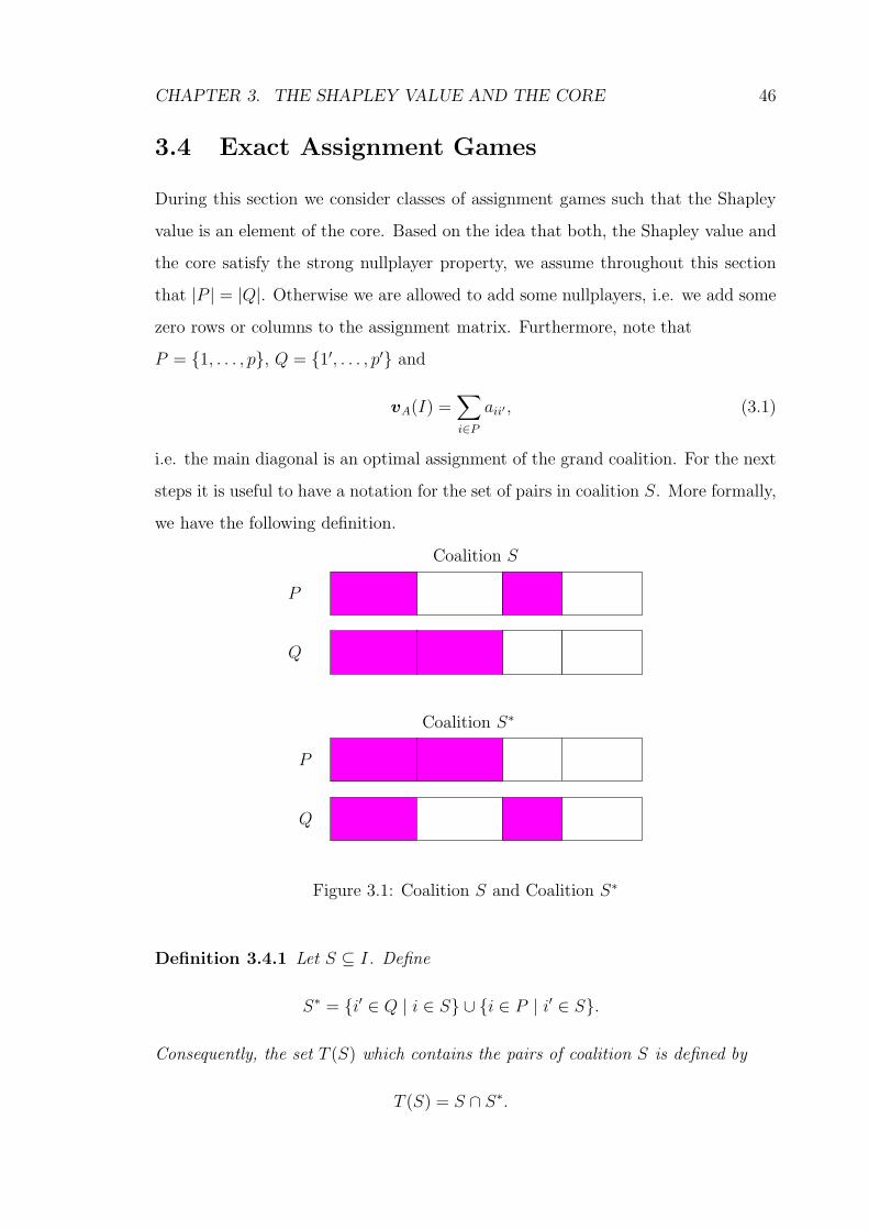
CHAPTER 3. THE SHAPLEY VALUE AND THE CORE 46
3.4 Exact Assignment Games
During this section we consider classes of assignment games such that the Shapley
value is an element of the core. Based on the idea that both, the Shapley value and
the core satisfy the strong nullplayer property, we assume throughout this section
that |P | = |Q|. Otherwise we are allowed to add some nullplayers, i.e. we add some
zero rows or columns to the assignment matrix. Furthermore, note that
P = {1, . . . , p}, Q = {1′, . . . , p′} and
vA(I) =∑
i∈P
aii′ , (3.1)
i.e. the main diagonal is an optimal assignment of the grand coalition. For the next
steps it is useful to have a notation for the set of pairs in coalition S. More formally,
we have the following definition.
Coalition S
Coalition S∗
P
P
Q
Q
Figure 3.1: Coalition S and Coalition S∗
Definition 3.4.1 Let S ⊆ I. Define
S∗ = {i′ ∈ Q | i ∈ S} ∪ {i ∈ P | i′ ∈ S}.
Consequently, the set T (S) which contains the pairs of coalition S is defined by
T (S) = S ∩ S∗.
CHAPTER 3. THE SHAPLEY VALUE AND THE CORE 47
In Figure 3.1 we see a geometric view of the sets S and S∗.
Note, that S∗ is the set of all partners of players in S according to an optimal
assignment of I. Furthermore, for all S ⊆ I we have |S∗| = |S| and (S∗)∗ = S. In
our next remark we consider the worth of the set T (S) of an assignment game.
Remark 3.4.2 Let vA be an assignment game. By Definition 2.4.3 and (3.1), we
have for all S ⊆ I the following equality:
vA(T (S)) = vA(S ∩ S∗) =∑
i∈P∩S∩S∗
aii′ . (3.2)
Thus, the worth of coalitions, which only contains pairs, is equal to the sum of the
corresponding diagonal elements.
Our next lemma characterizes a partition of the payoff vA(S) of an exact assignment
game. We will see that in the case of exact assignment games we can compute this
value by adding the payoffs vA(T (S)) and vA(S \ T (S)). With the aid of this
partition, it is possible to prove our main Theorem 3.4.4.
Lemma 3.4.3 (Hoffmann and Sudholter [7])
Let vA be an assignment game such that the main diagonal of the assignment matrix
is an optimal assignment. Then, the following statements are equivalent:
1. vA(S) satisfies
vA(S) = vA(T (S)) + vA(S \ T (S)) ∀S ⊆ I. (3.3)
2. vA is exact.
Proof.
We prove the above statement in two steps.
“1. ⇒ 2.“
Assume that (3.3) is satisfied. Let i ∈ P and j, k ∈ P \ {i}. By Definition 2.4.3, we
have:
aii′ + ajk′ = vA({i, j, i′, k′}) ≥ aik′ + aji′,
aii′ = vA({i, j, i′}) ≥ aji′,
aii′ = vA({i, i′, k′}) ≥ aik′.
CHAPTER 3. THE SHAPLEY VALUE AND THE CORE 48
Hence, the assignment matrix A has a doubly dominant and a dominant diagonal
such that the induced assignment game vA is exact.
“2. ⇒ 1.“
Let vA be an exact assignment game such that the assignment matrix A has a
dominant and doubly dominant diagonal. Let S ⊆ I and define T = T (S) = S∩S∗.
We shall prove (3.3) by induction on |T | = t. Indeed, if t = 0, then T = ∅ and (3.3)
is true. Assume now that t > 0. Let b be an optimal assignment for S and let i ∈ T .
By the inductive hypothesis and (3.2) it remains to show that
vA(S) ≤ aii′ + vA(S \ {i, i′}).
If (i, i′) ∈ b, then the proof is complete. Hence, we may assume that (i, i′) /∈ b. The
following three cases may occur.
Case 1:
There exists j′ ∈ S ∩ Q, j 6= i, such that (i, j′) ∈ b and i′ is not matched in b, that
is,
{(j, i′) | j ∈ P} ∩ b = ∅.
As the assignment matrix A has a dominant diagonal,
vA(S) = vA(S \ {i, i′, j′}) + aij′ ≤ vA(S \ {i, i′, j′}) + aii′ ≤ vA(S \ {i, i′}) + aii′ .
Case 2:
The case where there exists j ∈ S∩P, j 6= i, such that (j, i′) ∈ b and i is not matched
in b, that is,
{(i, j′) | j ∈ P} ∩ b = ∅,
may be treated analogously to (1).
Case 3:
If (i, k′), (j, i′) ∈ b for some j, k ∈ P \ {i}, then we have
vA(S) = vA(S \ {i, i′, j, k′}) + aik′ + aji′
≤ vA(S \ {i, i′, j, k′}) + aii′ + ajk′
≤ vA(S \ {i, i′}) + aii′ ,
CHAPTER 3. THE SHAPLEY VALUE AND THE CORE 49
because A has a doubly dominant diagonal. 2
Note, that Lemma 3.4.3 gives a further possible description of exact assignment
games. With the aid of this result, it is possible to prove our main result in the next
section.
3.4.1 The Shapley Value of Exact Assignment Games
In the previous sections of this chapter we looked for characteristics of partially
average convex and of exact assignment games. The problem we now wish to study
is the connection between the Shapley value and the core of exact assignment games.
The following theorem is the main result of Hoffmann and Sudholter [7] in 2007.
This result can be proven in a direct way with the aid of Theorem 2.4.9 and Lemma
3.4.3. The results of Inarra and Usategui [8] are not used in the proof.
Theorem 3.4.4 (Hoffmann and Sudholter [7])
Let vA be an assignment game induced by the p × p assignment matrix A. Further-
more, let the main diagonal of the matrix A be an optimal assignment. In the case
that vA is an exact assignment game, we have
Φ(vA) ∈ C(vA).
Proof.
Let Φ(vA) = x = (u, v). By Definition 2.3.37, we have Φ(vA) ≥ 0. In view of
Theorem 2.4.9 and (3.1) it suffices to show that
ui + vi′ = aii′ for all i ∈ P, (3.4)
ui + vj′ ≥ aij′ for all i, j ∈ P. (3.5)
Note, that (3.4) implies that x(I) = vA(I) =∑
i∈P aii′ . Now, let i ∈ P .
Step 1:
We shall show that for i ∈ P we have ui + vi′ = aii′ . Let |I| = n and note that, by
the definition of γ(·), we have
γ(s) = γ(n − s − 1) for all s = 0, . . . , n − 1. (3.6)
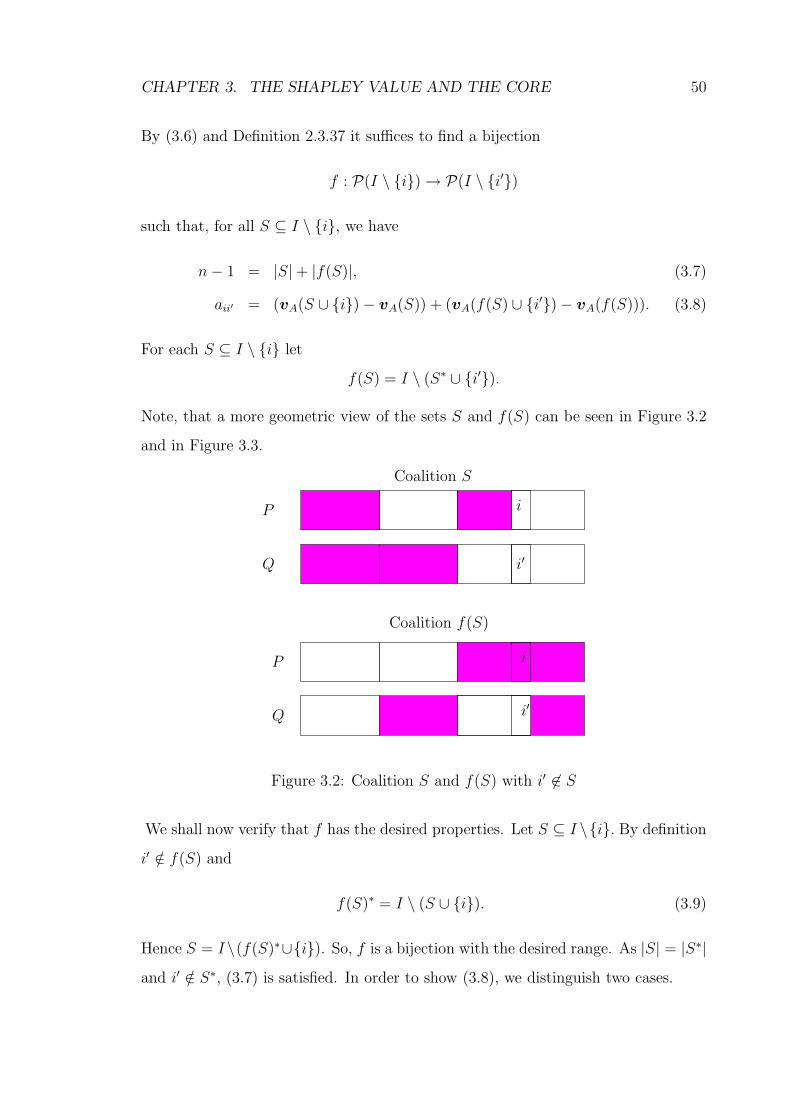
CHAPTER 3. THE SHAPLEY VALUE AND THE CORE 50
By (3.6) and Definition 2.3.37 it suffices to find a bijection
f : P(I \ {i}) → P(I \ {i′})
such that, for all S ⊆ I \ {i}, we have
n − 1 = |S| + |f(S)|, (3.7)
aii′ = (vA(S ∪ {i}) − vA(S)) + (vA(f(S) ∪ {i′}) − vA(f(S))). (3.8)
For each S ⊆ I \ {i} let
f(S) = I \ (S∗ ∪ {i′}).
Note, that a more geometric view of the sets S and f(S) can be seen in Figure 3.2
and in Figure 3.3.
Coalition f(S)
P
P
Q
Q
i
i
i′
i′
Coalition S
Figure 3.2: Coalition S and f(S) with i′ 6∈ S
We shall now verify that f has the desired properties. Let S ⊆ I \{i}. By definition
i′ /∈ f(S) and
f(S)∗ = I \ (S ∪ {i}). (3.9)
Hence S = I \(f(S)∗∪{i}). So, f is a bijection with the desired range. As |S| = |S∗|
and i′ /∈ S∗, (3.7) is satisfied. In order to show (3.8), we distinguish two cases.
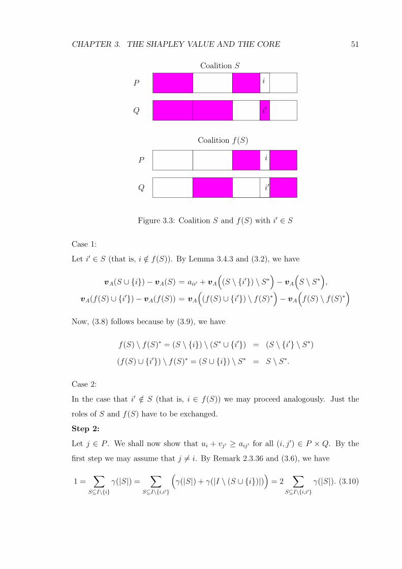
CHAPTER 3. THE SHAPLEY VALUE AND THE CORE 51
Coalition f(S)
P
P
Q
Q
i
i
i′
i′
Coalition S
Figure 3.3: Coalition S and f(S) with i′ ∈ S
Case 1:
Let i′ ∈ S (that is, i /∈ f(S)). By Lemma 3.4.3 and (3.2), we have
vA(S ∪ {i}) − vA(S) = aii′ + vA
(
(S \ {i′}) \ S∗)
− vA
(
S \ S∗)
,
vA(f(S) ∪ {i′}) − vA(f(S)) = vA
(
(f(S) ∪ {i′}) \ f(S)∗)
− vA
(
f(S) \ f(S)∗)
Now, (3.8) follows because by (3.9), we have
f(S) \ f(S)∗ = (S \ {i}) \ (S∗ ∪ {i′}) = (S \ {i′} \ S∗)
(f(S) ∪ {i′}) \ f(S)∗ = (S ∪ {i}) \ S∗ = S \ S∗.
Case 2:
In the case that i′ /∈ S (that is, i ∈ f(S)) we may proceed analogously. Just the
roles of S and f(S) have to be exchanged.
Step 2:
Let j ∈ P . We shall now show that ui + vj′ ≥ aij′ for all (i, j′) ∈ P × Q. By the
first step we may assume that j 6= i. By Remark 2.3.36 and (3.6), we have
1 =∑
S⊆I\{i}
γ(|S|) =∑
S⊆I\{i,i′}
(
γ(|S|) + γ(|I \ (S ∪ {i})|))
= 2∑
S⊆I\{i,i′}
γ(|S|). (3.10)
CHAPTER 3. THE SHAPLEY VALUE AND THE CORE 52
Let R = P(I \ {i, i′, j, j′}). By (3.6) applied to any R ∪ {i′}, R ∈ R and by (3.10),
1 = 2∑
R⊆I\{i,i′,j,j′}
(
γ(|R|) + γ(|R ∪ {i′}|) + γ(|R ∪ {j}|) + γ(|R ∪ {j′}|))
=∑
R⊆I\{i,i′,j,j′}
(
2γ(|R|) + 6γ(|R| + 1))
. (3.11)
For R ⊆ I, let r = |R|. By (3.11) it suffices to show that for all R ∈ R there are
c(R), d(R) ∈ R, such that
ui + vj′ =∑
R∈R(c(R)γ(r) + d(R)γ(r + 1)), (3.12)
c(R) ≥ 2aij′ and d(R) ≥ 6aij′. (3.13)
By Definition 2.3.37 and using s = |S|, we have
ui + vj′ =∑
S⊆I\{i,j′}
(
γ(s)(
vA(S ∪ {i}) + vA(S ∪ {j′}) − 2vA(S))
+ (3.14)
γ(s + 1)(
2vA(S ∪ {i, j′}) − vA(S ∪ {j′}) − vA(S ∪ {i})))
.
To every R ∈ R we assign three coalitions defined by
fj(R) = (I \ R∗) \ {j},
fi′(R) = (I \ R∗) \ {i′},
fij′(R) = (I \ R∗) \ {i, j′}.
Note, that fj(·), fi′(·) and fij′(·) are injective mappings in R. Observe that for any
S ⊆ I \ {i, j′} there exists a unique R ∈ R such that S coincides with one of the
sets R, R ∪ {j}, R ∪ {i′} and fij′(R). Similarly, note that there exists a unique
R ∈ R such that S ∪ {i, j′} coincides with one of the sets I \ R∗, fj(R), fi′(R) and
R ∪ {i, j′}. Let R ∈ R and let
c(R) = vA(R ∪ {i}) + vA(R ∪ {j′}) − 2vA(R) + 2vA(I \ R∗)
−vA((I \ R∗) \ {i}) − vA((I \ R∗) \ {j′},
CHAPTER 3. THE SHAPLEY VALUE AND THE CORE 53
let
dj(R) = vA(R ∪ {i, j}) + vA(R ∪ {j, j′}) − 2vA(R ∪ {j})
+2vA(fj(R)) − vA(fj(R) \ {i}) − vA(fj(R) \ {j′}),
di′(R) = vA(R ∪ {i, i′}) + vA(R ∪ {i′, j′}) − 2vA(R ∪ {i′})
+2vA(fi′(R)) − vA(fi′(R) \ {i}) − vA(fi′(R) \ {j′}),
dij′(R) = vA(fij′(R) ∪ {i}) + vA(fij′(R) ∪ {j′}) − 2vA(fij′(R))
+2vA(R ∪ {i, j′}) − vA(R ∪ {j′}) − vA(R ∪ {i}),
and put d(R) = dj(R)+di′(R)+dij′(R). Thus, (3.12) is implied by (3.14) and (3.6).
Let R = R \ R∗. Lemma 3.4.3 together with (3.2) yield
c(R) = aii′ + ajj′ + vA(R ∪ {i}) − vA(R ∪ {i′}) − vA(R ∪ {j}) + vA(R ∪ {j′}),
dj(R) = aii′ + ajj′ − 2vA(R ∪ {j}) + 2vA(R ∪ {j′}) + vA(R ∪ {i, j})
−vA(R ∪ {i′, j′}),
di′(R) = aii′ + ajj′ + 2vA(R ∪ {i}) − 2vA(R ∪ {i′}) − vA(R ∪ {i, j})
+vA(R ∪ {i′, j′}),
dij′(R) = aii′ + ajj′ − vA(R ∪ {i}) + vA(R ∪ {i′}) + vA(R ∪ {j}) − vA(R ∪ {j′})
+2vA(R ∪ {i, j′}) − 2vA(R ∪ {i′, j}).
We conclude that
d(R) = 3aii′ + 3ajj′ + vA(R ∪ {i}) − vA(R ∪ {i′}) − vA(R ∪ {j})
+vA(R ∪ {j′}) + 2vA(R ∪ {i, j′}) − 2vA(R ∪ {i′, j}).
Therefore, in order to verify (3.13) it suffices to prove that
aij′ ≤ aii′ + vA(R ∪ {j′}) − vA(R ∪ {i′}), (3.15)
aij′ ≤ ajj′ + vA(R ∪ {i}) − vA(R ∪ {j}), (3.16)
2aij′ ≤ aii′ + ajj′ + vA(R ∪ {i, j′}) − vA(R ∪ {j, i′}). (3.17)
In order to show (3.15) we distinguish two cases. If i′ is not matched in an optimal
assignment of R∪ {i′}, that is, if vA(R∪ {i′}) = vA(R), then the desired inequality
CHAPTER 3. THE SHAPLEY VALUE AND THE CORE 54
is immediately implied, because A has a dominant diagonal. If i′ is matched to some
k ∈ P ∩ R in an optimal assignment, that is, if vA(R ∪ {i′}) = aki′ + vA(R \ {k}),
then vA(R ∪ {j′}) ≥ akj′ + vA(R \ {k}) implies that
aii′ + vA(R ∪ {j′}) − vA(R ∪ {i′}) ≥ aii′ + akj′ − aki′
and, so (3.15) is valid, because A has a doubly dominant diagonal. In a completely
analogous way we may show (3.16).
In order to prove (3.17), put
β = aii′ + ajj′ + vA(R ∪ {i, j′}) − vA(R ∪ {j, i′}).
Let b ∈ B(P ∩ (R ∪ {j}), Q ∩ (R ∪ {i′})) be an optimal assignment for R ∪ {j, i′}.
Four cases may occur.
Case 1:
(j, i′) ∈ b. So, vA(R ∪ {j, i′}) = vA(R) + aji′. As vA(R ∪ {i, j′}) ≥ vA(R) + aij′, we
may conclude that
β ≥ aii′ + ajj′ + aij′ − aji′ ≥ 2aij′,
because A has a dominant diagonal.
Case 2:
There exists some ` ∈ P ∩ R such that (`, i′) ∈ b and j is not matched in b. Then,
vA(R ∪ {j, i′}) = a`i′ + vA(R \ {`}) and vA(R ∪ {i, j′}) ≥ a`j′ + vA(R \ {`}). So,
β ≥ aii′ + ajj′ + a`j′ − a`i′ ≥ ajj′ + aij′ + a`i′ − a`i′ ≥ 2aij′,
where the second inequality is true, because A has a doubly dominant diagonal, and
the third inequality holds, because A has a dominant diagonal and vA is superad-
ditive.
Case 3:
There exists k′ ∈ Q ∩ R such that (j, k′) ∈ b and i′ is not matched in b. Then,
vA(R ∪ {j, i′}) = ajk′ + vA(R \ {k′}), vA(R ∪ {i, j′}) ≥ aik′ + vA(R \ {k′}) and,
analogously to Case 2, we have
β ≥ aii′ + ajj′ + aik′ − ajk′ ≥ aii′ + ajk′ + aij′ − ajk′ ≥ 2aij′.
CHAPTER 3. THE SHAPLEY VALUE AND THE CORE 55
Case 4:
There exist k′ ∈ Q ∩ R and ` ∈ P ∩ R such that (j, k′), (`, i′) ∈ b. Then,
vA(R ∪ {j, i′}) = ajk′ + a`i′ + vA(R \ {`, k′})
and
vA(R ∪ {i, j′}) ≥ aik′ + a`j′ + vA(R \ {`, k′}).
Applying the fact that A has a doubly dominant diagonal twice yields,
β ≥ aii′ + ajj′ + aik′ + a`j′ − ajk′ − a`i′
≥ aij′ + a`i′ + ajk′ + aij′ − ajk′ − a`i′
= 2aij′.
Thus, we have shown that the Shapley value of exact assignment games lies in the
core. 2
Before we consider cooperative games with a large core, we summarize by saying
that there exists a further class of games such that the Shapley value is an element
of the core. We have seen that convex games, partially average convex games and
exact assignment games are such games.
3.4.2 Games with a Large Core
In this section we introduce an example of an exact cooperative game with trans-
ferable utility (I,P, v) such that the core is large and does not contain the Shapley
value. Since assignment games are exact if and only if they have a large core, this
example completes our Theorem 3.4.4 because the example shows that the structure
of the assignment games is necessary for the above result. In the following example
we present a cooperative game with five players, which is defined with the aid of a
minimum of three non-negative additive functions.
Example 3.4.5 (Hoffmann and Sudholter [7])
Let I = {1, . . . , 5} and let λ1, λ2, λ3 ∈ A be given by
λ1 = (1, 1, 1, 0, 0), λ2 = (1, 1, 0, 1, 0), λ3 = (0, 0, 1, 1, 1).
CHAPTER 3. THE SHAPLEY VALUE AND THE CORE 56
We define a cooperative game (I,P, v) by
v(S) = minr=1,2,3
λr(S) ∀S ⊆ I.
In the next step we think about exactness and the Shapley value of this game. We
will see, that in the case of the above example, the Shapley value is an element of
the core. For more details, consider the following remark.
Remark 3.4.6 (Hoffmann and Sudholter [7])
Since λr(I) = 3 for all r = 1, 2, 3, we can conclude that the game (I,P, v) of
Example 3.4.5 is exact. By Definition 2.3.37, we have
Φ(v) = Φ =1
60(36, 36, 41, 41, 26).
In order to check that the Shapley value is not an element of the core, consider the
following inequality
v({2, 3, 4}) = 2 >118
60= Φ({2, 3, 4}),
such that we can conclude that
Φ(v) /∈ C(v).
In the last step, we are left to prove the following lemma in which we show that the
above game has a large core.
Lemma 3.4.7 (Hoffmann and Sudholter [7])
The game (I,P, v) of Example 3.4.5 has a large core.
Proof:
Let
X = {x ∈ A | x(S) ≥ v(S) for all S ⊆ I}.
Taking into account that v is monotonic, that 1 and 2 as well as 3 and 4 are
substitutes, and a careful inspection of the coalition function v yields that x ∈ X if
CHAPTER 3. THE SHAPLEY VALUE AND THE CORE 57
and only if
x ≥ 0; (3.18)
x3 + x4 ≥ 1; (3.19)
xi + xj ≥ 1 for all i ∈ {1, 2} and j ∈ {3, 4, 5}; (3.20)
xi + x3 + x4 ≥ 2 for all i ∈ {1, 2}. (3.21)
Note, that (3.20) and (3.21) imply x(I) ≥ 3 = v(I). Let x ∈ X and
Y = {y ∈ X | y ≤ x}.
Then, Y is a non-empty compact (convex polyhedral) set. As y 7→ y(I), y ∈ Y , is
continuous, there exists z ∈ Y such that z(I) ≤ y(I) for all y ∈ Y . It remains to
show that z(I) = v(I) = 3. By (3.18) one of the following 4 cases occurs.
Case 1:
z1 = 0. Then, by (3.20), zi ≥ 1 for all i = 3, 4, 5, and, by (3.18), z ≥ λ3. As λ3 ∈ X,
z = λ3 and the proof is complete.
Case 2:
The case z2 = 0 may be treated analogously.
Case 3:
z5 = 0. Then, (3.20) implies z1, z2 ≥ 1 and (3.19) implies that z3 + z4 ≥ 1. As z(I)
is minimal, z ≥ 0 implies that z3 + z4 = 1 = z1 = z2. Hence, z(I) = 3.
Case 4:
z1, z2, z5 > 0. Then, z1 = z2 ≤ 2 by minimality of z(I). In view of (3.19),
z1 = z2 ≤ 1. Again minimality implies that z1 + z5 = z2 + z5 = 1. By (3.21),
z3 + z4 ≥ 2− z1. So it remains to show that z3 + z4 = 2− z1. Assume the contrary.
As 3 and 4 are substitutes, we may assume that z3 ≥ z4. Then, z3 > 1 − z1
2. As
z1 ≤ 2, there exists ε ≥ 0 such that z3−ε ≥ 0, z1 +z3−ε ≥ 1 and z3 +z4−ε ≥ 2−z1
and a contradiction to the minimality of z(I) has been obtained. 2
Thus, we have found an example of an exact game with a large core, such that the
Shapley value is not an element of the core. This means, the special structure of
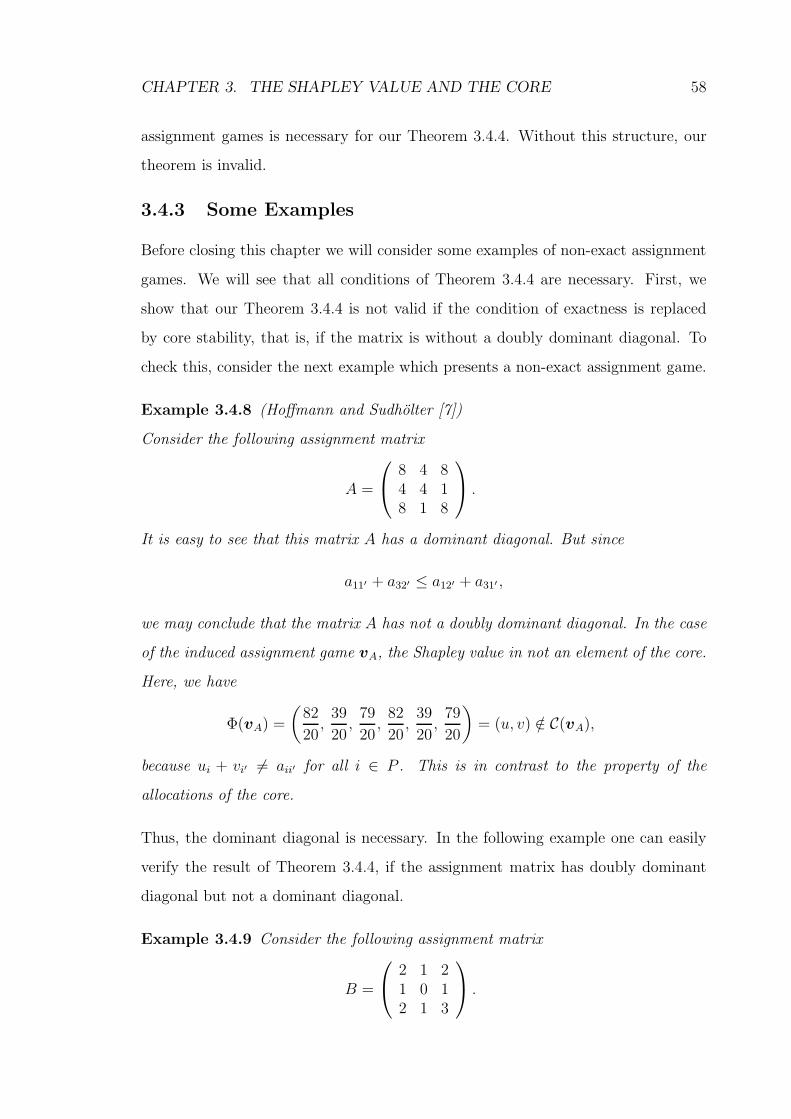
CHAPTER 3. THE SHAPLEY VALUE AND THE CORE 58
assignment games is necessary for our Theorem 3.4.4. Without this structure, our
theorem is invalid.
3.4.3 Some Examples
Before closing this chapter we will consider some examples of non-exact assignment
games. We will see that all conditions of Theorem 3.4.4 are necessary. First, we
show that our Theorem 3.4.4 is not valid if the condition of exactness is replaced
by core stability, that is, if the matrix is without a doubly dominant diagonal. To
check this, consider the next example which presents a non-exact assignment game.
Example 3.4.8 (Hoffmann and Sudholter [7])
Consider the following assignment matrix
A =
8 4 84 4 18 1 8
.
It is easy to see that this matrix A has a dominant diagonal. But since
a11′ + a32′ ≤ a12′ + a31′ ,
we may conclude that the matrix A has not a doubly dominant diagonal. In the case
of the induced assignment game vA, the Shapley value in not an element of the core.
Here, we have
Φ(vA) =
(
82
20,
39
20,
79
20,
82
20,
39
20,
79
20
)
= (u, v) /∈ C(vA),
because ui + vi′ 6= aii′ for all i ∈ P . This is in contrast to the property of the
allocations of the core.
Thus, the dominant diagonal is necessary. In the following example one can easily
verify the result of Theorem 3.4.4, if the assignment matrix has doubly dominant
diagonal but not a dominant diagonal.
Example 3.4.9 Consider the following assignment matrix
B =
2 1 21 0 12 1 3
.
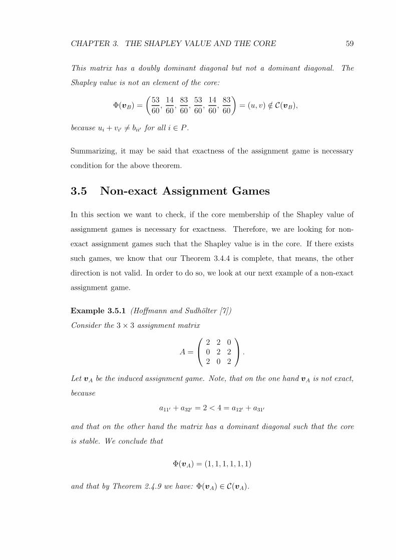
CHAPTER 3. THE SHAPLEY VALUE AND THE CORE 59
This matrix has a doubly dominant diagonal but not a dominant diagonal. The
Shapley value is not an element of the core:
Φ(vB) =
(
53
60,
14
60,
83
60,
53
60,
14
60,
83
60
)
= (u, v) /∈ C(vB),
because ui + vi′ 6= bii′ for all i ∈ P .
Summarizing, it may be said that exactness of the assignment game is necessary
condition for the above theorem.
3.5 Non-exact Assignment Games
In this section we want to check, if the core membership of the Shapley value of
assignment games is necessary for exactness. Therefore, we are looking for non-
exact assignment games such that the Shapley value is in the core. If there exists
such games, we know that our Theorem 3.4.4 is complete, that means, the other
direction is not valid. In order to do so, we look at our next example of a non-exact
assignment game.
Example 3.5.1 (Hoffmann and Sudholter [7])
Consider the 3 × 3 assignment matrix
A =
2 2 00 2 22 0 2
.
Let vA be the induced assignment game. Note, that on the one hand vA is not exact,
because
a11′ + a32′ = 2 < 4 = a12′ + a31′
and that on the other hand the matrix has a dominant diagonal such that the core
is stable. We conclude that
Φ(vA) = (1, 1, 1, 1, 1, 1)
and that by Theorem 2.4.9 we have: Φ(vA) ∈ C(vA).
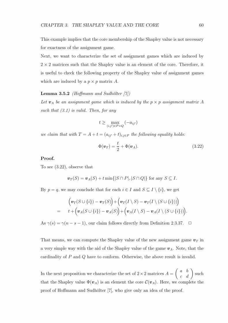
CHAPTER 3. THE SHAPLEY VALUE AND THE CORE 60
This example implies that the core membership of the Shapley value is not necessary
for exactness of the assignment game.
Next, we want to characterize the set of assignment games which are induced by
2 × 2 matrices such that the Shapley value is an element of the core. Therefore, it
is useful to check the following property of the Shapley value of assignment games
which are induced by a p × p matrix A.
Lemma 3.5.2 (Hoffmann and Sudholter [7])
Let vA be an assignment game which is induced by the p × p assignment matrix A
such that (3.1) is valid. Then, for any
t ≥ max(i,j′)∈P×Q
(−aij′)
we claim that with T = A + t = (aij′ + t)i,j∈P the following equality holds:
Φ(vT ) =t
2+ Φ(vA). (3.22)
Proof.
To see (3.22), observe that
vT (S) = vA(S) + t min{|S ∩ P |, |S ∩ Q|} for any S ⊆ I.
By p = q, we may conclude that for each i ∈ I and S ⊆ I \ {i}, we get
(
vT (S ∪ {i}) − vT (S))
+(
vT (I \ S) − vT (I \ (S ∪ {i})))
= t +(
vA(S ∪ {i}) − vA(S))
+(
vA(I \ S) − vA(I \ (S ∪ {i})))
.
As γ(s) = γ(n − s − 1), our claim follows directly from Definition 2.3.37. 2
That means, we can compute the Shapley value of the new assignment game vT in
a very simple way with the aid of the Shapley value of the game vA. Note, that the
cardinality of P and Q have to conform. Otherwise, the above result is invalid.
In the next proposition we characterize the set of 2×2 matrices A =
(
a bc d
)
such
that the Shapley value Φ(vA) is an element the core C(vA). Here, we complete the
proof of Hoffmann and Sudholter [7], who give only an idea of the proof.
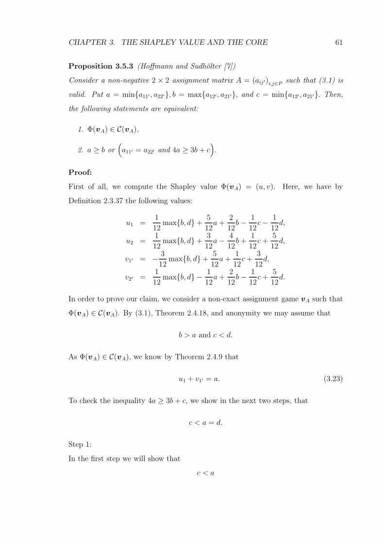
CHAPTER 3. THE SHAPLEY VALUE AND THE CORE 61
Proposition 3.5.3 (Hoffmann and Sudholter [7])
Consider a non-negative 2 × 2 assignment matrix A = (aij′)i,j∈Psuch that (3.1) is
valid. Put a = min{a11′ , a22′}, b = max{a12′ , a21′}, and c = min{a12′ , a21′}. Then,
the following statements are equivalent:
1. Φ(vA) ∈ C(vA),
2. a ≥ b or(
a11′ = a22′ and 4a ≥ 3b + c)
.
Proof:
First of all, we compute the Shapley value Φ(vA) = (u, v). Here, we have by
Definition 2.3.37 the following values:
u1 =1
12max{b, d} +
5
12a +
2
12b −
1
12c −
1
12d,
u2 =1
12max{b, d} +
3
12a −
4
12b +
1
12c +
5
12d,
v1′ = −3
12max{b, d} +
5
12a +
1
12c +
3
12d,
v2′ =1
12max{b, d} −
1
12a +
2
12b −
1
12c +
5
12d.
In order to prove our claim, we consider a non-exact assignment game vA such that
Φ(vA) ∈ C(vA). By (3.1), Theorem 2.4.18, and anonymity we may assume that
b > a and c < d.
As Φ(vA) ∈ C(vA), we know by Theorem 2.4.9 that
u1 + v1′ = a. (3.23)
To check the inequality 4a ≥ 3b + c, we show in the next two steps, that
c < a = d.
Step 1:
In the first step we will show that
c < a
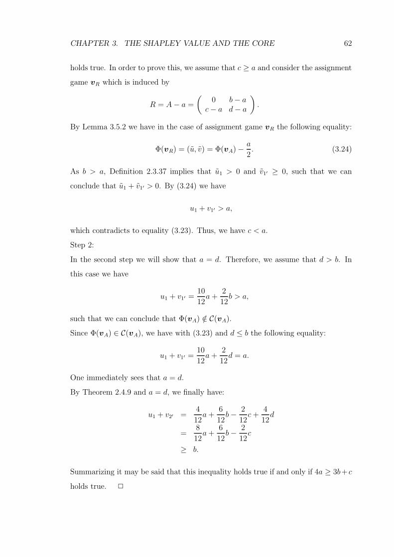
CHAPTER 3. THE SHAPLEY VALUE AND THE CORE 62
holds true. In order to prove this, we assume that c ≥ a and consider the assignment
game vR which is induced by
R = A − a =
(
0 b − ac − a d − a
)
.
By Lemma 3.5.2 we have in the case of assignment game vR the following equality:
Φ(vR) = (u, v) = Φ(vA) −a
2. (3.24)
As b > a, Definition 2.3.37 implies that u1 > 0 and v1′ ≥ 0, such that we can
conclude that u1 + v1′ > 0. By (3.24) we have
u1 + v1′ > a,
which contradicts to equality (3.23). Thus, we have c < a.
Step 2:
In the second step we will show that a = d. Therefore, we assume that d > b. In
this case we have
u1 + v1′ =10
12a +
2
12b > a,
such that we can conclude that Φ(vA) /∈ C(vA).
Since Φ(vA) ∈ C(vA), we have with (3.23) and d ≤ b the following equality:
u1 + v1′ =10
12a +
2
12d = a.
One immediately sees that a = d.
By Theorem 2.4.9 and a = d, we finally have:
u1 + v2′ =4
12a +
6
12b −
2
12c +
4
12d
=8
12a +
6
12b −
2
12c
≥ b.
Summarizing it may be said that this inequality holds true if and only if 4a ≥ 3b+ c
holds true. 2
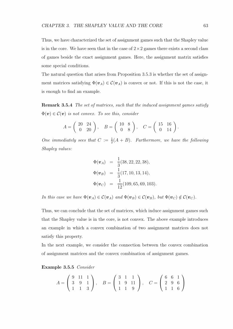
CHAPTER 3. THE SHAPLEY VALUE AND THE CORE 63
Thus, we have characterized the set of assignment games such that the Shapley value
is in the core. We have seen that in the case of 2×2 games there exists a second class
of games beside the exact assignment games. Here, the assignment matrix satisfies
some special conditions.
The natural question that arises from Proposition 3.5.3 is whether the set of assign-
ment matrices satisfying Φ(vA) ∈ C(vA) is convex or not. If this is not the case, it
is enough to find an example.
Remark 3.5.4 The set of matrices, such that the induced assignment games satisfy
Φ(v) ∈ C(v) is not convex. To see this, consider
A =
(
20 240 20
)
, B =
(
10 80 8
)
, C =
(
15 160 14
)
.
One immediately sees that C := 12(A + B). Furthermore, we have the following
Shapley values:
Φ(vA) =1
3(38, 22, 22, 38),
Φ(vB) =1
3(17, 10, 13, 14),
Φ(vC) =1
12(109, 65, 69, 103).
In this case we have Φ(vA) ∈ C(vA) and Φ(vB) ∈ C(vB), but Φ(vC) /∈ C(vC).
Thus, we can conclude that the set of matrices, which induce assignment games such
that the Shapley value is in the core, is not convex. The above example introduces
an example in which a convex combination of two assignment matrices does not
satisfy this property.
In the next example, we consider the connection between the convex combination
of assignment matrices and the convex combination of assignment games.
Example 3.5.5 Consider
A =
9 11 13 9 11 1 3
, B =
3 1 11 9 111 1 9
, C =
6 6 12 9 61 1 6
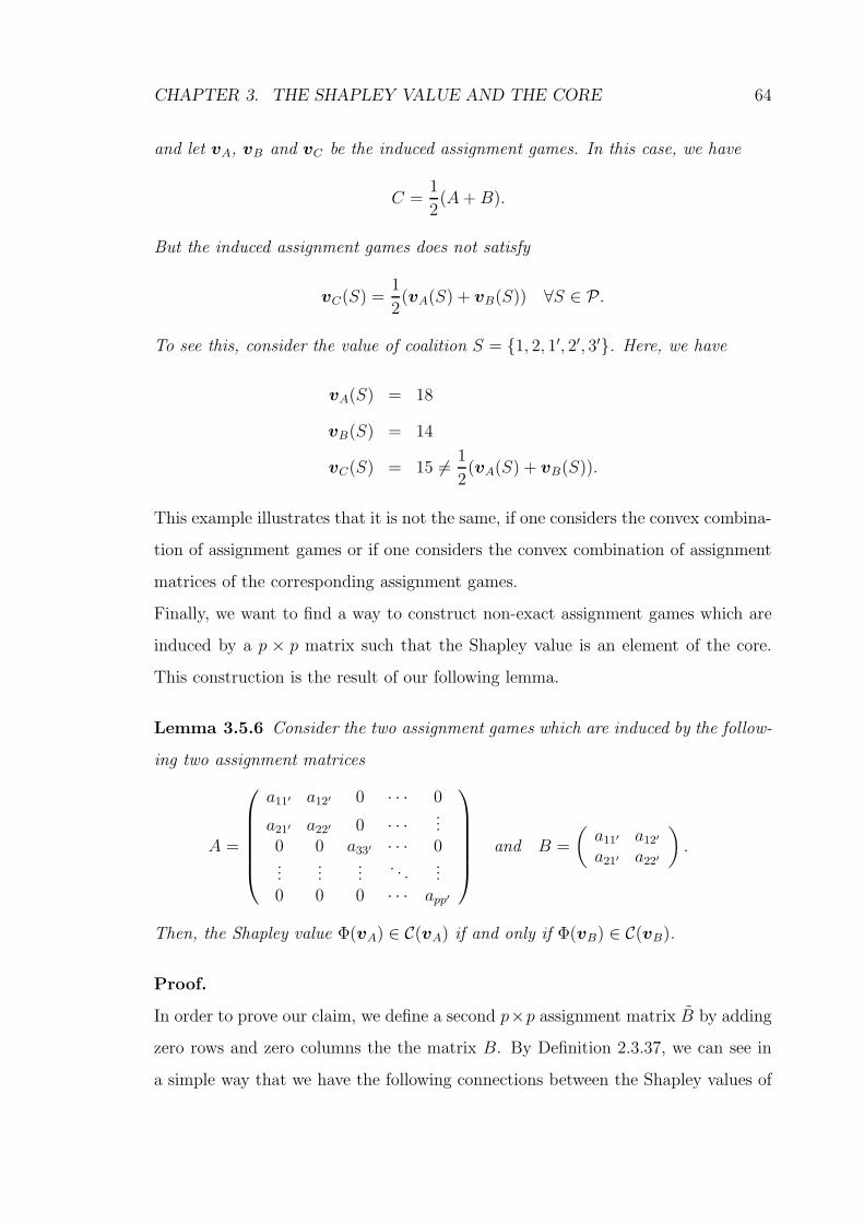
CHAPTER 3. THE SHAPLEY VALUE AND THE CORE 64
and let vA, vB and vC be the induced assignment games. In this case, we have
C =1
2(A + B).
But the induced assignment games does not satisfy
vC(S) =1
2(vA(S) + vB(S)) ∀S ∈ P.
To see this, consider the value of coalition S = {1, 2, 1′, 2′, 3′}. Here, we have
vA(S) = 18
vB(S) = 14
vC(S) = 15 6=1
2(vA(S) + vB(S)).
This example illustrates that it is not the same, if one considers the convex combina-
tion of assignment games or if one considers the convex combination of assignment
matrices of the corresponding assignment games.
Finally, we want to find a way to construct non-exact assignment games which are
induced by a p × p matrix such that the Shapley value is an element of the core.
This construction is the result of our following lemma.
Lemma 3.5.6 Consider the two assignment games which are induced by the follow-
ing two assignment matrices
A =
a11′ a12′ 0 · · · 0
a21′ a22′ 0 · · ·...
0 0 a33′ · · · 0...
......
. . ....
0 0 0 · · · app′
and B =
(
a11′ a12′
a21′ a22′
)
.
Then, the Shapley value Φ(vA) ∈ C(vA) if and only if Φ(vB) ∈ C(vB).
Proof.
In order to prove our claim, we define a second p×p assignment matrix B by adding
zero rows and zero columns the the matrix B. By Definition 2.3.37, we can see in
a simple way that we have the following connections between the Shapley values of
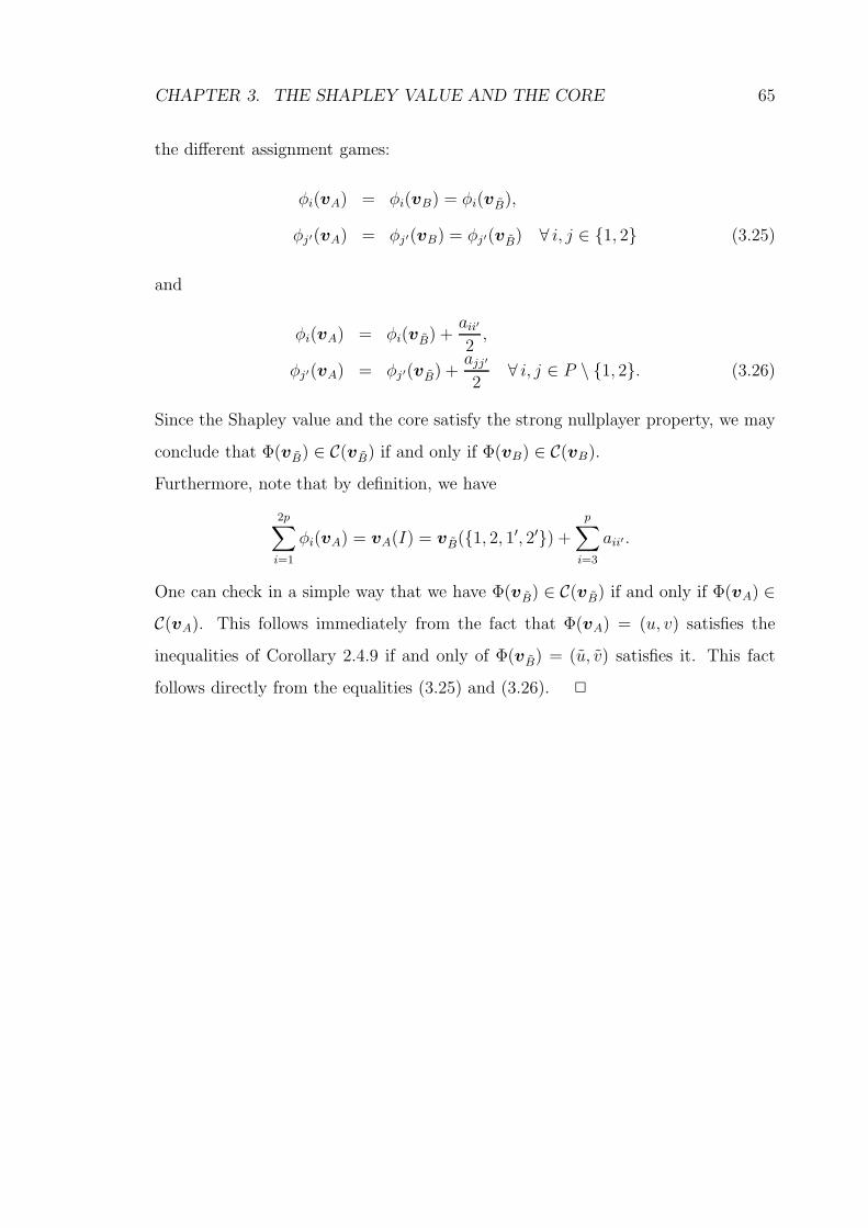
CHAPTER 3. THE SHAPLEY VALUE AND THE CORE 65
the different assignment games:
φi(vA) = φi(vB) = φi(vB),
φj′(vA) = φj′(vB) = φj′(vB) ∀ i, j ∈ {1, 2} (3.25)
and
φi(vA) = φi(vB) +aii′
2,
φj′(vA) = φj′(vB) +ajj′
2∀ i, j ∈ P \ {1, 2}. (3.26)
Since the Shapley value and the core satisfy the strong nullplayer property, we may
conclude that Φ(vB) ∈ C(vB) if and only if Φ(vB) ∈ C(vB).
Furthermore, note that by definition, we have
2p∑
i=1
φi(vA) = vA(I) = vB({1, 2, 1′, 2′}) +
p∑
i=3
aii′ .
One can check in a simple way that we have Φ(vB) ∈ C(vB) if and only if Φ(vA) ∈
C(vA). This follows immediately from the fact that Φ(vA) = (u, v) satisfies the
inequalities of Corollary 2.4.9 if and only of Φ(vB) = (u, v) satisfies it. This fact
follows directly from the equalities (3.25) and (3.26). 2
Chapter 4
The Least Core of the DualAssignment Game
4.1 Introduction
Since the modified nucleolus is an element of the least core of the dual assignment
game, we concentrate our attention on aspects of this set. In order to consider the
least core of the dual assignment game, we look at some general results of c-convex
games. C-convex games are very interesting in our context since the dual assignment
game is such a game. The most important facts in our case are the definition of these
games and some results about their least core. After having introduced c-convex
games, we continue our research with some results about the least core of a general
dual assignment game. Here, we find conditions that are satisfied by every element
of the least core. With the aid of these conditions an important result, that the
least core of dual assignment games satisfies the strong nullplayer property, can be
proved. This property allows the restriction to assignment games which are induced
by p×p matrices. A more detailed result is possible in the case of convex assignment
games. Here, we find a simple way to compute all extreme points of the least core
with the aid of the assignment matrix. Furthermore, it is possible to compute some
other solution concepts in a very simple way. In particular, we show that some of
these concepts coincide in this special case. In a next step we look for a correlation
between the least core of the dual assignment game in the case of convex games and
in the case of games with a stable core. The surprising result is that the extreme
points in the case of convex assignment games stay extreme in the more general case.
66
CHAPTER 4. THE LEAST CORE OF THE DUAL ASSIGNMENT GAME 67
Our last section is devoted to assignment games which are induced by a symmetric
p× p matrix. As in the case of convex assignment games, it is possible to find some
special properties of the least core of the dual assignment game and the modiclus.
4.2 The Least Core of C-convex Games
This section is devoted to the least core of c-convex games. It is a preparation for
the next sections where we consider the least core of dual assignment games. In
the first part of this section we look at the definition of c-convex games and some
properties. Next, we summarize some basic results of c-convex games. But now, we
start with the formal definition of c-convex games which can be found for example
in Sudholter [31].
Definition 4.2.1 Let (I,P, v) be a cooperative game and let (A, B), A, B 6= ∅,
A ∩ B = ∅ be a partition of I, this means that I = A ∪ B. The game v is comple-
mentary convex or c-convex with respect to (A, B) if and only if
v(S) + v(T ) ≤ v(
((S ∩ T ) ∩ A) ∪ ((S ∪ T ) ∩ B))
+ v(
((S ∪ T ) ∩ A) ∪ ((S ∩ T ) ∩ B))
∀S, T ∈ P.
A well-known class of c-convex games is the class of convex games. By definition
every convex game is c-convex w.r.t. (I, ∅). As in the case of convex games, note
that complementary convexness can be expressed in terms of increasing marginal
contributions of the players. To see this, we can look at the following lemma, proven
in Sudholter [31].
Lemma 4.2.2 (Sudholter [31])
Let (I,P, v) be a game and let (A, B) be a partition of I. Then, the following
statements are equivalent.
1. v is c-convex with respect to (A, B).
2.
v(S ∪ {i}) − v(S) ≤ v(T ∪ {i}) − v(T ) for i ∈ A \ T, (4.1)
v(T ∪ {j}) − v(T ) ≤ v(S ∪ {j}) − v(S) for j ∈ B \ S, (4.2)
CHAPTER 4. THE LEAST CORE OF THE DUAL ASSIGNMENT GAME 68
holds true for S, T ⊆ I with S ∩ A ⊆ T , T ∩ B ⊆ S.
3. For S ⊆ I, i, i0 ∈ A \ S, j, j0 ∈ B \ S, i 6= i0, j 6= j0 the following properties
hold:
v(S ∪ {i, j}) − v(S ∪ {j}) ≤ v(S ∪ {i}) − v(S), (4.3)
v(S ∪ {i, j}) − v(S ∪ {i}) ≤ v(S ∪ {j}) − v(S), (4.4)
v(S ∪ {i, i0}) − v(S ∪ {i}) ≥ v(S ∪ {i0}) − v(S), (4.5)
v(S ∪ {j, j0}) − v(S ∪ {j}) ≥ v(S ∪ {j0}) − v(S). (4.6)
In the case of convex games, the second statement of the above lemma implies the
same equalities as Theorem 2.2.13.
In the next step we consider a second well-known class of c-convex games, namely
the class of dual assignment games. This result dues to Sudholter [31] in 2002 and
it can be proven with the aid of Lemma 4.2.2.
Remark 4.2.3 (Sudholter [31])
The dual assignment game v?A is c-convex with respect to (P, Q).
The above remark shows the connection between c-convex games and assignment
games. In our case, it gives an incentive to pay attention on the least core of c-
convex games because the modified nucleolus of an assignment game is an element
of the least core of the dual game. Next, we are interested in a description of the
extreme points of the least core of c-convex games. For this, it is useful to have the
following definition.
Definition 4.2.4 Let (I,P, v) be a c-convex game with respect to (A, B). We define
a function γ : V → R by
γ(v) =v(A) + v(B) − v(I)
2.
Note, that in the case of dual assignment games, we have
γ(v?A) =
1
2vA(I) =
1
2v?
A(I).
CHAPTER 4. THE LEAST CORE OF THE DUAL ASSIGNMENT GAME 69
Remark 4.2.5 Sometimes we will only write γ instead of γ(v).
With the aid of Definition 4.2.4 it is possible to give a short description of a lower
bound of the maximal excess µ(x, v). In order to do so, let v be a c-convex game
w.r.t. (A, B) for some non-empty sets A and B. Furthermore, let x ∈ X(v). In
view of
2µ(x, v) ≥ v(A) − x(A) + v(B) − x(B),
= v(A) + v(B) − x(I)
= v(A) + v(B) − v(I)
= 2γ(v)
we have found a lower bound for the maximal excess of v at an arbitrary preimpu-
tation x ∈ X(v). In particular implies the definition of c-convex games that
v(I) = v(I) + v(∅) ≤ v(A) + v(B),
such that we can conclude that
γ(v) ≥ 0.
In the case of the dual assignment game v?A we have for any x ∈ X(vA) the following
inequality:
µ(x, v?A) ≥ γ(v?
A) =1
2vA(I) ≥ 0.
Before we consider the extreme points of the least core of c-convex games, we have a
look at the following lemma of Sudholter [31]. In this lemma a more simple definition
of the least core of c-convex games is given.
Lemma 4.2.6 (Sudholter[31])
Let v be a c-convex game with respect to (A, B). Then, we have
LC(v) = {x ∈ X(v) |µ(x, v) = γ(v) }.
Thus, there exist preimputations which guarantee that γ(v) is the highest possible
excess.
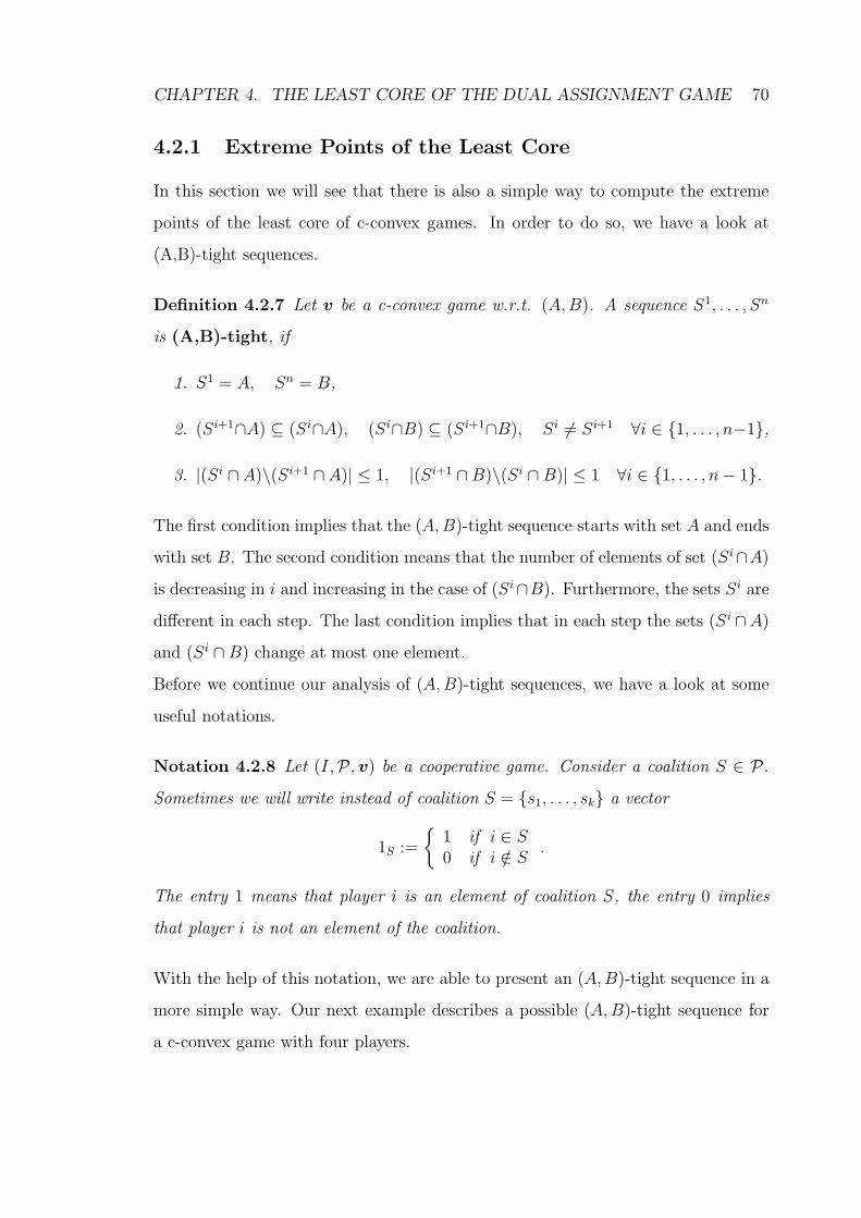
CHAPTER 4. THE LEAST CORE OF THE DUAL ASSIGNMENT GAME 70
4.2.1 Extreme Points of the Least Core
In this section we will see that there is also a simple way to compute the extreme
points of the least core of c-convex games. In order to do so, we have a look at
(A,B)-tight sequences.
Definition 4.2.7 Let v be a c-convex game w.r.t. (A, B). A sequence S1, . . . , Sn
is (A,B)-tight, if
1. S1 = A, Sn = B,
2. (Si+1∩A) ⊆ (Si∩A), (Si∩B) ⊆ (Si+1∩B), Si 6= Si+1 ∀i ∈ {1, . . . , n−1},
3. |(Si ∩ A)\(Si+1 ∩ A)| ≤ 1, |(Si+1 ∩ B)\(Si ∩ B)| ≤ 1 ∀i ∈ {1, . . . , n − 1}.
The first condition implies that the (A, B)-tight sequence starts with set A and ends
with set B. The second condition means that the number of elements of set (Si∩A)
is decreasing in i and increasing in the case of (Si∩B). Furthermore, the sets Si are
different in each step. The last condition implies that in each step the sets (Si ∩A)
and (Si ∩ B) change at most one element.
Before we continue our analysis of (A, B)-tight sequences, we have a look at some
useful notations.
Notation 4.2.8 Let (I,P, v) be a cooperative game. Consider a coalition S ∈ P.
Sometimes we will write instead of coalition S = {s1, . . . , sk} a vector
1S :=
{
1 if i ∈ S0 if i /∈ S
.
The entry 1 means that player i is an element of coalition S, the entry 0 implies
that player i is not an element of the coalition.
With the help of this notation, we are able to present an (A, B)-tight sequence in a
more simple way. Our next example describes a possible (A, B)-tight sequence for
a c-convex game with four players.
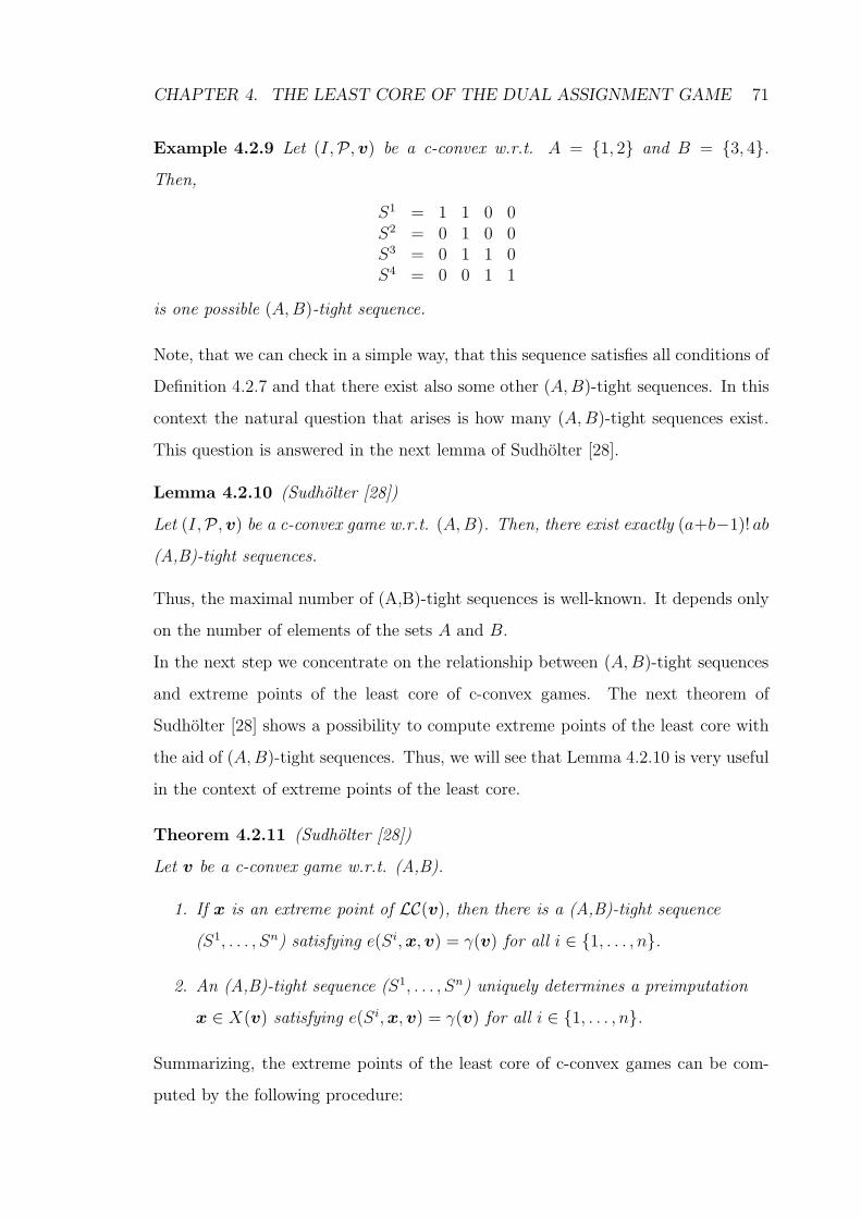
CHAPTER 4. THE LEAST CORE OF THE DUAL ASSIGNMENT GAME 71
Example 4.2.9 Let (I,P, v) be a c-convex w.r.t. A = {1, 2} and B = {3, 4}.
Then,
S1 = 1 1 0 0S2 = 0 1 0 0S3 = 0 1 1 0S4 = 0 0 1 1
is one possible (A, B)-tight sequence.
Note, that we can check in a simple way, that this sequence satisfies all conditions of
Definition 4.2.7 and that there exist also some other (A, B)-tight sequences. In this
context the natural question that arises is how many (A, B)-tight sequences exist.
This question is answered in the next lemma of Sudholter [28].
Lemma 4.2.10 (Sudholter [28])
Let (I,P, v) be a c-convex game w.r.t. (A, B). Then, there exist exactly (a+b−1)! ab
(A,B)-tight sequences.
Thus, the maximal number of (A,B)-tight sequences is well-known. It depends only
on the number of elements of the sets A and B.
In the next step we concentrate on the relationship between (A, B)-tight sequences
and extreme points of the least core of c-convex games. The next theorem of
Sudholter [28] shows a possibility to compute extreme points of the least core with
the aid of (A, B)-tight sequences. Thus, we will see that Lemma 4.2.10 is very useful
in the context of extreme points of the least core.
Theorem 4.2.11 (Sudholter [28])
Let v be a c-convex game w.r.t. (A,B).
1. If x is an extreme point of LC(v), then there is a (A,B)-tight sequence
(S1, . . . , Sn) satisfying e(Si, x, v) = γ(v) for all i ∈ {1, . . . , n}.
2. An (A,B)-tight sequence (S1, . . . , Sn) uniquely determines a preimputation
x ∈ X(v) satisfying e(Si, x, v) = γ(v) for all i ∈ {1, . . . , n}.
Summarizing, the extreme points of the least core of c-convex games can be com-
puted by the following procedure:
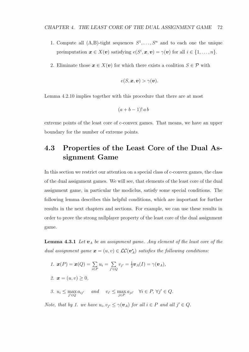
CHAPTER 4. THE LEAST CORE OF THE DUAL ASSIGNMENT GAME 72
1. Compute all (A,B)-tight sequences S1, . . . , Sn and to each one the unique
preimputation x ∈ X(v) satisfying e(Si, x, v) = γ(v) for all i ∈ {1, . . . , n}.
2. Eliminate those x ∈ X(v) for which there exists a coalition S ∈ P with
e(S, x, v) > γ(v).
Lemma 4.2.10 implies together with this procedure that there are at most
(a + b − 1)! a b
extreme points of the least core of c-convex games. That means, we have an upper
boundary for the number of extreme points.
4.3 Properties of the Least Core of the Dual As-
signment Game
In this section we restrict our attention on a special class of c-convex games, the class
of the dual assignment games. We will see, that elements of the least core of the dual
assignment game, in particular the modiclus, satisfy some special conditions. The
following lemma describes this helpful conditions, which are important for further
results in the next chapters and sections. For example, we can use these results in
order to prove the strong nullplayer property of the least core of the dual assignment
game.
Lemma 4.3.1 Let vA be an assignment game. Any element of the least core of the
dual assignment game x = (u, v) ∈ LC(v?A) satisfies the following conditions:
1. x(P ) = x(Q) =∑
i∈P
ui =∑
j′∈Q
vj′ = 12vA(I) = γ(vA),
2. x = (u, v) ≥ 0,
3. ui ≤ maxj′∈Q
aij′ and vi′ ≤ maxj∈P
aji′ ∀i ∈ P, ∀j′ ∈ Q.
Note, that by 1. we have ui, vj′ ≤ γ(vA) for all i ∈ P and all j′ ∈ Q.
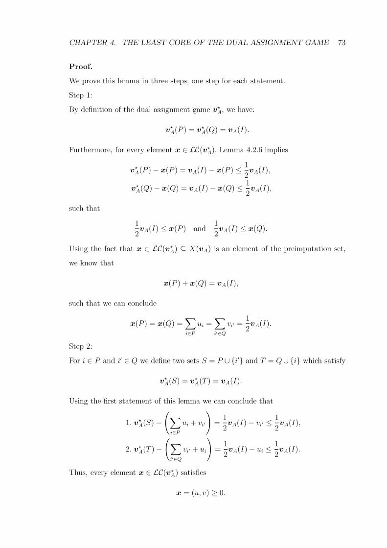
CHAPTER 4. THE LEAST CORE OF THE DUAL ASSIGNMENT GAME 73
Proof.
We prove this lemma in three steps, one step for each statement.
Step 1:
By definition of the dual assignment game v?A, we have:
v?A(P ) = v?
A(Q) = vA(I).
Furthermore, for every element x ∈ LC(v?A), Lemma 4.2.6 implies
v?A(P ) − x(P ) = vA(I) − x(P ) ≤
1
2vA(I),
v?A(Q) − x(Q) = vA(I) − x(Q) ≤
1
2vA(I),
such that
1
2vA(I) ≤ x(P ) and
1
2vA(I) ≤ x(Q).
Using the fact that x ∈ LC(v?A) ⊆ X(vA) is an element of the preimputation set,
we know that
x(P ) + x(Q) = vA(I),
such that we can conclude
x(P ) = x(Q) =∑
i∈P
ui =∑
i′∈Q
vi′ =1
2vA(I).
Step 2:
For i ∈ P and i′ ∈ Q we define two sets S = P ∪ {i′} and T = Q∪ {i} which satisfy
v?A(S) = v?
A(T ) = vA(I).
Using the first statement of this lemma we can conclude that
1. v?A(S) −
(
∑
i∈P
ui + vi′
)
=1
2vA(I) − vi′ ≤
1
2vA(I),
2. v?A(T ) −
(
∑
i′∈Q
vi′ + ui
)
=1
2vA(I) − ui ≤
1
2vA(I).
Thus, every element x ∈ LC(v?A) satisfies
x = (u, v) ≥ 0.
CHAPTER 4. THE LEAST CORE OF THE DUAL ASSIGNMENT GAME 74
Step 3:
Let i ∈ P and consider S = P\{i} such that
v?A(S) = vA(I) − max
j′∈Qaij′ .
Every element x ∈ LC(v?A) satisfies:
v?A(S) − x(S) = v?
A(I) − maxi′∈Q
aij′ −∑
j 6=i
ui ≤1
2vA(I),
i.e.1
2vA(I) − max
j′∈Qaij′ ≤
∑
j 6=i
ui =1
2vA(I) − ui.
The above inequality implies that
maxj′∈Q
aij′ ≥ ui.
Since a symmetric argument validates the case of j′ ∈ Q and T = Q \ {j′}. This
completes the proof. 2
This means that we have shown in our Lemma 4.3.1, that each element of the least
core of the dual assignment game treats the players of the two types P and Q equally.
Furthermore, we proved that all coordinates of the elements are non-negative. In
the last step we showed, that there exists an upper boundary for each coordinate of
the element of the least core of the dual assignment game.
Now, we proceed with an argumentation that it is possible to restrict our discussion
on assignment games which are introduced by a p× p assignment matrix A. There-
fore, we show that the least core of the dual assignment game satisfies the strong
nullplayer property.
Lemma 4.3.2 The least core of the dual assignment game satisfies the strong
nullplayer property.
Proof.
Let (I,P(I), vA) be an assignment game which is induced by the p × q assignment
matrix A. In order to prove the strong nullplayer property, we define a second
assignment game (I ,P(I), vA) by adding a nullplayer to the game vA. W.l.o.g. we
get the corresponding assignment matrix A from the assignment matrix A by adding
CHAPTER 4. THE LEAST CORE OF THE DUAL ASSIGNMENT GAME 75
a zero row to the matrix A.1 In this case the assignment matrix A is a (p + 1) × q
matrix. Furthermore, we have the following player sets P ⊂ P = P ∪ {p} and
Q = Q. In particular, we have by definition
vA(S) := vA(S) = vA(S ∩ I) ∀S ∈ P(I)
such that
v?A(S) := v?
A(S) = v?
A(S ∩ I) ∀ S ∈ P(I).
To show our claim, we have to prove that the following equality holds:
LC(v?A) =
{
x ∈ Rn+1 | xI ∈ LC(v?A), xp = 0
}
.
We show the above equality in two steps.
“ ⊆ “
In order to prove the first step, let x ∈ LC(v?A). By Lemma 4.3.1, every element of
the least core of the dual assignment game is non-negative and we have
x(P ) = x(Q) =1
2vA(I).
Now, remember that by definition, we have
v?A(I) = 2 γ(v?
A) = 2 γ(v?A) = v?
A(P ) = v?A(Q) = v?
A(P ) = v?A(Q).
After these general thoughts we can show that xp = 0. Since x is non-negative we
have to verify that xp > 0. Therefore, we assume that xp > 0. Then, it follows
immediately that
x(P ) > x(P ),
such that
γ(v?A) = 2 γ(v?
A) − γ(v?A)
= v?A(P ) − x(P )
< v?A(P ) − x(P )
= v?A(P ) − x(P ).
1Note, that we use a symmetric argument if we add a zero column instead of a zero row to the
matrix.
CHAPTER 4. THE LEAST CORE OF THE DUAL ASSIGNMENT GAME 76
Knowing that by Lemma 4.2.6 we have
γ(v?A) = max
S∈I
{v?A(S) − x(S)},
the contradiction follows, such that we can conclude that xp = 0.
Since xp = 0, we know that xI ∈ X(v?A). Furthermore, we have
γ(v?A) = max
S∈I
{v?A(S) − x(S)}
= maxS∈I
{v?A(S ∩ I) − x(S ∩ I)}
= maxS∈I
{v?A(S ∩ I) − xI(S)}
= maxS∈I
{v?A(S) − xI(S)}.
These properties imply that xI ∈ LC(v?A). Together with xp = 0 we have finished
our first step of the proof.
“ ⊇ “
Now, let xI ∈ LC(v?A) and let xp = 0. By definition, it follows immediately that
x ∈ X(v?A). Similar to the above part of this proof, we have
γ(v?A) = max
S∈I{v?
A(S) − xI(S)}
= maxS∈I
{v?A(S) − x(S)}
= γ(v?A),
such that we may conclude that x ∈ LC(v?A). 2
Thus, in the context of the least core of the dual assignment game, we can assume
that the assignment matrix is a p × p matrix. If this is not the case, we can add
some nullplayers until the corresponding assignment matrix is a square one. Note,
that the least core of normal games does not have to satisfy the strong nullplayer
property. In this case we have found a counter-example.
4.4 Convex Assignment Games
In this section we restrict our attention on convex assignment games and on their
least core of the dual game. Beside the result that the least core of dual assignment
CHAPTER 4. THE LEAST CORE OF THE DUAL ASSIGNMENT GAME 77
games satisfies the strong nullplayer property, we concentrate on the calculation of
elements of the least core of dual assignment game. In particular we check that it
is possible to find a simple way to calculate all extreme points of this polyhedron.
Another interesting point in this context is the connection between assignment games
with a stable core and convex assignment games, if the two assignment matrices
have the same diagonal: every extreme point of the dual least core of the convex
assignment game keeps extreme in the least core of the corresponding game.
4.4.1 Properties of the Least Core
In the case of convex assignment games it is possible to form the least core of the
dual assignment game directly from the assignment matrix. Note, that Solymosi
and Raghavan [26] proved that the assignment matrix is a diagonal matrix if and
only if the assignment game is convex. First, we will introduce some conditions
which are satisfied if we are looking at an element of the least core of the dual game.
In a next step we are looking at the extreme points. In the following theorem we
identify the least core of dual assignment game with a subset of Rn which satisfies
three conditions.
Theorem 4.4.1 Let vA be a convex assignment game which is induced by the p× p
diagonal matrix A. Then, the following statements are equivalent:
1. x = (u, v) ∈ LC(v?A) ⊆ Rp+p,
2. x = (u, v) ∈ Rp+p meets the three conditions:
(a) vA(I) = x(I), i.e. x ∈ X(vA)
(b) ui, vi′ ∈ [0, aii′] ∀i ∈ P,
(c) ui = vi′ ∀i ∈ P .
Proof.
We prove the statement of the above theorem in two steps.
“ ⊆ “:
First of all, consider an element x = (u, v) ∈ LC(v?A). In order to prove our claim
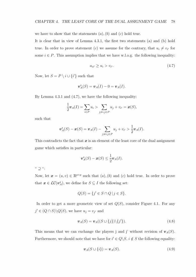
CHAPTER 4. THE LEAST CORE OF THE DUAL ASSIGNMENT GAME 78
we have to show that the statements (a), (b) and (c) hold true.
It is clear that in view of Lemma 4.3.1, the first two statements (a) and (b) hold
true. In order to prove statement (c) we assume for the contrary, that ui 6= vi′ for
some i ∈ P . This assumption implies that we have w.l.o.g. the following inequality:
aii′ ≥ ui > vi′ . (4.7)
Now, let S = P \ i ∪ {i′} such that
v?A(S) = vA(I) − 0 = vA(I).
By Lemma 4.3.1 and (4.7), we have the following inequality:
1
2vA(I) =
∑
i∈P
ui >∑
j 6=i,j∈P
uj + vi′ = x(S),
such that
v?A(S) − x(S) = vA(I) −
∑
j 6=i,j∈P
uj + vi′ >1
2vA(I).
This contradicts the fact that x is an element of the least core of the dual assignment
game which satisfies in particular:
v?A(S) − x(S) ≤
1
2vA(I).
“ ⊇ “:
Now, let x = (u, v) ∈ Rp+p such that (a), (b) and (c) hold true. In order to prove
that x ∈ LC(v?A), we define for S ⊆ I the following set:
Q(S) = {j′ ∈ S ∩ Q | j ∈ S}.
In order to get a more geometric view of set Q(S), consider Figure 4.1. For any
j′ ∈ (Q ∩ S)\Q(S), we have uj = vj′ and
vA(S) = vA((S ∪ {j})\{j′}). (4.8)
This means that we can exchange the players j and j’ without revision of vA(S).
Furthermore, we should note that we have for i′ ∈ Q\S, i /∈ S the following equality:
vA(S ∪ {i}) = vA(S). (4.9)
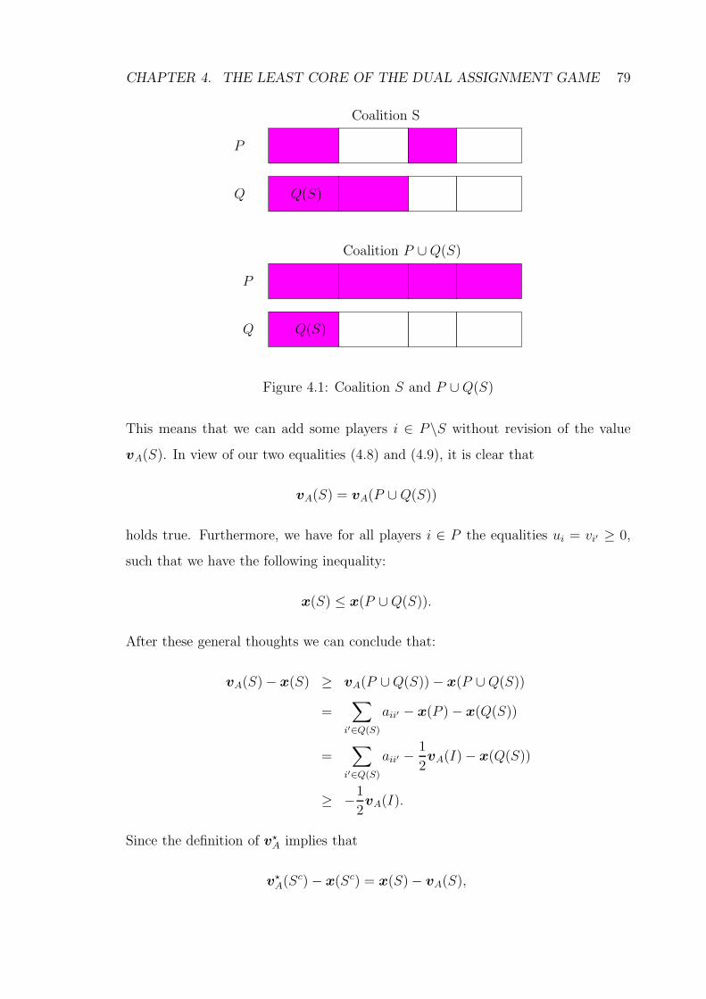
CHAPTER 4. THE LEAST CORE OF THE DUAL ASSIGNMENT GAME 79
P
P
Q
Q Q(S)
Q(S)
Coalition S
Coalition P ∪ Q(S)
Figure 4.1: Coalition S and P ∪ Q(S)
This means that we can add some players i ∈ P\S without revision of the value
vA(S). In view of our two equalities (4.8) and (4.9), it is clear that
vA(S) = vA(P ∪ Q(S))
holds true. Furthermore, we have for all players i ∈ P the equalities ui = vi′ ≥ 0,
such that we have the following inequality:
x(S) ≤ x(P ∪ Q(S)).
After these general thoughts we can conclude that:
vA(S) − x(S) ≥ vA(P ∪ Q(S)) − x(P ∪ Q(S))
=∑
i′∈Q(S)
aii′ − x(P ) − x(Q(S))
=∑
i′∈Q(S)
aii′ −1
2vA(I) − x(Q(S))
≥ −1
2vA(I).
Since the definition of v?A implies that
v?A(Sc) − x(Sc) = x(S) − vA(S),
CHAPTER 4. THE LEAST CORE OF THE DUAL ASSIGNMENT GAME 80
we can conclude that
x ∈ LC(v?A). 2
Thus, we have proved that all elements of the least core of the dual assignment
game satisfy three conditions and that all elements which satisfy these conditions
are elements of the least core of the dual assignment game. As a second step we
consider the extreme points of the least core in this special case. In the following
corollary, we show that it is possible to compute the extreme points directly from
the assignment matrix.
Corollary 4.4.2 Let A be a p×p diagonal matrix. Futhermore let vA be the induced
assignment game and let x = (u, v) ∈ LC(v?A). The element (u, v) is an extreme
point of the least core of the dual assignment game if and only if (u, v) satisfies at
least p − 1 of the following 2p conditions:
1. ui = 0 ∀i ∈ P
2. ui = aii′ ∀i ∈ P .
Our corollary shows that in the case of convex assignment games it is possible to cal-
culate the extreme points of the least core of the dual assignment game directly from
the assignment matrix. The following example demonstrates the above properties
of the extreme points of the least core of the dual assignment game.
Example 4.4.3 Consider a convex assignment game vA which is introduced by the
3 × 3 assignment matrix
A =
2 0 00 4 00 0 8
.
The extreme points of the least core of the dual game are
y1 = (0, 0, 7, 0, 0, 7), y2 = (0, 4, 3, 0, 4, 3),
y3 = (2, 0, 5, 2, 0, 5), y4 = (2, 4, 1, 2, 4, 1).
Thus, this example demonstrates how to compute the extreme points of the least
core of the dual assignment game in the case of convex games.
CHAPTER 4. THE LEAST CORE OF THE DUAL ASSIGNMENT GAME 81
4.4.2 Assignment Games with a Stable Core
This section is about assignment games with a stable core. In this case the diago-
nal of the assignment matrix supplies some extreme points of the least core of the
induced dual assignment game. We will show that the least core of the dual assign-
ment game in the case of convex assignment games is a subset of the least core in
the case of assignment games with a stable core. More formally, we have our next
lemma.
Lemma 4.4.4 Let vA be an assignment game which is induced by a p × p matrix
A such that the assignment game vA has a stable core. Furthermore, let B be the
p × p the diagonal matrix satisfying bii′ = aii′ for all i ∈ P. Then, we have
LC(v?B) ⊆ LC(v?
A).
In particular, we have
EXT LC(v?B) ⊆ EXT LC(v?
A).
Proof.
We prove our statements in two steps.
Step 1:
In the first step of the proof, we show that any element of x ∈ LC(v?B) is an element
of the least core LC(v?A). Therefore, let x ∈ LC(v?
B) ⊆ X(v?B) = X(v?
A). In order
to show that x ∈ LC(v?A) we have to demonstrate that
maxS∈P
{v?A(S) − x(S)} =
1
2vA(I).
By definition, we have for each S ∈ P the following inequality
v?A(S) ≤ v?
B(S),
such that x ∈ LC(v?B) implies
maxS∈P
{v?A(S) − x(S)} ≤
1
2vA(I). (4.10)
CHAPTER 4. THE LEAST CORE OF THE DUAL ASSIGNMENT GAME 82
Furthermore, we have for any x ∈ X(v?B) the following inequality
maxS∈P
{v?A(S) − x(S)} ≥
1
2vA(I). (4.11)
Consequently, we may conclude from (4.10) and (4.11) that x ∈ LC(v?A) such that
LC(v?B) ⊆ LC(v?
A).
Step 2:
As a second step, we want to look at the extreme points of these two polyhedrons.
One can easily see that the extreme points of LC(v?B) keeps extreme in LC(v?
A). All
extreme points y ∈ LC(v?B) satisfy the conditions of Corollary 4.4.2 and it is not
possible to find elements x1, x2 ∈ LC(v?A) which satisfy the conditions of Lemma
4.3.1 and
y = λx1 + (1 − λ)x2 λ ∈ (0, 1). 2
Our next example demonstrates that the dominant diagonal is a necessary condition
for the above lemma. In the case of assignment games without dominant diagonal
it could happen that an extreme point of the least core of the dual assignment game
does not keep extreme. Fore more details see the next example.
Example 4.4.5 Consider the following two assignment matrices A =
(
2 43 5
)
and B =
(
2 00 5
)
. Furthermore let vA and vB be the induced assignment games.
The least core LC(v?A) is defined by:
LC(v?A) = CnvH
{
(0, 3.5, 0, 3.5), (3.5, 0, 0, 3.5),
(0, 3.5, 3, 0.5), (3.5, 0, 2, 1.5),
(2.5, 1, 3, 0.5)}
In this case only one of the two extreme points x1 and x2 of LC(v?B) keeps extreme
in the least core LC(v?A). We have
x1 = (2, 1.5, 2, 1.5) /∈ EXTLC(v?A),
x2 = (0, 3.5, 0, 3.5) ∈ EXTLC(v?A).
This result is possible because ui ∈ [0, maxj′∈Q
aij′] 6⊂ [0, aii′].
CHAPTER 4. THE LEAST CORE OF THE DUAL ASSIGNMENT GAME 83
4.5 Symmetric and Exact Assignment Games
Throughout the previous section we have studied convex assignment games. By
Solymosi and Raghavan [26] these games are induced by diagonal matrices which
are particularly symmetric. In this section we restrict our attention on assignment
games which are induced by a symmetric matrix. As a second step, we consider
such games, which are also exact. But in the first step we start with the formal
definition of a symmetric matrix.
Definition 4.5.1 Let A be a m × m matrix. The matrix A is symmetric, if
aij = aji ∀i, j ∈ {1, . . . , m}.
This means, that a matrix is symmetric if and only if the matrix A and the trans-
posed matrix At are equal.
4.5.1 On some Solution Concepts
Now, we make a first attempt to compute the modiclus of assignment games. Earlier
we saw that if the assignment game has a stable core the modiclus is an element of
the core and the least core of the dual game. We show in our next theorem that this
holds true only if the assignment matrix is symmetric. In this case one can compute
the modiclus of this games in a very simple way. Furthermore, we should mention
that the modiclus is the center of gravity of the core.
Theorem 4.5.2 Let A be a symmetric p × p assignment matrix such that its main
diagonal is an optimal assignment. Furthermore let vA be the induced assignment
game. In this case we have
LC(v?A) ∩ C(vA) 6= ∅.
In particular, we have:
Ψ(vA) =1
2(a11′ , . . . , app′, a11′ , . . . , app′) ∈ LC(v?
A) ∩ C(vA).
CHAPTER 4. THE LEAST CORE OF THE DUAL ASSIGNMENT GAME 84
Note, that the second part of the proof is analogue to the proof of Raghavan and
Sudholter [12].
Proof.
We show the correctness of the statements in three steps.
Step 1:
At the beginning of the proof, we show that
m =1
2(a11′ , . . . , app′, a11′ , . . . , app′) ∈ C(vA).
Using the fact that the matrix A is symmetric, we know that (u, v) ∈ C(vA) if and
only if (v, u) ∈ C(vA). Since the main diagonal is an optimal assignment we can
conclude by Theorem 2.4.9 that
ui + vi′ = aii′ ∀i ∈ P.
Summarizing, we have
m =1
2(u, v) +
1
2(v, u) =
1
2(a11′ , . . . , app′, a11′ , . . . , app′) ∈ C(vA). (4.12)
Step 2:
In the second step of the proof we show that
m =1
2(a11′ , . . . , app′, a11′ , . . . , app′) ∈ MLC(vA). (4.13)
Therefore, we conclude that every preimputation x ∈ X(vA) implies the following
two inequalities:
1. µ(x, vA) ≥ 0
2. µ(x, v?A) ≥ 1
2vA(I).
In order to prove (4.13) we have to show that
MLC(vA) ={
x ∈ C(vA)∣
∣
∣µ(x, v?
A) =1
2vA(I)
}
. (4.14)
Equation (4.14) holds true if we can find a single element of the core that satisfies
µ(x, v?A) =
1
2vA(I).
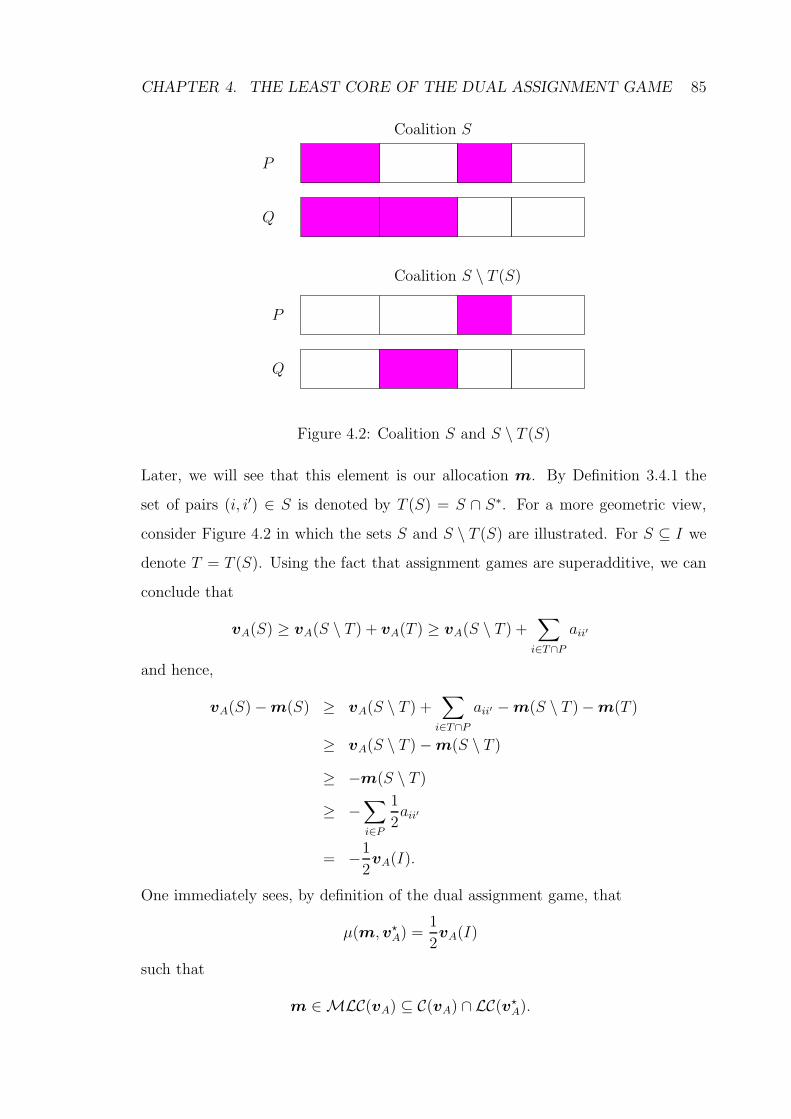
CHAPTER 4. THE LEAST CORE OF THE DUAL ASSIGNMENT GAME 85
P
P
Q
Q
Coalition S
Coalition S \ T (S)
Figure 4.2: Coalition S and S \ T (S)
Later, we will see that this element is our allocation m. By Definition 3.4.1 the
set of pairs (i, i′) ∈ S is denoted by T (S) = S ∩ S∗. For a more geometric view,
consider Figure 4.2 in which the sets S and S \ T (S) are illustrated. For S ⊆ I we
denote T = T (S). Using the fact that assignment games are superadditive, we can
conclude that
vA(S) ≥ vA(S \ T ) + vA(T ) ≥ vA(S \ T ) +∑
i∈T∩P
aii′
and hence,
vA(S) − m(S) ≥ vA(S \ T ) +∑
i∈T∩P
aii′ − m(S \ T ) − m(T )
≥ vA(S \ T ) − m(S \ T )
≥ −m(S \ T )
≥ −∑
i∈P
1
2aii′
= −1
2vA(I).
One immediately sees, by definition of the dual assignment game, that
µ(m, v?A) =
1
2vA(I)
such that
m ∈ MLC(vA) ⊆ C(vA) ∩ LC(v?A).
CHAPTER 4. THE LEAST CORE OF THE DUAL ASSIGNMENT GAME 86
Step 3:
Finally, we can conclude that in the case of a symmetric assignment matrix, we have
Ψ(vA) = (u, v) = (v, u) ∈ MLC(vA) ⊆ C(vA),
such that
ui + ui′ = aii′ ∀ i ∈ P.
All together we can conclude that
m = Ψ(vA) =1
2(a11′ , . . . , app′, a11′ , . . . , app′) ∈ C(vA) ∪ LC(v?
A). 2
With the aid of some arguments of this proof, we are able to make some thoughts
about further relations between the core and the modiclus in the case of assignment
games which are induced by a symmetric matrix. We will note in our next remark
that the modiclus is the center of gravity of the core. More precisely, we have the
following remark.
Remark 4.5.3 In the case of Theorem 4.5.2, the modiclus Ψ(vA) is the center of
gravity of the extreme points of the core and respectively to the core. This follows
from the fact that (u, v) ∈ C(vA) if and only if (v, u) ∈ C(vA).
The following lemma is concerned with different single valued solutions concepts
which are an element of the core. We will see that all these solution concepts
conform with center of gravity of the core in the case of assignment games which
are induced by symmetric assignment matrices.
Lemma 4.5.4 Let A be a symmetric p × p assignment matrix such that the main
diagonal is an optimal assignment. Furthermore, consider the assignment game vA
which is induced by A. Then, every single valued solution concept Υ(vA), which is
an element of the core C(vA), satisfies
Υ(vA) =1
2(a11′ , . . . , app′, a11′ , . . . , app′).
In particular, Υ(vA) is the center of gravity of the core.
CHAPTER 4. THE LEAST CORE OF THE DUAL ASSIGNMENT GAME 87
Proof.
Since the assignment matrix is symmetric, it follows that the solution concept is
also symmetric, i.e.
Υ(vA) = (u, v) = (v, u).
On the other hand Υ(vA) is an element of the core such that we have by Theorem
2.4.9 the following equalities:
ui + ui′ = aii′ ∀i ∈ P.
Combining these facts, we can conclude
Υ(vA) =1
2(a11′ , . . . , app′, a11′ , . . . , app′). 2
This means that, in the case of assignment games which are induced by a symmetric
assignment matrix, we know something about single valued solution concepts which
are elements of the core. These concepts conform and they can be computed in a
very simple way. Furthermore, we have found a more geometric way to compute
these concepts. To demonstrate the statement of the above lemma, consider the
following example.
Example 4.5.5 In the case of exact assignment games, which are introduced by
a symmetric matrix, particularly convex assignment games, the modiclus and the
Shapley value conform, that means, we have:
Φ(vA) = Ψ(vA) =1
2(a11′ , . . . , app′, a11′ , . . . , app′).
We mention only for reasons of completeness that the nucleolus also agree with the
Shapley value and the modiclus in this special case.
Next, we note that solution concepts of more general assignment games do not have
to conform.
Remark 4.5.6 In the case of Theorem 4.5.2 it is not necessary that the Shapley
value and the modiclus are the same, because the Shapley value is not always in the
core if the game is not exact.
CHAPTER 4. THE LEAST CORE OF THE DUAL ASSIGNMENT GAME 88
For example, we can consider the following assignment game:
Example 4.5.7 Consider the following assignment matrix A =
(
5 22 1
)
. This
matrix is symmetric but the induced assignment game vA is not exact. The Shapley
value and the modiclus are
Φ(vA) =1
3(7, 2, 7, 2),
Ψ(vA) =1
2(5, 1, 5, 1).
In particular, we have:
Φ(vA) 6= Ψ(vA) and Φ(vA) /∈ C(vA).
In the next step, we consider an exact assignment game, such that the assignment
matrix is not symmetric. Here, the Shapley value, the nucleolus, and the modified
nucleolus are elements of the core and of the least core of the dual assignment game
but the solution concepts do not conform.
Example 4.5.8 Consider the following assignment matrix A =
(
4 02 8
)
. Here,
the core and the least core of the induced assignment game vA are defined by:
C(vA) = CnvH{
(0, 0, 4, 8), (0, 8, 4, 0),
(2, 0, 2, 8), (4, 2, 0, 6), (4, 8, 0, 0)}
,
LC(v?A) = CnvH
{
(0, 6, 0, 6), (0, 6, 2, 4),
(2, 4, 4, 2), (4, 2, 4, 2)}
Furthermore, we have for the nucleolus, the modified nucleolus and the Shapley value:
ν(vA) = (2, 4, 2, 4) ,
Ψ(vA) =1
2(3, 9, 5, 7) ,
Φ(vA) =1
6(11, 25, 13, 23) .
The correlations of this example are as follows:
1. Ψ(vA) ∈ C(vA),
CHAPTER 4. THE LEAST CORE OF THE DUAL ASSIGNMENT GAME 89
2. Φ(vA) ∈ C(vA),
3. ν(vA) ∈ C(vA),
4. Φ(vA) ∈ LC(v?A),
5. ν(vA) ∈ LC(v?A),
6. Ψ(vA) 6= ν(vA) 6= Φ(vA).
Thus, we can conclude that exactness is not sufficent for different solution concepts
to conform.
4.5.2 Characteristics of the Least Core
In the above section we have considered the connection between the two elements
(u, v) and (v, u) of the core in the case of assignment games which are induced by a
symmetric matrix. Immediately, we have checked that
m =1
2(a11′ , . . . , app′, a11′ , . . . , app′) =
1
2((u, v) + (v, u))
is the center of gravity of the core. Now, we want to consider the center of gravity
of the least core of the dual assignment game. In the next lemma we show that
there exists for any x ∈ LC(v?A) a second element y ∈ LC(v?
A). With the aid of
these two elements we can compute the center of gravity of the least core of the dual
assignment game.
Lemma 4.5.9 Let vA be an exact assignment game such that the corresponding
assignment matrix A is symmetric. Then, the following statements are equivalent:
1. x = (u, v) ∈ EXT LC(v?A),
2. y = ((a11′ − u1), . . . , (app′ − up), (a11′ − v1′), . . . , (app′ − vp′)) ∈ EXT LC(v?A).
Proof.
In order to prove our claim, we show that x ∈ LC(v?A) implies that y ∈ LC(v?
A).
CHAPTER 4. THE LEAST CORE OF THE DUAL ASSIGNMENT GAME 90
The other direction follows in a similar way. Now, let x ∈ LC(v?A). In order to show
that y ∈ LC(v?A), we have to check the following equality:
vA(S) − y(S) = vA(Sc) − x(Sc) ∀S ∈ P.
For S ⊆ I define T and T as T = T (S) = S ∩ S? and T = T (Sc) = Sc ∩ (Sc)?. By
Lemma 3.4.3, we have for every coalition S the following equalities:
vA(S) − y(S) = vA(S) −∑
i∈S∩P
aii′ −∑
i′∈S∩Q
aii′ + x(S)
= vA(S \ T ) + vA(T ) −∑
i∈S∩P
aii′ −∑
i′∈S∩Q
aii′ +∑
i∈P
aii′ − x(Sc)
= vA(S \ T ) +∑
i∈T
aii′ −∑
i∈S∩P
aii′ −∑
i′∈S∩Q
aii′ +∑
i∈P
aii′ − x(Sc)
= vA(S \ T ) −∑
i∈S∩P
aii′ −∑
i′∈(S\T )∩Q
aii′ +∑
i∈P
aii′ − x(Sc)
= vA(S \ T ) − vA(T ) − x(Sc)
= vA(Sc) − x(Sc).
These equalities imply that y ∈ LC(v?A). So, we can conclude that y ∈ EXTLC(v?
A)
if and only if x ∈ EXT LC(v?A). 2
Thus, if we know one element of the least core of the dual assignment game, we can
compute a second element in a very simple way. According to Remark 4.5.3 we have
the following remark in the context of the least core of the dual assignment game.
Remark 4.5.10 In the case of Lemma 4.5.9 the following statements hold true:
1. The center of gravity of the least core of the dual assignment game is given by
m =1
2(a11′ , . . . , app′, a11′ , . . . , app′).
2. The center of gravity of the core agrees with the center of gravity of the least
core of the dual assignment game.
In the case of exact assignment games which are induced by a non-symmetric matrix,
the center of gravity of the core and the center of gravity of the least core of the
dual game are not necessarily the same. To demonstrate this certainty, we consider
the following example.
CHAPTER 4. THE LEAST CORE OF THE DUAL ASSIGNMENT GAME 91
Example 4.5.11 Consider the assignment game vA which is induced by the assign-
ment matrix
A =
(
4 24 6
)
.
Then, the center of gravity of C(vA) is (2, 4, 2, 2) and the center of gravity of LC(v?A)
is (2, 3, 2, 3).
This means that, in the case of assignment games which are induced by a non-
symmetric assignment matrix, we can not say anything about the connection of the
two centers of gravity.
Chapter 5
Assignment Games induced by2 × 2 matrices
5.1 Introduction
In this chapter we consider assignment games with a stable core which are induced
by 2× 2 matrices. We mainly focus on the core and the least core of the dual game.
Before we compute the extreme points of the two polyhedrons we start with a mix-
ture of an analytic and geometric consideration of both sets. The geometric results
are very helpful for computing the extreme points of the non-empty intersection of
the two sets. At the end of this chapter we take a short look at two examples in
which the intersection is only a single point. One can easily check that this point is
the modified nucleolus of the assignment game. During this chapter we restrict our
attention to assignment games which are induced by 2×2 matrices with a dominant
diagonal. Furthermore, we make the non-restrictive assumption that a11′ ≤ a22′
holds true.
5.2 The Least Core of Dual Assignment Games
This section is about the least core of the dual assignment game in the case that
the assignment matrix is a 2 × 2 matrix with a dominant diagonal. But before we
start with our description of the least core of the dual assignment game, we consider
a special kind of polyhedrons. First of all, we give the formal definition of these
subsets of Rn.
92
CHAPTER 5. ASSIGNMENT GAMES INDUCED BY 2 × 2 MATRICES 93
Definition 5.2.1 For n ∈ N the unit simplex of Rn is defined by:
Xn ={
x ∈ Rn+ |
n∑
i=1
xi = 1}
.
Let α ∈ R+. Another simplex is defined by:
α · Xn ={
x ∈ Rn+ |
n∑
i=1
xi = α}
.
Summarizing we can say that the unit simplex of Rn denotes the set of non-negative
vectors x ∈ Rn, which have the property that the sum of the coordinates is equal
to one.
Now, let vA be the assignment game which is induced by the assignment matrix
A. Lemma 4.2.6 and Lemma 4.3.1 imply that the least core of the dual assignment
game is a subset of the simplex vA(I)·Xn ⊂ Rn. In particular, we have the following
two equalities for the case of the least core of the dual assignment game:
u1 + u2 = γ and v1′ + v2′ = γ.
Thus, w.l.o.g. it is sufficient to know the two coordinates u1 ∈ [0, γ] and v1′ ∈ [0, γ].
In order to form a geometric idea of the least core of the dual assignment game, we
look at the subset
F = {(u1, v1′) | u1, v1′ ∈ [0, γ]} ⊆ R2.
Next, we define a mapping
M : F → R4
(u1, v1′) 7→ (u1, γ − u1, v1′ , γ − v1′).
The motivation of the above mapping and the set F becomes completely evident
when we note that the least core of the dual assignment game is by definition a
subset of
M(F ) = {M(u1, v1′) | (u1, v1′) ∈ F}.
This means that we have more formally:
LC(v?A) ⊆ M(F ) = CnvH
{
(γ, 0, 0, γ), (0, γ, 0, γ), (0, γ, γ, 0), (γ, 0, γ, 0)}
⊂ vA(I) · X4. (5.1)
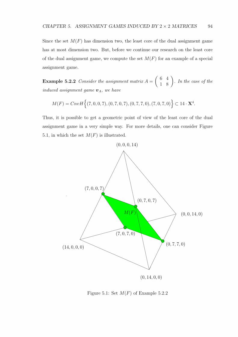
CHAPTER 5. ASSIGNMENT GAMES INDUCED BY 2 × 2 MATRICES 94
Since the set M(F ) has dimension two, the least core of the dual assignment game
has at most dimension two. But, before we continue our research on the least core
of the dual assignment game, we compute the set M(F ) for an example of a special
assignment game.
Example 5.2.2 Consider the assignment matrix A =
(
6 41 8
)
. In the case of the
induced assignment game vA, we have
M(F ) = CnvH{
(7, 0, 0, 7), (0, 7, 0, 7), (0, 7, 7, 0), (7, 0, 7, 0)}
⊂ 14 · X4.
Thus, it is possible to get a geometric point of view of the least core of the dual
assignment game in a very simple way. For more details, one can consider Figure
5.1, in which the set M(F ) is illustrated.
M(F )
(14, 0, 0, 0)
(0, 14, 0, 0)
(0, 0, 14, 0)
(0, 0, 0, 14)
(7, 0, 7, 0)
(0, 7, 7, 0)
(0, 7, 0, 7)
(7, 0, 0, 7)
Figure 5.1: Set M(F ) of Example 5.2.2
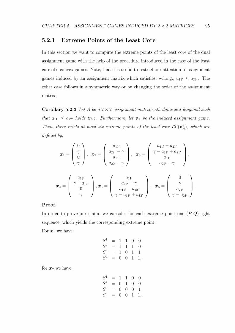
CHAPTER 5. ASSIGNMENT GAMES INDUCED BY 2 × 2 MATRICES 95
5.2.1 Extreme Points of the Least Core
In this section we want to compute the extreme points of the least core of the dual
assignment game with the help of the procedure introduced in the case of the least
core of c-convex games. Note, that it is useful to restrict our attention to assignment
games induced by an assignment matrix which satisfies, w.l.o.g., a11′ ≤ a22′ . The
other case follows in a symmetric way or by changing the order of the assignment
matrix.
Corollary 5.2.3 Let A be a 2 × 2 assignment matrix with dominant diagonal such
that a11′ ≤ a22′ holds true. Furthermore, let vA be the induced assignment game.
Then, there exists at most six extreme points of the least core LC(v?A), which are
defined by:
x1 =
0γ0γ
, x2 =
a11′
a22′ − γa11′
a22′ − γ
, x3 =
a11′ − a21′
γ − a11′ + a21′
a11′
a22′ − γ
,
x4 =
a12′
γ − a12′
0γ
, x5 =
a11′
a22′ − γa11′ − a12′
γ − a11′ + a12′
, x6 =
0γ
a21′
γ − a21′
.
Proof.
In order to prove our claim, we consider for each extreme point one (P, Q)-tight
sequence, which yields the corresponding extreme point.
For x1 we have:
S1 = 1 1 0 0S2 = 1 1 1 0S3 = 1 0 1 1S4 = 0 0 1 1,
for x2 we have:
S1 = 1 1 0 0S2 = 0 1 0 0S3 = 0 0 0 1S4 = 0 0 1 1,
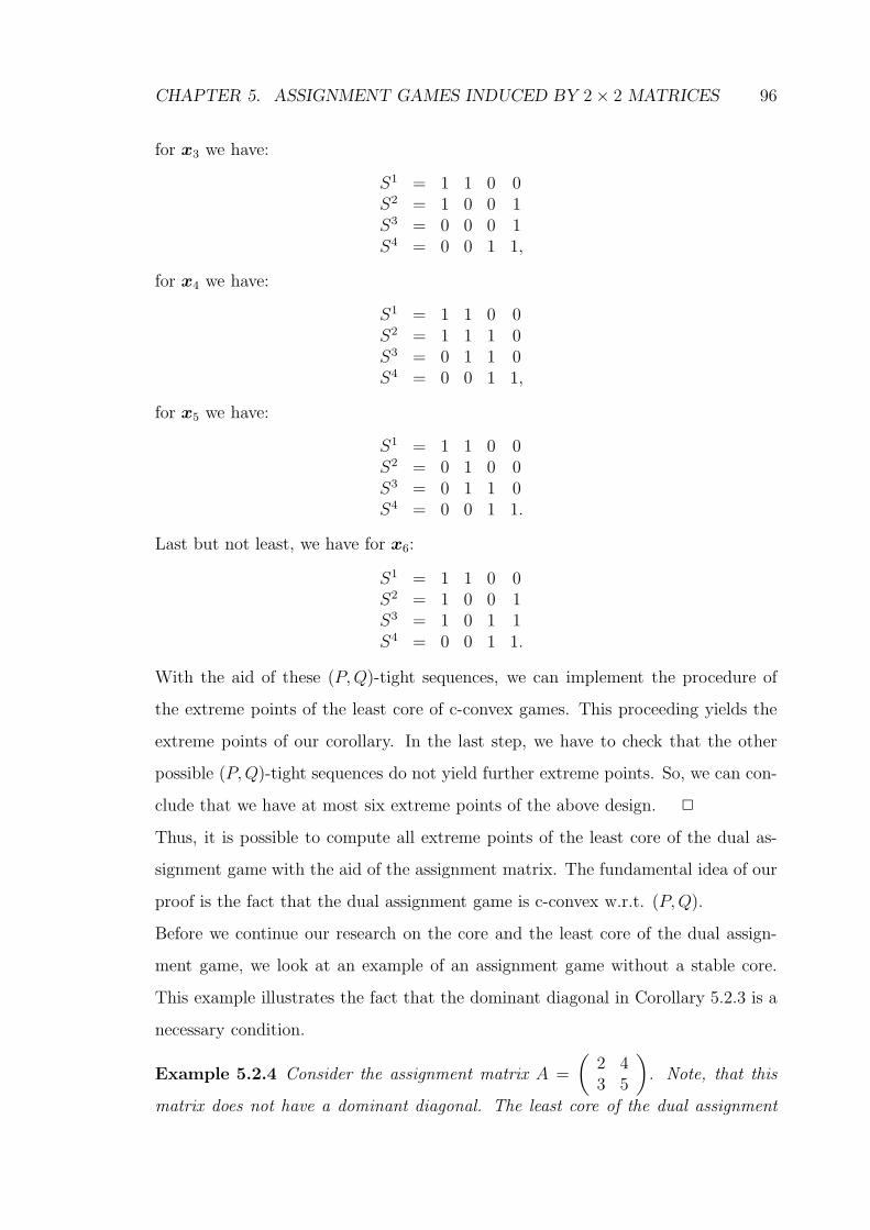
CHAPTER 5. ASSIGNMENT GAMES INDUCED BY 2 × 2 MATRICES 96
for x3 we have:
S1 = 1 1 0 0S2 = 1 0 0 1S3 = 0 0 0 1S4 = 0 0 1 1,
for x4 we have:
S1 = 1 1 0 0S2 = 1 1 1 0S3 = 0 1 1 0S4 = 0 0 1 1,
for x5 we have:
S1 = 1 1 0 0S2 = 0 1 0 0S3 = 0 1 1 0S4 = 0 0 1 1.
Last but not least, we have for x6:
S1 = 1 1 0 0S2 = 1 0 0 1S3 = 1 0 1 1S4 = 0 0 1 1.
With the aid of these (P, Q)-tight sequences, we can implement the procedure of
the extreme points of the least core of c-convex games. This proceeding yields the
extreme points of our corollary. In the last step, we have to check that the other
possible (P, Q)-tight sequences do not yield further extreme points. So, we can con-
clude that we have at most six extreme points of the above design. 2
Thus, it is possible to compute all extreme points of the least core of the dual as-
signment game with the aid of the assignment matrix. The fundamental idea of our
proof is the fact that the dual assignment game is c-convex w.r.t. (P, Q).
Before we continue our research on the core and the least core of the dual assign-
ment game, we look at an example of an assignment game without a stable core.
This example illustrates the fact that the dominant diagonal in Corollary 5.2.3 is a
necessary condition.
Example 5.2.4 Consider the assignment matrix A =
(
2 43 5
)
. Note, that this
matrix does not have a dominant diagonal. The least core of the dual assignment
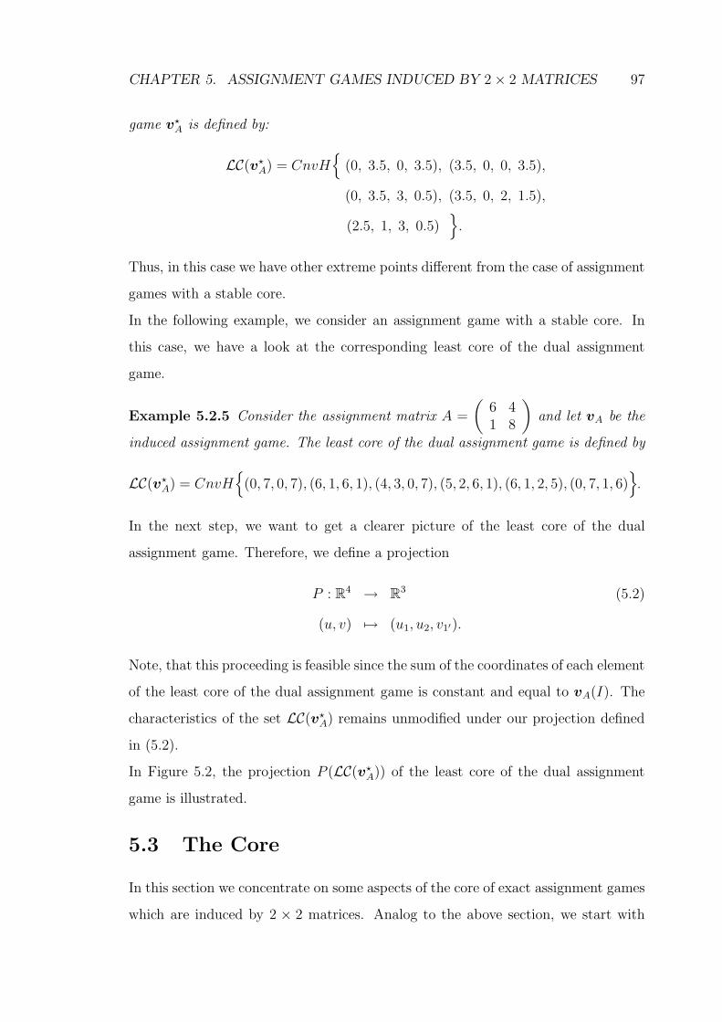
CHAPTER 5. ASSIGNMENT GAMES INDUCED BY 2 × 2 MATRICES 97
game v?A is defined by:
LC(v?A) = CnvH
{
(0, 3.5, 0, 3.5), (3.5, 0, 0, 3.5),
(0, 3.5, 3, 0.5), (3.5, 0, 2, 1.5),
(2.5, 1, 3, 0.5)}
.
Thus, in this case we have other extreme points different from the case of assignment
games with a stable core.
In the following example, we consider an assignment game with a stable core. In
this case, we have a look at the corresponding least core of the dual assignment
game.
Example 5.2.5 Consider the assignment matrix A =
(
6 41 8
)
and let vA be the
induced assignment game. The least core of the dual assignment game is defined by
LC(v?A) = CnvH
{
(0, 7, 0, 7), (6, 1, 6, 1), (4, 3, 0, 7), (5, 2, 6, 1), (6, 1, 2, 5), (0, 7, 1, 6)}
.
In the next step, we want to get a clearer picture of the least core of the dual
assignment game. Therefore, we define a projection
P : R4 → R3 (5.2)
(u, v) 7→ (u1, u2, v1′).
Note, that this proceeding is feasible since the sum of the coordinates of each element
of the least core of the dual assignment game is constant and equal to vA(I). The
characteristics of the set LC(v?A) remains unmodified under our projection defined
in (5.2).
In Figure 5.2, the projection P (LC(v?A)) of the least core of the dual assignment
game is illustrated.
5.3 The Core
In this section we concentrate on some aspects of the core of exact assignment games
which are induced by 2 × 2 matrices. Analog to the above section, we start with
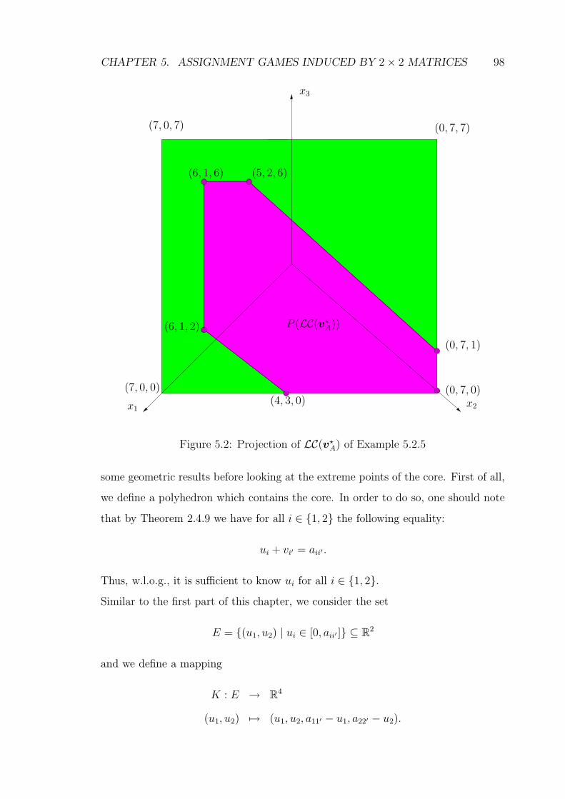
CHAPTER 5. ASSIGNMENT GAMES INDUCED BY 2 × 2 MATRICES 98
x1
x3
x2(4, 3, 0)
(7, 0, 0) (0, 7, 0)
(6, 1, 2)
(0, 7, 1)
(6, 1, 6) (5, 2, 6)
(7, 0, 7) (0, 7, 7)
P (LC(v?A))
Figure 5.2: Projection of LC(v?A) of Example 5.2.5
some geometric results before looking at the extreme points of the core. First of all,
we define a polyhedron which contains the core. In order to do so, one should note
that by Theorem 2.4.9 we have for all i ∈ {1, 2} the following equality:
ui + vi′ = aii′ .
Thus, w.l.o.g., it is sufficient to know ui for all i ∈ {1, 2}.
Similar to the first part of this chapter, we consider the set
E = {(u1, u2) | ui ∈ [0, aii′ ]} ⊆ R2
and we define a mapping
K : E → R4
(u1, u2) 7→ (u1, u2, a11′ − u1, a22′ − u2).
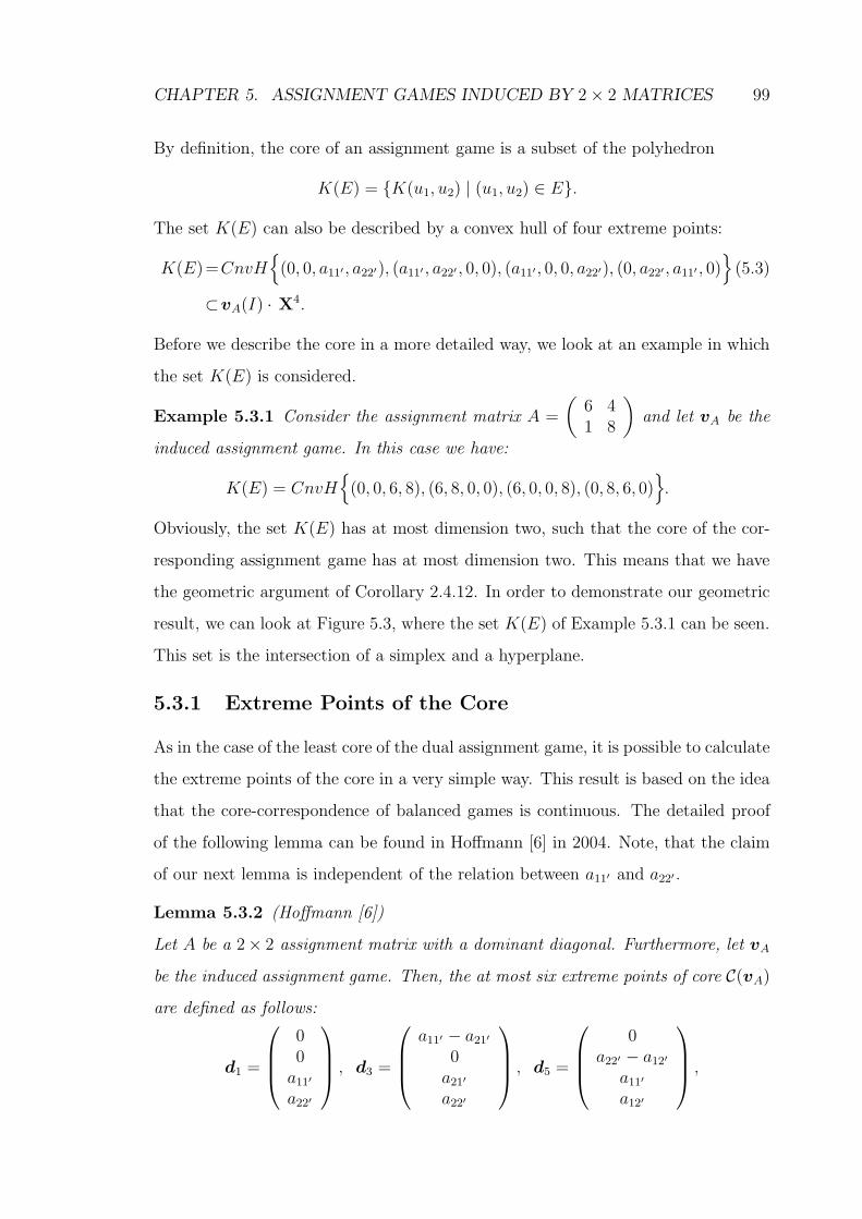
CHAPTER 5. ASSIGNMENT GAMES INDUCED BY 2 × 2 MATRICES 99
By definition, the core of an assignment game is a subset of the polyhedron
K(E) = {K(u1, u2) | (u1, u2) ∈ E}.
The set K(E) can also be described by a convex hull of four extreme points:
K(E)=CnvH{
(0, 0, a11′, a22′), (a11′ , a22′ , 0, 0), (a11′, 0, 0, a22′), (0, a22′, a11′ , 0)}
(5.3)
⊂vA(I) · X4.
Before we describe the core in a more detailed way, we look at an example in which
the set K(E) is considered.
Example 5.3.1 Consider the assignment matrix A =
(
6 41 8
)
and let vA be the
induced assignment game. In this case we have:
K(E) = CnvH{
(0, 0, 6, 8), (6, 8, 0, 0), (6, 0, 0, 8), (0, 8, 6, 0)}
.
Obviously, the set K(E) has at most dimension two, such that the core of the cor-
responding assignment game has at most dimension two. This means that we have
the geometric argument of Corollary 2.4.12. In order to demonstrate our geometric
result, we can look at Figure 5.3, where the set K(E) of Example 5.3.1 can be seen.
This set is the intersection of a simplex and a hyperplane.
5.3.1 Extreme Points of the Core
As in the case of the least core of the dual assignment game, it is possible to calculate
the extreme points of the core in a very simple way. This result is based on the idea
that the core-correspondence of balanced games is continuous. The detailed proof
of the following lemma can be found in Hoffmann [6] in 2004. Note, that the claim
of our next lemma is independent of the relation between a11′ and a22′ .
Lemma 5.3.2 (Hoffmann [6])
Let A be a 2× 2 assignment matrix with a dominant diagonal. Furthermore, let vA
be the induced assignment game. Then, the at most six extreme points of core C(vA)
are defined as follows:
d1 =
00
a11′
a22′
, d3 =
a11′ − a21′
0a21′
a22′
, d5 =
0a22′ − a12′
a11′
a12′
,
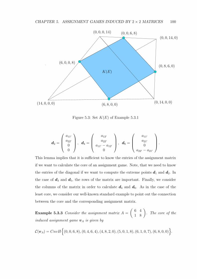
CHAPTER 5. ASSIGNMENT GAMES INDUCED BY 2 × 2 MATRICES 100
(14, 0, 0, 0) (6, 8, 0, 0)
(0, 8, 6, 0)(6, 0, 0, 8)
(0, 14, 0, 0)
(0, 0, 14, 0)(0, 0, 6, 8)(0, 0, 0, 14)
K(E)
Figure 5.3: Set K(E) of Example 5.3.1
d2 =
a11′
a22′
00
, d4 =
a12′
a22′
a11′ − a12′
0
, d6 =
a11′
a21′
0a22′ − a21′
.
This lemma implies that it is sufficient to know the entries of the assignment matrix
if we want to calculate the core of an assignment game. Note, that we need to know
the entries of the diagonal if we want to compute the extreme points d1 and d2. In
the case of d3 and d5, the rows of the matrix are important. Finally, we consider
the columns of the matrix in order to calculate d4 and d6. As in the case of the
least core, we consider our well-known standard example to point out the connection
between the core and the corresponding assignment matrix.
Example 5.3.3 Consider the assignment matrix A =
(
6 41 8
)
. The core of the
induced assignment game vA is given by
C(vA) = CnvH{
(0, 0, 6, 8), (0, 4, 6, 4), (4, 8, 2, 0), (5, 0, 1, 8), (6, 1, 0, 7), (6, 8, 0, 0)}
.
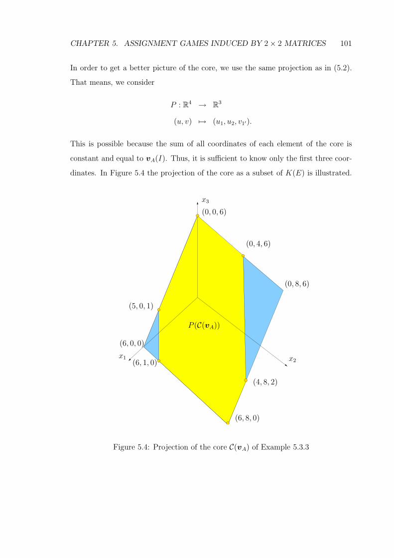
CHAPTER 5. ASSIGNMENT GAMES INDUCED BY 2 × 2 MATRICES 101
In order to get a better picture of the core, we use the same projection as in (5.2).
That means, we consider
P : R4 → R3
(u, v) 7→ (u1, u2, v1′).
This is possible because the sum of all coordinates of each element of the core is
constant and equal to vA(I). Thus, it is sufficient to know only the first three coor-
dinates. In Figure 5.4 the projection of the core as a subset of K(E) is illustrated.
x1
x3
x2
P (C(vA))
(6, 8, 0)
(6, 1, 0)
(6, 0, 0)
(5, 0, 1)
(4, 8, 2)
(0, 8, 6)
(0, 4, 6)
(0, 0, 6)
Figure 5.4: Projection of the core C(vA) of Example 5.3.3
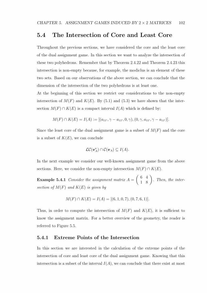
CHAPTER 5. ASSIGNMENT GAMES INDUCED BY 2 × 2 MATRICES 102
5.4 The Intersection of Core and Least Core
Throughout the previous sections, we have considered the core and the least core
of the dual assignment game. In this section we want to analyze the intersection of
these two polyhedrons. Remember that by Theorem 2.4.22 and Theorem 2.4.23 this
intersection is non-empty because, for example, the modiclus is an element of these
two sets. Based on our observations of the above section, we can conclude that the
dimension of the intersection of the two polyhedrons is at least one.
At the beginning of this section we restrict our considerations to the non-empty
intersection of M(F ) and K(E). By (5.1) and (5.3) we have shown that the inter-
section M(F ) ∩ K(E) is a compact interval I(A) which is defined by:
M(F ) ∩ K(E) = I(A) := [(a11′ , γ − a11′ , 0, γ), (0, γ, a11′, γ − a11′)].
Since the least core of the dual assignment game is a subset of M(F ) and the core
is a subset of K(E), we can conclude
LC(v?A) ∩ C(vA) ⊆ I(A).
In the next example we consider our well-known assignment game from the above
sections. Here, we consider the non-empty intersection M(F ) ∩ K(E).
Example 5.4.1 Consider the assignment matrix A =
(
6 41 8
)
. Then, the inter-
section of M(F ) and K(E) is given by
M(F ) ∩ K(E) = I(A) = [(6, 1, 0, 7), (0, 7, 6, 1)].
Thus, in order to compute the intersection of M(F ) and K(E), it is sufficient to
know the assignment matrix. For a better overview of the geometry, the reader is
referred to Figure 5.5.
5.4.1 Extreme Points of the Intersection
In this section we are interested in the calculation of the extreme points of the
intersection of core and least core of the dual assignment game. Knowing that this
intersection is a subset of the interval I(A), we can conclude that there exist at most
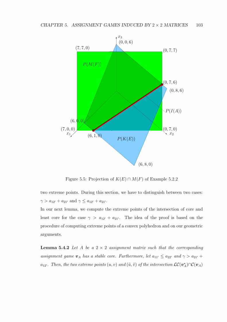
CHAPTER 5. ASSIGNMENT GAMES INDUCED BY 2 × 2 MATRICES 103
x1
x3
x2
(7, 0, 0)
(6, 1, 0)
(6, 8, 0)
(0, 8, 6)
(0, 7, 6)
(0, 7, 7)
(0, 0, 6)
(7, 7, 0)
(0, 7, 0)
P (M(F ))
P (K(E))
P (I(A))
(6, 0, 0)
Figure 5.5: Projection of K(E) ∩ M(F ) of Example 5.2.2
two extreme points. During this section, we have to distinguish between two cases:
γ > a12′ + a21′ and γ ≤ a12′ + a21′ .
In our next lemma, we compute the extreme points of the intersection of core and
least core for the case γ > a12′ + a21′ . The idea of the proof is based on the
procedure of computing extreme points of a convex polyhedron and on our geometric
arguments.
Lemma 5.4.2 Let A be a 2 × 2 assignment matrix such that the corresponding
assignment game vA has a stable core. Furthermore, let a11′ ≤ a22′ and γ > a21′ +
a12′ . Then, the two extreme points (u, v) and (u, v) of the intersection LC(v?A)∩C(vA)
CHAPTER 5. ASSIGNMENT GAMES INDUCED BY 2 × 2 MATRICES 104
are defined as follows:
u1 =a12′
2+
a11′
2,
u2 = γ −a12′
2−
a11′
2,
v1′ =a11′
2−
a12′
2,
v2′ = γ +a12′
2−
a11′
2,
and
u1 =a11′
2−
a21′
2,
u2 = γ −a11′
2+
a21′
2,
v1′ =a11′
2+
a21′
2,
v2′ = γ −a21′
2−
a11′
2.
Proof.
We show that (u, v) and (u, v) are elements of the core C(vA) and of the least core
of the dual assignment game LC(v?A). Therefore, we have to check the inequalities
which describe the two polyhedrons. Last but not least we have to find for each
extreme point (u, v) and (u, v) four inequalities such that
1. the corresponding inequalities are equalities,
2. the extreme point is the unique solution of a system of equalities.
In the steps 1a and 2a of the proof, we show that the point (u, v) is an element of
C(vA) and LC(v?A). In step 3a, we point out a system of four equalities with unique
solution (u, v). Then, we repeat the procedure in step 1b, 2b and 3b for the second
point (u, v). Remember that it is not possible to have more than two extreme points,
because the dimension of the intersection is at most one.
Step 1a:
We show in our first step that
x = (u, v) ∈ C(vA)
holds.
CHAPTER 5. ASSIGNMENT GAMES INDUCED BY 2 × 2 MATRICES 105
By Theorem 2.4.9 we have to check the following three inequalities:
1. (u, v) ≥ 0,
2.∑
i∈P ui +∑
j′∈Q vj′ =∑
i∈P aii′ ,
3. ui + vj′ ≥ aij′ ∀ i, j ∈ P .
Since the assignment matrix A has a dominant diagonal, the inequality
(u, v) ≥ 0
follows by definition. Furthermore, we can conclude
∑
i∈P
ui +∑
j′∈Q
vj′ = 2γ =∑
i∈P
aii′.
Since γ > a12′ + a21′ , we have
u1 + v1′ = a11′ ,
u1 + v2′ = γ + a12′ ≥ a12′ ,
u2 + v1′ = γ − a12′ > a21′ ,
u2 + v2′ = a11′ + a22′ − a11′ = a22′ ,
hence we can conclude (u, v) ∈ C(vA).
Step 2a:
In order to show that (u, v) is an element of the least core of the dual assignment
game, we have to check that for x = (u, v) the following equality
maxS∈P
e(S, x, v?A) = γ
holds true.
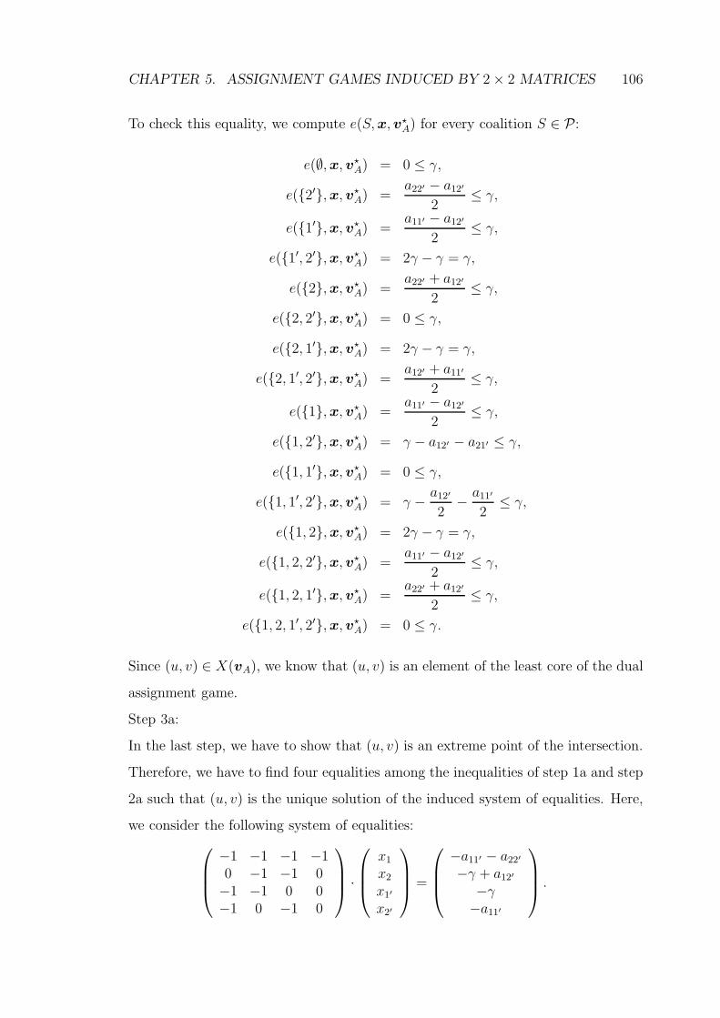
CHAPTER 5. ASSIGNMENT GAMES INDUCED BY 2 × 2 MATRICES 106
To check this equality, we compute e(S, x, v?A) for every coalition S ∈ P:
e(∅, x, v?A) = 0 ≤ γ,
e({2′}, x, v?A) =
a22′ − a12′
2≤ γ,
e({1′}, x, v?A) =
a11′ − a12′
2≤ γ,
e({1′, 2′}, x, v?A) = 2γ − γ = γ,
e({2}, x, v?A) =
a22′ + a12′
2≤ γ,
e({2, 2′}, x, v?A) = 0 ≤ γ,
e({2, 1′}, x, v?A) = 2γ − γ = γ,
e({2, 1′, 2′}, x, v?A) =
a12′ + a11′
2≤ γ,
e({1}, x, v?A) =
a11′ − a12′
2≤ γ,
e({1, 2′}, x, v?A) = γ − a12′ − a21′ ≤ γ,
e({1, 1′}, x, v?A) = 0 ≤ γ,
e({1, 1′, 2′}, x, v?A) = γ −
a12′
2−
a11′
2≤ γ,
e({1, 2}, x, v?A) = 2γ − γ = γ,
e({1, 2, 2′}, x, v?A) =
a11′ − a12′
2≤ γ,
e({1, 2, 1′}, x, v?A) =
a22′ + a12′
2≤ γ,
e({1, 2, 1′, 2′}, x, v?A) = 0 ≤ γ.
Since (u, v) ∈ X(vA), we know that (u, v) is an element of the least core of the dual
assignment game.
Step 3a:
In the last step, we have to show that (u, v) is an extreme point of the intersection.
Therefore, we have to find four equalities among the inequalities of step 1a and step
2a such that (u, v) is the unique solution of the induced system of equalities. Here,
we consider the following system of equalities:
−1 −1 −1 −10 −1 −1 0−1 −1 0 0−1 0 −1 0
·
x1
x2
x1′
x2′
=
−a11′ − a22′
−γ + a12′
−γ−a11′
.
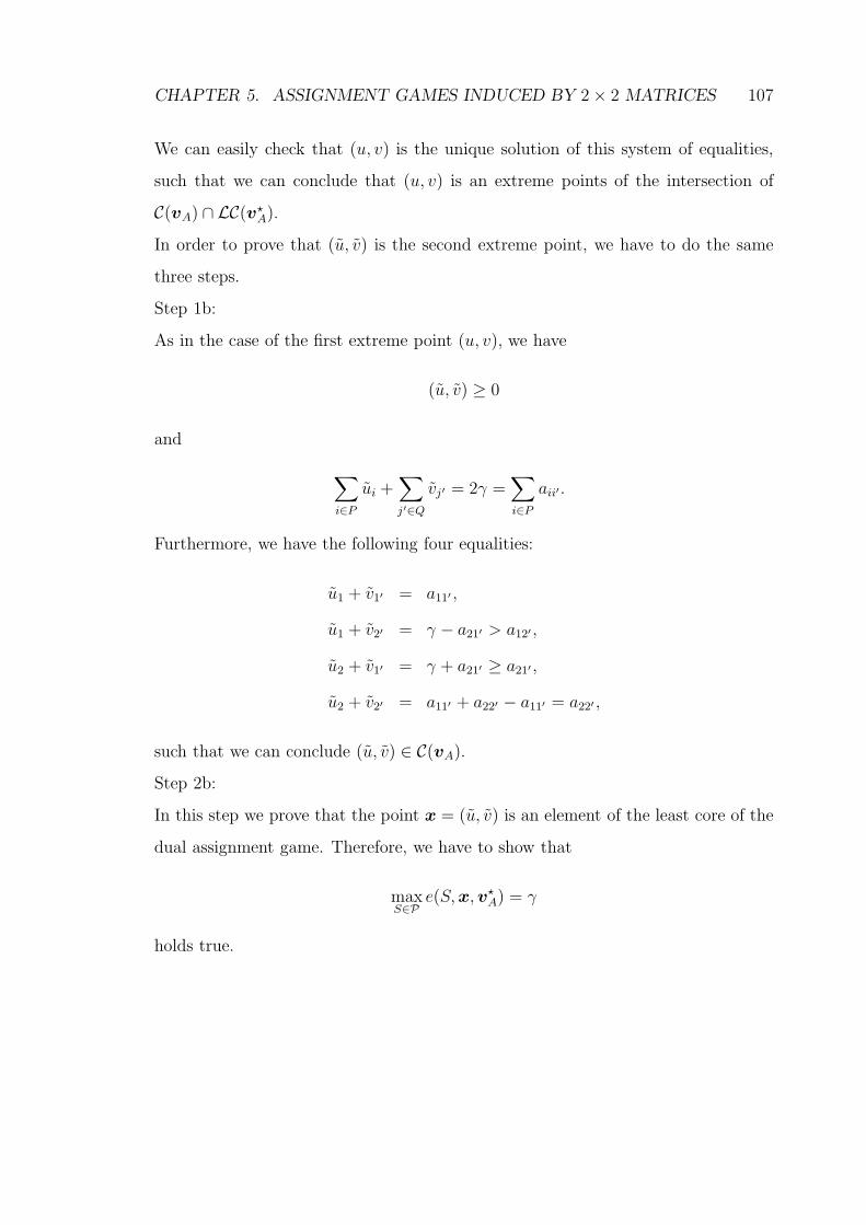
CHAPTER 5. ASSIGNMENT GAMES INDUCED BY 2 × 2 MATRICES 107
We can easily check that (u, v) is the unique solution of this system of equalities,
such that we can conclude that (u, v) is an extreme points of the intersection of
C(vA) ∩ LC(v?A).
In order to prove that (u, v) is the second extreme point, we have to do the same
three steps.
Step 1b:
As in the case of the first extreme point (u, v), we have
(u, v) ≥ 0
and
∑
i∈P
ui +∑
j′∈Q
vj′ = 2γ =∑
i∈P
aii′.
Furthermore, we have the following four equalities:
u1 + v1′ = a11′ ,
u1 + v2′ = γ − a21′ > a12′ ,
u2 + v1′ = γ + a21′ ≥ a21′ ,
u2 + v2′ = a11′ + a22′ − a11′ = a22′ ,
such that we can conclude (u, v) ∈ C(vA).
Step 2b:
In this step we prove that the point x = (u, v) is an element of the least core of the
dual assignment game. Therefore, we have to show that
maxS∈P
e(S, x, v?A) = γ
holds true.
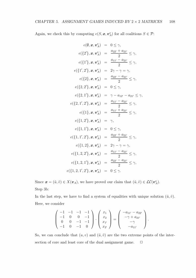
CHAPTER 5. ASSIGNMENT GAMES INDUCED BY 2 × 2 MATRICES 108
Again, we check this by computing e(S, x, v?A) for all coalitions S ∈ P:
e(∅, x, v?A) = 0 ≤ γ,
e({2′}, x, v?A) =
a22′ + a21′
2≤ γ,
e({1′}, x, v?A) =
a11′ − a21′
2≤ γ,
e({1′, 2′}, x, v?A) = 2γ − γ = γ,
e({2}, x, v?A) =
a22′ − a21′
2≤ γ,
e({2, 2′}, x, v?A) = 0 ≤ γ,
e({2, 1′}, x, v?A) = γ − a12′ − a21′ ≤ γ,
e({2, 1′, 2′}, x, v?A) =
a11′ − a21′
2≤ γ,
e({1}, x, v?A) =
a11′ + a21′
2≤ γ,
e({1, 2′}, x, v?A) = γ,
e({1, 1′}, x, v?A) = 0 ≤ γ,
e({1, 1′, 2′}, x, v?A) =
a22′ + a21′
2≤ γ,
e({1, 2}, x, v?A) = 2γ − γ = γ,
e({1, 2, 2′}, x, v?A) =
a11′ − a21′
2≤ γ,
e({1, 2, 1′}, x, v?A) =
a22′ − a21′
2≤ γ,
e({1, 2, 1′, 2′}, x, v?A) = 0 ≤ γ.
Since x = (u, v) ∈ X(vA), we have proved our claim that (u, v) ∈ LC(v?A).
Step 3b:
In the last step, we have to find a system of equalities with unique solution (u, v).
Here, we consider
−1 −1 −1 −1−1 0 0 −10 0 −1 −1−1 0 −1 0
·
x1
x2
x1′
x2′
=
−a11′ − a22′
−γ + a21′
−γ−a11′
.
So, we can conclude that (u, v) and (u, v) are the two extreme points of the inter-
section of core and least core of the dual assignment game. 2
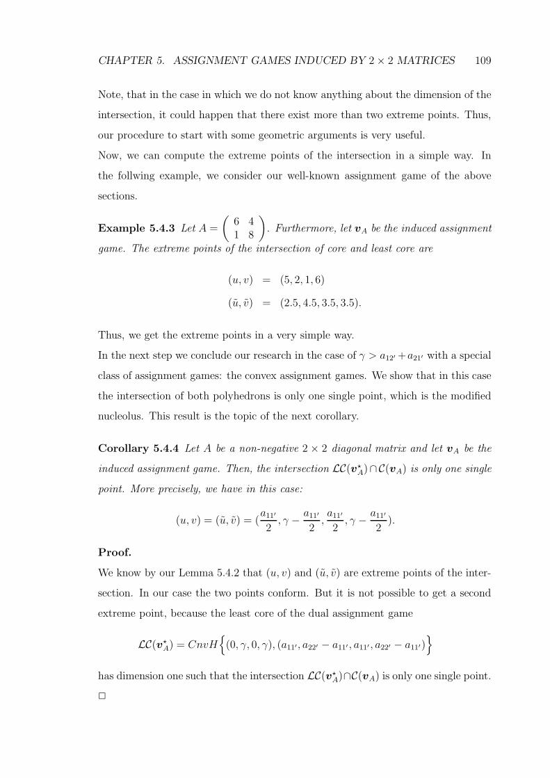
CHAPTER 5. ASSIGNMENT GAMES INDUCED BY 2 × 2 MATRICES 109
Note, that in the case in which we do not know anything about the dimension of the
intersection, it could happen that there exist more than two extreme points. Thus,
our procedure to start with some geometric arguments is very useful.
Now, we can compute the extreme points of the intersection in a simple way. In
the follwing example, we consider our well-known assignment game of the above
sections.
Example 5.4.3 Let A =
(
6 41 8
)
. Furthermore, let vA be the induced assignment
game. The extreme points of the intersection of core and least core are
(u, v) = (5, 2, 1, 6)
(u, v) = (2.5, 4.5, 3.5, 3.5).
Thus, we get the extreme points in a very simple way.
In the next step we conclude our research in the case of γ > a12′ +a21′ with a special
class of assignment games: the convex assignment games. We show that in this case
the intersection of both polyhedrons is only one single point, which is the modified
nucleolus. This result is the topic of the next corollary.
Corollary 5.4.4 Let A be a non-negative 2 × 2 diagonal matrix and let vA be the
induced assignment game. Then, the intersection LC(v?A)∩C(vA) is only one single
point. More precisely, we have in this case:
(u, v) = (u, v) = (a11′
2, γ −
a11′
2,a11′
2, γ −
a11′
2).
Proof.
We know by our Lemma 5.4.2 that (u, v) and (u, v) are extreme points of the inter-
section. In our case the two points conform. But it is not possible to get a second
extreme point, because the least core of the dual assignment game
LC(v?A) = CnvH
{
(0, γ, 0, γ), (a11′, a22′ − a11′ , a11′ , a22′ − a11′)}
has dimension one such that the intersection LC(v?A)∩C(vA) is only one single point.
2
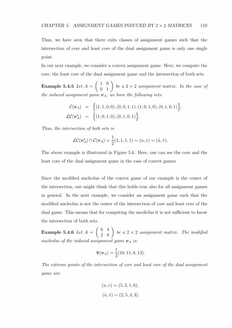
CHAPTER 5. ASSIGNMENT GAMES INDUCED BY 2 × 2 MATRICES 110
Thus, we have seen that there exits classes of assignment games such that the
intersection of core and least core of the dual assignment game is only one single
point.
In our next example, we consider a convex assignment game. Here, we compute the
core, the least core of the dual assignment game and the intersection of both sets.
Example 5.4.5 Let A =
(
1 00 1
)
be a 2 × 2 assignment matrix. In the case of
the induced assignment game vA, we have the following sets:
C(vA) ={
(1, 1, 0, 0), (0, 0, 1, 1), (1, 0, 1, 0), (0, 1, 0, 1)}
,
LC(v?A) =
{
(1, 0, 1, 0), (0, 1, 0, 1)}
.
Thus, the intersection of both sets is
LC(v?A) ∩ C(vA) =
1
2(1, 1, 1, 1) = (u, v) = (u, v).
The above example is illustrated in Figure 5.6. Here, one can see the core and the
least core of the dual assignment game in the case of convex games.
Since the modified nucleolus of the convex game of our example is the center of
the intersection, one might think that this holds true also for all assignment games
in general. In the next example, we consider an assignment game such that the
modified nucleolus is not the center of the intersection of core and least core of the
dual game. This means that for computing the modiclus it is not sufficient to know
the intersection of both sets.
Example 5.4.6 Let A =
(
6 42 8
)
be a 2 × 2 assignment matrix. The modified
nucleolus of the induced assignment game vA is:
Ψ(vA) =1
3(10, 11, 8, 13).
The extreme points of the intersection of core and least core of the dual assignment
game are:
(u, v) = (5, 2, 1, 6),
(u, v) = (2, 5, 4, 3).
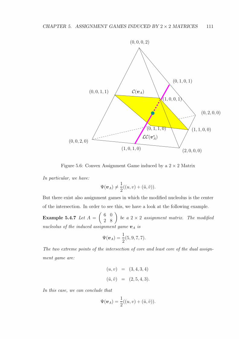
CHAPTER 5. ASSIGNMENT GAMES INDUCED BY 2 × 2 MATRICES 111
(0, 0, 2, 0)
(1, 0, 1, 0) (2, 0, 0, 0)
(1, 1, 0, 0)
(0, 2, 0, 0)
(0, 1, 0, 1)
(0, 0, 0, 2)
(0, 0, 1, 1)
LC(v?A)
C(vA)
(1, 0, 0, 1)
(0, 1, 1, 0)
Figure 5.6: Convex Assignment Game induced by a 2 × 2 Matrix
In particular, we have:
Ψ(vA) 6=1
2((u, v) + (u, v)).
But there exist also assignment games in which the modified nucleolus is the center
of the intersection. In order to see this, we have a look at the following example.
Example 5.4.7 Let A =
(
6 02 8
)
be a 2 × 2 assignment matrix. The modified
nucleolus of the induced assignment game vA is
Ψ(vA) =1
2(5, 9, 7, 7).
The two extreme points of the intersection of core and least core of the dual assign-
ment game are:
(u, v) = (3, 4, 3, 4)
(u, v) = (2, 5, 4, 3).
In this case, we can conclude that
Ψ(vA) =1
2((u, v) + (u, v)).
CHAPTER 5. ASSIGNMENT GAMES INDUCED BY 2 × 2 MATRICES 112
So, we can conclude that it is not sufficient to konw the etreme points of the intersec-
tion of core and least core if we want to compute the modfied nucleolus. Sometimes
the modified nucleolus is the center of the intersection and sometimes it is not. Only
in the case of convex assignment games our procceding yields the modified nucleolus.
Until now, we have focused only on the extreme points for the case γ > a12′ +a21′ . In
the next lemma, we have a look at these extreme points in the case that γ ≤ a12′+a21′
holds true. As in the first case, we find two extreme points of the intersection of
both sets. More precisely, we have:
Lemma 5.4.8 Let A be a non-negative 2 × 2 matrix, such that the induced assign-
ment game vA has a stable core. Furthermore, let a11′ ≤ a22′ and γ ≤ a21′ + a12′.
Then, we have the two extreme points (u, v) and (u, v) of the intersection of the core
and the least core of the dual assignment game:
u1 =a11′
2−
γ
2+
a12′
2,
u2 =3
2γ −
a11′
2−
a12′
2,
v1′ =γ
2−
a12′
2+
a11′
2,
v2′ =γ
2+
a12′
2−
a11′
2,
and
u1 =γ
2−
a21′
2+
a11′
2,
u2 =γ
2+
a21′
2−
a11′
2,
v1′ =a11′
2−
γ
2+
a21′
2,
v2′ =3
2γ −
a11′
2−
a21′
2.
Proof.
The idea of the proof is the same idea as in Lemma 5.4.2. So we have for each
extreme point the following three steps. First, we show that our point (u, v) is an
element of the core. In the second step, we prove that this point is also an element
of the least core of the dual assignment game. Last but not least, we show that
CHAPTER 5. ASSIGNMENT GAMES INDUCED BY 2 × 2 MATRICES 113
(u, v) is an extreme point, that is, it is a solution of a special system of equalities.
After this, we repeat the same steps for the point (u, v).
Step 1a:
By definition,
(u, v) ≥ 0
follows immediately. Furthermore, we have
∑
i∈P
ui +∑
j′∈Q
vj′ = 2γ =∑
i∈P
aii′.
In order to show that (u, v) is an element of the core, we only have to check that
ui + vj′ ≥ aij′
holds for all (i, j′) ∈ P × Q. More precisely, we have the following inequalities:
u1 + v1′ = a11′ ,
u1 + v2′ = a12′ ,
u2 + v1′ = 2γ − a12′ ≥ γ − a12′ ≥ a21′ ,
u2 + v2′ = 2γ − a11′ = a22′ ,
such that we can conclude that (u, v) is an element of the core.
Step 2a:
In this step, we have to check that (u, v) is an element of the least core of the dual
assignment game. Therefore, we have to check that
x = (u, v) ∈ X(vA)
and that
maxS∈P
e(S, x, v?A) = γ (5.4)
holds true. By definition, x ∈ X(vA) follows immediately. The equality (5.4) follows
from the fact that γ ≤ a12′ + a21′ holds.
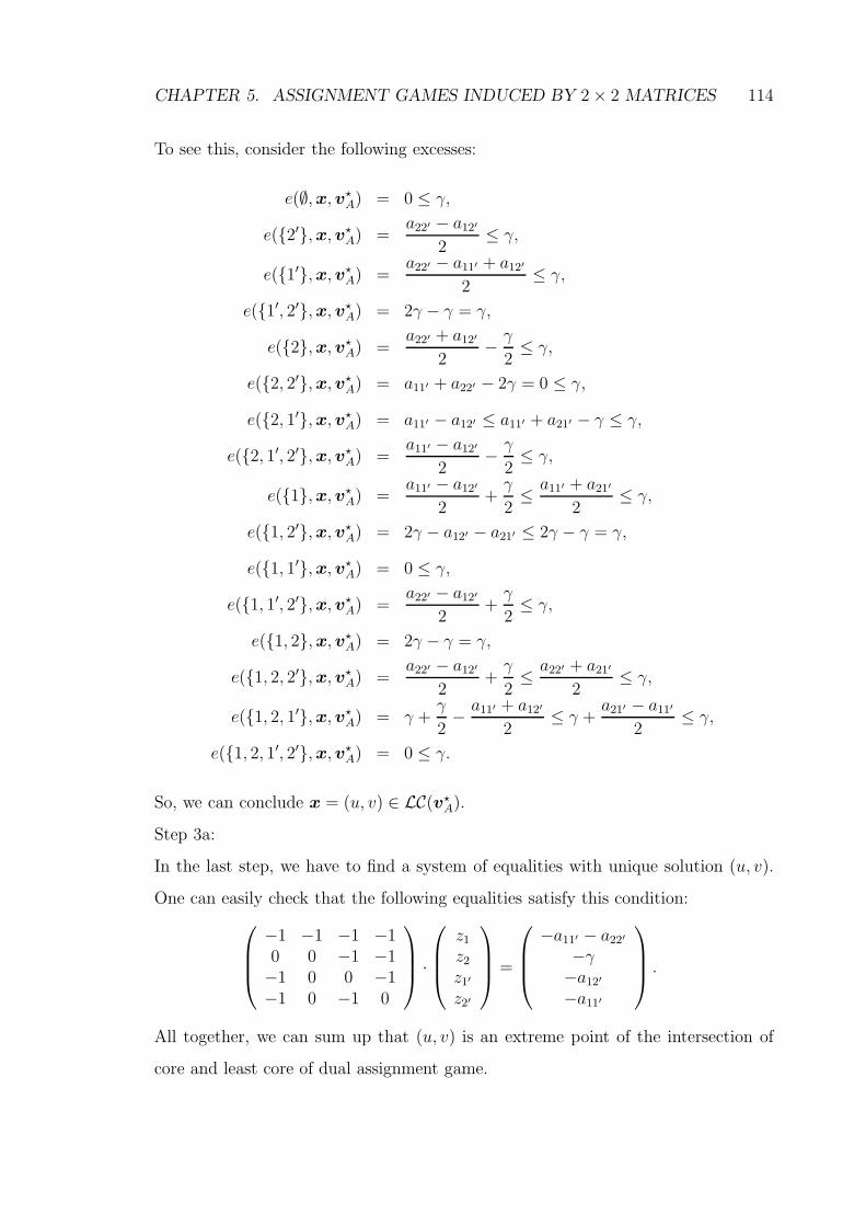
CHAPTER 5. ASSIGNMENT GAMES INDUCED BY 2 × 2 MATRICES 114
To see this, consider the following excesses:
e(∅, x, v?A) = 0 ≤ γ,
e({2′}, x, v?A) =
a22′ − a12′
2≤ γ,
e({1′}, x, v?A) =
a22′ − a11′ + a12′
2≤ γ,
e({1′, 2′}, x, v?A) = 2γ − γ = γ,
e({2}, x, v?A) =
a22′ + a12′
2−
γ
2≤ γ,
e({2, 2′}, x, v?A) = a11′ + a22′ − 2γ = 0 ≤ γ,
e({2, 1′}, x, v?A) = a11′ − a12′ ≤ a11′ + a21′ − γ ≤ γ,
e({2, 1′, 2′}, x, v?A) =
a11′ − a12′
2−
γ
2≤ γ,
e({1}, x, v?A) =
a11′ − a12′
2+
γ
2≤
a11′ + a21′
2≤ γ,
e({1, 2′}, x, v?A) = 2γ − a12′ − a21′ ≤ 2γ − γ = γ,
e({1, 1′}, x, v?A) = 0 ≤ γ,
e({1, 1′, 2′}, x, v?A) =
a22′ − a12′
2+
γ
2≤ γ,
e({1, 2}, x, v?A) = 2γ − γ = γ,
e({1, 2, 2′}, x, v?A) =
a22′ − a12′
2+
γ
2≤
a22′ + a21′
2≤ γ,
e({1, 2, 1′}, x, v?A) = γ +
γ
2−
a11′ + a12′
2≤ γ +
a21′ − a11′
2≤ γ,
e({1, 2, 1′, 2′}, x, v?A) = 0 ≤ γ.
So, we can conclude x = (u, v) ∈ LC(v?A).
Step 3a:
In the last step, we have to find a system of equalities with unique solution (u, v).
One can easily check that the following equalities satisfy this condition:
−1 −1 −1 −10 0 −1 −1−1 0 0 −1−1 0 −1 0
·
z1
z2
z1′
z2′
=
−a11′ − a22′
−γ−a12′
−a11′
.
All together, we can sum up that (u, v) is an extreme point of the intersection of
core and least core of dual assignment game.
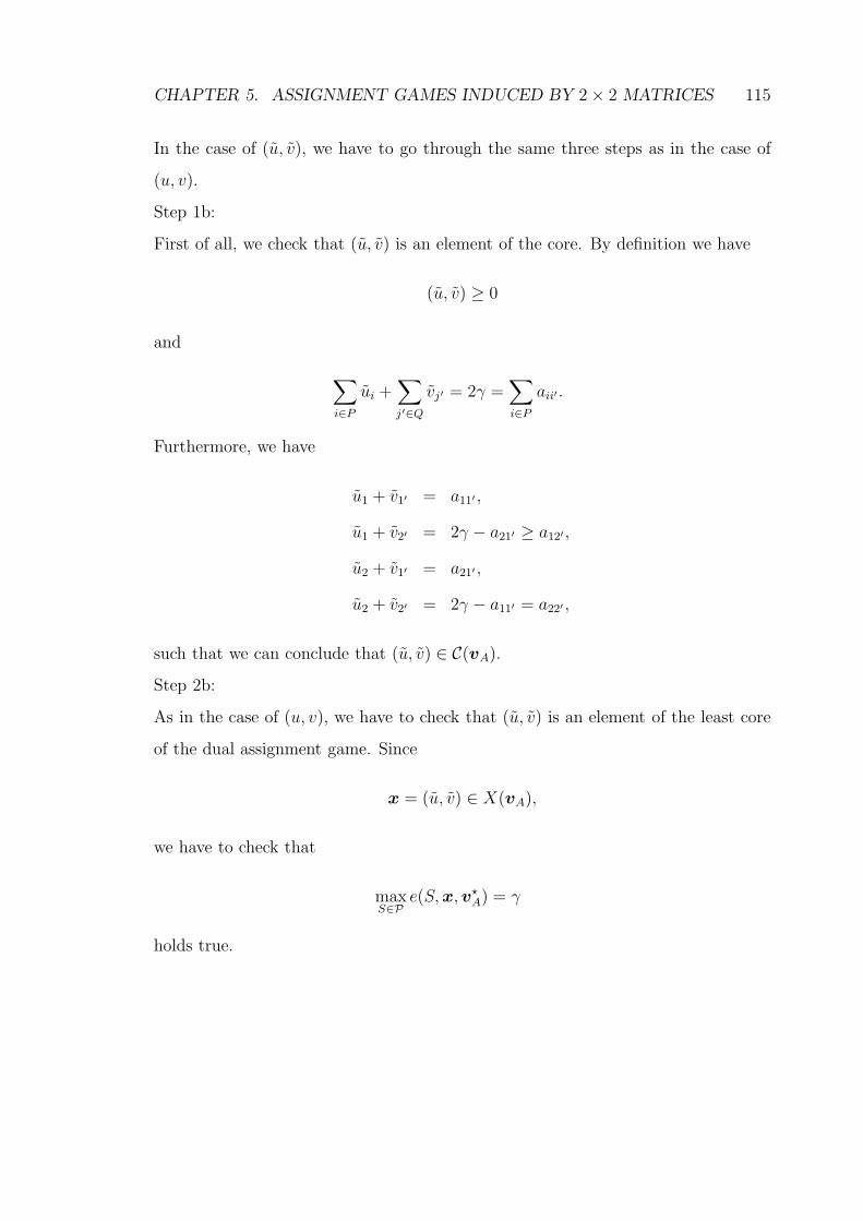
CHAPTER 5. ASSIGNMENT GAMES INDUCED BY 2 × 2 MATRICES 115
In the case of (u, v), we have to go through the same three steps as in the case of
(u, v).
Step 1b:
First of all, we check that (u, v) is an element of the core. By definition we have
(u, v) ≥ 0
and
∑
i∈P
ui +∑
j′∈Q
vj′ = 2γ =∑
i∈P
aii′.
Furthermore, we have
u1 + v1′ = a11′ ,
u1 + v2′ = 2γ − a21′ ≥ a12′ ,
u2 + v1′ = a21′ ,
u2 + v2′ = 2γ − a11′ = a22′ ,
such that we can conclude that (u, v) ∈ C(vA).
Step 2b:
As in the case of (u, v), we have to check that (u, v) is an element of the least core
of the dual assignment game. Since
x = (u, v) ∈ X(vA),
we have to check that
maxS∈P
e(S, x, v?A) = γ
holds true.
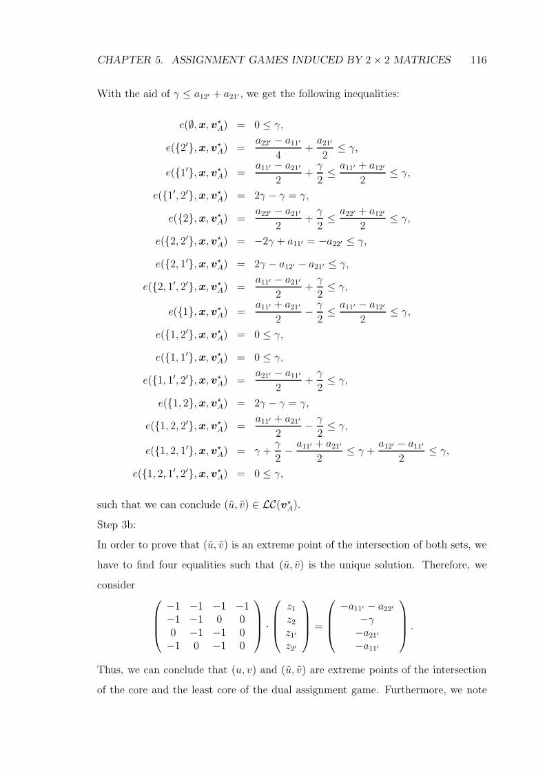
CHAPTER 5. ASSIGNMENT GAMES INDUCED BY 2 × 2 MATRICES 116
With the aid of γ ≤ a12′ + a21′ , we get the following inequalities:
e(∅, x, v?A) = 0 ≤ γ,
e({2′}, x, v?A) =
a22′ − a11′
4+
a21′
2≤ γ,
e({1′}, x, v?A) =
a11′ − a21′
2+
γ
2≤
a11′ + a12′
2≤ γ,
e({1′, 2′}, x, v?A) = 2γ − γ = γ,
e({2}, x, v?A) =
a22′ − a21′
2+
γ
2≤
a22′ + a12′
2≤ γ,
e({2, 2′}, x, v?A) = −2γ + a11′ = −a22′ ≤ γ,
e({2, 1′}, x, v?A) = 2γ − a12′ − a21′ ≤ γ,
e({2, 1′, 2′}, x, v?A) =
a11′ − a21′
2+
γ
2≤ γ,
e({1}, x, v?A) =
a11′ + a21′
2−
γ
2≤
a11′ − a12′
2≤ γ,
e({1, 2′}, x, v?A) = 0 ≤ γ,
e({1, 1′}, x, v?A) = 0 ≤ γ,
e({1, 1′, 2′}, x, v?A) =
a21′ − a11′
2+
γ
2≤ γ,
e({1, 2}, x, v?A) = 2γ − γ = γ,
e({1, 2, 2′}, x, v?A) =
a11′ + a21′
2−
γ
2≤ γ,
e({1, 2, 1′}, x, v?A) = γ +
γ
2−
a11′ + a21′
2≤ γ +
a12′ − a11′
2≤ γ,
e({1, 2, 1′, 2′}, x, v?A) = 0 ≤ γ,
such that we can conclude (u, v) ∈ LC(v?A).
Step 3b:
In order to prove that (u, v) is an extreme point of the intersection of both sets, we
have to find four equalities such that (u, v) is the unique solution. Therefore, we
consider
−1 −1 −1 −1−1 −1 0 00 −1 −1 0−1 0 −1 0
·
z1
z2
z1′
z2′
=
−a11′ − a22′
−γ−a21′
−a11′
.
Thus, we can conclude that (u, v) and (u, v) are extreme points of the intersection
of the core and the least core of the dual assignment game. Furthermore, we note
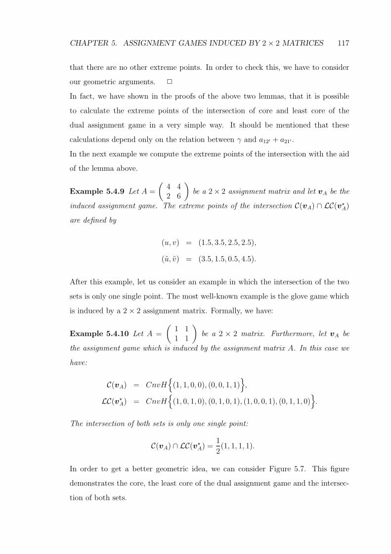
CHAPTER 5. ASSIGNMENT GAMES INDUCED BY 2 × 2 MATRICES 117
that there are no other extreme points. In order to check this, we have to consider
our geometric arguments. 2
In fact, we have shown in the proofs of the above two lemmas, that it is possible
to calculate the extreme points of the intersection of core and least core of the
dual assignment game in a very simple way. It should be mentioned that these
calculations depend only on the relation between γ and a12′ + a21′ .
In the next example we compute the extreme points of the intersection with the aid
of the lemma above.
Example 5.4.9 Let A =
(
4 42 6
)
be a 2× 2 assignment matrix and let vA be the
induced assignment game. The extreme points of the intersection C(vA) ∩ LC(v?A)
are defined by
(u, v) = (1.5, 3.5, 2.5, 2.5),
(u, v) = (3.5, 1.5, 0.5, 4.5).
After this example, let us consider an example in which the intersection of the two
sets is only one single point. The most well-known example is the glove game which
is induced by a 2 × 2 assignment matrix. Formally, we have:
Example 5.4.10 Let A =
(
1 11 1
)
be a 2 × 2 matrix. Furthermore, let vA be
the assignment game which is induced by the assignment matrix A. In this case we
have:
C(vA) = CnvH{
(1, 1, 0, 0), (0, 0, 1, 1)}
,
LC(v?A) = CnvH
{
(1, 0, 1, 0), (0, 1, 0, 1), (1, 0, 0, 1), (0, 1, 1, 0)}
.
The intersection of both sets is only one single point:
C(vA) ∩ LC(v?A) =
1
2(1, 1, 1, 1).
In order to get a better geometric idea, we can consider Figure 5.7. This figure
demonstrates the core, the least core of the dual assignment game and the intersec-
tion of both sets.
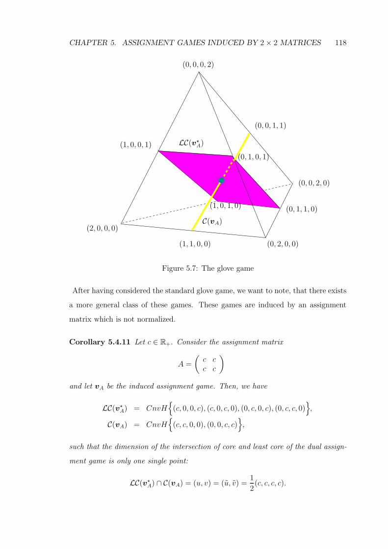
CHAPTER 5. ASSIGNMENT GAMES INDUCED BY 2 × 2 MATRICES 118
(2, 0, 0, 0)
(1, 1, 0, 0) (0, 2, 0, 0)
(0, 1, 1, 0)
(0, 0, 2, 0)
(0, 0, 1, 1)
(0, 0, 0, 2)
(1, 0, 0, 1)
C(vA)
LC(v?A)
(0, 1, 0, 1)
(1, 0, 1, 0)
Figure 5.7: The glove game
After having considered the standard glove game, we want to note, that there exists
a more general class of these games. These games are induced by an assignment
matrix which is not normalized.
Corollary 5.4.11 Let c ∈ R+. Consider the assignment matrix
A =
(
c cc c
)
and let vA be the induced assignment game. Then, we have
LC(v?A) = CnvH
{
(c, 0, 0, c), (c, 0, c, 0), (0, c, 0, c), (0, c, c, 0)}
,
C(vA) = CnvH{
(c, c, 0, 0), (0, 0, c, c)}
,
such that the dimension of the intersection of core and least core of the dual assign-
ment game is only one single point:
LC(v?A) ∩ C(vA) = (u, v) = (u, v) =
1
2(c, c, c, c).
CHAPTER 5. ASSIGNMENT GAMES INDUCED BY 2 × 2 MATRICES 119
Since the modified nucleolus of the game of our example is the center of the intersec-
tion, one might think that this holds true also for all assignment games in general. In
the next example, we consider an assignment game such that the modified nucleolus
is not in the center of the intersection of core and least core of the dual game. This
means that for computing the modiclus it is not sufficient to know the intersection
of both sets.
Example 5.4.12 Let A =
(
6 53 8
)
be a 2 × 2 assignment matrix. The modified
nucleolus of the induced assignment game vA is
Ψ(vA) =1
3(10, 11, 8, 13).
The two extreme points of the intersection of core and least core of the dual assign-
ment game are:
(u, v) = (2, 5, 4, 3)
(u, v) = (5, 2, 1, 6).
In this case, we can conclude that
Ψ(vA) 6=1
2((u, v) + (u, v)).
But there are also assignment games in which the modified nucleolus is the center
of the intersection. In order to see this, we have a look at the following example.
Example 5.4.13 Let A =
(
8 84 10
)
be a 2 × 2 assignment matrix. The modified
nucleolus of the induced assignment game vA is:
Ψ(vA) = (5, 4, 3, 6).
The extreme points of the intersection of core and least core of the dual assignment
game are:
(u, v) =1
2(7, 11, 9, 9),
(u, v) =1
2(13, 5, 3, 15).
In particular, we have:
Ψ(vA) =1
2((u, v) + (u, v)).
Thus, if we want to calculate modiclus we have to find another way.
Chapter 6
Conclusions
In this thesis we provided a basic definition of cooperative game theory with transfer-
able utility including the most well-known solution concepts. Important conditions,
like the strong nullplayer property were shown. In the next step our main inter-
est was on the connections between different solution concepts in the case of the
so-called assignment games. Here, we particularly analyzed the connection between
the Shapley value and the core in the case of exact assignment games. Our main
result in this context is that the Shapley value is an element of the core. For the
direct proof, we needed an alternative description of exact assignment games. In
order to show that exactness is a necessary condition for our theorem, we considered
non-exact assignment games such that the Shapley value is not an element of the
core. But we have also seen that there exists non-exact assignment games such that
the Shapley value is in the core. Next, we made some statements about the mod-
ified nucleolus of an assignment game. In this context, we started by considering
the class of c-convex games which yield the class of dual assignment games. Our
results are very useful since the modified nucleolus is self dual and it is an element
of the least core of the dual assignment game. We found some properties of the least
core of the dual assignment game which can be extended to some special subclasses.
For example in the case of convex assignment games, it is possible to compute the
most important solution concepts, like the core, the Shapley value, the nucleolus,
modiclus and the least core of the dual game. Note that for the calculations, we
only need to use the assignment matrix. Chapter 5 gave a more detailed analysis of
the core and the least core of the dual assignment game in the case of exact assign-
120
CHAPTER 6. CONCLUSIONS 121
ment games which are induced by a 2 × 2 matrix. Since the two polyhedrons have
dimension two, it is possible to gain a more geometrical perspective. In particular,
we generated an image of the intersection of both sets such that we were able to
compute this intersection.
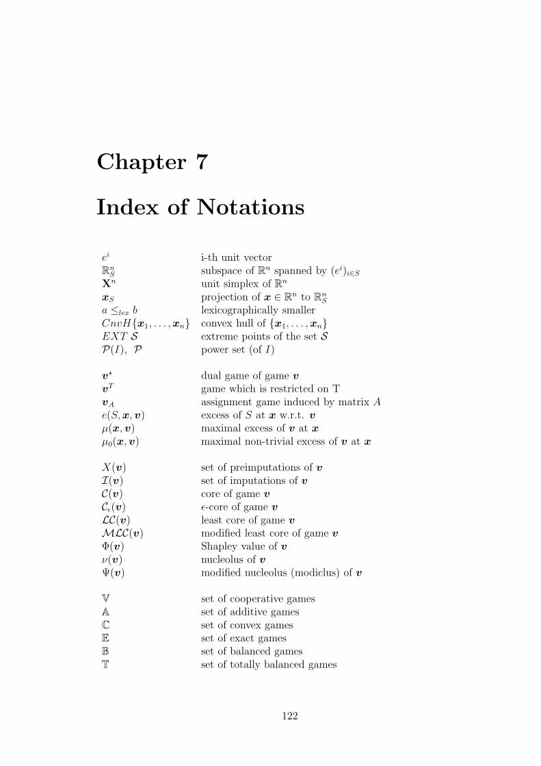
Chapter 7
Index of Notations
ei i-th unit vectorRn
S subspace of Rn spanned by (ei)i∈S
Xn unit simplex of Rn
xS projection of x ∈ Rn to RnS
a ≤lex b lexicographically smallerCnvH{x1, . . . , xn} convex hull of {x1, . . . , xn}EXT S extreme points of the set SP(I), P power set (of I)
v? dual game of game v
vT game which is restricted on TvA assignment game induced by matrix Ae(S, x, v) excess of S at x w.r.t. v
µ(x, v) maximal excess of v at x
µ0(x, v) maximal non-trivial excess of v at x
X(v) set of preimputations of v
I(v) set of imputations of v
C(v) core of game v
Cε(v) ε-core of game v
LC(v) least core of game v
MLC(v) modified least core of game v
Φ(v) Shapley value of v
ν(v) nucleolus of v
Ψ(v) modified nucleolus (modiclus) of v
V set of cooperative gamesA set of additive gamesC set of convex gamesE set of exact gamesB set of balanced gamesT set of totally balanced games
122
Bibliography
[1] Balinski, M. L. and D. Gale (1987): On the Core of the Assignment game, in
Functional Analysis, Optimization and Mathematical Economics, ed. by L. J.
Leifman, Oxford Univ. Press, New York, pp. 274-289.
[2] Bondareva, O. N. (1963): Some applications of linear programming methods to
the theory of cooperative games, in Problemi Kibernitiki 10, pp. 119-139.
[3] Driessen, T. (1988): Cooperative Games, Solutions and Applications, Boston:
Kluwer Academic Publishers.
[4] Gillies, D. B. (1953): Some theorems on n-Person Games, Ph.D. thesis, Prince-
ton University.
[5] Gillies, D. B. (1959): Solutions to General Non-zero-sum games, in Annals of
Mathematics Study, Vol. 40, pp. 47-85.
[6] Hoffmann, M. (2004): Assignment-Games, Diploma Thesis, Bielefeld Univer-
sity.
[7] Hoffmann, M. and P. Sudholter (2007): The Shapley value of exact assignment
games, International Journal of Game Theory, Vol. 35, pp. 557-568.
[8] Inarra, E. and J. M. Usategui (1993): The Shapley Value and Average Convex
Games, in International Journal of Game Theory, Vol. 22, pp. 13-29.
[9] von Neumann, J. and O. Morgenstern (1944): Theory of Games and Economic
Behavior, Princeton: Princeton University Press.
123
BIBLIOGRAPHY 124
[10] Maschler, M.; B. Peleg and L. S. Shapley (1979): Geometric properties of the
kernel, nucleolus, and related solution concepts, in Mathematics of Operations
Research 4, pp. 303-338.
[11] Peleg, B. and P. Sudholter (2003): Introduction to the Theory of cooperative
Games, Boston: Kluwer Academic Publishers.
[12] Raghavan, T. E. S. and P. Sudholter (2005): The Modiclus and Core Stability,
in International Journal of Game Theory, Vol. 33, pp. 467-478.
[13] Rosenmuller, J. (1981): Theory of Games an Markets, North-Holland Publish-
ing Company.
[14] Rosenmuller, J. (2004): Operations Research A: Linear Programming and Bi-
matrix Games, Lecture Notes.
[15] Roth, A. E. and M. A. O. Sotomayor (1990): Two-sided matching: A study in
game-theoretic modeling and analysis, Cambridge University Press, New York,
pp. 202-221.
[16] Schmeidler, D. (1969): The nucleolus of a characteristic function game, in SIAM
Journal on Applied Mathematics 17, pp. 1163-1170.
[17] Schmeidler, D. (1972): Cores of Exact Games, in Journal of Mathematical
Analysis and Applications, Vol. 40, pp. 214-225.
[18] Shapley, L. S. (1953): A value for N-person games, in Annals of Mathematics
Study, Vol. 28, pp. 307-317.
[19] Shapley, L. S. (1967): On balanced sets and cores, in Naval Research Logistics
Quaterly 14, pp. 453-460.
[20] Shapley, L. S. (1971): Cores of convex games, in International Journal of Game
Theory, Vol. 1, pp. 11-26.
[21] Shapley, L. S. and M. Shubik (1963): The core of an economy with nonconvex
preferences, in RM-3518, The Rand Corporation, Santa Monica, CA.
BIBLIOGRAPHY 125
[22] Shapley, L. S. and M. Shubik (1966): Quasi-cores in a monetary economy with
nonconvex preferences, in Econometrica 34, pp. 805-827.
[23] Shapley, L. S. and M. Shubik (1972): The Assignment Game I: The Core, in
International Journal of Game Theory, Vol. 1, pp. 111-130.
[24] Sharkey, W. W. (1982): Cooperative Games with Large Cores, in International
Journal of Game Theory, Vol. 11, pp. 175-182.
[25] Solymosi, T. and T. E. S. Raghavan (1994): An algorithm for finding the
nucleolus of assignment games, in International Journal of Game Theory, Vol.
23, pp. 119-143.
[26] Solymosi, T. and T. E. S. Raghavan (2001): Assignment games with stable
core, in International Journal of Game Theory, Vol. 30, pp. 177-185.
[27] Sudholter, P. (1993): The modified nucleolus of a cooperative game, Habilita-
tion Thesis, University of Bielefeld.
[28] Sudholter, P. (1994): Solution Concepts for C-Convex, Assignment, and M2-
Games, in Institute of Mathematical Economics, Working Paper No. 232, Biele-
feld University.
[29] Sudholter, P. (1996): The modified nucleolus as canonical representation of
weighted majority games, in Mathematics of Operations Research, Vol. 21, pp.
734-756.
[30] Sudholter, P. (1997): The modified nucleolus: Properties and axiomatizations,
in International Journal of Game Theory, Vol. 26, pp. 147-182.
[31] Sudholter, P. (2002): Equal Treatment for Both Sides of Assignment Games in
the Modified Least Core, in Homo Oeconomicus XIX(3), pp. 413-437.


![Assignment 2 Solution[1]](https://img.pdfslide.us/doc/110x75/55cf96c8550346d0338dc126/assignment-2-solution1.jpg)