On simulating the turbulent flow around the Ahmed body: A French–German collaborative evaluation of LES and DES

Computers & Fluids 78 (2013) 10–23

Contents lists available at ScienceDi rect

Computers & Fluids

journal homepage: www.elsevier .com/locate /compfluid

On simulating the turbulent flow around the Ahmed body: A French–Germancollaborative evaluation of LES and DES

Eric Serre a,⇑, Matthieu Minguez b, Richard Pasquetti c, Emmanuel Guilmineau d, Gan Bo Deng d,Michael Kornhaas e, Michael Schäfer e, Jochen Fröhlich f, Christof Hinterberger g, Wolfgang Rodi g

a M2P2 CNRS UMR 6181, Université Aix-Marseille, France b SEAL Engineering, Nîmes, France c Lab. J.-A. Dieudonné, CNRS UMR 6621, Université Nice – Sophia-Antipolis, France d Ecole Centrale de Nantes – CNRS UMR 6598, France e Fachgebiet Numerische Berechnungsverfahren im Maschinenbau, TU Darmstadt, Germany f Institut für Strömungsmechanik, TU Dresden, Germany g Institut für Hydromechanik, Karlsruhe Institute of Technology, Germany

a r t i c l e i n f o a b s t r a c t

Article history: Received 20 December 2010 Received in revised form 5 May 2011 Accepted 31 May 2011 Available online 17 June 2011

Keywords:AerodynamicsFlow around bluff body Large eddy simulation Detached eddy simulation Spectral method

0045-7930/$ - see front matter � 2011 Elsevier Ltd. Adoi: 10.1016/j.compfluid.2011.05.017

⇑ Corresponding author. Tel.: +334 91 11 85 35; faxE-mail address: [email protected] (E. Ser

The paper presents a comp arative analysis of recent simulations, conducted in the framework of a French- Germ an collaboration on LES of Complex Flows, for the so-called Ahmed body at Reynolds number 768000 and slant angle 25 �. It provides a juxtaposition of results obtained with different eddy-resolv ing modeling approache s, i.e. two Large Eddy Simulations (LES) on body-fitted curvilinear grids, a stabilized spectral method and a Detachted Eddy Simulation (DES) on an unstructured grid. The paper presents a comprehen- sive data base including both instantaneous and statistical data. A central achievement is the comparative assessment of the different app roaches with an appreci ation of the respective advantages and disadvan- tages of the various methods. In particular, issues on computational cost and ease of impleme ntation are addressed in addition to the qua lity of results.

� 2011 Elsevier Ltd. All rights reserved.

1. Introduction

The complex interactions between flow separations and the dynamic behavior of the vortex wake govern the aerodynamic forces acting on road vehicles. Detailed knowled ge of these physical mechanism s is required to successfully design future cars. The so-called Ahmed body [1] is a simplified car-shaped body made up of a parallelepip ed with rounded edges at the front and aslanted face at the rear, as displayed in Fig. 1. The flow around this body reproduces the basic aerodynamic features of cars on a well- defined simplified geometry, so that it can be used for the valida- tion of turbulence modeling approaches, conceive d for this type of flow, by comparing numerica l results with well-defined experiments of reference. Modeling this flow still constitutes a challenging task so that it has been chosen as a benchmark case for the ‘‘ERCOFTAC /IAHR Worksho ps on Refined Flow Modelling’’ in 2001 and 2002 [18,25,46] and by the DFG-CNRS program LES of Complex Flows [47].

ll rights reserved.

: +334 91 11 85 02. re).

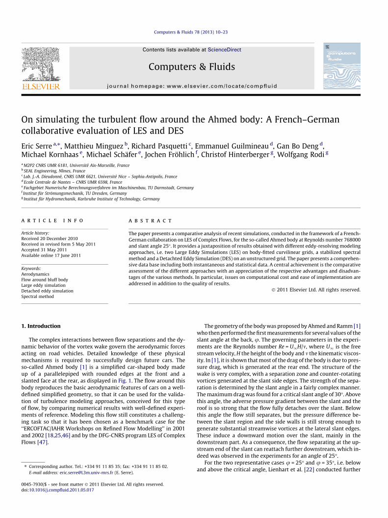
The geometry of the body was proposed by Ahmed and Ramm [1]who then performed the first measure ments for several values of the slant angle at the back, u. The governing parameters in the experiments are the Reynolds number Re = U1H/m, where U1 is the free stream velocity, H the height of the body and m the kinematic viscosity. In [1], it is shown that most of the drag of the body is due to pressure drag, which is generated at the rear end. The structure of the wake is very complex, with a separation zone and counter-rotating vortices generated at the slant side edges. The strength of the separation is determined by the slant angle in a fairly complex manner. The maximum drag was found for a critical slant angle of 30 �. Above this angle, the adverse pressure gradient between the slant and the roof is so strong that the flow fully detaches over the slant. Below this angle the flow still separates, but the pressure difference between the slant region and the side walls is still strong enough to generate substantial streamwise vortices at the lateral slant edges. These induce a downward motion over the slant, mainly in the downstre am part. As a consequence, the flow separating at the upstream end of the slant can reattach further downstream , which indeed was observed in the experiments for an angle of 25 �.

For the two representat ive cases u = 25 � and u = 35 �, i.e. below and above the critical angle, Lienhart et al. [22] conducted further

http://dx.doi.org/10.1016/j.compfluid.2011.05.017

mailto:[email protected]

http://dx.doi.org/10.1016/j.compfluid.2011.05.017

http://www.sciencedirect.com/science/journal/00457930

http://www.elsevier.com/locate/compfluid

Fig. 1. Side, rear and top view of the Ahmed body together with the coordinate system used. Distances are in mm. The slant angle u = 25 � in the current analysis.

E. Serre et al. / Computers & Fluids 78 (2013) 10–23 11

experiments with the same body and recovered the general observations of Ahmed. This study provided well-defined LDA measurements of mean velocity fields and turbulence statistics at Re = 768,000 that are used as reference in the present study.

In the literature, a certain number of studies are now available for the two angles 25 � and 35 � of the rear slanted surface using different turbulence modeling approaches. Several of these employed Reynolds-Average d Navier–Stokes (RANS) models such as [10,6,4,29,1 2] . A review on this topic by F. Menter can be found in [25]. The cited studies used a large variety of two-equatio n models, from the standard K � �model with wall-functio n to the K �x ap-proaches including an algebraic treatment of the Reynolds tensor (EARSM), and also more sophisticated Reynolds Stresses Models. The overall conclusion is that while the simulations were relatively successful in predicting the 35 � case, they did not provide satisfactory results for the 25 � case. Indeed, for u = 25 � the shear due to the partial detachment of the flow on the upper part of the slant provides small scale structures, related to a Kelvin–Helmholtz instability, which significantly increase the momentum transfer across the mean streamlin es and enhance the three-dim ensionality as well as the unsteadiness of the flow. This type of mechanism is very difficultto model by RANS approaches so that the predictions at subcritical angle generally remain unsatisfa ctory whatever turbulence model is used. Most of the RANS simulatio ns miss the flow separation at the rear part or, when they accurately predict the separation onset, they fail in the massively separated flow regions containing many coherent structures by mainly underpredictin g the level of turbulent stresses [25].

The above remarks suggest that LES may constitute a valuable way to compute the flow around the Ahmed body, particular ly for subcritical slant angles. The first LES results [16] using a geometry without bottom wall and the Smagorinsky model globally cap- tured the topology of the flow for a subcritical slant angle u = 28 �but drag estimation and flow field visualizations were characteri s- tics of a flow for u > 30 �. Several LES studies [13,14,32,21] showedthat the accuracy of the solution is undeniably improved compared to the RANS studies. Particularly, the unsteady phenomena are well described and the solutions almost capture the peak of turbulent kinetic energy measure d at the beginning of the slant.

A fundamenta l problem with LES, however, is the need to resolve the turbulent boundary layer along the roof of the body which is decisive for adequately capturing the separated shear layer over the slant. Due to the high Reynolds number it is extre- mely thin with d � 10 mm or d/L � 10�2, as illustrate d in Fig. 11 be-low. Even if a wall function approach is used as in [13,14], the usual resolution requirements in streamw ise and spanwise direction can

hardly be met. This can impact the resolved turbulent motion in the shear layer and deteriorate the solution quality.

For this reason, hybrid LES/RANS methods have been applied as well to this flow. The overall strategy with such an approach is to model the attached turbulent boundary layer in RANS manner while LES-type resolution of the large-scale turbulent wake is at- tempted. Several concepts of hybridizatio n between LES and RANS exist, as detailed in [8]. In particular , one can distinguish between segregated approaches, where a sharp interface between a steady RANS and an unsteady LES is used so that the computed solution is discontinuo us there, and unified approaches where the computed solution is continuous througho ut. The latter inevitably leads to a gray zone between the LES and the RANS region. The most prominent unified hybrid approach is Detached Eddy Simula- tion (DES) proposed by Spalart et al. [39]. Indeed, the DES of Men- ter and Kuntz [29,30] and Kapadia et al. [20] show globally much better results than the ones provided by RANS approach es. They resolve in particular for u = 25 � the vortical structures in the wake as well as in the shear layer between the freestream and the recirculation but do not recover the partial detachment on the slant. Mathey and Cokljat [27] presented results for an approach close to segregated modeling. They performed a RANS simulation for the entire flow and then added an LES domain which starts right at the corner of the slant where the flow separates and covers the wake region. The inflow condition s for this subdomain were generate d from the mean flow of the RANS solution to which syn- thesized turbulence was superimposed to an amount specified by the RANS solution and generate d by means of a vortex method [26]. The coupling back to the RANS domain, which distinguishe san LES with particular inflow conditions from a truly hybrid simulation, is still missing in this paper, but the results presented show the quality of the solution which can be achieved with this approach. Indeed, the obtained statistical data capture the measurements very well. Unified approaches on the other hand, if not employin g some type of stochastic forcing, rely on the instabilit yof the mean flow in the transition between upstream RANS and downstre am LES region. For the Ahmed body this effect is quite strong so that substantial unsteady motion is created which in turn can yield results closer to the experiment than those obtained with (U) RANS methods.

The test case of this paper is the one initially defined in 2001 during the 9th ERCOFTAC Workshop on Refined Turbulence Model- ling [46] for a body with subcritical slant angle u = 25 � at aReynolds number of Re = 768,000 (note that in [1] the Reynolds number is based on the length of the body). Measurem ents were performed by Lienhart and Becker [22,23].

12 E. Serre et al. / Computers & Fluids 78 (2013) 10–23

Two French and two German groups participated in the test calculations and the common analysis (listed in random order):

1. M. Minguez, R. Pasquett i and E. Serre from the Universities of Aix–Marseille and Nice–Sophia-Antipolis (acronym AM-NS).

2. E. Guilmineau and G.B. Deng from Ecole Centrale de Nantes (acronym ECN).

3. M. Kornhaas and M. Schäfer from the Technica l University of Darmstadt (acronym TUD).

4. C. Hinterberger , J. Fröhlich1 and W. Rodi from the University of Karlsruhe, now Karlsruhe Institute of Technology (acronym KIT).

The overall effort for this collaborative assessment was substantial since each individual group simulated this complex high-Rey- nolds number flow until converged statistics were obtained and comparative analyzes were carried out in the sequel.

The results reported below were achieved with one DES and three different LES methods developed in the four research teams:

� KIT: LES with a Smagorin sky subgrid scale model in which the near-wall energy-c ontaining motions are not resolved but modeled by wall-function (LES-NWM hereafter);� TUD: LES with near-wall resolution using a dynamic Smagorin-

sky model (LES-NWR hereafter);� AM-NS: High-order LES based on spectral approximation s stabi-

lized by spectral vanishing viscosity (LES-SVV hereafter);� ECN: Detached Eddy Simulation k �x SST (DES-SST hereafter).

The comparis on of the results obtained with these approach es allows to illustrate both the effects of the near-wal l resolution and subgrid-scale modeling, using similar accuracy for the numerical schemes (LES-NWM, LES-NWR and DES-SST), as well as the effect of a more accurate resolution of the large scales structures by comparing LES-SVV with the others. While discussing here the flow around the Ahmed body, the conclusions drawn certainly also apply to other bluff body flows or high Reynolds number flowswith massive separation.

The present paper is organized as follows. The computational setup is presented in Section 2. Section 3 briefly outlines the physical models and the discretiza tion schemes adopted by each group. The performanc e of the different numerical approaches is bench- marked in Section 4 through direct comparisons of the most relevant statistical and instantaneo us data. Finally, conclusions from this study are drawn in Section 5.

Table 1Boundary conditions used in the four simulations.

Simulation Inlet Outlet Sides Ground Top Body

DES-SST U1 Pressure Slip No-slip Slip No-slip LES-NWR U1 Convective Slip No-slip Slip No-slip LES-NWM U1 Convective Slip Wall Slip Wall

2. Computationa l setup

The geometry of the car model conforms with the experiments of Lienhart et al. [22]. The Ahmed body, of length L = 1044 mm, height H = 288 mm, and width W = 389 mm, is placed at d = 50 mm from the ground (Fig. 1) and is mounted in a 3/4 open test section (floor, but no side walls or ceiling). The u = 25 � slantangle configuration is considered in the current analysis. The wind tunnel model was suspended by four stilts. This was also ac- counted for in the simulations, except in the simulatio n LES-SVV where these are disregarded while still positioning the body at the same height.

The computational domain is X = 8L � 5W � 5H, as defined in the ERCOFTAC benchma rk. This implies a blocking factor, definedas the ratio between the cross section of the bluff body and channel cross section, equal to 4.24%. For the LES-SVV simulation the domain size was however slightly reduced to X = 8L � 3.5W � 3.5H(blocking factor 8.24%) in order to save computational cost. In

1 At the time the project ran this autho r worked in Karlsr uhe.

Minguez et al. [32], the two-poin t correlations, nearly equal to zero in spanwise direction, have shown that this computational domain width is large enough to avoid a confinement effect. The bluff body is located at the distance 2L from the inlet.

The free stream velocity of the measure ments was U1 = 40 m/s so that the Reynolds number based on the height of the body H isRe = 768000. It is of the same order of magnitud e but somewhat lower than the one, Re = 1.2 � 106, used in the original experiment of Ahmed and Ramm [1].

The flow is assumed to be governed by the filtered Navier–Stokes equations for incompres sible fluids. In primitive variables they read

@tU þ U:rU ¼ �rpþ mDU þr:sSGS ð1Þr:U ¼ 0; ð2Þ

where t is time, p the pressure divided by the density q and U thevelocity vector with component s (u,v,w) in streamwise (x), vertical (y) and spanwise (z) directions, respective ly. The term sSGS repre-sents the subgrid-sc ale stresses, and the usual overbar designi ng fil-tered quantities is dropped throug hout here. In the following , L, U1and L/U1 define the charac teristic length, speed and time, respectively. In dimensio nless form, m is the inverse of the Reynolds number Re. Eqs. (1), (2) are imposed over the computa tional domain Xfor the time interval (0,T). At t = 0 the fluid is at rest.

Boundary conditions are summarized in Table 1. At the inflowsection, uniform laminar velocity u = U1 is imposed. At the outlet, a convective boundary condition

@t/þ Uc@x/ ¼ 0 ð3Þ

where / = u, v, w is used with Uc = U1, or a pressure conditio n is imposed. The latter amount s to impose a value for the pressure together with vanishing normal gradien t of the velocity component s.

In the spanwise direction all the approaches consider slip surfaces on both sides, except LES-SVV where this direction is assumed to be homogeneous in order to use Fourier expansion yielding a solution which is periodic in z. Note that for LES of turbulent flow slip and periodicity are different conditions since sym- metries of the statistics do not carry over to the instantaneo us resolved fluctuations. In the present scenario, however , the flowis steady and laminar at the sides of the computational domain since steady laminar flow is imposed at the inlet and no turbulence is generate d remote from the body and the bottom wall, so that effectively both conditions are equal in that case.

In all simulations the velocity vector was imposed to vanish at solid walls, but for LES-SVV the Ahmed body is modeled by using the penalizat ion technique described in [32]. It amounts to introduce a force term, at the right hand side of (1), equal to a O(1/Dt) negative constant (Dt being the time-step) times the velocity inside the obstacle and zero outside, driving any non-zero velocity to zero inside the obstacle. The equations enhanced in this way are solved throughout, in X and inside the obstacle, so that the boundary condition on the surface of the obstacle is imposed indirectly and in a weaker sense, compared to the finite volume methods .With LES-NWM a wall function approach was employed, as

function function LES-SVV U1 Convective Periodic No-slip Slip Penalization


detailed below, to reduce the number of degrees of freedom and by not fully resolving the wall boundary layers.

3. Physical models and discretiz ations

In this Section, the different numerical approaches and computational codes are briefly outlined. They are summarized in Table 2,where the numerical degrees of freedom characterizi ng the benchmark calculation are presented. Three of the four approaches are based on second-order finite volume schemes, while the fourth is a spectral scheme.

3.1. LES with Smagorinsky model and wall function (LES-NWM)

This simulation was performed with the finite volume Code LESOCC2 (Large Eddy Simulation On Curvilinear Coordinates ) [15]which is an enhanced and fully-paral lelized version of the code LE- SOCC [2]. It uses body-fitted curvilinear block-structured grids with second-order central differenc es for the discretizatio n of the convective and the viscous fluxes. Time advancement is accomplis hed by an explicit predictor–corrector scheme. The predictor is a low-stor- age three-ste p second order Runge–Kutta method. Conservation of mass is achieved in the corrector step by the solution of a pressure correction equation employing the ILU-type SIP procedure [43].The momentum- interpolation method of Rhie and Chow [36] isemployed to prevent pressure–velocity decoupling and associated oscillations.

The Smagorinsky eddy-viscosi ty model [38] relates the subgrid- scale eddy viscosity lt to the strain rate of the resolved motion Sij

to generate a velocity scale and to the mesh size as a length scale by

mt ¼ C2s D

2jSj; ð4Þ

where the filter width D is determine d as the cubic root of the volume of the computa tional cell. The value Cs = 0.13 was chosen for the model coefficient. It is larger than used in other simulation sbut was found to be necessary here in order to avoid numerica linstabili ties. Finally, a wall function similar to the Werner-W engle approach [45] was used: The universal law of the wall is assumed to hold instantaneo usly betwee n the wall-adjacent grid point and the wall, but in contrast to [45], the latter was represented by seven logarithm ic segment s fitted to DNS data from turbulent channe lflow [15]. This was applied at the walls of the vehicle and at the bottom of the channel.

It should be mentioned that the wall models cited are basically developed for attached flows. Their applicati on in separated flowregions may seem questionable. As a matter of fact, however , the wall shear stress in these regions is comparatively small so that such models operate in the range of low y+-values. According to the results of [44] obtained for the hill flow, the sensitivit y of the

Table 2Summary of numerical meth odologies. Nomenclature used in this table is as follows: (i) FloBDF2/3 = second/third order backward Euler, CN = implicit Crank–Nicolson, RK2/4 = secon

Simulation (group) Numerical method (code)

Time scheme (dimensionlesstime-step [L/U1])

Subgrid-scale model

DES-SST (ECN) FV2 (ISIS-CFD) BDF3 (9.5 � 10�3)

k �x SST [29]

LES-NWR (TUD) FV2 (FASTEST) CN (2.3 � 10�5) Dynamic Smagorinsky

LES-NWM (KIT) FV2 (LESOCC2)

RK2 (1.3 � 10�4) Smag. (Cs = 0.13) + wall function model

LES-SVV (AM-NS) PS (SVVLES) BDF2-RK4 (2.3 � 10�3)

SVV

flow with respect to the wall model in a recirculation zone seems low.

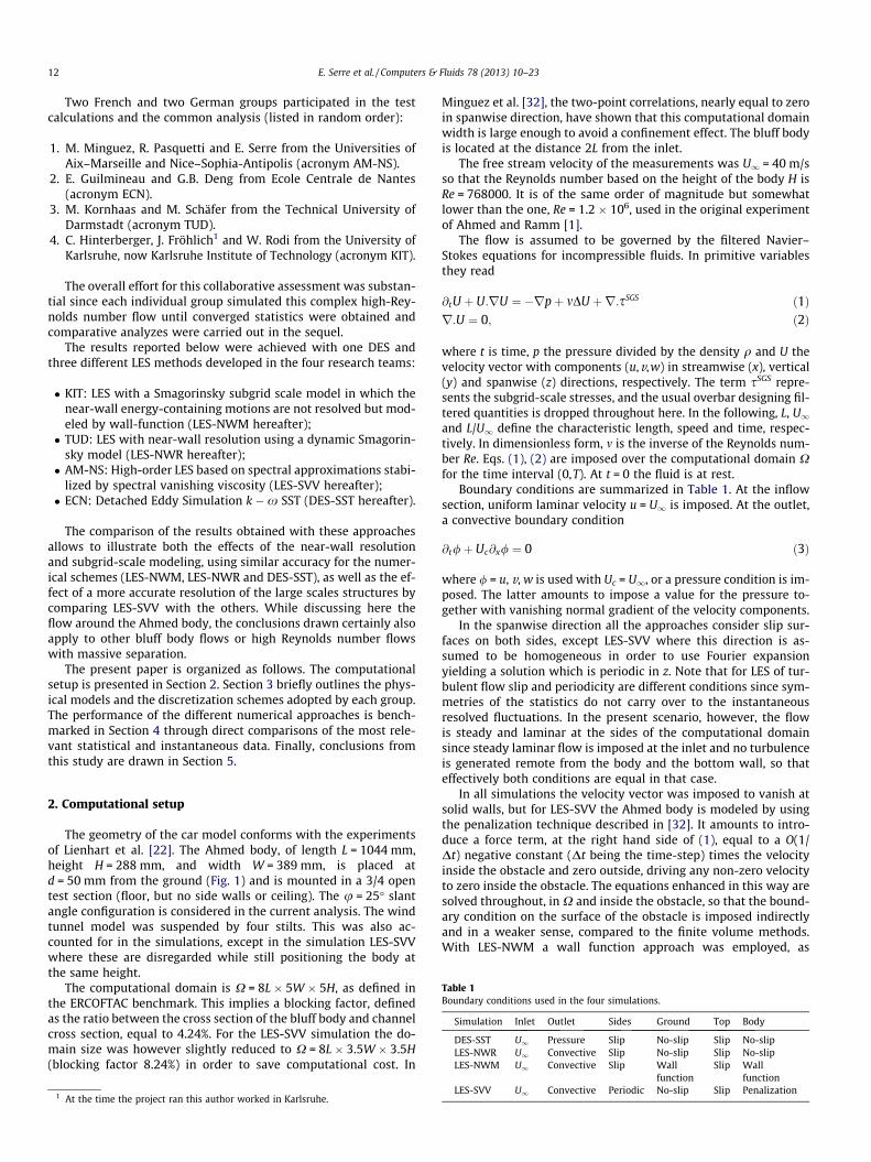
The grid used for LES-NWM (Fig. 2) was generate d with the commerc ial software ICEM-CFD and consists of 214 blocks and 18.5 � 106 cells. It has an O-grid structure around the body and further away, which is necessary due to the rounded front. Grid points were clustered in the region of the slant, especiall y close to the top and side edges. Consequently, the near-wall cell center has a wall distance of about 40 wall units on the average, but it varies from approximat ely 10 in the separated regions along the slant back to 150 close to the top rear edge. The spanwise and streamw ise extent of the grid cells is up to a factor of 10 larger, except in the refinement regions close to the edges. Later experi- ences with wall functions showed that as a rule of thumb the spanwise step size of the grid should equal the wall-normal step size [7]. This could not be achieved here for reasons of computational cost.

3.2. Wall-resolving LES with dynamic Smagorinsky model (LES-NWR)

Simulations were performed with the code FASTEST [5], ahighly efficient parallel flow solver using boundary fitted, block structure d hexahedral grids. Convective and diffusive fluxes are approximat ed with second-order central differencing schemes .The implicit second-order Crank-Ni colson scheme is applied for time discretiza tion. Pressure–velocity coupling is realized by means of a SIMPLE-type algorithm which is embedded in a geometric multi-grid scheme with standard restriction and prolonga- tion [3]. The resulting linear systems are solved with the SIP method.

As for LES-NWM, the Smagorinsky eddy-viscosi ty model was employed associated here with the dynamic determination of the model coefficient Cg ¼ C2

s proposed by Germano et al. [9] and Lilly [24]. The model coefficient is determined for each SIMPLE iteration when computin g the new time level tn+1. To obtain a smooth behavior of Cg and to avoid its well known oscillations, a relaxation of the computed value C�g in time with the factor b 2 [0, 1] and its value from the previous time step at tn is carried out

C��g ð~x; tnþ1Þ ¼ ð1� bÞC�gð~x; tnÞ þ bC�gð~x; tnþ1Þ; ð5Þ

as proposed in [2]. Unphy sical behavi or and numerical instabilities, are removed by clipping negative values of Cg. Furthermor e, an upper bound of Cg is introduce d to make sure that the model does not becom e too diffusive so that finally

Cgð~x; tnþ1Þ ¼min max fC��g ;0g;1n o

; ð6Þ

with the correspon ding eddy viscosity

mt ¼ CgD2jSj: ð7Þ

w solvers : FV2 = second-orde r finite volume, PS = pseudo-spectr al. (ii) Time integration :d/forth-order Rung e Kutta.

Points in mesh [10 6points](near-wall point)

Memory (GB)

Averaging time [L/U1] (s)

CPU time (h)

23 (y+6 1) 46 35 (0.92) 20000 IBM P4 (64

procs)40 (y+ � 1) 80 1 (0.027) 5000 IBM P6 (32

procs)18.5 (y+ � 40) 37 4.5 (0.12) 30000 IBM SP (128

procs)21.3 (y+ � 400) 18 11 (0.29) 500 Nec SX8 (8

procs)

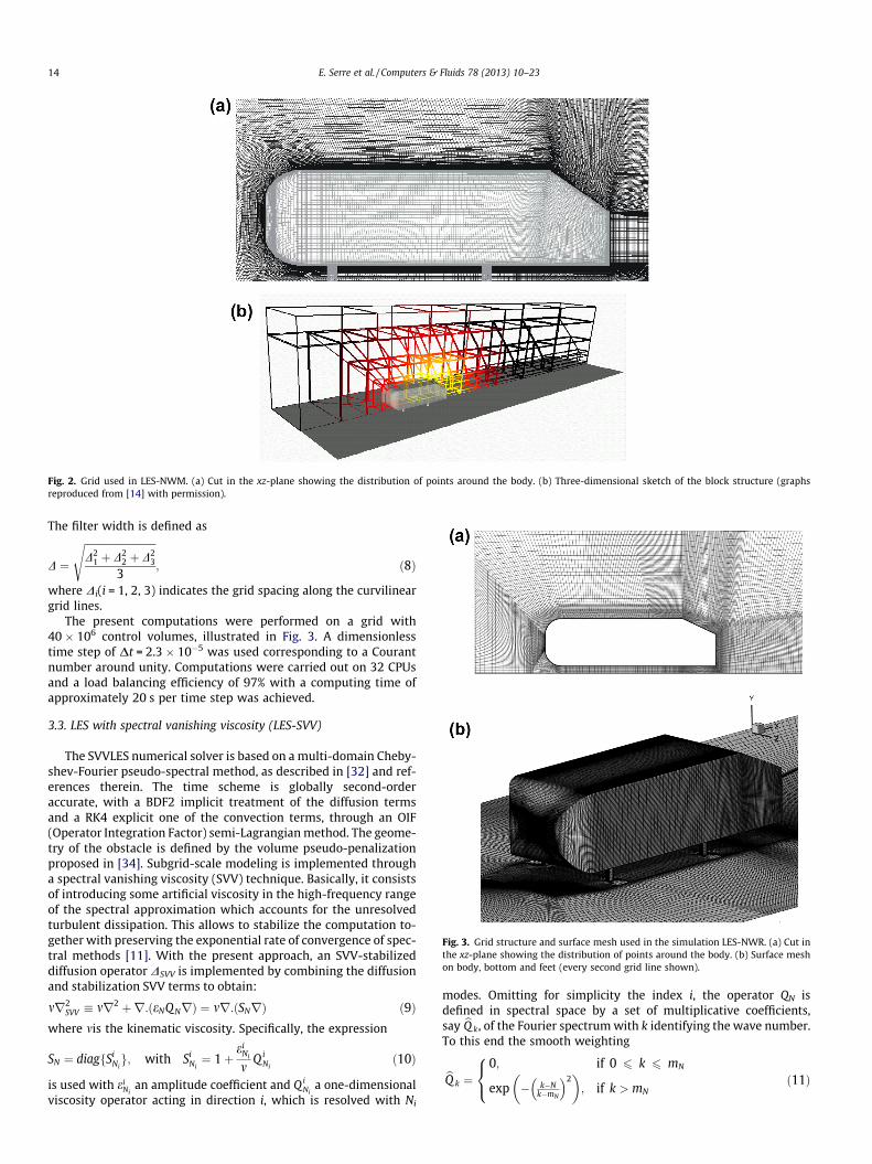
Fig. 2. Grid used in LES-NWM. (a) Cut in the xz-plane showing the distribution of points around the body. (b) Three-dimensional sketch of the block structure (graphsreproduced from [14] with permission).

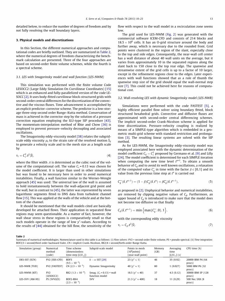
Fig. 3. Grid structure and surface mesh used in the simulation LES-NWR. (a) Cut in the xz-plane showing the distribution of points around the body. (b) Surface mesh on body, bottom and feet (every second grid line shown).


The filter width is defined as

D ¼

ffiffiffiffiffiffiffiffiffiffiffiffiffiffiffiffiffiffiffiffiffiffiffiffiffiffiffiffiD2

1 þ D22 þ D2

3

3

s; ð8Þ

where Di(i = 1, 2, 3) indicate s the grid spacing along the curvilinear grid lines.

The present computations were performed on a grid with 40 � 106 control volumes, illustrated in Fig. 3. A dimensio nless time step of Dt = 2.3 � 10�5 was used correspond ing to a Courant number around unity. Computati ons were carried out on 32 CPUs and a load balancing efficiency of 97% with a computing time of approximat ely 20 s per time step was achieved.

3.3. LES with spectral vanishing viscosity (LES-SVV)

The SVVLES numerical solver is based on a multi-doma in Cheby- shev-Fourier pseudo-spectra l method, as described in [32] and references therein. The time scheme is globally second-o rder accurate, with a BDF2 implicit treatment of the diffusion terms and a RK4 explicit one of the convection terms, through an OIF (Operator Integration Factor) semi-Lagrangi an method. The geometry of the obstacle is defined by the volume pseudo-penaliz ation proposed in [34]. Subgrid-s cale modeling is implemented through a spectral vanishing viscosity (SVV) technique. Basically, it consists of introducing some artificial viscosity in the high-frequency range of the spectral approximat ion which accounts for the unresolved turbulent dissipation. This allows to stabilize the computation together with preservin g the exponential rate of convergence of spectral methods [11]. With the present approach, an SVV-stabilized diffusion operator DSVV is implemented by combining the diffusion and stabilization SVV terms to obtain:

mr2SVV � mr2 þr:ðeNQ NrÞ ¼ mr:ðSNrÞ ð9Þ

where mis the kinemati c viscosity. Specifically, the expression

SN ¼ diagfSiNig; with Si

Ni¼ 1þ

eiNi

mQ i

Nið10Þ

is used with eiNi

an amplitud e coefficient and QiNi

a one-dimension al viscosity operator acting in direction i, which is resolved with Ni

modes . Omitting for simplic ity the index i, the operator QN isdefined in spectral space by a set of multiplica tive coefficients, say bQ k, of the Fourier spectrum with k identifying the wave number. To this end the smooth weighting

bQ k ¼0; if 0 6 k 6 mN

exp � k�Nk�mN

� �2� �

; if k > mN

8<: ð11Þ

Fig. 4. LES-SVV Grid in the centerplane (xy) illustrating the distribution obtained by non-linear mappings. The subdomain boundaries of the pseudo-spectral multi-domain decomposition are located in regions of clustered grid points. Every grid line is plotted, but only part of the domain is shown.


is used. Hence, all wave numbers below the threshold mN are left unchanged while the higher frequencies are damped . The same procedure is applied to the Chebyshev modes, just identifying k withthe polynom ial degree of the basis function.

The SVV stabilized Laplacian DSVV makes use of mN ¼ffiffiffiffiNp

andeN = 1/ N, independently of the spatial (x,y,z) direction. Within the boundary layer, improvements of the results have however been obtained by using a SVV operator DBL

SVV , with an anisotropic thres- holding as proposed in [32] with mN ¼ f2

ffiffiffiffiffiffiNxp

;5ffiffiffiffiffiffiNy

p;4

ffiffiffiffiffiffiNzpg and

again eN = 1/ N. This is appropriate here as the dominating boundary layers are oriented in x-direction, so that these are covered appropriate ly. Moreove r, nonlinear mappings are used to accumulate grid points at the body boundary.

The solver is parallelized using the MPI library and optimized for a NEC SX8 vector-para llel computer. The computational domain is decomposed into eight sub-domains in streamwise direction. With- in each subdomain the space discretizatio n is Ni = {40, 190, 170}, in the streamwise, vertical and spanwise direction, respectively, so that the resulting grid contains approximat ely 21 � 106 points.Fig. 4 provides a close up of their distribution around the body. Note that the distribut ion of points in the vertical direction has been changed with respect to the usual Chebyshev distribution by aone-dimensi onal non-linear mapping to accumulate grid points near the roof and the slant of the body. Despite this, and due to the treatment of the bluff body by the penalizat ion technique the LES- SVV simulatio ns do not resolve the boundary layers over the Ahmed body. Indeed, the spacing of collocatio n points in streamwise, wall normal and lateral direction is of the order of 400, 80, and 400 wall units, respectivel y. The dimensionless time step used in the simulation LES-SVV was Dt = 2.3 � 10�3 and the required CPU time about 9 s for one time step, i.e. approximat ely 10 �7 s per time step and degree of freedom. Globally, the computations required about 500 CPU hours and the fine grid calculations about 18 GB of memory.

3.4. Detached Eddy Simulation (DES-SST)

The numerical solver ISIS-CFD [35], developed at the Ecole Cent- rale de Nantes, is based on a second-order finite volume method. All flow variables are stored at the geometric center of arbitrarily shaped cells. Volume and surface integrals are evaluated with second-order accurate approximat ions. The face-based method is generalized to two-dimensi onal or three-dimens ional unstructured meshes for which non-overlap ping control volumes are bounded by an arbitrary number of constituti ve faces. Numerical fluxes are reconstructed on cell faces by linear extrapolation of the integrand from the neighboring cell centers. A centered scheme is used for the diffusion terms, whereas for the convective fluxes,the Gamma Differencing Scheme [19] is employed for the present study. Through a Normalized Variable Diagram analysis, this scheme enforces local monoton icity and a convectio n boundedness criterion. The pressure equation is obtained in the spirit of Rhie and Chow [37]. Momentum and pressure equations are solved in a segregated manner as in the SIMPLE coupling procedure [17]. The temporal discretization is fully implicit and second-order accurate.

The DES-SST method is a unified LES/RANS hybrid [8] in which the properties of the grid define the separation of the domain into anear-wal l region where RANS equations are solved and the remain- der where LES equations are solved, i.e. the filtered Navier–Stokesequation s together with a subgrid-scale model. The distinction between the two sets of equations is only done by the source term in the transport equation for a turbulence quantity. DES was first proposed based on the Spalart–Allmaras one equation RANS model [39]. The idea of DES can however be extended to any specific turbulence model [42] and a combinati on with the SST model exists [30] which is now briefly recalled. The DES modification in the SST model is applied to the dissipation term in the equation for the turbulent kinetic energy K. In the SST RANS model it reads [28]

e ¼ b�Kx; ð12Þ

where e is the dissip ation rate and b⁄ a constant of the SST model. For the DES-SST, this term is replaced with

e ¼ FDESb�Kx ð13Þ

where

FDES ¼maxLt

CDESD;1

� �: ð14Þ

In these equations , D is the maximum local grid spacing defined as D = max{ Dx,Dy,Dz}, while Lt is the turbule nt length scale, Lt ¼

ffiffiffiffiKp

=ðb�xÞ and CDES a model constant. In the initial version of DES-SST [30], CDES was 0.61. With the ISIS-CFD solver, the value 0.78 later proposed in [31] is used.

The mesh is generated using HEXPRESS TM, an automatic unstructured mesh generator. This software generates meshes containing only hexahedrons. The computati onal grid used for the present simulatio n consists of 23.1 Mio cells with 384,090 ele- ments to describe the Ahmed body. A first box includes the Ahmed body and the wake until Lx = 5L. The mesh of this box is uniform and the size of each edge is 5 mm. The rear slant, the base of the model and the near wake are immersed in a new box that has auniform mesh and the length of the edge is 1.8 mm. Fig. 5 showsthe mesh in the symmetr y plane. The resolution achieved in this manner is (100 < Dx+ < 134,0.32 < Dy+ < 0.50,90 < Dz+ < 200) and (13 < Dx+ < 110, 0.07 < Dy+ < 0.55,30 < Dz+ < 160) over the roof and the slant, respectively , where x, y, z refer to the local streamwise, wall normal and lateral coordinate.

The dimensionless time step used for this simulation is Dt = 9.5 � 10�3, which correspond s to about 10 3 time steps for one passage of the car at freestream velocity.

3.5. Computin g times

With unsteady simulatio n approaches such as LES and hybrid LES/RAN S methods , statistical data are obtained from computing the unsteady solution using a relatively small time step over a suf- ficient laps of time and then averaging in time and possibly over homogen eous directions . The present geometry does not feature any homogeneous direction, so that only averaging in time was

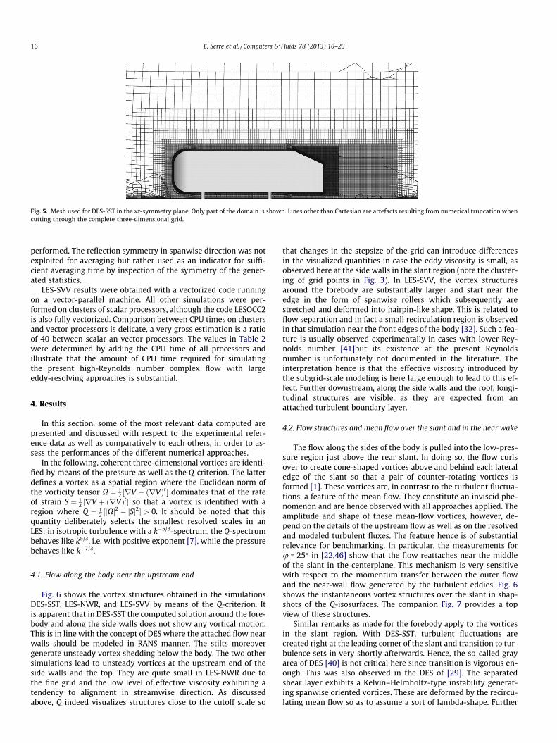
Fig. 5. Mesh used for DES-SST in the xz-symmetry plane. Only part of the domain is shown. Lines other than Cartesian are artefacts resulting from numerical truncation when cutting through the complete three-dimensional grid.


performed. The reflection symmetry in spanwise direction was not exploited for averaging but rather used as an indicator for suffi-cient averaging time by inspection of the symmetry of the generated statistics.

LES-SVV results were obtained with a vectorized code running on a vector-pa rallel machine. All other simulations were performed on clusters of scalar processors, although the code LESOCC2 is also fully vectorized. Comparison between CPU times on clusters and vector processors is delicate, a very gross estimation is a ratio of 40 between scalar an vector processors. The values in Table 2were determined by adding the CPU time of all processors and illustrate that the amount of CPU time required for simulating the present high-Reyno lds number complex flow with large eddy-resolvi ng approaches is substantial.

4. Results

In this section, some of the most relevant data computed are presented and discussed with respect to the experimental reference data as well as comparative ly to each others, in order to as- sess the performances of the different numerical approach es.

In the following, coherent three-dimensio nal vortices are identified by means of the pressure as well as the Q-criterion. The latter defines a vortex as a spatial region where the Euclidean norm of the vorticity tensor X ¼ 1

2 ½rV � ðrVÞt � dominates that of the rate of strain S ¼ 1

2 ½rV þ ðrVÞt � so that a vortex is identified with aregion where Q ¼ 1

2 ½jXj2 � jSj2� > 0. It should be noted that this

quantity deliberately selects the smallest resolved scales in an LES: in isotropic turbulence with a k�5/3-spectrum, the Q-spectrumbehaves like k5/3, i.e. with positive exponent [7], while the pressure behaves like k�7/3.

4.1. Flow along the body near the upstream end

Fig. 6 shows the vortex structure s obtained in the simulations DES-SST, LES-NWR, and LES-SVV by means of the Q-criterion. It is apparent that in DES-SST the computed solution around the forebody and along the side walls does not show any vortical motion. This is in line with the concept of DES where the attached flow near walls should be modeled in RANS manner. The stilts moreover generate unsteady vortex shedding below the body. The two other simulations lead to unsteady vortices at the upstream end of the side walls and the top. They are quite small in LES-NWR due to the fine grid and the low level of effective viscosity exhibiting atendency to alignmen t in streamwise direction. As discussed above, Q indeed visualizes structures close to the cutoff scale so

that changes in the stepsize of the grid can introduce differenc es in the visualized quantities in case the eddy viscosity is small, as observed here at the side walls in the slant region (note the cluster- ing of grid points in Fig. 3). In LES-SVV, the vortex structures around the forebody are substantially larger and start near the edge in the form of spanwise rollers which subsequent ly are stretched and deformed into hairpin-like shape. This is related to flow separation and in fact a small recirculation region is observed in that simulatio n near the front edges of the body [32]. Such a feature is usually observed experimentally in cases with lower Rey- nolds number [41]but its existence at the present Reynolds number is unfortun ately not documented in the literature. The interpretati on hence is that the effective viscosity introduce d by the subgrid-sca le modeling is here large enough to lead to this effect. Further downstream, along the side walls and the roof, longi- tudinal structures are visible, as they are expected from an attached turbulent boundary layer.

4.2. Flow structures and mean flow over the slant and in the near wake

The flow along the sides of the body is pulled into the low-pressure region just above the rear slant. In doing so, the flow curls over to create cone-shaped vortices above and behind each lateral edge of the slant so that a pair of counter-rotati ng vortices is formed [1]. These vortices are, in contrast to the turbulent fluctua-tions, a feature of the mean flow. They constitute an inviscid phe- nomenon and are hence observed with all approaches applied. The amplitud e and shape of these mean-flow vortices, however, depend on the details of the upstream flow as well as on the resolved and modeled turbulent fluxes. The feature hence is of substanti al relevance for benchmarki ng. In particular, the measure ments for u = 25 � in [22,46] show that the flow reattaches near the middle of the slant in the centerpla ne. This mechanism is very sensitive with respect to the momentum transfer between the outer flowand the near-wal l flow generated by the turbulent eddies. Fig. 6shows the instantaneous vortex structure s over the slant in shap- shots of the Q-isosurfa ces. The companion Fig. 7 provides a top view of these structure s.

Similar remarks as made for the forebody apply to the vortices in the slant region. With DES-SST, turbulent fluctuations are created right at the leading corner of the slant and transition to turbulence sets in very shortly afterwards. Hence, the so-called gray area of DES [40] is not critical here since transition is vigorous enough. This was also observed in the DES of [29]. The separated shear layer exhibits a Kelvin–Helmholtz-type instability generat- ing spanwise oriented vortices. These are deformed by the recircu- lating mean flow so as to assume a sort of lambda-shap e. Further

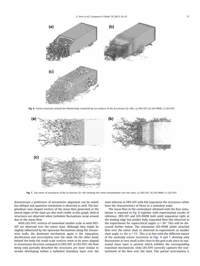
Fig. 6. Vortex structures around the Ahmed body visualized by iso-surfaces of the Q-criterion (Q = 60): (a) DES-SST, (b) LES-NWR, (c) LES-SVV.

Fig. 7. Top views of isosurfaces of the Q-criterion (Q = 60) showing the vortex development over the slant: (a) DES-SST, (b) LES-NWR, (c) LES-SVV.


downstream a preference of streamw ise alignment can be noted, but oblique and spanwise orientation is observed as well. The lon- gitudinal cone-shaped vortices of the mean flow generated at the lateral edges of the slant are also well visible in this graph. Helical structures are observed when turbulent fluctuations wrap around due to the mean flow.

With LES-SVV, vortices of somewhat smaller scale as with DES- SST are observed over the entire slant. Although they might be slightly influenced by the upstream fluctuations along the streamwise walls, the dominant mechanism again is the separation, deceleration and recirculati on over the slant. On the other hand, behind the body the small-scale vortices seem to be more aligned in streamw ise direction compare d to DES-SST. In LES-SVV, the flowbeing only partially detached the structures are more similar to streaks developing within a turbulent boundary layer over the

slant whereas in DES-SST with full separation the structures rather have the characteri stics of those in a turbulent wake.

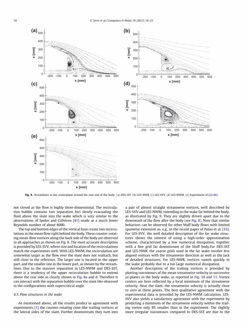
The mean flow in the centerplane obtained with the four simulations is reported in Fig. 8 together with experimental results of reference. DES-SST and LES-NWM both yield separation right at the leading edge but predict fully separated flow like observed in the experiments for supercritical angles u > 30 �. This will be discussed further below. The simulatio n LES-NWR yields attached flow over the entire slant as observed in experiments at smaller slant angle, i.e. for u < 15 �. This is in line with the different nature of the unsteady vortex structure s in Figs. 6 and 7 showing only fluctuations at very small scales close to the grid scale since no separated shear layer is present which exhibits the correspond ing transition mechanism s. Only LES-SVV correctly captures the reattachmen t of the flow over the slant. This partial recirculati on is

(a) (b)

x [mm]

z [m

m]

-200 -100 0 100 200 300 400 500 6000

100

200

300

400

500

(c)

x [mm]

z [m

m]

-200 -100 0 100 200 300 400 500 6000

100

200

300

400

500(d)

(e)

x [mm]

z [m

m]

-200 -100 0 100 200 300 400 500 6000

100

200

300

400

500

z [m

m]

0

100

200

300

400

500

z [m

m]

0

100

200

300

400

500

x [mm]-200 -100 0 100 200 300 400 500 600

x [mm]-200 -100 0 100 200 300 400 500 600

Fig. 8. Streamlines in the centerplane around the rear end of the body: (a) DES-SST, (b) LES-NWR, (c) LES-SVV, (d) LES-NWM, (e) Experiment of [22,46].


not closed as the flow is highly three-dimens ional. The recirculation bubble contains two separation foci slowly evacuating the fluid above the slant into the wake which is very similar to the observations of Spohn and Gilliéron [41] made at a much lower Reynolds number of about 8000.

The top and bottom edges of the vertical base create two recirculations in the mean flow right behind the body. These counter-rotating mean-flow vortices along the back side of the body are observed in all approaches as shown on Fig. 8. The most accurate description is provided by LES-SVV, where size and location of the recirculations match the experiments well. With LES-NWM, the recirculation are somewhat larger as the flow over the slant does not reattach, but still close to the reference. The larger one is located in the upper part, and the smaller one in the lower part, as shown by the streamlines. Due to the massive separation in LES-NWM and DES-SST, there is a tendency of the upper recirculati on bubble to extend above the rear side as clearly shown in Fig. 8a and d. Therefore it can interact with the separation bubble over the slant like observed in the configurations with supercrit ical angle.

4.3. Flow structures in the wake

As mentioned above, all the results predict in agreement with experiments [1] the counter-rotati ng cone-like trailing vortices at the lateral sides of the slant. Further downstream they turn into

a pair of almost straight streamwise vortices, well described by LES-SVV and LES-NWM, extending in the wake far behind the body, as illustrated by Fig. 9. They are slightly driven apart due to the downwa sh of the flow after the body (see Fig. 8). Note that similar behaviors can be observed for other bluff body flows with limited spanwise extension as, e.g., in the recent paper of Palau et al. [33].For LES-SVV, the well detailed description of the far wake structures shows the interest of using a high-order approximat ion scheme, characterized by a low numerical dissipation, together with a fine grid far downstre am of the bluff body.For DES-SST and LES-NWR , the coarse grids used in the far wake involve less aligned vortices with the streamwise direction as well as the lack of detailed structures. For LES-NWR , vortices vanish quickly in the wake probably due to a too large numerical dissipation.

Another description of the trailing vortices is provided by plotting isocontours of the mean streamwise velocity in successive yz-planes in the body wake, as reported in Fig. 10 and 11 . Vortex centers are here reflected by a local minimum of the streamwise velocity. Near the slant, the streamwise velocity is actually close to zero at these points. The best qualitative agreement with the experime ntal data is provided by the LES-NWM calculation. LES- SVV also yields a satisfactory agreement with the experiment by predictin g a minimum of the streamwise velocity within the trailing vortex only 8% smaller than in the experiment. The slightly more irregular isocontour s compared to DES-SST are due to the

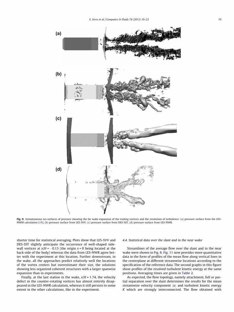
Fig. 9. Instantaneous iso-surfaces of pressure showing the far wake expansion of the trailing vortices and the resolution of turbulence: (a) pressure surface from the LES- NWM calculation [15], (b) pressure surface from LES-SVV, (c) pressure surface from DES-SST, (d) pressure surface from LES-NWR.


shorter time for statistical averaging. Plots show that LES-SVV and DES-SST slightly anticipate the occurrence of well-shap ed side- wall vortices at x/H = �0.13 (the origin x = 0 being located at the back-side of the body) whereas the data from LES-NWR agree better with the experiment at this location. Further downstream , in the wake, all the approaches predict relatively well the locations of the vortex centers but overestimate their size, the solutions showing less organized coherent structures with a larger spanwise expansion than in experime nts.

Finally, at the last station in the wake, x/H = 1.74, the velocity defect in the counter-rotating vortices has almost entirely disap- peared in the LES-NWR calculation, whereas it still persists to some extent in the other calculations, like in the experiment.

4.4. Statistica l data over the slant and in the near wake

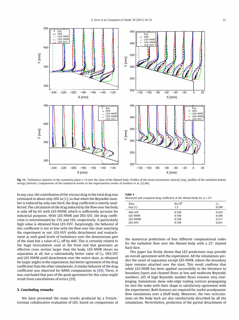
Streamlines of the average flow over the slant and in the near wake were shown in Fig. 8. Fig. 11 now provides more quantitative data in the form of profiles of the mean flow along vertical lines in the centerplane at different streamw ise locations according to the specification of the reference data. The second graphs in this figureshow profiles of the resolved turbulent kinetic energy at the same positions . Averaging times are given in Table 2.

As expected , the flow topology, namely attachment, full or partial separation over the slant determines the results for the mean streamw ise velocity component hui and turbulent kinetic energy K which are strongly interconnected . The flow obtained with

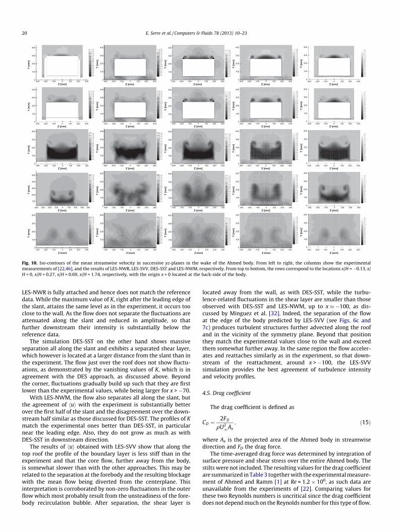
Fig. 10. Iso-contours of the mean streamwise velocity in successive yz-planes in the wake of the Ahmed body. From left to right, the columns show the experimental measurements of [22,46], and the results of LES-NWR, LES-SVV, DES-SST and LES-NWM, respectively. From top to bottom, the rows correspond to the locations x/H = �0.13, x/H = 0, x/H = 0.27, x/H = 0.69, x/H = 1.74, respectively, with the origin x = 0 located at the back-side of the body.


LES-NWR is fully attached and hence does not match the reference data. While the maximum value of K, right after the leading edge of the slant, attains the same level as in the experiment, it occurs too close to the wall. As the flow does not separate the fluctuations are attenuated along the slant and reduced in amplitud e, so that further downstream their intensity is substantially below the reference data.

The simulation DES-SST on the other hand shows massive separation all along the slant and exhibits a separated shear layer, which however is located at a larger distance from the slant than in the experiment. The flow just over the roof does not show fluctu-ations, as demonstrated by the vanishing values of K, which is in agreement with the DES approach , as discussed above. Beyond the corner, fluctuations gradually build up such that they are firstlower than the experimental values, while being larger for x > �70.

With LES-NWM, the flow also separates all along the slant, but the agreement of hui with the experime nt is substantially better over the first half of the slant and the disagreement over the downstream half similar as those discussed for DES-SST. The profiles of Kmatch the experimental ones better than DES-SST, in particular near the leading edge. Also, they do not grow as much as with DES-SST in downstream direction.

The results of hui obtained with LES-SVV show that along the top roof the profile of the boundary layer is less stiff than in the experiment and that the core flow, further away from the body, is somewhat slower than with the other approach es. This may be related to the separation at the forebody and the resulting blockage with the mean flow being diverted from the centerplane. This interpretation is corroborated by non-zero fluctuations in the outer flow which most probably result from the unsteadiness of the forebody recirculation bubble. After separation, the shear layer is

located away from the wall, as with DES-SST, while the turbulence-relate d fluctuations in the shear layer are smaller than those observed with DES-SST and LES-NWM, up to x � �100, as discussed by Minguez et al. [32]. Indeed, the separation of the flowat the edge of the body predicted by LES-SVV (see Figs. 6c and 7c) produces turbulent structures further advected along the roof and in the vicinity of the symmetry plane. Beyond that position they match the experimental values close to the wall and exceed them somewhat further away. In the same region the flow acceler- ates and reattaches similarly as in the experiment, so that downstream of the reattachmen t, around x > �100, the LES-SVV simulatio n provides the best agreement of turbulence intensity and velocity profiles.

4.5. Drag coefficient

The drag coefficient is defined as

CD ¼2FD

qU21Ax

; ð15Þ

where Ax is the projecte d area of the Ahmed body in streamwise direction and FD the drag force.

The time-averag ed drag force was determined by integrati on of surface pressure and shear stress over the entire Ahmed body. The stilts were not included. The resulting values for the drag coefficientare summari zed in Table 3 together with the experimental measure -ment of Ahmed and Ramm [1] at Re = 1.2 � 106, as such data are unavailabl e from the experiments of [22]. Comparing values for these two Reynolds numbers is uncritical since the drag coefficientdoes not depend much on the Reynolds number for this type of flow.

−240 −220 −200 −180 −160 −140 −120

300

350

400

450

X [mm]

Y [m

m]

Exp.DESLES−NWRLES−NWMLES−SVV

−120 −100 −80 −60 −40 −20 0 20200

250

300

350

400

450

X [mm]

Y [m

m]


−240 −220 −200 −180 −160 −140 −120

300

350

400

450

X [mm]

Y [m

m]


−120 −100 −80 −60 −40 −20 0 20200

250

300

350

400

450

X [mm]

Y [m

m]


Fig. 11. Turbulence statistics in the symmetry plane z = 0 over the slant of the Ahmed body. Profiles of the mean streamwise velocity (top), profiles of the turbulent kinetic energy (bottom). Comparisons of the numerical results to the experimental results of Lienhart et al. [22,46].

Table 3Measured and computed drag coefficient of the Ahmed body for u = 25 �.

Data Re/106 CD

Exp [1] 1.2 0.298

DES-SST 0.768 0.343 LES-NWR 0.768 0.346 LES-NWM 0.768 0.317 LES-SVV 0.768 0.431


In any case, the contribution of the viscous drag to the total drag was estimated to about only 20% in [1], so that when the Reynolds number is reduced by only one third, the drag coefficient is merely unaf- fected. The calculation of the drag induced by the flow over the body is only off by 6% with LES-NWM, which is sufficiently accurate for industrial purposes . With LES-NWR and DES-SST, the drag coeffi-cient is overestimat ed by 15% and 16%, respectively . A particular ly high value is obtained from LES-SVV. Surprisingly , the behavior of this coefficient is not in line with the flow over the slant matching the experiment or not. LES-SVV yields detachment and reattach- ment as well good levels of turbulence over the downstream part of the slant but a value of CD off by 44%. This is certainly related to the huge recirculation zone at the front end that generates an effective cross section larger than the body. LES-NWR shows no separation at all, but a substantially better value of CD. DES-SST and LES-NWM yield detachment over the entire slant, as obtained for larger angles in the experiment, but better agreement of the drag coefficient than the other simulations . A similar behavior of the drag coefficient was observed for RANS computations in [29]. There, it was concluded that part of the good agreement for this value might result from cancellations of errors [29].

5. Concluding remarks

We have presented the main results produced by a French–German collaborativ e evaluation of LES, based on comparisons of

the numerical predictions of four different computational codes for the turbulent flow over the Ahmed body with a 25 � slantedback-face.

This paper has firstly shown that LES predictions may provide an overall agreement with the experiment. All the simulations predict the onset of separation except LES-NWR, where the boundary layer remains attached over the slant. This result confirms that while LES-NWR has been applied successfu lly in the literature to boundary layers and channel flows at low and moderate Reynolds numbers , LES of high Reynolds number flows remains very challenging. Simulations show side-edge trailing vortices propagat ing far into the wake with their shape in satisfactory agreement with the experiments. Both features are required for useful aerodynamic flow simulations over a bluff body. Moreove r, the two recirculations on the body back are also satisfactorily described by all the simulatio ns. Nevertheles s, prediction of the partial detachment of


the mean flow over the slant continues to pose a substanti al chal- lenge to these methods, this feature being only obtained in the LES- SVV simulation. The developmen t of attached or separated flowover the slant is strongly connected to the incoming boundary layer over the roof and to the presence and intensity of side edge vortices which drive the fluid of the shear layer towards the slant. The weaker these vortices are, the more defined vortices led to the separation of the boundary layer. According to Fig. 11 , the overestimation of the turbulence intensity at the edge of the slant within the boundary layer could explain that the flow remains attached to the slant in LES-NWR . Moreover, too strong side edge vortices can enhance this behavior.

Some discrepancies between LES-NWM and DES-SST results could be explained by differences in mesh resolution and effective viscosity introduce d by the subgrid-sca le modeling. In both trans- verse and streamw ise direction, over the body the DES-SST grid is coarser than the LES-NWM one. On the contrary to LES-NWM, amesh too much refined at the wall, in normal direction, could be for DES-SST the reason of a transition from URANS to LES, deep in the boundary layer, that could artificially induce a non-physical separation weakening too much the side wall vortices. Indeed, plots of the function FDES show that the switch from URANS to LES occurs at values of the normal wall coordinate y+ � 10. . .30over the roof and y+ � 8. . .10 over the slant.

In the LES-SVV approach, the numerical dissipation may be ne- glected due to the high accuracy of the method. As a consequence, the sub-grid scale dissipation is solely associated to the sub-grid scale modeling introduced through the spectral vanishing viscosity. The main drawback of the LES-SVV prediction is the existence of a confined recirculation at the body front involving turbulent structures further advected along the roof in the vicinity of the symmetry plane and finally delaying the detachment of the boundary over the slant. Such a recirculati on zone at the front generates also an effective cross section larger than the body, thus involving adramatical overestimation of 44% of the drag coefficient. Such arecirculation being only documented experime ntally at much lower Reynolds numbers [41], it can be related to extra local dissipation around the body due a too coarse discretization and/or to the penalization technique. Surprisingly , the values for the drag coefficient have not shown a strong sensitivit y to the flow details since all the other computati ons only slightly overestimate the drag coefficient, with a deviation from the experimental value between around 6–16%.

This paper has also shown that simulatio ns of such three- dimensional unsteady turbulent flow remain costly for LES. All these LES approach es require efficient parallel solvers running on supercompute rs, involving vector processor s as used for LES-SVV or cluster architectures, as used for the other simulations . With mesh sizes of tens of million points converged statistics require per processor more than 200 CPU hours per processor on a cluster and around 60 h on vector computer , which is, per processor , more powerful but also more costly. DES-SST saves computin g time, due to the moderate costs of the RANS model in the boundary layer region. This has allowed longer computations than in the other simulations. On the contrary, the dynamic Smagorin sky procedure, associated with the high resolution required within the boundary layers, has drastically limited the computed time of LES-NWR.

In conclusion, the Ahmed-body test case still today challenges all components of an LES solver. Flow separation, large-scale eddy- ing turbulent structures that dominate the turbulent transport, unsteady processes such as vortex shedding, and transition from laminar to turbulent flow which can happen in various ways, indeed make this flow very challenging for the LES and DES solvers. Nevertheles s, this investigatio n makes certain that LES is the right level of modeling for all flows with similar features and in this sense makes also our results valuable for other bluff bodies flows

at high Reynolds number. Pushing forward LES to a reliable tool for turbulence simulations in practically relevant flows will require neverthe less the improvement of the currently available algo- rithms in terms of accuracy and of cost reduction . Besides, present results confirm that methods based on LES/RANS coupling like DES or zonal approach represent an attractive alternative, even if grid generation can be much more complicated than for a simple RANS or LES case due to the RANS-LES switch.

Acknowled gments

The French authors acknowledge financial support from CNRS through the DFG-CNRS network. The German authors acknowledge financial support by DFG through the research program ‘‘LES of Complex Flows’’ FOR 507. E. Serre acknowledges support from Spanish government through research project FIS2008-01126 .The groups AM-NS and ECN were granted access to the HPC resource s of CINES and IDRIS under the allocation s 2009-0242 and 2010-0129, respectively , by GENCI (Grand Equipement National de Calcul Intensif). The group KIT was attributed CPU time at the Karlsruhe Computer Center SCC.

References

[1] Ahmed SR, Ramm G. Salient features of the time-averaged ground vehicle wake. SAE-Paper 840300; 1984.

[2] Breuer M, Rodi W. Large eddy simulation of complex turbulent flows of practical interest. In: Hirschel EH, editor. Flow simulation with high performance computers II. Notes on numerical fluid mechanics, 52. Braunchweig: Vieweg; 1996. p. 258–74.

[3] Briggs WL, Van Emden H, McCormick SF. A multigrid tutorial. SIAM; 2000. [4] Craft TJ, Gant SE, Iacovides H, Launder BE, Robinson CME. Computational study

of flow around the Ahmed car body (case 9.4). In: 9th ERCOFTAC/IAHR workshop on refined turbulence on modelling, Darmstadt University of Technology, Germany; 4–5 October 2001.

[5] FASTEST-Manual. Institute of numerical methods in mechanical engineering, Darmstadt, Germany; 2005.

[6] Han T. Computational analysis of three-dimensional turbulent flow around abluff body in ground proximity. AIAA J 1989;27(9):1213–9.

[7] Fröhlich J. Large eddy simulation turbulenter Strömungen. Verlag: Teubner; 2006. in German.

[8] Fröhlich J, von Terzi D. Hybrid LES/RANS methods for the simulation of turbulent flows. Prog Aerospace Sci 2008;44:349–77.

[9] Germano M, Piomelli U, Moin P, Cabot WH. A dynamic subgrid-scale eddy viscosity model. Phys Fluids A 1991;3(7):1760–5.

[10] Gilliéron P, Chometon F. Modelling of stationary three-dimensional separated air flows around an Ahmed reference model. In: Proceedings of ESAIM, vol. 7; 1999. p. 173–82.

[11] Guermond JL, Oden JT, Prudhomme S. Mathematical perspectives on large eddy simulation models for turbulent flows. J Math Fluid Mech 2004;6:194.

[12] Guilmineau E. Computational study of flow around a simplified car body. JWind Eng Ind Aero 2008;96:1207–17.

[13] Hinterberger C, Rodi W. Flow around a simplified car body (LES with wall functions). In: Jarkirlic S, Jester-Zrker R, Tropea C, editors. Proceedings of 9th ERCOFTAC/IAHR/COST workshop on refined turbulence modelling, case 9.4: flow around a simplified car, Darmstadt University of Technology; October 2001.

[14] Hinterberger M, Garcia-Villalba M, Rodi W. Large eddy simulation of flowaround the Ahmed body. In: McCallen R, Browand F, Ross J, editors. Lecture notes in applied and computational mechanics/the aerodynamics of heavy vehicles: trucks, buses, and trains. Verlag: Springer; 2004. ISBN: 3-540-22088-7.

[15] Hinterberger C. Dreidimensionale und tiefengemittelte large-eddy-simulation von Flachwasserströmungen. Ph.D. thesis, Institute for Hydromechanics, University of Karlsruhe; 2004.

[16] Howard RJA, Pourquie M. Large eddy simulation of an Ahmed reference model. J Turbulence 2002;3.

[17] Issa R. Solution of the implicitly discretized fluid flow equations by operator- splitting. J Comput Phys 1985;62:40–65.

[18] Jakirlic S, Jester-Zürker R, Tropea C. In: 9th ERCOFTAC/IAHR/COST workshop on refined turbulence modelling, October 4–5, 2001, ERCOFTAC Bulletin, vol. 55; 2001. p. 36–43.

[19] Jasak H, Weller H, Gosman A. High resolution nvd differencing scheme for arbitrarily unstructured meshes. Int J Numer Methods Fluids 1999;31:431–49.

[20] Kapadia S, Roy S, Wurtzler K. Detached eddy simulation over a reference Ahmed car model. AIAA paper no. 2003-0857; 2003.

[21] Krajnovic S, Davidson L. Flow around a simplified car. J Fluids Eng 2005;127:907–28.


[22] Lienhart H, Stoots C, Becker S. Flow and turbulence structures in the wake of asimplified car model (Ahmed Body). In: DGLR fach symposium der AG STAB, Stuttgart University; 15–17 November 2000.

[23] Lienhart H, Becker S. Flow and turbulence structure in the wake of a simplifiedcar model. SAE paper 2003-01-0656; 2003.

[24] Lilly DK. A proposed modification of the Germano subgrid-scale closure method. Phys Fluids A 1992;4(3):633–5.

[25] Manceau R, Bonnet J-P. In: 10th Joint ERCOFTAC (SIG-15)/IAHR/QNET-CFDworkshop on refined turbulence modelling, Poitiers; 2002.

[26] Mathey F, Cokljat D, Bertoglio J-P, Sergent E. Specification of LES inlet boundary condition using vortex method. In: Hanjalic ´ K, Nagano Y, Tummers M, editors. Turbulence. Heat and mass transfer, vol. 4. Begell House Inc., 2003.

[27] Mathey F, Cokljat D. Zonal multi-domain RANS/LES of air flow over the Ahmed body. In: Rodi W, Mulas M, editors. Engineering turbulence modelling and experiments, vol. 6. Elsevier; 2005. p. 647–56.

[28] Menter FR. Two-equation eddy-viscosity turbulence models for engineering applications. AIAA J 1994;32:269–89.

[29] Menter FR, Kuntz M. Development and application of a zonal DES-SST turbulence model for CFX-5, CFX internal rep., Otterfing, Germany; 2003.

[30] Menter F, Kuntz M, Langtry R. Ten years of industrial experience with SST turbulence model. In: Hanjalic ´ YNK, Tummers M, editors. Turbulence. Heat and mass transfer, vol. 4. Begell House, Inc., 2003.

[31] Menter F, Kuntz M. A zonal SST-DES-SST formulation. DES-SST workshop, Flomania; 2003.

[32] Minguez M, Pasquetti R, Serre E. High-order LES of flow over the Ahmed reference body. Phys Fluids 2008;20(9):095101-1–095101-17.

[33] Palau-Salvador G, Stoesser T, Fröhlich J, Kappler M, Rodi W. Large eddy simulations and experiments of flow around finite-height cylinders. Flow Turbul Combust 2010;84:239–75.

[34] Pasquetti R, Bwemba R, Cousin L. A pseudo-penalization method for high Reynolds number unsteady flows. Appl Numer Math 2008;58:946.

[35] Queutey P, Visonneau M. An interface capturing method for free-surface hydrodynamic flows. Comput Fluids 2007;36:1481–510.

[36] Rhie CM, Chow WL. Numerical study of the turbulent flow past an airfoil with trailing edge separation. AIAA J 1983;21(11):1061–8.

[37] Rhie CM, Chow WL. A numerical study of the turbulent flow past an isolated aerofoil with trailing edge separation. AIAA J 1983;17:1525–32.

[38] Smagorinsky JS. General circulation experiments with the primitive equations, I, the basic experiment. Mon Weather Rev 1963;91:99–164.

[39] Spalart P, Jou W, Strelets M, Allmaras S. Comment on the feasibility of LES for wings and on a hybrid RANS/LES approach. In: Liu C, Liu Z, editors. Advances in DES-SST/LES. Ruston, Louisiana: Greyden Press; 1997.

[40] Spalart P. Detached-eddy simulation. Ann Rev Fluid Mech 2009;41:181–202.[41] Spohn A, Gilliéron P. Flow separations generated by a simplified geometry of

an automotive vehicle. In: Proceedings of IUATM symbosium on unsteady separated flows, Toulouse; 2002.

[42] Strelets M. Detached eddy simulation of massively separated flows. In: AIAA paper 01-0879; 2001.

[43] Stone HL. Iterative solution of implicit approximations of multidimensional partial differential equations. SIAM J Numer Anal 1968;5:530–58.

[44] Temmerman L, Leschziner MA, Mellen CP, Frhlich J. Investigation of wall- function approximations and subgrid-scale models in large eddy simulation of separated flow in a channel with streamwise periodic constrictions. Int J Heat Fluid Flow 2003;24:157–80.

[45] Werner W, Wengle H. Large-eddy simulation of turbulent flow over and around a cube in a plane channel. In: Durst F, Friedrich R, Launder B, Schmidt F, Schumann U, Whitelaw J, editors. Selected papers from the 8th symposium on turbulent shear flows. Springer; 1993. p. 155–68.

[46] http://w ww.ercoftac. org/fileadmin/user_uplo ad/bigfiles/sig15/data base/index. html.

[47] www.hy.bv.tum.de/DFG-CNRS.

http://www.ercoftac.org/fileadmin/user_upload/bigfiles/sig15/database/index.html

http://www.ercoftac.org/fileadmin/user_upload/bigfiles/sig15/database/index.html

http://www.hy.bv.tum.de/DFG-CNRS

Documents

On simulating the turbulent flow around the Ahmed body: A French–German collaborative evaluation of LES and DES