On-Road Heavy-Duty DieselParticulate Matter EmissionsModeled Using ChassisDynamometer DataT O M K E A R A N D D . A . N I E M E I E R *

Department of Civil and Environmental Engineering,One Shields Avenue, University of California, Davis 95616

This study presents a model, derived from chassisdynamometer test data, for factors (operational correctionfactors, or OCFs) that correct (g/mi) heavy-duty dieselparticle emission rates measured on standard test cyclesfor real-world conditions. Using a random effects mixedregression model with data from 531 tests of 34 heavy-duty vehicles from the Coordinating Research Council’sE55/E59 research project, we specify a model with covariatesthat characterize high power transient driving, timespent idling, and average speed. Gram per mile particleemissions rates were negatively correlated with high powertransient driving, average speed, and time idling. Thenew model is capable of predicting relative changes ing/mi on-road heavy-duty diesel particle emission rates for real-world driving conditions that are not reflected in thedriving cycles used to test heavy-duty vehicles.

1. IntroductionDiesel exhaust particulate matter (diesel PM) was identifiedas carcinogenic in animal tests as early as 1955 (1). Subsequentepidemiological studies of railroad workers were among thefirst to report evidence of carcinogenetic risk (2-5). Signifi-cant public health questions related to diesel PM have grownsince the adoption of the national ambient air qualitystandard for particulate matter smaller than 2.5 µm inaerodynamic diameter (6). There are well documentedconcerns regarding diesel PM carcinogenic risks (7-13). Inaddition, although improved fuel and engine technologieshave dated some of the earlier work, there is a growing bodyof literature linking fine particulate matter pollution toincreased morbidity and mortality (14-16), cardiovasculardisease and asthma (17-20), and DNA deletions (21) whichin turn can lead to heritable DNA mutations (22, 23). Asmuch as 70% of the total air toxic carcinogenic risk in the LosAngeles area has been attributed to diesel PM (24), and on-road heavy-duty diesel vehicles are a significant, if notpredominate source (24).

Designing transportation projects that minimize risk fromdiesel PM necessitates a better understanding of how gramper mile (g/mi) emissions vary by speed and facility type,where variability is defined as the normalized change in g/miemissions as operating conditions change. Modeling vari-ability is equivalent to modeling emissions, as long as areference emission rate is known. Emission factor modelsuse this principal, applying correction factors to a baseemission rate, where the correction factors account for

observed variations (e.g., speed correction factors, fuelcorrection factors, and temperature correction factors). Theliterature contains five basic methods that attempt to modeldiesel PM variability using laboratory emissions test data.Additionally, ambient diesel PM concentrations near road-ways have been used to infer emissions rates from on-roadheavy-duty vehicles. None of these existing methods aresuitable for designing or evaluating transportation projects.

Laboratory-based emission rates have been generallymodeled as functions of speed, power, and/or accelerationusing one of five methods: (1) assuming emissions are relatedto speed; (2) assuming emissions are related to power; (3) asa function of modal characteristics; (4) assuming emissionsare related to power transients; and (5) as a linear combina-tion of emissions data from several different tests. The firstapproach attempts to fit a (speed correction factor) curvethrough points defined by the average speed of various chassisdynamometer tests and their corresponding emission rates(typically in units of grams per mile or kilometer). Thegeneralizability of this approach is limited by the lack of realworld activity reflected in the available driving schedules(25), and those cycles that capture real world drivingcharacteristics were constructed to represent trips at a givenaverage speed, rather than performance on individual roadsegments (25, 26). Trip based speed correction factors, usedin California’s emission factor model (EMFAC) (27, 28) andin a few models with narrow applications (e.g., refs 29-32),have been found unacceptable for modeling on-road heavy-duty diesel PM emissions (33).

There are two variations on the second approach relatingdiesel PM to power. U.S. EPA’s emission factor model,MOBILE, uses engine certification test data, combined withestimates of power consumption to estimate emission rates(35-39). For diesel PM, MOBILE does not attempt to adjustthese emissions for variation in speed. The second variationfits a curve through points defined by positive kinetic energy(PKE) and the corresponding emission rates (similar to thespeed correction approach). Regressions of on-road heavy-duty diesel PM against PKE show a strong positive correlation,but there are confounding effects associated with powertransients (40, 41, 43).

The third approach uses modal activity data, binningemissions by speed and acceleration. The mean emissionrate from each bin (typically in grams per second) is thenused as an emissions estimate for driving conducted undercorresponding conditions. This approach has been imple-mented by disaggregating diesel PM data using real-time COmeasurements (44). One of the limitations of this method isthat there are no functional relationships to aid in the designor evaluation of transportation projects.

The fourth approach, modeling diesel PM as a functionof power transients, is based on observations that sootemissions are better corralled with transients in fuel injectionrates than with absolute fuel use (41, 45). This approach hasbeen applied with some success in modeling diesel PM asa function of the rate of change in horse power summed overacceleration events (“severity”) (46), which is perhaps thebest functional relationship between vehicle activity anddiesel PM emissions. However, the model likely omits othervariables that are also important.

The last method involves representing diesel PM emissionson one test cycle as a weighted combination of the emissionsgenerated from other test cycles. The weights are found byspecifying parameters on the first cycle (i.e., PKE and speed)as linear combinations of those parameters on the othercycles (47). The results for NOx and CO2 are promising;

* Corresponding author phone: (530)752-8918; fax: (530)752-7872;e-mail: dniemeier@ucdavis.edu.

Environ. Sci. Technol. 2006, 40, 7828-7833

7828 9 ENVIRONMENTAL SCIENCE & TECHNOLOGY / VOL. 40, NO. 24, 2006 10.1021/es060177e CCC: $33.50 2006 American Chemical SocietyPublished on Web 11/17/2006

however, to date, the approach has not worked as well fordiesel PM (47).

The availability of real-time diesel PM measurements islimited. While the tapered element oscillating microbalance(TEOM) and nephelometer are available to make real-timemeasurements, the data are often difficult to interpret. TEOMdata have shown the best correlation to filter-based mea-surements (48); however, mechanical vibration, evaporation,and condensation of semivolatile compounds and water onthe filter all add noise to these data (46). Axial dispersion ofpollutants in the exhaust system and the difficulties inprecisely aligning real-time vehicle activity to real-time TEOMresults (33, 43, 49-51) also make interpretation difficult.

With this study, we present a new approach for measuringthe variation in on-road heavy-duty diesel PM emissionsusing a measure of power transients, as suggested above(46) low power (near idle) operation and average speed.Comparisons shown in the Supporting Information quali-tatively suggest that the proposed model improve theaccuracy of estimates and better defines the functionalrelationships between the observed emission rates andobserved activity.

2. Proposed ModelWe use a mixed linear model to estimate normalizedemissions rates as a function of intensity (a measure of highpower transient driving), time spent idling, and average speed.Mixed or random effects models include fixed effect coef-ficients similar to traditional regression models as well ascoefficients that are themselves a random variable typicallydistributed normally with a mean value of zero. Each subject,or vehicle in this case, takes on a specific realization of therandom variable, and the probability of that realizationoccurring is included in the likelihood computations. Anexample of a mixed model would be one that might be usedto estimate the height of children based on their ages. Eachchild in the study would have a slightly different mean growthrate over time. The overall mean growth rate would becaptured by the fixed effect, and each child’s perturbationfrom the overall mean growth rate would be captured by asubject-specific realization of the random coefficient. Therandom component captures the unobserved heterogeneityof covariates between the subjects (children in this example,vehicles for this study) in longitudinal and repeated measuredata. In eq 1, we specify our random effects linear modelwith normalized emissions rates estimated as a function ofthe key variables

where i ) index for technology group (i ) 1-9), j ) indexfor engine (j ) 1-43), k ) index for tests (k ) 1-531 for thefinal model and k ) 1-438 for the specification test model),Yi,j,k ) operational correction factor (OCF), X(1)i,j,k ) observedlog hours per mile, X(2)i,j,k ) observed log intensity per mile,X(3)i ) 1 if technology ) i; 0 otherwise, Z(1)i,j,k ) randomcovariate: log seconds of idle per mile, Z(2)j ) 1 if engine )j; 0 otherwise, â(1)i ) model coefficients quantifying therelation between emissions and time required to travel onemile (hours per mile), â(2)i ) model coefficients quantifyingthe relation between emissions and intensity (acceleration*HPw/ acceleration in mph/s), â(3) ) intercept (does not varywith technology), γ(1)j ) random model coefficient (for ln(seconds of idle per mile +1)), γ(2)j ) random intercept, andεi,j,k ) error term (i.e., the residual).

In eq 1, we use a log transformation because emissionrates are constrained to nonzero values, and, when trans-formed, the emission rates are approximately normally

distributed. Emission rate data were normalized using thesame vehicle’s emission rate from the heavy-duty urbandynamometer driving cycle (UDDS) test, with an inertialweight of 56 000 lbs. Because normalized rates are used, theresults from the model represent a correction factor ratherthan an absolute emission rate. Similar correction factors inthe literature would include speed correction factors andcycle correction factors. The new correction factor is notbased on speed, nor does it use cycle as an independentvariable. Thus, it can be thought of as an “operationalcorrection factor” (OCF), adjusting for variations in thetransient nature of the vehicle’s operation.

The OCF is the observed on-road heavy-duty diesel PMemission rate from a test (in grams per mile) divided by theobserved diesel PM emission rate from the same vehicle onthe UDDS test cycle with a 56 000 lbs inertial weight. Whenmore than one 56 000 lbs UDDS test was available for a givenvehicle, the average of the observed emission rates was used.There is always some information lost in averaging, however,because the averaged UDDS results are only used in thedenominator when normalizing, the test for variability willnot be affected. Technology groups (Table 1) were used topool engine model years required to meet the same certi-fication standards.

The proposed model specification has independentvariables of the natural log of hours per mile, X(1)i,j,k, calculatedby first inverting the average vehicle speed during the testand then taking the natural logarithm, and intensity, X(2)i,j,k,which is intended to capture the influence of transient drivingactivity. Intensity is estimated as a two-step process thatrequires the use of continuous (second-by-second) speedand power data (both of which are available in our data).First a raw measure of intensity is calculated by multiplyingsecond-by-second horsepower and acceleration wheneverboth are positive and then summing that over the entiredrive cycle. Intensity per mile is then estimated by dividingthe raw intensity by the test length and adding a value of one(to avoid taking the log of zero), resulting in units of HPmiles per hour per second. Each of the i technology groupsare allowed to take on a unique value of the â(2)i regressioncoefficient. The third term in the model is an intercept termthat does not vary with technology group.

The random component isolates vehicle-specific cor-relation caused by unobserved parameters such as idle speedand auxiliary loads. We know from previous studies that bothvehicle-to-vehicle and multiple tests on the same vehiclecan vary substantially (45); the random component allowsus to capture this effect. The log of (seconds of idle per mile)is also a random independent variable. Seconds of idle permile is derived by summing the number of seconds withspeeds between -1 mph and 1 mph, dividing that numberby the distance traversed in miles, and then adding one (toavoid taking the log of zero).

3. Chassis Dynamometer DataWe specified the model using 531 chassis dynamometer testsconducted on 34 vehicles during phase 1 and “phase 1.5” of

ln(Yi,j,k) ) â(1)i(X(1)i,j,k)(X(3)i) + â(2)i(X(2)i,j,k)(X(3)i) + â(3) +γ(1)j(Z(1)i,j,k)(Z(2)j) + γ(2)j(Z(2)j) + εi,j,k (1)

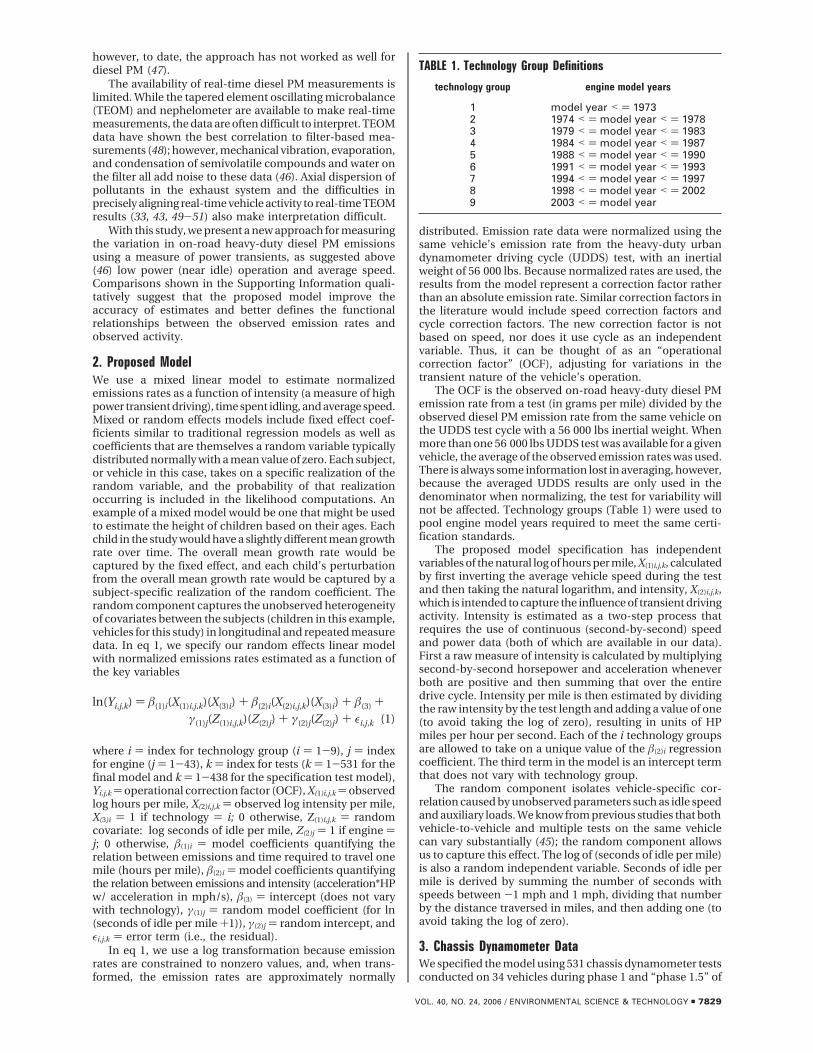
TABLE 1. Technology Group Definitions

technology group engine model years

1 model year < ) 19732 1974 < ) model year < ) 19783 1979 < ) model year < ) 19834 1984 < ) model year < ) 19875 1988 < ) model year < ) 19906 1991 < ) model year < ) 19937 1994 < ) model year < ) 19978 1998 < ) model year < ) 20029 2003 < ) model year

VOL. 40, NO. 24, 2006 / ENVIRONMENTAL SCIENCE & TECHNOLOGY 9 7829

the Coordinating Research Council E55/E59 study (62-64).All of the test vehicles were heavy heavy-duty trucks/truck-tractors; the earliest engine model year was 1973, and thenewest engine model year was 2003. Six of 34 vehicles hadrepairs made to them, and the pre- and postrepair tests weretreated as tests on different vehicles (i.e., the 34 vehicles +repairs are treated as 43 unique vehicles).

The E55/E59 study contained continuous (second-by-second) speed and power data from 8 different test proce-dures; we used the results from the following six cycles: (1)EPA’s schedule D (UDDS); (2) the Australian AC5080; (3)CARB transient; (4) CARB cruise cycles; (5) the HHDDT-Scycle (a shortened version of the CARB high-speed cruisecycle), and (6) the creep34 cycle (four creep3 cycles back-to-back separated by a sharp acceleration to about 8 mph).The results from individual creep3 tests and the idle tests arenot used. We draw a distinction between idle tests, whichcontain only idle, and periods of idle that occur inside atransient cycle; periods of idle embedded within otherwisetransient tests are used in our modeling. The dynamometercycles and a detailed vehicle-dynamometer test matrix isprovided in the Supporting Information.

Table 2 provides the average speed, idle time, intensity,and OCF (normalized diesel PM) for each cycle. The creep34cycle has a lower mean speed and contains more secondsof idle per mile, and its normalized on-road heavy-duty dieselPM emission rates are higher than the other test cycles. Incontrast, the HHDDT-S cycle has the highest mean speedand almost no idle activity and is among the lowestnormalized on-road heavy-duty diesel PM emission rates.These two cycles in effect bound the characteristics of thetruck activity and emissions contained in the data set.

4. ResultsTo fit the model, we divided the 531 chassis dynamometertests from the CRC E55/E59 data into two data subsets. Thefirst subset contained data from 438 tests conducted on thecruise3, trans3, AC5080, and UDDS chassis dynamometerdriving cycles, and the second subset contained 93 testsperformed using the creep34 and HHDDT-S chassis dyna-mometer driving cycles. We specified the model using thefirst subset of data, testing the model using the second subsetof data. In order to identify any serious specification errors,we specified the model using relatively moderate cycles andthen evaluated the model’s suitability when extrapolating tomore extreme cycles. Once our model specification was

considered acceptable, we re-estimated the model using thefull data set, which increases the precision of the estimatedcoefficients. In this section we begin by presenting someinteresting findings from the specification analysis. We thenconclude with a presentation of the final model, which wasspecified using the full data.

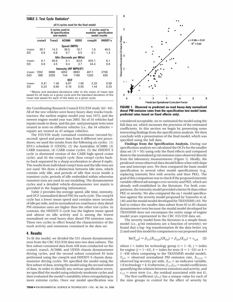
Findings from the Specification Analysis. During ourspecification analysis we calculated the OCFs for the smallerdata set (N ) 93) using only the fixed effects and comparedthem to the normalized g/mi emission rates observed directlyfrom the laboratory measurements (Figure 1). Ideally, thepredicted versus observed data should follow a line with slopeone and intercept zero. We then compared the basic modelspecification to several other model specifications (e.g.,replacing intensity first with severity and then PKE). Thegoal of this comparison was to check if the proposed intensityvariable offered advantages over severity and PKE, which arealready well-established in the literature. For both com-parisons, the intensity model provided a better fit than eitherPKE or severity. We also compared the eq 1 model specifica-tion against the severity model proposed by Yanowitz et al.(46) and the modal model developed for TRANSIMS (44). Wehad to reduce the smaller data subset from 93 to 85 chassisdynamometer tests because the modal model developed forTRANSIMS does not encompass the entire range of enginemodel years represented in the CRC E55/E59 data set.

The severity model from the literature is a simple linearmodel (i.e., g/mi emissions are a function of severity); wefound that a log-log transformation fit the data better (eq2) and used this model for comparison to our proposed model

where i ) index for technology group (i ) 1-9), j ) indexfor engine (j ) 1-43), k ) index for tests (k ) 1-531 or k )1-438 when comparing to the TRANSIMS modal model),Yi,j,k ) observed normalized PM emission rate, X(1)i,j,k )observed log severity per mile, X(2)i ) an indicator variable,1 if technology ) k, 0 otherwise, â(1)i â(2)i ) model coefficientsquantifying the relation between emissions and activity, andεi,j,k ) error term (i.e., the residual associated with test k).

The first coefficient (â(1)i) has a unique value for each ofthe nine groups to control for the effect of severity by

TABLE 2. Test Cycle Statisticsa

all 6 cycles used for the final model

4 cycles used tofit specification

test models

2 cycles used toexamine specification

model results

cruise3 Trans3 AC5080 UDDS creep34 HHDDT-s

Speed (MPH)mean 39.7 14.3 36.5 18.7 1.8 49.0SD 0.6 0.6 0.7 0.5 0.1 1.4

Idle (Seconds per Mile)mean 9.1 50.9 5.1 63.6 925.1 6.1SD 0.6 4.5 0.4 3.7 44.4 0.8

Intensity (HP MPH/S2)mean 1352 8868 4052 6893 4011 2700StD 398 2255 744 1168 1220 635

OCFmean 0.41 1.45 0.67 1.00 2.32 0.59SD 0.23 0.65 0.16 0.05 1.44 0.33

a Means and standard deviations refer to the mean of mean testspeed for all tests on a given cycle and the standard deviation of themean test speed for each of the tests on a given cycle.

FIGURE 1. Observed vs predicted on-road heavy-duty normalizeddiesel PM emission rates from the specification test model (note:predicted rates based on fixed effects only).

ln(Yi,j,k) ) â(1)i(X(1)i,j,k)(X(2)i) + â(2)i(X(2)i) + εi,j,k (2)

7830 9 ENVIRONMENTAL SCIENCE & TECHNOLOGY / VOL. 40, NO. 24, 2006

technology. The second coefficient (â(2)i) provides technologygroup specific values for the intercept. The speed accelerationbins along with their associated gram per second emissionfactors for the modal model are listed in the literature (seeref 44).

Our results suggest that the intensity model provides betteremission estimates than either alternative, with the TRAN-SIMS modal model tending to predict emissions that are toohigh and the severity model tending to predict emissionsthat are too low (see the figure provided in the SupportingInformation).

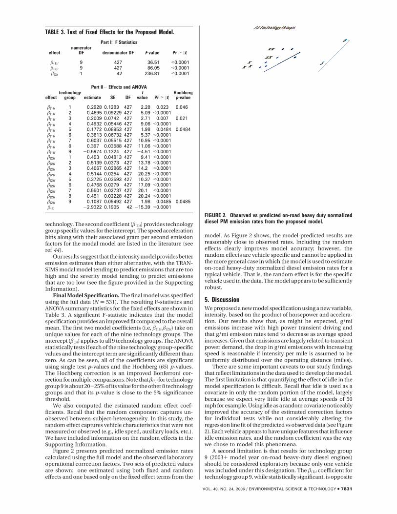
Final Model Specification. The final model was specifiedusing the full data (N ) 531). The resulting F-statistics andANOVA summary statistics for the fixed effects are shown inTable 3. A significant F-statistic indicates that the modelspecification provides an improved fit compared to the overallmean. The first two model coefficients (i.e, â(1)i,â(2)i) take onunique values for each of the nine technology groups. Theintercept (â(3)) applies to all 9 technology groups. The ANOVAstatistically tests if each of the nine technology group-specificvalues and the intercept term are significantly different thanzero. As can be seen, all of the coefficients are significantusing single test p-values and the Hochberg (65) p-values.The Hochberg correction is an improved Bonferroni cor-rection for multiple comparisons. Note that â(2)i for technologygroup 9 is about 20-25% of its value for the other 8 technologygroups and that its p-value is close to the 5% significancethreshold.

We also computed the estimated random effect coef-ficients. Recall that the random component captures un-observed between-subject-heterogeneity. In this study, therandom effect captures vehicle characteristics that were notmeasured or observed (e.g., idle speed, auxiliary loads, etc.).We have included information on the random effects in theSupporting Information.

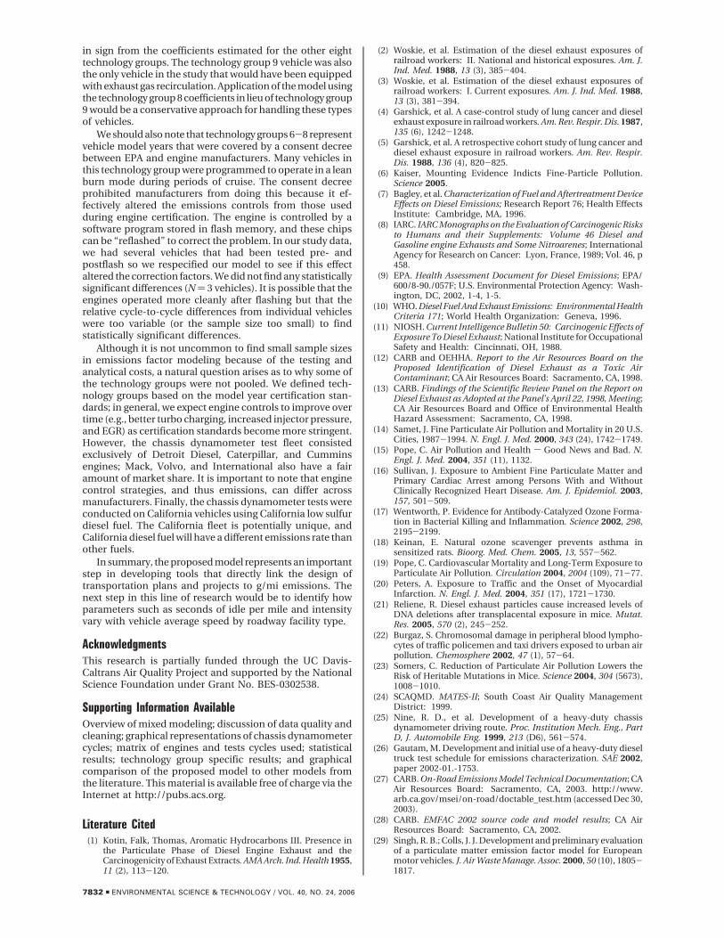
Figure 2 presents predicted normalized emission ratescalculated using the full model and the observed laboratoryoperational correction factors. Two sets of predicted valuesare shown: one estimated using both fixed and randomeffects and one based only on the fixed effect terms from the

model. As Figure 2 shows, the model-predicted results arereasonably close to observed rates. Including the randomeffects clearly improves model accuracy; however, therandom effects are vehicle specific and cannot be applied inthe more general case in which the model is used to estimateon-road heavy-duty normalized diesel emission rates for atypical vehicle. That is, the random effect is for the specificvehicle used in the data. The model appears to be sufficientlyrobust.

5. DiscussionWe proposed a new model specification using a new variable,intensity, based on the product of horsepower and accelera-tion. Our results show that, as might be expected, g/miemissions increase with high power transient driving andthat g/mi emission rates tend to decrease as average speedincreases. Given that emissions are largely related to transientpower demand, the drop in g/mi emissions with increasingspeed is reasonable if intensity per mile is assumed to beuniformly distributed over the operating distance (miles).

There are some important caveats to our study findingsthat reflect limitations in the data used to develop the model.The first limitation is that quantifying the effect of idle in themodel specification is difficult. Recall that idle is used as acovariate in only the random portion of the model, largelybecause we expect very little idle at average speeds of 50mph for example. Using idle as a random covariate noticeablyimproved the accuracy of the estimated correction factorsfor individual tests while not considerably altering theregression line fit of the predicted vs observed data (see Figure2). Each vehicle appears to have unique features that influenceidle emission rates, and the random coefficient was the waywe chose to model this phenomena.

A second limitation is that results for technology group9 (2003+ model year on-road heavy-duty diesel engines)should be considered exploratory because only one vehiclewas included under this designation. The â(1)i coefficient fortechnology group 9, while statistically significant, is opposite

TABLE 3. Test of Fixed Effects for the Proposed Model.

Part I: F Statistics

effectnumerator

DF denominator DF F value Pr > |t|â(1)i 9 427 36.51 <0.0001â(2)i 9 427 86.05 <0.0001â(3) 1 42 236.81 <0.0001

Part II- Effects and ANOVA

effecttechnology

group estimate SE DFt

value Pr > |t|Hochberg

p-value

â(1)i 1 0.2928 0.1283 427 2.28 0.023 0.046â(1)i 2 0.4695 0.09229 427 5.09 <0.0001â(1)i 3 0.2009 0.0742 427 2.71 0.007 0.021â(1)i 4 0.4932 0.05446 427 9.06 <0.0001â(1)i 5 0.1772 0.08953 427 1.98 0.0484 0.0484â(1)i 6 0.3613 0.06732 427 5.37 <0.0001â(1)i 7 0.6037 0.05515 427 10.95 <0.0001â(1)i 8 0.397 0.03588 427 11.06 <0.0001â(1)i 9 -0.5974 0.1324 427 -4.51 <0.0001â(2)i 1 0.453 0.04813 427 9.41 <0.0001â(2)i 2 0.5139 0.0373 427 13.78 <0.0001â(2)i 3 0.4067 0.02865 427 14.2 <0.0001â(2)i 4 0.5144 0.0254 427 20.25 <0.0001â(2)i 5 0.3725 0.03593 427 10.37 <0.0001â(2)i 6 0.4768 0.0279 427 17.09 <0.0001â(2)i 7 0.5501 0.02737 427 20.1 <0.0001â(2)i 8 0.451 0.02228 427 20.24 <0.0001â(2)i 9 0.1087 0.05492 427 1.98 0.0485 0.0485â(3) -2.9322 0.1905 42 -15.39 <0.0001

FIGURE 2. Observed vs predicted on-road heavy duty normalizeddiesel PM emission rates from the proposed model.

VOL. 40, NO. 24, 2006 / ENVIRONMENTAL SCIENCE & TECHNOLOGY 9 7831

in sign from the coefficients estimated for the other eighttechnology groups. The technology group 9 vehicle was alsothe only vehicle in the study that would have been equippedwith exhaust gas recirculation. Application of the model usingthe technology group 8 coefficients in lieu of technology group9 would be a conservative approach for handling these typesof vehicles.

We should also note that technology groups 6-8 representvehicle model years that were covered by a consent decreebetween EPA and engine manufacturers. Many vehicles inthis technology group were programmed to operate in a leanburn mode during periods of cruise. The consent decreeprohibited manufacturers from doing this because it ef-fectively altered the emissions controls from those usedduring engine certification. The engine is controlled by asoftware program stored in flash memory, and these chipscan be “reflashed” to correct the problem. In our study data,we had several vehicles that had been tested pre- andpostflash so we respecified our model to see if this effectaltered the correction factors. We did not find any statisticallysignificant differences (N ) 3 vehicles). It is possible that theengines operated more cleanly after flashing but that therelative cycle-to-cycle differences from individual vehicleswere too variable (or the sample size too small) to findstatistically significant differences.

Although it is not uncommon to find small sample sizesin emissions factor modeling because of the testing andanalytical costs, a natural question arises as to why some ofthe technology groups were not pooled. We defined tech-nology groups based on the model year certification stan-dards; in general, we expect engine controls to improve overtime (e.g., better turbo charging, increased injector pressure,and EGR) as certification standards become more stringent.However, the chassis dynamometer test fleet consistedexclusively of Detroit Diesel, Caterpillar, and Cumminsengines; Mack, Volvo, and International also have a fairamount of market share. It is important to note that enginecontrol strategies, and thus emissions, can differ acrossmanufacturers. Finally, the chassis dynamometer tests wereconducted on California vehicles using California low sulfurdiesel fuel. The California fleet is potentially unique, andCalifornia diesel fuel will have a different emissions rate thanother fuels.

In summary, the proposed model represents an importantstep in developing tools that directly link the design oftransportation plans and projects to g/mi emissions. Thenext step in this line of research would be to identify howparameters such as seconds of idle per mile and intensityvary with vehicle average speed by roadway facility type.

AcknowledgmentsThis research is partially funded through the UC Davis-Caltrans Air Quality Project and supported by the NationalScience Foundation under Grant No. BES-0302538.

Supporting Information AvailableOverview of mixed modeling; discussion of data quality andcleaning; graphical representations of chassis dynamometercycles; matrix of engines and tests cycles used; statisticalresults; technology group specific results; and graphicalcomparison of the proposed model to other models fromthe literature. This material is available free of charge via theInternet at http://pubs.acs.org.

Literature Cited(1) Kotin, Falk, Thomas, Aromatic Hydrocarbons III. Presence in

the Particulate Phase of Diesel Engine Exhaust and theCarcinogenicity of Exhaust Extracts. AMA Arch. Ind. Health 1955,11 (2), 113-120.

(2) Woskie, et al. Estimation of the diesel exhaust exposures ofrailroad workers: II. National and historical exposures. Am. J.Ind. Med. 1988, 13 (3), 385-404.

(3) Woskie, et al. Estimation of the diesel exhaust exposures ofrailroad workers: I. Current exposures. Am. J. Ind. Med. 1988,13 (3), 381-394.

(4) Garshick, et al. A case-control study of lung cancer and dieselexhaust exposure in railroad workers. Am. Rev. Respir. Dis. 1987,135 (6), 1242-1248.

(5) Garshick, et al. A retrospective cohort study of lung cancer anddiesel exhaust exposure in railroad workers. Am. Rev. Respir.Dis. 1988, 136 (4), 820-825.

(6) Kaiser, Mounting Evidence Indicts Fine-Particle Pollution.Science 2005.

(7) Bagley, et al. Characterization of Fuel and Aftertreatment DeviceEffects on Diesel Emissions; Research Report 76; Health EffectsInstitute: Cambridge, MA, 1996.

(8) IARC. IARC Monographs on the Evaluation of Carcinogenic Risksto Humans and their Supplements: Volume 46 Diesel andGasoline engine Exhausts and Some Nitroarenes; InternationalAgency for Research on Cancer: Lyon, France, 1989; Vol. 46, p458.

(9) EPA. Health Assessment Document for Diesel Emissions; EPA/600/8-90./057F; U.S. Environmental Protection Agency: Wash-ington, DC, 2002, 1-4, 1-5.

(10) WHO. Diesel Fuel And Exhaust Emissions: Environmental HealthCriteria 171; World Health Organization: Geneva, 1996.

(11) NIOSH. Current Intelligence Bulletin 50: Carcinogenic Effects ofExposure To Diesel Exhaust; National Institute for OccupationalSafety and Health: Cincinnati, OH, 1988.

(12) CARB and OEHHA. Report to the Air Resources Board on theProposed Identification of Diesel Exhaust as a Toxic AirContaminant; CA Air Resources Board: Sacramento, CA, 1998.

(13) CARB. Findings of the Scientific Review Panel on the Report onDiesel Exhaust as Adopted at the Panel’s April 22, 1998, Meeting;CA Air Resources Board and Office of Environmental HealthHazard Assessment: Sacramento, CA, 1998.

(14) Samet, J. Fine Particulate Air Pollution and Mortality in 20 U.S.Cities, 1987-1994. N. Engl. J. Med. 2000, 343 (24), 1742-1749.

(15) Pope, C. Air Pollution and Health s Good News and Bad. N.Engl. J. Med. 2004, 351 (11), 1132.

(16) Sullivan, J. Exposure to Ambient Fine Particulate Matter andPrimary Cardiac Arrest among Persons With and WithoutClinically Recognized Heart Disease. Am. J. Epidemiol. 2003,157, 501-509.

(17) Wentworth, P. Evidence for Antibody-Catalyzed Ozone Forma-tion in Bacterial Killing and Inflammation. Science 2002, 298,2195-2199.

(18) Keinan, E. Natural ozone scavenger prevents asthma insensitized rats. Bioorg. Med. Chem. 2005, 13, 557-562.

(19) Pope, C. Cardiovascular Mortality and Long-Term Exposure toParticulate Air Pollution. Circulation 2004, 2004 (109), 71-77.

(20) Peters, A. Exposure to Traffic and the Onset of MyocardialInfarction. N. Engl. J. Med. 2004, 351 (17), 1721-1730.

(21) Reliene, R. Diesel exhaust particles cause increased levels ofDNA deletions after transplacental exposure in mice. Mutat.Res. 2005, 570 (2), 245-252.

(22) Burgaz, S. Chromosomal damage in peripheral blood lympho-cytes of traffic policemen and taxi drivers exposed to urban airpollution. Chemosphere 2002, 47 (1), 57-64.

(23) Somers, C. Reduction of Particulate Air Pollution Lowers theRisk of Heritable Mutations in Mice. Science 2004, 304 (5673),1008-1010.

(24) SCAQMD. MATES-II; South Coast Air Quality ManagementDistrict: 1999.

(25) Nine, R. D., et al. Development of a heavy-duty chassisdynamometer driving route. Proc. Institution Mech. Eng., PartD, J. Automobile Eng. 1999, 213 (D6), 561-574.

(26) Gautam, M. Development and initial use of a heavy-duty dieseltruck test schedule for emissions characterization. SAE 2002,paper 2002-01.-1753.

(27) CARB. On-Road Emissions Model Technical Documentation; CAAir Resources Board: Sacramento, CA, 2003. http://www.arb.ca.gov/msei/on-road/doctable_test.htm (accessed Dec 30,2003).

(28) CARB. EMFAC 2002 source code and model results; CA AirResources Board: Sacramento, CA, 2002.

(29) Singh, R. B.; Colls, J. J. Development and preliminary evaluationof a particulate matter emission factor model for Europeanmotor vehicles. J. Air Waste Manage. Assoc. 2000, 50 (10), 1805-1817.

7832 9 ENVIRONMENTAL SCIENCE & TECHNOLOGY / VOL. 40, NO. 24, 2006

(30) Singh, R. B.; Colls, J. J. Development of Particulate EmissionFactors and Size Distributions for European Motor Vehicles(97-WP96.01). In AWMA 90th Annual Meeting & Exhibition, June8-13, 1997; Air & Waste Management Association: Toronto,Ontario, Canada, 1997.

(31) Singh, R. B.; Colls, J. J. Development of a Particulate EmissionFactor Model for European Motor Vehicles (97-RP143.01). InAWMA 90th Annual Meeting & Exhibition, June 8-13, 1997, Air& Waste Management Association: Toronto, Ontario, Canada,1997.

(32) Singh, R.; Huber, A.; Braddock, J. Development of a MicroscaleEmission Factor Model for Particulate Matter for PredictingReal-Time Motor Vehicle Emissions. J. Air Waste Manage. Assoc.2003, 53 (10), 1204-1217.

(33) Clark, N. Translation of distance-specific emissions ratesbetween different heavy-duty vehicle chassis test schedules.SAE 2002, paper 2002-01.-1754.

(34) Niemeier, D. A. Spatial Applicability of Emission Factors forModeling Mobile Emissions. Environ. Sci. Technol. 2002, 36 (4),736-741.

(35) Browning, L. Update Heavy-Duty Engine Emission ConversionFactors for MOBILE6: Analysis of BSFCs and Calculation ofHeavy-Duty Engine Emission Conversion Factors; EPA: 1998.

(36) Browning, L. Update Heavy-Duty Engine Emission Conver-sion Factors for MOBILE6: Analysis of Fuel Economy, Non-Engine Fuel Economy Improvements and Fuel Densities; EPA:1998.

(37) Machiele, P. Heavy-duty Vehicle Emission Conversion Factors II(1962-2000); EPA-AA-SDSB-89-01; United States EnvironmentalProtection Agency: 1988.

(38) Glover, E. Cumberworth, MOBILE6.1 Particulate Emission FactorModel Technical Description Printed on Recycled Paper (FinalReport); EPA420-R-03-001; United States Environmental Pro-tection Agency: 2003.

(39) EPA. DRAFT Users Guide to Part5: A Program for CalculatingParticle Emissions from Motor Vehicles; EPA-AA-AQAB-94-2;United States Environmental Protection Agency, Office of Airand Radiation: 1995.

(40) Jarrett, R.; Clark, N. Evaluation of methods for determiningcontinuous particulate matter from transient testing of heavy-duty diesel engines. SAE 2001, paper 2001-01.-3575.

(41) Hofeldt, D.; Chen, G. Transient particulate emissions from dieselbuses during the central business district cycle. SAE 1996, paper960251.

(42) Clark, N. N.; Jarrett, R. P.; Atkinson, C. M. Field measurementsof particulate matter emissions, carbon monoxide, and exhaustopacity from heavy-duty diesel vehicles. J. Air Waste Manage.Assoc. 1999, 49 (Special Issue SI), 76-84.

(43) Ramamurthy, R. Models for predicting transient heavy-dutyvehicle emissions. SAE 1998, technical paper 982652.

(44) Clark, N. N.; Gajendran, P.; Kern, J. M. A Predictive Tool forEmissions from Heavy-Duty Diesel Vehicles. Environ. Sci. Technol.2003, 37 (1), 7-15.

(45) Clark, N. Diesel and CNG transit bus emissions characterizationby two chassis dynamometer laboratories: Results and issues.SAE 1999, paper 1999-01.-1469.

(46) Yanowitz, J.; Graboski, M.; McCormick, R. Prediction of In-UseEmissions of Heavy-Duty Diesel Vehicles from Engine Testing.Environ. Sci. Technol. 2002, 36 (2), 270-275.

(47) Taylor, S. Diesel emissions prediction from dissimilar cyclescaling. Proc. Institution Mech. Eng. Part D, J. Automobile Eng.2004, 218 (3).

(48) Moosmuller, H. Time-Resolved Characterization of DieselParticulate Emissions. 1. Instruments for Particle Mass Mea-surements. Environ. Sci. Technol. 2001, 35 (4), 781 -787.

(49) Ramamurthy, R.; Clark, N. N. Atmospheric Emissions InventoryData for Heavy-Duty Vehicles. Environ. Sci. Technol. 1999, 33(1), 55 -62.

(50) Messer, T.; Clark, N.; Lyons, D. Measurement delays and modalanalysis for a heavy duty transportable emissions testinglaboratory. SAE 1995, paper 950218.

(51) Ganesan, B.; Clark, N. Relationships between instantaneousand measured emissions in heavy-duty applications. SAE 2001,paper 2001-01.-33536.

(52) Zhang, K.; Wexler, A. Evolution of particle number distributionnear roadwayssPart I: analysis of aerosol dynamics and itsimplications for engine emission measurement. Atmos. Environ.2004, 38 (38), 6643-6653.

(53) Palmgren, F. Actual car fleet emissions estimated from urbanair quality measurements and street pollution models. Sci. TotalEnviron. 1999, 235 (1-3), 101-109.

(54) Hall, D. Measurement of the number and size distribution ofparticle emissions from heavy-duty engines. SAE 2000, paper2000-01.-2000.

(55) Hlavinka, M.; Bullin, J. Validation of Mobile Source EmissionEstimates using Mass Balance Techniques. J. Air Pollut. ControlAssoc. 1988, 38 (8), 1035-1039.

(56) Bullin, J.; Green, Polasek, et al. Determination of vehicle emis-sion rates from roadways by mass balance techniques. Environ.Sci. Technol. 1980, 14 (6), 700-705.

(57) Ketzel, M. Particle and trace gas emission factors underurban driving conditions in Copenhagen based on streetand roof-level observations. Atmos. Environ. 2003, 37, 2735-2749.

(58) Shah, S. Emission Rates of Particulate Matter and Elementaland Organic Carbon from In-Use Diesel Engines. Environ. Sci.Technol. 2004, 38 (9), 2544-2550.

(59) Shah, S. Emission rates of regulated pollutants from on-roadheavy-duty diesel vehicles. Atmos. Environ. 2005, 40 (1), 147-153.

(60) Cocker, D. Development and Application of a Mobile Laboratoryfor Measuring Emissions from Diesel Engines. 2. Sampling forToxics and Particulate Matter. Environ. Sci. Technol. 2004, 38(24), 6809-6816.

(61) Cocker, D. Development and Application of a Mobile Laboratoryfor Measuring Emissions from Diesel Engines. 1. Regulatedgaseous Emissions. Environ. Sci. Technol. 2004, 38 (7), 2182-2189.

(62) CRC. Heavy-Heavy Vehicle Chassis Dynamometer Testing ForEmissions Inventory, Air Quality Modeling, Source Apportion-ment and Air Toxics Emission Inventory: CRC Project E55/E59Phase I Interim Report; CRC: Alpharetta, GA, 2002.

(63) CRC. California Heavy-Heavy Duty Truck Emissions Charac-terization for Project E55/E59-1.5; Draft Final Report; CRC:Alpharetta, GA, 2003.

(64) CARB. CRC E55/E59 Data sets, Phase 1 & phase 1.5; 2004;Sacramento, CA.

(65) Hochberg, A Sharper Bonferroni Procedure for Multiple Sig-nificance Testing. Biometrika 1988, 75, 800-803.

Received for review January 25, 2006. Revised manuscriptreceived July 27, 2006. Accepted October 2, 2006.

ES060177E

VOL. 40, NO. 24, 2006 / ENVIRONMENTAL SCIENCE & TECHNOLOGY 9 7833