On Periodicity Detection and Structural Periodic Similarity

Michail Vlachos Philip Yu Vittorio Castelli

IBM T.J. Watson Research Center19 Skyline Dr, Hawthorne, NY

Abstract

This work motivates the need for more flexible structural

similarity measures between time-series sequences, which

are based on the extraction of important periodic features.

Specifically, we present non-parametric methods for accurate

periodicity detection and we introduce new periodic distance

measures for time-series sequences. The goal of these tools

and techniques are to assist in detecting, monitoring and

visualizing structural periodic changes. It is our belief that

these methods can be directly applicable in the manufacturing

industry for preventive maintenance and in the medical sci-

ences for accurate classification and anomaly detection.

1 Introduction

In spite of the fact that in the past decade we haveexperienced a profusion of time-series distance measuresand representations [9], the majority of them attemptto characterize the similarity between sequences basedsolely on shape. However, it is becoming increasinglyapparent that structural similarities can provide moreintuitive sequence characterizations that adhere moretightly to human perception of similarity.

While shape-based similarity methods seek to iden-tify homomorphic sequences using the original raw data,structure-based methodologies are designed to find la-tent similarities, possibly by transforming the sequencesinto a new domain, where the resemblance can be moreapparent. For example, in [6] the authors use change-point-detection signatures for identifying sequences thatexhibit similar structural changes. In [7] Kalpakis, etal., use the cepstrum for clustering sequences that sharea similar underlying ARIMA generative process. Keogh,et al. [10], employ a compression-based dissimilaritymeasure that is effectively used for clustering and anom-aly detection. Finally, Vlachos, et al. [15] considerstructural similarities that are based on burst featuresof time-series sequences.

In this work we consider methods for efficiently cap-turing and characterizing the periodicity and periodicsimilarity of time-series. Such techniques can be ap-plicable in a variety of disciplines, such as manufactur-ing, natural sciences and medicine, which acquire and

record large amounts of periodic data. For the analysisof such data, first there is a need for accurate periodic-ity estimation, which can be utilized either for anomalydetection or for prediction purposes. Then, a structuraldistance measure should be deployed that can effectivelyincorporate the periodicity for quantifying the degree ofsimilarity between sequences. A periodic measure canallow for more meaningful and accurate clustering andclassification, and can also be used for interactive explo-ration (and visualization) of massive periodic datasets.Let us consider areas where periodic measures can beapplicable:

In natural sciences, many processes manifeststrong or weak periodic behavior, such as tidal pat-terns (oceanography), sunspots (astronomy), tempera-ture changes (meteorology), etc. Periodic analysis andperiodicity estimation is an important aspect in thesedisciplines, because they can suggest potential anom-alies or help understand the causal relationship betweendifferent processes. For example, it is well establishedthat solar variability greatly affects the climate change.In fact the solar cycle (sunspot numbers) presents strik-ing resemblance to the northern hemisphere land tem-peratures [4].

In medicine, where many biometric measures(e.g., heartbeats) exhibit strong periodicities, thereis a great interest in detecting periodic anomalies.Disturbances of similar periodic patterns can be notedin many degenerative diseases; for example, it hasbeen noted that Tourette’s syndrome patients exhibitelevated eyeblink rate [14], while people affected byParkison’s disease show symptoms of gait disturbances[1]. The tools that we provide here, can significantlyenhance the early detection of such changes.

Finally, periodic analysis is an indispensable toolin automotive, aviation and manufacturing industriesfor machine monitoring and diagnostics [12]. Predic-tive maintenance can be possible by examination of thevibration spectrum caused by its rotating parts. There-fore, a change in the periodic structure of machine vi-brations can be a good indicator of machine wear and/orof an incipient failure.

This work targets similar applications and providestools that can significantly ease the “mining” of usefulinformation. Specifically, this paper makes the followingcontributions:

1. We present a novel automatic method for accurateperiodicity detection in time-series data. Our algorithmis the first one that exploits the information in bothperiodogram and autocorrelation to provide accurateperiodic estimates without upsampling.

2. We introduce new periodic distance measures thatexploit the power of the dominant periods, as providedby the Fourier Transform. By ignoring the phase infor-mation we can provide more compact representations,that also capture similarities under time-shift transfor-mations.

3. Finally, we present comprehensive experimentsdemonstrating the applicability and efficiency of theproposed methods, on a variety of real world datasets(online query logs, manufacturing diagnostics, medicaldata, etc.).

2 Background

We provide a brief introduction to harmonic analysisusing the discrete Fourier Transform, because we willuse these tools as the building blocks of our algorithms.

2.1 Discrete Fourier Transform. The normalizedDiscrete Fourier Transform of a sequence x(n), n =0, 1 . . . N − 1 is a sequence of complex numbers X(f):

X(fk/N ) = 1√N

N−1�

n=0

x(n)e−j2πkn

N , k = 0, 1 . . . N − 1

where the subscript k/N denotes the frequency thateach coefficient captures. Throughout the text we willalso utilize the notation F(x) to describe the FourierTransform. Since we are dealing with real signals, theFourier coefficients are symmetric around the middleone (or to be more exact, they will be the complexconjugate of their symmetric). The Fourier transformrepresents the original signal as a linear combination of

the complex sinusoids sf (n) = ej2πfn/N√

N. Therefore, the

Fourier coefficients record the amplitude and phase ofthese sinusoids, after signal x is projected on them.

We can return from the frequency domain back tothe time domain, using the inverse Fourier transformF−1(x) ≡ x(n):

x(n) = 1√N

N−1�

k=0

X(fk/N )ej2πkn

N , n = 0, 1 . . . N − 1

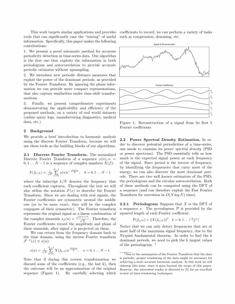
Note that if during this reverse transformation wediscard some of the coefficients (e.g., the last k), thenthe outcome will be an approximation of the originalsequence (Figure 1). By carefully selecting which

coefficients to record, we can perform a variety of taskssuch as compression, denoising, etc.

Signal & Reconstruction

f1

Fourier Coefficients

f2

f3

f4

f0

Figure 1: Reconstruction of a signal from its first 5Fourier coefficients

2.2 Power Spectral Density Estimation. In or-der to discover potential periodicities of a time-series,one needs to examine its power spectral density (PSDor power spectrum). The PSD essentially tells us howmuch is the expected signal power at each frequencyof the signal. Since period is the inverse of frequency,by identifying the frequencies that carry most of theenergy, we can also discover the most dominant peri-ods. There are two well known estimators of the PSD;the periodogram and the circular autocorrelation. Bothof these methods can be computed using the DFT ofa sequence (and can therefore exploit the Fast FourierTransform for execution in O(N log N) time).

2.2.1 Periodogram Suppose that X is the DFT ofa sequence x. The periodogram P is provided by thesquared length of each Fourier coefficient:

P(fk/N ) = ‖X(fk/N )‖2 k = 0, 1 . . . dN−1

2e

Notice that we can only detect frequencies that are atmost half of the maximum signal frequency, due to theNyquist fundamental theorem. In order to find the kdominant periods, we need to pick the k largest valuesof the periodogram. 1

1Due to the assumption of the Fourier Transform that the data

is periodic, proper windowing of the data might be necessary forachieving a more accurate harmonic analysis. In this work we will

sidestep this issue, since it goes beyond the scope of this paper.

However, the interested reader is directed to [5] for an excellent

review of data windowing techniques.

Each element of the periodogram provides thepower at frequency k/N or, equivalently, at period N/k.Being more precise, each DFT ‘bin’ corresponds to arange of periods (or frequencies). That is, coefficientX(fk/N ) corresponds to periods [N

k . . . Nk−1 ). It is easy

to see that the resolution of the periodogram becomesvery coarse for longer periods. For example, for a se-quence of length N = 256, the DFT bin margins will beN/1, N/2, N/3, . . . = 256, 128, 64 etc.

Essentially, the accuracy of the discovered periods,deteriorates for large periods, due to the increasingwidth of the DFT bins (N/k). Another related issue isspectral leakage, which causes frequencies that are notinteger multiples of the DFT bin width, to disperse overthe entire spectrum. This can lead to ‘false alarms’in the periodogram. However, the periodogram canstill provide an accurate indicator of important short(to medium) length periods. Additionally, through theperiodogram it is easy to automate the extraction ofimportant periods (peaks) by examining the statisticalproperties of the Fourier coefficients (such as in [15]).

2.2.2 Circular Autocorrelation. The second wayto estimate the dominant periods of a time-series x, isto calculate the circular AutoCorrelation Function (orACF), which examines how similar a sequence is to itsprevious values for different τ lags:

ACF (τ) = 1

N

N−1�

n=0

x(τ) · x(n + τ)

Therefore, the autocorrelation is formally a convo-lution, and we can avoid the quadratic calculation inthe time domain by computing it efficiently as a dotproduct in the frequency domain using the normalizedFourier transform:

ACF = F−1 < X, X∗ >

The star (∗) symbol denotes complex conjugation.The ACF provides a more fine-grained periodicity

detector than the periodogram, hence it can pinpointwith greater accuracy even larger periods. However,it is not sufficient by itself for automatic periodicitydiscovery for the following reasons:

1. Automated discovery of important peaks ismore difficult than in the periodogram. Approachesthat utilize forms of autocorrelation require the userto manually set the significance threshold (such as in[2, 3]).

2. Even if the user picks the level of significance,multiples of the same basic period also appear as peaks.Therefore, the method introduces many false alarmsthat need to be eliminated in a post-processing phase.

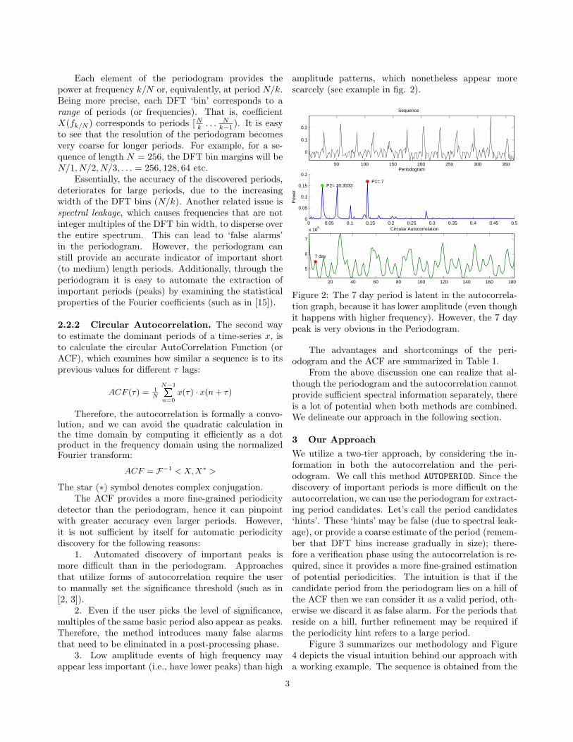
3. Low amplitude events of high frequency mayappear less important (i.e., have lower peaks) than high

amplitude patterns, which nonetheless appear morescarcely (see example in fig. 2).

50 100 150 200 250 300 350

0

0.1

0.2

Sequence

0 0.05 0.1 0.15 0.2 0.25 0.3 0.35 0.4 0.45 0.50

0.05

0.1

0.15

0.2

Pow

er

Periodogram

P1= 7P2= 30.3333

20 40 60 80 100 120 140 160 180

5

6

7

x 106 Circular Autocorrelation

7 day

Figure 2: The 7 day period is latent in the autocorrela-tion graph, because it has lower amplitude (even thoughit happens with higher frequency). However, the 7 daypeak is very obvious in the Periodogram.

The advantages and shortcomings of the peri-odogram and the ACF are summarized in Table 1.

From the above discussion one can realize that al-though the periodogram and the autocorrelation cannotprovide sufficient spectral information separately, thereis a lot of potential when both methods are combined.We delineate our approach in the following section.

3 Our Approach

We utilize a two-tier approach, by considering the in-formation in both the autocorrelation and the peri-odogram. We call this method AUTOPERIOD. Since thediscovery of important periods is more difficult on theautocorrelation, we can use the periodogram for extract-ing period candidates. Let’s call the period candidates‘hints’. These ‘hints’ may be false (due to spectral leak-age), or provide a coarse estimate of the period (remem-ber that DFT bins increase gradually in size); there-fore a verification phase using the autocorrelation is re-quired, since it provides a more fine-grained estimationof potential periodicities. The intuition is that if thecandidate period from the periodogram lies on a hill ofthe ACF then we can consider it as a valid period, oth-erwise we discard it as false alarm. For the periods thatreside on a hill, further refinement may be required ifthe periodicity hint refers to a large period.

Figure 3 summarizes our methodology and Figure4 depicts the visual intuition behind our approach witha working example. The sequence is obtained from the

3

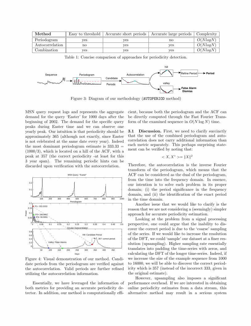
Method Easy to threshold Accurate short periods Accurate large periods Complexity

Periodogram yes yes no O(NlogN)Autocorrelation no yes yes O(NlogN)Combination yes yes yes O(NlogN)

Table 1: Concise comparison of approaches for periodicity detection.

Sequence Autocorrelation

hill

valley

Periodogram Refine Period

Candidate Periods

False Alarm

Dismiss

Period

Figure 3: Diagram of our methodology (AUTOPERIOD method)

MSN query request logs and represents the aggregatedemand for the query ‘Easter’ for 1000 days after thebeginning of 2002. The demand for the specific querypeaks during Easter time and we can observe oneyearly peak. Our intuition is that periodicity should beapproximately 365 (although not exactly, since Easteris not celebrated at the same date every year). Indeedthe most dominant periodogram estimate is 333.33 =(1000/3), which is located on a hill of the ACF, with apeak at 357 (the correct periodicity -at least for this3 year span). The remaining periodic hints can bediscarded upon verification with the autocorrelation.

100 200 300 400 500 600 700 800 900 10000

0.1

0.2

MSN Query: "Easter"

0 0.05 0.1 0.15 0.2 0.25 0.3 0.35 0.4 0.45 0.50

0.05

0.1

0.15

0.2

Pow

er

Periodogram

P1= 333.3333

P2= 166.6667P3= 90.9091

50 100 150 200 250 300 350 400 450

0

0.2

0.4

0.6

0.8

Days

Circular Autocorrelation

Hill: Candidate Period

Valley: False Alarms

357: correct period

Figure 4: Visual demonstration of our method. Candi-date periods from the periodogram are verified againstthe autocorrelation. Valid periods are further refinedutilizing the autocorrelation information.

Essentially, we have leveraged the information ofboth metrics for providing an accurate periodicity de-tector. In addition, our method is computationally effi-

cient, because both the periodogram and the ACF canbe directly computed through the Fast Fourier Trans-form of the examined sequence in O(N log N) time.

3.1 Discussion. First, we need to clarify succinctlythat the use of the combined periodogram and auto-correlation does not carry additional information thaneach metric separately. This perhaps surprising state-ment can be verified by noting that:

< X, X∗ >= ‖X‖2

Therefore, the autocorrelation is the inverse Fouriertransform of the periodogram, which means that theACF can be considered as the dual of the periodogram,from the time into the frequency domain. In essence,our intention is to solve each problem in its properdomain; (i) the period significance in the frequencydomain, and (ii) the identification of the exact periodin the time domain.

Another issue that we would like to clarify is thereason that we are not considering a (seemingly) simplerapproach for accurate periodicity estimation.

Looking at the problem from a signal processingperspective, one could argue that the inability to dis-cover the correct period is due to the ‘coarse’ samplingof the series. If we would like to increase the resolutionof the DFT, we could ‘sample’ our dataset at a finer res-olution (upsampling). Higher sampling rate essentiallytranslates into padding the time-series with zeros, andcalculating the DFT of the longer time-series. Indeed, ifwe increase the size of the example sequence from 1000to 16000, we will be able to discover the correct period-icity which is 357 (instead of the incorrect 333, given inthe original estimate).

However, upsampling also imposes a significantperformance overhead. If we are interested in obtainingonline periodicity estimates from a data stream, thisalternative method may result in a serious system

bottleneck. We can see this analytically; the timerequired to compute the FFT of a sequence with length2x is in the order of 2xlog2x = x2x. Now let’s assumethat we pad the sequence with zeros increasing its length16 times (just like in our working example). The FFTnow requires time in the order of (x + 4)2x+4, whichafter algebraic calculations translates into 2 orders ofmagnitude additional time.

Using our methodology, we do not require highersampling rates for the FFT calculation, hence keepinga low computational profile.

3.2 Discovery of Candidate Periods. For extract-ing a set of candidate periodicities from the peri-odogram, one needs to determine an appropriate powerthreshold that should distinguish only the dominant fre-quencies (or inversely the dominant periods). If none ofthe sequence frequencies exceeds the specific threshold(i.e., the set of periodicity ‘hints’ is empty), then we canregard the sequence as non-periodic.

In order to specify which periods are important, wefirst need to identify how much of the signal energy isattributed to random mechanisms, that is, everythingthat could not have been attributed to a random processshould be of interest.

Let us assume that we examine a sequence x. Theoutcome of a permutation on the elements of x is asequence x. The new sequence will retain the first orderstatistics of the original sequence, but will not exhibitany pattern or periodicities, because of the ’scrambling’process (even though such characteristics may haveexisted in sequence x). Anything that has the structureof x is not interesting and should be discarded, thereforeat this step we can record the maximum power (pmax)that x exhibits, at any frequency f .

pmax = arg maxf

‖X(f)‖2

Only if a frequency of x has more power than pmax canbe considered interesting. If we would like to providea 99% confidence interval on what frequencies areimportant, we should repeat the above experiment 100times and record for each one the maximum power of thepermuted sequence x. The 99th largest value of these100 experiments, will provide a sufficient estimator ofthe power threshold pT that we are seeking. Periods(in the original sequence periodogram) whose power ismore than the derived threshold will be considered:

phint = {N/k : P(fk/N ) > pT }

Finally, an additional period ‘trimming’ should be per-formed for discarding periods that are either too largeor too small and therefore cannot be considered reli-

able. In this phase any periodic hint greater than N/2or smaller than 2 is removed.

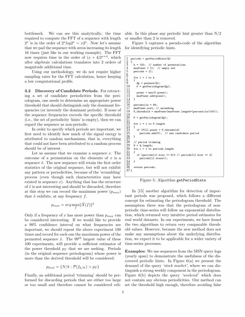
Figure 5 captures a pseudo-code of the algorithmfor identifying periodic hints.

1 periods = getPeriodHints(Q)

2 {3 k = 100; // number of permutations

4 maxPower = {}; // empty set

5 periods = {};

67 for i = 1 to k8 {9 Qp = permute(Q);

10 P = getPeriodogram(Qp);

1112 power = max(P.power);

13 maxPower.add(power);

14 }1516 percentile = 99;

17 maxPower.sort; // ascending

18 P_threshold = maxPower(maxPower.length*(percentile/100));

1920 P = getPeriodogram(Qp);

2122 for i = 1 to P.length

23 {24 if (P[i].power > P_threshold)

25 periods.add(P); // new candidate period

26 }2728 // period trimming

29 N = Q.length;

30 for i = 1 to periods.length

31 {32 if (periods[i].hint >= N/2 || periods[i].hint <= 2)

33 periods[i].erase();

34 }3536 return periods;

37 }

Figure 5: Algorithm getPeriodHints

In [15] another algorithm for detection of impor-tant periods was proposed, which follows a differentconcept for estimating the periodogram threshold. Theassumption there was that the periodogram of non-periodic time-series will follow an exponential distribu-tion, which returned very intuitive period estimates forreal world datasets. In our experiments, we have foundthe two algorithms to return very comparable thresh-old values. However, because the new method does notmake any assumptions about the underlying distribu-tion, we expect it to be applicable for a wider variety oftime-series processes.

Examples: We use sequences from the MSN query logs(yearly span) to demonstrate the usefulness of the dis-covered periodic hints. In Figure 6(a) we present thedemand of the query ‘stock market’, where we can dis-tinguish a strong weekly component in the periodogram.Figure 6(b) depicts the query ‘weekend’ which doesnot contain any obvious periodicities. Our method canset the threshold high enough, therefore avoiding false

5

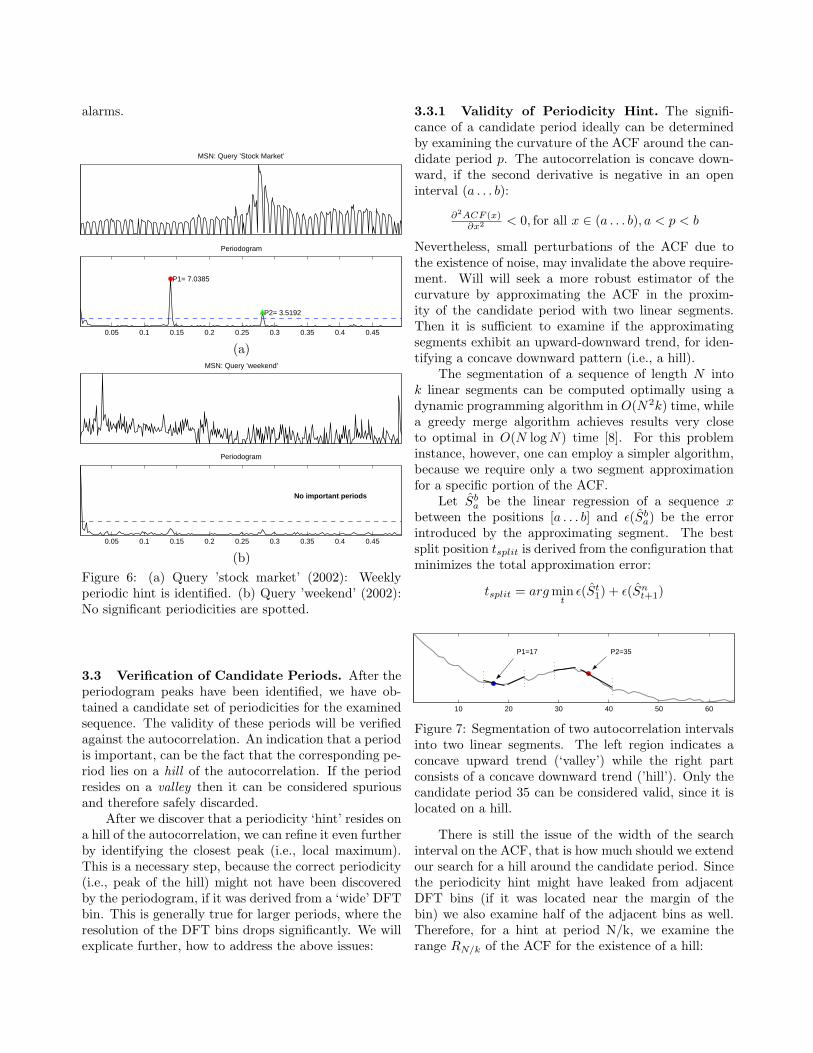
alarms.

MSN: Query ’Stock Market’

0.05 0.1 0.15 0.2 0.25 0.3 0.35 0.4 0.45

Periodogram

P1= 7.0385

P2= 3.5192

(a)MSN: Query ’weekend’

0.05 0.1 0.15 0.2 0.25 0.3 0.35 0.4 0.45

Periodogram

No important periods

(b)

Figure 6: (a) Query ’stock market’ (2002): Weeklyperiodic hint is identified. (b) Query ’weekend’ (2002):No significant periodicities are spotted.

3.3 Verification of Candidate Periods. After theperiodogram peaks have been identified, we have ob-tained a candidate set of periodicities for the examinedsequence. The validity of these periods will be verifiedagainst the autocorrelation. An indication that a periodis important, can be the fact that the corresponding pe-riod lies on a hill of the autocorrelation. If the periodresides on a valley then it can be considered spuriousand therefore safely discarded.

After we discover that a periodicity ‘hint’ resides ona hill of the autocorrelation, we can refine it even furtherby identifying the closest peak (i.e., local maximum).This is a necessary step, because the correct periodicity(i.e., peak of the hill) might not have been discoveredby the periodogram, if it was derived from a ‘wide’ DFTbin. This is generally true for larger periods, where theresolution of the DFT bins drops significantly. We willexplicate further, how to address the above issues:

3.3.1 Validity of Periodicity Hint. The signifi-cance of a candidate period ideally can be determinedby examining the curvature of the ACF around the can-didate period p. The autocorrelation is concave down-ward, if the second derivative is negative in an openinterval (a . . . b):

∂2ACF (x)∂x2 < 0, for all x ∈ (a . . . b), a < p < b

Nevertheless, small perturbations of the ACF due tothe existence of noise, may invalidate the above require-ment. Will will seek a more robust estimator of thecurvature by approximating the ACF in the proxim-ity of the candidate period with two linear segments.Then it is sufficient to examine if the approximatingsegments exhibit an upward-downward trend, for iden-tifying a concave downward pattern (i.e., a hill).

The segmentation of a sequence of length N intok linear segments can be computed optimally using adynamic programming algorithm in O(N2k) time, whilea greedy merge algorithm achieves results very closeto optimal in O(N log N) time [8]. For this probleminstance, however, one can employ a simpler algorithm,because we require only a two segment approximationfor a specific portion of the ACF.

Let Sba be the linear regression of a sequence x

between the positions [a . . . b] and ε(Sba) be the error

introduced by the approximating segment. The bestsplit position tsplit is derived from the configuration thatminimizes the total approximation error:

tsplit = arg mint

ε(St1) + ε(Sn

t+1)

10 20 30 40 50 60

P1=17 P2=35

Figure 7: Segmentation of two autocorrelation intervalsinto two linear segments. The left region indicates aconcave upward trend (‘valley’) while the right partconsists of a concave downward trend (’hill’). Only thecandidate period 35 can be considered valid, since it islocated on a hill.

There is still the issue of the width of the searchinterval on the ACF, that is how much should we extendour search for a hill around the candidate period. Sincethe periodicity hint might have leaked from adjacentDFT bins (if it was located near the margin of thebin) we also examine half of the adjacent bins as well.Therefore, for a hint at period N/k, we examine therange RN/k of the ACF for the existence of a hill:

RN/k = [ 12( N

k+1+ N

k) − 1, . . . , 1

2(N

k+ N

k−1) + 1]

3.3.2 Identification of closest Peak. After wehave ascertained that a candidate period belongs on ahill and not on a valley of the ACF, we need to discoverthe closest peak which will return a more accurate es-timate of the periodicity hint (particularly for largerperiods). We can proceed in two ways; the first onewould be to perform any hill-climbing technique, suchas gradient ascent, for discovering the local maximum.In this manner the local search will be directed towardthe positive direction of the first derivative. Alterna-tively, we could derive the peak position directly fromthe linear segmentation of the ACF, which is alreadycomputed in the hill detection phase. The peak shouldbe located either at the end of the first segment or atthe beginning of the second segment.

We have implemented both methods for the pur-poses of our experiments and we found both of them toreport accurate results.

4 Extension for Streaming Data.

Even though we have presented the AUTOPERIOD algo-rithm for static time-series, it can be easily extended fora streaming scenario, by adapting an incremental cal-culation of the Fourier Transform. Incremental Fouriercomputation has been a topic of interest since the late70s and it was introduced by Papoulis [13] under theterm ‘Momentary Fourier Transform’ (MFT). MFT cov-ered the aggregate (or growing) window case, howeverrecent implementations also deal with the sliding win-dow case, such as in [16, 11]. Incremental AUTOPERIODrequires only constant update time per DFT coefficient,and linear space for recording the window data.

5 Accuracy of Results

We use several sequences from the MSN query logs toperform convincing experiments regarding the accuracyof our 2-tier methodology. The specific dataset is idealfor our purposes because we can detect a number ofdifferent periodicities according to the demand patternof each query.

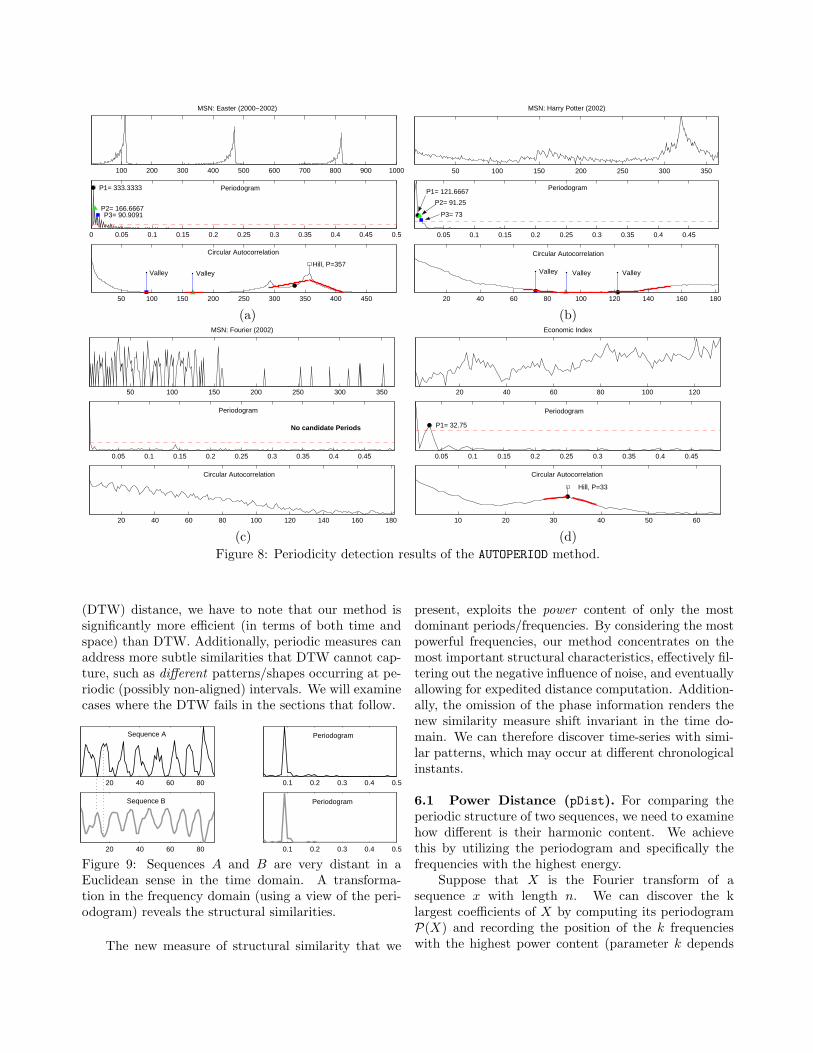
The examples in Figure 8 demonstrate a varietyof situations that might occur when using both theperiodogram and autocorrelation.

Query ‘Easter’(MSN): Examining the demand fora period of 1000 days, we can discover several periodichints above the power threshold in the periodogram.In this example, the autocorrelation information refinesthe original periodogram hint (from 333 → 357). Ad-ditional hints are rejected because they reside on ACFvalleys (in the figure only the top 3 candidate periodsare displayed for reasons of clarity).

Query ‘Harry Potter’(MSN): For the specificquery although there are no observed periodicities (du-ration 365 days), the periodogram returns 3 periodichints, which are mostly attributed to the burst patternduring November when the movie was released. Thehints are classified as spurious upon verification withACF.

Query ‘Fourier’(MSN): This is an example wherethe periodogram threshold effectively does not returncandidate periods. Notice that if we had utilized onlythe autocorrelation information, it would have beenmore troublesome to discover which (if any) periodswere important. This represents another validation thatour choice to perform the period thresholding in thefrequency space was correct.

Economic Index (Stock Market): Finally, this lastsequence from a stock market index illustrates a casewhere both the periodogram and autocorrelation infor-mation concur on the single (albeit weak) periodicity.

Through this experimental testbed we have demon-strated that AUTOPERIOD can provide very accurate pe-riodicity estimates without upsampling the original se-quence. In the sections that follow, we will show howit can be used in conjunction with periodic similaritymeasures, for interactive exploration of sequence data-bases.

6 Structure-Based Similarity and PeriodicMeasures

We introduce structural measures that are based onperiodic features extracted from sequences. Periodicdistance measures can be used for providing moremeaningful structural clustering and visualization ofsequences (whether they are periodic or not). Aftersequences are grouped in ‘periodic’ clusters, using a‘drill-down’ process the user can selectively apply theAUTOPERIOD method for periodicity estimation on thesequences or clusters of interest. In the experimentalsection we provide examples of this methodology usinghierarchical clustering trees.

Let us consider first the utility of periodic distancemeasures with an example. Suppose that one is examin-ing the similarity between the two time-series of Figure9. When sequence A exhibits an upward trend, sequenceB displays a downward drift. Obviously, the Euclideandistance (or inner product) between sequences A andB, will characterize them as very different. However, ifwe exploit the frequency content of the sequences andevaluate their periodogram, we will discover that it isalmost identical. In this new space, the Euclidean dis-tance can easily identify the sequence similarities. Eventhough this specific example could have been addressedin the original space using the Dynamic Time Warping

7

100 200 300 400 500 600 700 800 900 1000

MSN: Easter (2000−2002)

0 0.05 0.1 0.15 0.2 0.25 0.3 0.35 0.4 0.45 0.5

PeriodogramP1= 333.3333

P2= 166.6667P3= 90.9091

50 100 150 200 250 300 350 400 450

Circular Autocorrelation

Hill, P=357ValleyValley

(a)

50 100 150 200 250 300 350

MSN: Harry Potter (2002)

0.05 0.1 0.15 0.2 0.25 0.3 0.35 0.4 0.45

PeriodogramP1= 121.6667

P2= 91.25

P3= 73

20 40 60 80 100 120 140 160 180

Circular Autocorrelation

ValleyValleyValley

(b)

50 100 150 200 250 300 350

MSN: Fourier (2002)

0.05 0.1 0.15 0.2 0.25 0.3 0.35 0.4 0.45

Periodogram

20 40 60 80 100 120 140 160 180

Circular Autocorrelation

No candidate Periods

(c)

20 40 60 80 100 120

Economic Index

0.05 0.1 0.15 0.2 0.25 0.3 0.35 0.4 0.45

Periodogram

P1= 32.75

10 20 30 40 50 60

Circular Autocorrelation

Hill, P=33

(d)

Figure 8: Periodicity detection results of the AUTOPERIOD method.

(DTW) distance, we have to note that our method issignificantly more efficient (in terms of both time andspace) than DTW. Additionally, periodic measures canaddress more subtle similarities that DTW cannot cap-ture, such as different patterns/shapes occurring at pe-riodic (possibly non-aligned) intervals. We will examinecases where the DTW fails in the sections that follow.

20 40 60 80

Sequence A

0.1 0.2 0.3 0.4 0.5

Periodogram

20 40 60 80

Sequence B

0.1 0.2 0.3 0.4 0.5

Periodogram

Figure 9: Sequences A and B are very distant in aEuclidean sense in the time domain. A transforma-tion in the frequency domain (using a view of the peri-odogram) reveals the structural similarities.

The new measure of structural similarity that we

present, exploits the power content of only the mostdominant periods/frequencies. By considering the mostpowerful frequencies, our method concentrates on themost important structural characteristics, effectively fil-tering out the negative influence of noise, and eventuallyallowing for expedited distance computation. Addition-ally, the omission of the phase information renders thenew similarity measure shift invariant in the time do-main. We can therefore discover time-series with simi-lar patterns, which may occur at different chronologicalinstants.

6.1 Power Distance (pDist). For comparing theperiodic structure of two sequences, we need to examinehow different is their harmonic content. We achievethis by utilizing the periodogram and specifically thefrequencies with the highest energy.

Suppose that X is the Fourier transform of asequence x with length n. We can discover the klargest coefficients of X by computing its periodogramP(X) and recording the position of the k frequencieswith the highest power content (parameter k depends

on the desired compression factor). Let us denote thevector holding the positions of the coefficients with thelargest power p+ (so p+ ⊂ [1 . . . n]). To compare xwith any other sequence q, one needs to examine howsimilar energies they carry in the dominant periods ofx. Therefore, we evaluate P(Q(p+)), that describesa sequence holding the equivalent coefficients as thevector P(X(p+)). The distance pDist between thesetwo vectors captures the periodic similarity betweensequences x and q:

pDist = ‖P(Q(p+)) − P(X(p+))‖

Example: Let x and q be two sequences and let theirrespective Fourier Transforms be X = {(1 + 2i), (2 +2i), (1+ i), (5+ i)} and Q = {(2+2i), (1+ i), (3+ i), (1+2i)}. The periodogram vector of X is: P(X) = ‖X‖2 =(5, 8, 2, 26). The vector holding the positions of X withhighest energy is p+ = (2, 4) and therefore P(X(p+)) =(0, 8, 0, 26). Finally, since P(Q) = (8, 2, 10, 5) we havethat: P(Q(p+)) = (0, 2, 0, 5) 2.

In order to meaningfully compare the power contentof two sequences we need to normalize them, so thatthey contain the same amount of total energy. We canassign to any sequence x(n) unit power, by performingthe following normalization:

x(n) =x(n)− 1

N

N�i=1

x(i)�N�

i=1

(x(n)− 1

N

N�i=1

x(i))2

, n = 1, . . . , N

The above transformation will lead to zero mean valueand sum of squared values equal to 1. Parseval’stheorem dictates that the energy in the time domainequals the energy in the frequency domain, thereforethe total energy in the frequency domain should also beunit:

‖x‖2 = ‖F(x)‖2 = 1

After this normalization, we can more meaningfullycompare the periodogram energies.

Indexability: Although in this work we are not goingto discuss now to index the pDist, we would like to notethat this is possible. The representation that we areproposing, utilizes a different set of coefficients for everysequence. While indexing might appear problematicusing space partitioning indices such as R-trees (becausethey operate on a fixed set of dimensions/coefficients),such representations can be easily indexed using metrictree structures, such as VP-Tree or M-Tree (more detailscan be found in [15]).

2The zeros are placed in the vectors for clarity reasons. In the

actual calculations they can be omitted.

7 Periodic Measure Results

We present extensive experiments that show the use-fulness of the new periodic measures and we comparethem with widely used shape based measures or newlyintroduced structural distance measures.

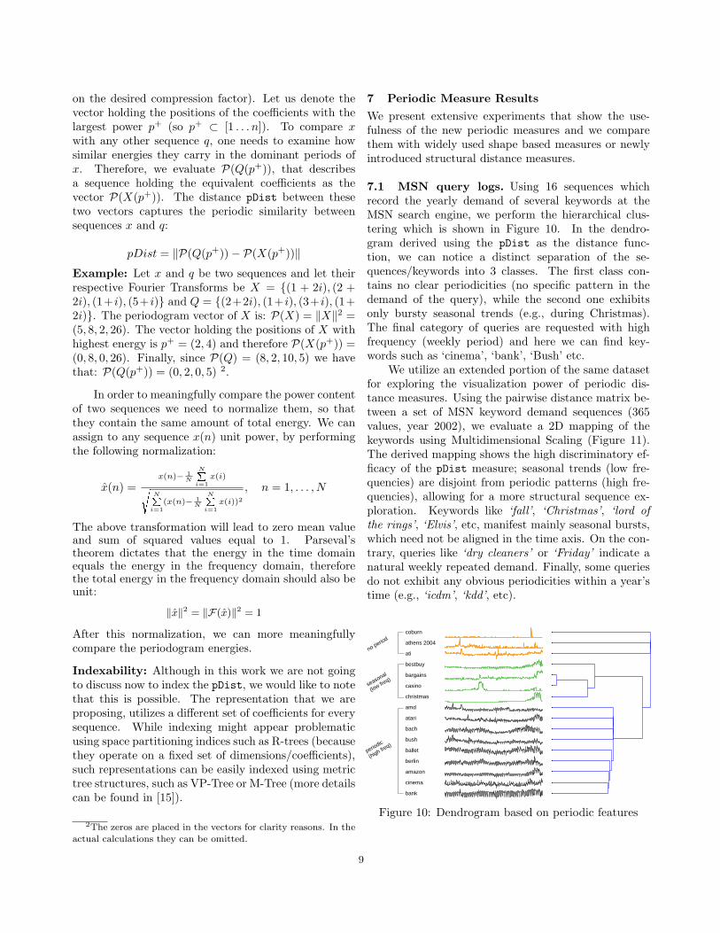
7.1 MSN query logs. Using 16 sequences whichrecord the yearly demand of several keywords at theMSN search engine, we perform the hierarchical clus-tering which is shown in Figure 10. In the dendro-gram derived using the pDist as the distance func-tion, we can notice a distinct separation of the se-quences/keywords into 3 classes. The first class con-tains no clear periodicities (no specific pattern in thedemand of the query), while the second one exhibitsonly bursty seasonal trends (e.g., during Christmas).The final category of queries are requested with highfrequency (weekly period) and here we can find key-words such as ‘cinema’, ‘bank’, ‘Bush’ etc.

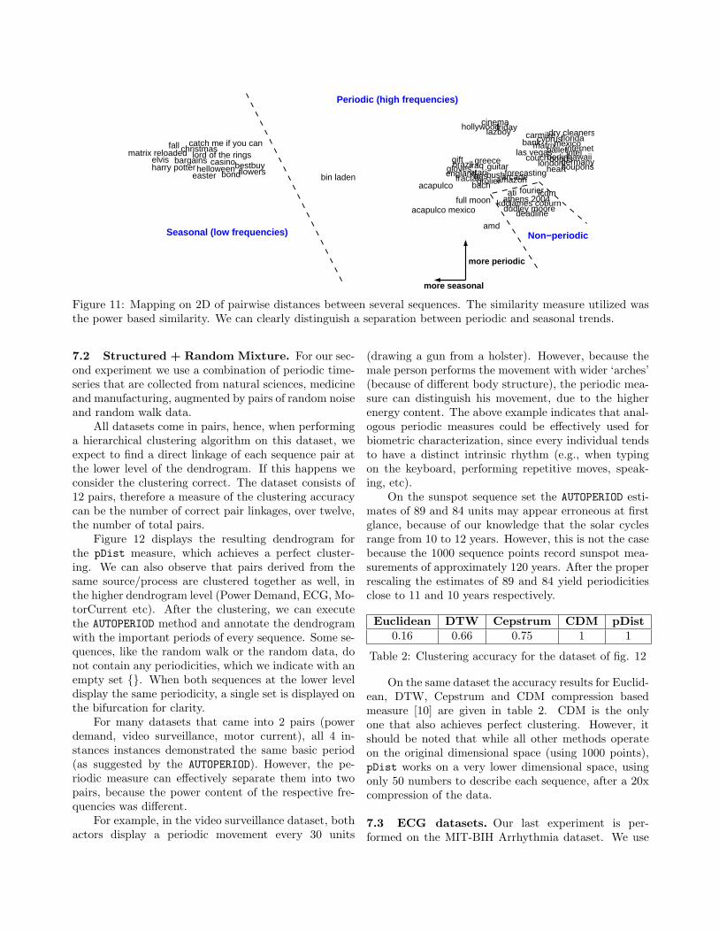
We utilize an extended portion of the same datasetfor exploring the visualization power of periodic dis-tance measures. Using the pairwise distance matrix be-tween a set of MSN keyword demand sequences (365values, year 2002), we evaluate a 2D mapping of thekeywords using Multidimensional Scaling (Figure 11).The derived mapping shows the high discriminatory ef-ficacy of the pDist measure; seasonal trends (low fre-quencies) are disjoint from periodic patterns (high fre-quencies), allowing for a more structural sequence ex-ploration. Keywords like ‘fall’, ‘Christmas’, ‘lord ofthe rings’, ‘Elvis’, etc, manifest mainly seasonal bursts,which need not be aligned in the time axis. On the con-trary, queries like ‘dry cleaners’ or ‘Friday’ indicate anatural weekly repeated demand. Finally, some queriesdo not exhibit any obvious periodicities within a year’stime (e.g., ‘icdm’, ‘kdd’, etc).

bank

cinema

amazon

berlin

ballet

bush

bach

atari

amd

christmas

casino

bargains

bestbuy

ati

athens 2004

coburn

no period

seasonal

(low freq)

periodic

(high freq)

Figure 10: Dendrogram based on periodic features

9

acapulco mexico

acapulcoamazon

amd

arcadearisatari

athens 2004ati

bach

balletbank

bargains berlinbestbuy

bin ladenbond

bondsbrazil

bush

carmike

casino

catch me if you canchristmas

cinema

couchcoupons

cyprus

deadline

dry cleaners

dudley moore

easter

elvis

england

fallflorida

flowers forecasting

fourierfractals

friday

full moon

germanygiftgloves

greece

grolier

guitarharry potterhawaii

hearthelloween

hollywood

icdm

intelinternet

iraq

james coburnkdd

las vegas

lazboy

londonlord of the ringsmatrix reloaded

matrixmexico

Seasonal (low frequencies)

Periodic (high frequencies)

Non−periodic

more periodic

more seasonal

Figure 11: Mapping on 2D of pairwise distances between several sequences. The similarity measure utilized wasthe power based similarity. We can clearly distinguish a separation between periodic and seasonal trends.

7.2 Structured + Random Mixture. For our sec-ond experiment we use a combination of periodic time-series that are collected from natural sciences, medicineand manufacturing, augmented by pairs of random noiseand random walk data.

All datasets come in pairs, hence, when performinga hierarchical clustering algorithm on this dataset, weexpect to find a direct linkage of each sequence pair atthe lower level of the dendrogram. If this happens weconsider the clustering correct. The dataset consists of12 pairs, therefore a measure of the clustering accuracycan be the number of correct pair linkages, over twelve,the number of total pairs.

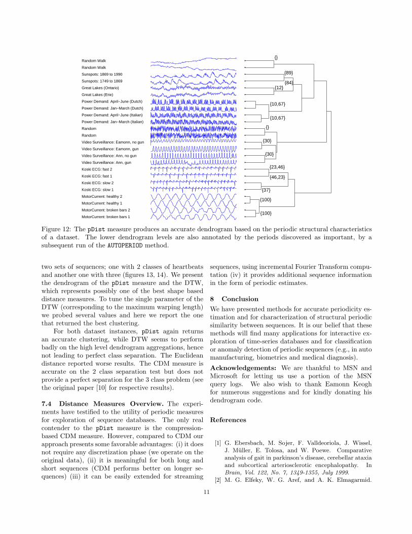
Figure 12 displays the resulting dendrogram forthe pDist measure, which achieves a perfect cluster-ing. We can also observe that pairs derived from thesame source/process are clustered together as well, inthe higher dendrogram level (Power Demand, ECG, Mo-torCurrent etc). After the clustering, we can executethe AUTOPERIOD method and annotate the dendrogramwith the important periods of every sequence. Some se-quences, like the random walk or the random data, donot contain any periodicities, which we indicate with anempty set {}. When both sequences at the lower leveldisplay the same periodicity, a single set is displayed onthe bifurcation for clarity.

For many datasets that came into 2 pairs (powerdemand, video surveillance, motor current), all 4 in-stances instances demonstrated the same basic period(as suggested by the AUTOPERIOD). However, the pe-riodic measure can effectively separate them into twopairs, because the power content of the respective fre-quencies was different.

For example, in the video surveillance dataset, bothactors display a periodic movement every 30 units

(drawing a gun from a holster). However, because themale person performs the movement with wider ‘arches’(because of different body structure), the periodic mea-sure can distinguish his movement, due to the higherenergy content. The above example indicates that anal-ogous periodic measures could be effectively used forbiometric characterization, since every individual tendsto have a distinct intrinsic rhythm (e.g., when typingon the keyboard, performing repetitive moves, speak-ing, etc).

On the sunspot sequence set the AUTOPERIOD esti-mates of 89 and 84 units may appear erroneous at firstglance, because of our knowledge that the solar cyclesrange from 10 to 12 years. However, this is not the casebecause the 1000 sequence points record sunspot mea-surements of approximately 120 years. After the properrescaling the estimates of 89 and 84 yield periodicitiesclose to 11 and 10 years respectively.

Euclidean DTW Cepstrum CDM pDist0.16 0.66 0.75 1 1

Table 2: Clustering accuracy for the dataset of fig. 12

On the same dataset the accuracy results for Euclid-ean, DTW, Cepstrum and CDM compression basedmeasure [10] are given in table 2. CDM is the onlyone that also achieves perfect clustering. However, itshould be noted that while all other methods operateon the original dimensional space (using 1000 points),pDist works on a very lower dimensional space, usingonly 50 numbers to describe each sequence, after a 20xcompression of the data.

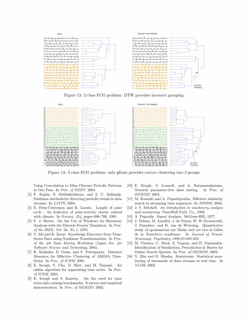
7.3 ECG datasets. Our last experiment is per-formed on the MIT-BIH Arrhythmia dataset. We use

MotorCurrent: broken bars 1

MotorCurrent: broken bars 2

MotorCurrent: healthy 1

MotorCurrent: healthy 2

Koski ECG: slow 1

Koski ECG: slow 2

Koski ECG: fast 1

Koski ECG: fast 2

Video Surveillance: Ann, gun

Video Surveillance: Ann, no gun

Video Surveillance: Eamonn, gun

Video Surveillance: Eamonn, no gun

Random

Random

Power Demand: Jan−March (Italian)

Power Demand: April−June (Italian)

Power Demand: Jan−March (Dutch)

Power Demand: April−June (Dutch)

Great Lakes (Erie)

Great Lakes (Ontario)

Sunspots: 1749 to 1869

Sunspots: 1869 to 1990

Random Walk

Random Walk {}

{89}

{84} {12}

{10,67}

{10,67}

{}

{30}

{30}

{23,46}

{46,23}

{37}

{100}

{100}

Figure 12: The pDist measure produces an accurate dendrogram based on the periodic structural characteristicsof a dataset. The lower dendrogram levels are also annotated by the periods discovered as important, by asubsequent run of the AUTOPERIOD method.

two sets of sequences; one with 2 classes of heartbeatsand another one with three (figures 13, 14). We presentthe dendrogram of the pDist measure and the DTW,which represents possibly one of the best shape baseddistance measures. To tune the single parameter of theDTW (corresponding to the maximum warping length)we probed several values and here we report the onethat returned the best clustering.

For both dataset instances, pDist again returnsan accurate clustering, while DTW seems to performbadly on the high level dendrogram aggregations, hencenot leading to perfect class separation. The Euclideandistance reported worse results. The CDM measure isaccurate on the 2 class separation test but does notprovide a perfect separation for the 3 class problem (seethe original paper [10] for respective results).

7.4 Distance Measures Overview. The experi-ments have testified to the utility of periodic measuresfor exploration of sequence databases. The only realcontender to the pDist measure is the compression-based CDM measure. However, compared to CDM ourapproach presents some favorable advantages: (i) it doesnot require any discretization phase (we operate on theoriginal data), (ii) it is meaningful for both long andshort sequences (CDM performs better on longer se-quences) (iii) it can be easily extended for streaming

sequences, using incremental Fourier Transform compu-tation (iv) it provides additional sequence informationin the form of periodic estimates.

8 Conclusion

We have presented methods for accurate periodicity es-timation and for characterization of structural periodicsimilarity between sequences. It is our belief that thesemethods will find many applications for interactive ex-ploration of time-series databases and for classificationor anomaly detection of periodic sequences (e.g., in automanufacturing, biometrics and medical diagnosis).

Acknowledgements: We are thankful to MSN andMicrosoft for letting us use a portion of the MSNquery logs. We also wish to thank Eamonn Keoghfor numerous suggestions and for kindly donating hisdendrogram code.

References

[1] G. Ebersbach, M. Sojer, F. Valldeoriola, J. Wissel,J. Muller, E. Tolosa, and W. Poewe. Comparativeanalysis of gait in parkinson’s disease, cerebellar ataxiaand subcortical arteriosclerotic encephalopathy. InBrain, Vol. 122, No. 7, 1349-1355, July 1999.

[2] M. G. Elfeky, W. G. Aref, and A. K. Elmagarmid.

11

1

8

10

4

5

7

9

3

2

6

11

19

13

12

14

20

15

17

18

16

pDist

1

4

10

2

6

5

7

8

9

3

11

15

19

12

14

16

13

17

20

18

IncorrectGrouping

Dynamic Time Warping

Figure 13: 2 class ECG problem: DTW provides incorrect grouping

146103951172812132115141622241719202318252931303432262728333536

pDist

158124102369711141618151922202313172124252932283136262735303334

Dynamic Time Warping

IncorrectGrouping

Figure 14: 3 class ECG problem: only pDist provides correct clustering into 3 groups

Using Convolution to Mine Obscure Periodic Patternsin One Pass. In Proc. of EDBT, 2004.

[3] F. Ergun, S. Muthukrishnan, and S. C. Sahinalp.Sublinear methods for detecting periodic trends in datastreams. In LATIN, 2004.

[4] E. Friss-Cristensen and K. Lassen. Length of solarcycle - An Indicator of solar-activity closely relatedwith climate. In Science, 254, pages 698–700, 1991.

[5] F. J. Harris. On the Use of Windows for HarmonicAnalysis with the Discrete Fourier Transform. In Proc.of the IEEE, Vol. 66, No 1, 1978.

[6] T. Ide and K. Inoue. Knowledge Discovery from Time-Series Data using Nonlinear Transformations. In Proc.of the 4th Data Mining Workshop (Japan Soc. forSoftware Science and Technology, 2004.

[7] K. Kalpakis, D. Gada, and V. Puttagunta. DistanceMeasures for Effective Clustering of ARIMA Time-Series. In Proc. of ICDM, 2001.

[8] E. Keogh, S. Chu, D. Hart, and M. Pazzani. Anonline algorithm for segmenting time series. In Proc.of ICDM, 2001.

[9] E. Keogh and S. Kasetty. On the need for timeseries data mining benchmarks: A survey and empiricaldemonstration. In Proc. of SIGKDD, 2002.

[10] E. Keogh, S. Lonardi, and A. Ratanamahatana.Towards parameter-free data mining. In Proc. ofSIGKDD, 2004.

[11] M. Kontaki and A. Papadopoulos. Efficient similaritysearch in streaming time sequences. In SSDBM, 2004.

[12] J. S. Mitchell. An introduction to machinery analysisand monitoring. PennWell Publ. Co., 1993.

[13] A. Papoulis. Signal Analysis. McGraw-Hill, 1977.[14] J. Tulena, M. Azzolini, J. de Vriesa, W. H. Groeneveld,

J. Passchier, and B. van de Wetering. Quantitativestudy of spontaneous eye blinks and eye tics in Gillesde la Tourette’s syndrome. In Journal of Neurol.Neurosurg. Psychiatry 1999,67:800-802.

[15] M. Vlachos, C. Meek, Z. Vagena, and D. Gunopulos.Identification of Similarities, Periodicities & Bursts forOnline Search Queries. In Proc. of SIGMOD, 2004.

[16] Y. Zhu and D. Shasha. Statstream: Statistical mon-itoring of thousands of data streams in real time. InVLDB, 2002.