On-Orbit Structural Dynamics Performance of the Roll-Out Solar Array

Matthew K. Chamberlain1 NASA Langley Research Center, Hampton VA 23681

Steven H. Kiefer2 Deployable Space Systems, Santa Barbara, CA 93111

and Jeremy A. Banik3

Air Force Research Laboratory, Space Vehicle Directorate, Kirtland AFB, NM 87117

The Roll-Out Solar Array (ROSA) flight experiment was launched to the International Space Station (ISS) on June 3rd, 2017. ROSA is an innovative, lightweight solar array with a flexible substrate that makes use of the stored strain energy in its composite structural members to provide deployment without the use of motors. This paper will discuss the results of various structural dynamics experiments conducted on the ISS during the weeks following launch. Data gathered from instrumentation on the solar array wing during the experiments are compared with pre-flight predictions from two different finite element modeling efforts. Two distinct methods were used to reconstruct the modal characteristics of ROSA from the data collected on orbit. Of particular interest in this effort are the first few system modes and mode shapes of the array, the amount of structural damping present, and degree of structural-thermal interaction seen during eclipse exit. Discrepancies between the behavior predicted by the models and that observed on orbit are identified and discussed. The goal in this effort was to better understand the performance of ROSA and to improve modeling efforts for future designs of similar solar arrays.

I. I. Introduction OMMERCIAL and governmental activities in space demand increases in electrical power at a low mass and volume penalty. For this reason, the Air Force Research Laboratory (AFRL), the National Aeronautics and Space

Administration (NASA), and Deployable Space Systems, Inc. (DSS), developed the Roll-Out Solar Array (ROSA) as a lightweight alternative to conventional rigid panel solar arrays. AFRL and the Department of Defense (DoD) Space Test Program led the development of a 5.40 meter long by 1.67 meter wide experimental ROSA wing that was launched to the International Space Station (ISS) on the SpaceX Falcon 9 Commercial Resupply Services mission (CRS-11) on June 3rd, 2017. After two weeks in space, ROSA was removed from the depressurized trunk portion of the Dragon capsule using the ISS Special Purpose Dexterous Manipulator (SPDM), and positioned for deployment as seen in Fig. 1. Over the next seven days, ROSA was the subject of a series of experiments to measure its functionality in the extreme temperatures and micro-gravity of orbital flight. Following deployment on the first day of experimentation, four and a half days of structural dynamics tests were carried out, followed by tests of the performance of photovoltaics. A vast amount of data was gathered and will be compared to analytical predictions of deployment, forced vibration response, eclipse exit thermal-structural response, and power production. A detailed description of the ROSA experiment flight operations can be found in Refs. [1-6]. This work focuses on the structural dynamics results of the wing on-orbit.

ROSA consists of a pair of longitudinally-oriented high-strain-composite slit tube booms attached at their tip to a mandrel and at their root to a yoke and spacecraft adapter. The booms are pre-tensioned by the Integrated Modular Blanket Assembly (IMBA), consisting of lightweight photovoltaic power modules attached to mesh and connected at 1 Research Aerospace Engineer, Structural Dynamics Branch, 4B West Taylor St, AIAA Senior Member 2 Structural Analyst, 460 Ward Dr, AIAA Member 3 Senior Research Engineer, 3550 Aberdeen Avenue SE, AIAA Associate Fellow

C

https://ntrs.nasa.gov/search.jsp?R=20190000446 2020-03-25T03:54:02+00:00Z

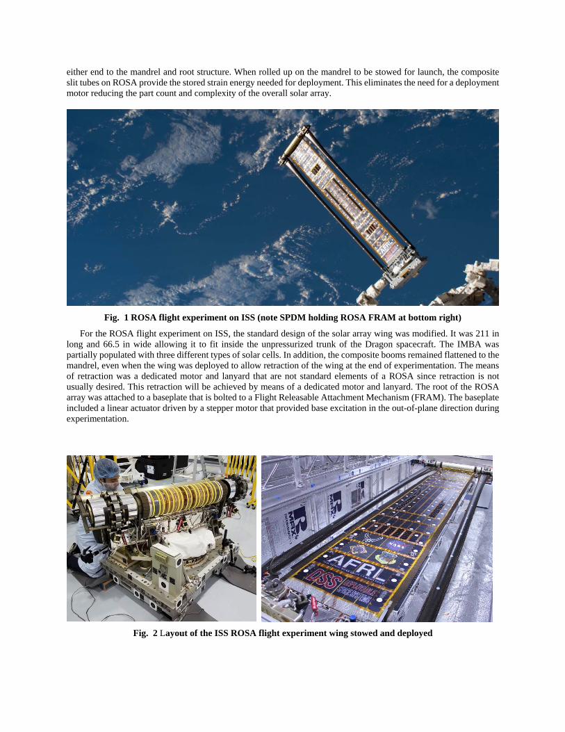
either end to the mandrel and root structure. When rolled up on the mandrel to be stowed for launch, the composite slit tubes on ROSA provide the stored strain energy needed for deployment. This eliminates the need for a deployment motor reducing the part count and complexity of the overall solar array.

Fig. 1 ROSA flight experiment on ISS (note SPDM holding ROSA FRAM at bottom right)

For the ROSA flight experiment on ISS, the standard design of the solar array wing was modified. It was 211 in long and 66.5 in wide allowing it to fit inside the unpressurized trunk of the Dragon spacecraft. The IMBA was partially populated with three different types of solar cells. In addition, the composite booms remained flattened to the mandrel, even when the wing was deployed to allow retraction of the wing at the end of experimentation. The means of retraction was a dedicated motor and lanyard that are not standard elements of a ROSA since retraction is not usually desired. This retraction will be achieved by means of a dedicated motor and lanyard. The root of the ROSA array was attached to a baseplate that is bolted to a Flight Releasable Attachment Mechanism (FRAM). The baseplate included a linear actuator driven by a stepper motor that provided base excitation in the out-of-plane direction during experimentation.

Fig. 2 Layout of the ISS ROSA flight experiment wing stowed and deployed

Prior to launch, a ROSA engineering demonstration unit (EDU) was constructed and tested in thermal vacuum conditions to establish a structural dynamics baseline response. In addition, AFRL, NASA, and DSS carried out extensive modeling and simulation. Models were correlated with ground test data and used to develop predictions for performance in space. In this paper, the results of those predictions were compared with data gathered during experimentation on-orbit. Some of this data was analyzed in real-time during flight, while higher-frequency data was stored, downloaded, and processed for a more thorough analysis at a later date. The remainder of this paper describes the instrumentation of the wing, the types of experiments that were run while the solar array wing was in space, some anomalous behavior noted during flight, and how the experimental data compares with analytical models.

II. Instrumentation, Data Collection, and Processing

During experiments, data relevant to the dynamics of the array was gathered from ROSA in two ways: from a handful of accelerometers located at key points, and from video of photogrammetry targets scattered extensively over the entire structure. As seen in Fig. 3, one-axis accelerometers were located at the center and both edges of the IMBA blanket at the middle of its length to capture blanket modes. Similarly, accelerometers were located at the center and ends of the mandrel in order to capture wing structure modes. Two other accelerometers were placed at the roots of the booms, providing the data sources closest to the input signal. Finally, a tri-axial accelerometer was placed on the experimental base plate below the linear actuator to monitor the state of the base of the experiment where it interfaced with the robot arm. All the single axis accelerometers were oriented to measure movement out of the plane of the array.

Fig. 3 Instrumentation included on deployed ROSA solar array wing

As seen in Fig. 3, the entire wing, including the booms and IMBA, was marked with reflective photogrammetry

targets. Other targets not shown in Fig. 3 were located on the opposite side of the stabilizer, at various points on the root structure, and the FRAM. The position of the SPDM throughout the week of experimentation was chosen so that it could be viewed from the maximum number of stationary cameras located on the exterior of the space station. In addition, the ROSA wing root structure includes three cameras for verification of deployment and retraction. During key experiments, video feeds from four to five views available from the ROSA and ISS cameras were recorded so that the results of later photogrammetric analysis can be compared with data gathered from accelerometers.

The structural dynamics experiments generated a huge amount of data, requiring a system for managing it. While resistance temperature detectors and accelerometers on ROSA recorded data at 200 Hz, saving it to solid state hard drives, the data could only be downloaded in real-time from ISS at a rate of 20 Hz. This data was passed through a real-time data analysis tool that displayed raw and filtered time histories of the accelerometers during each run (see

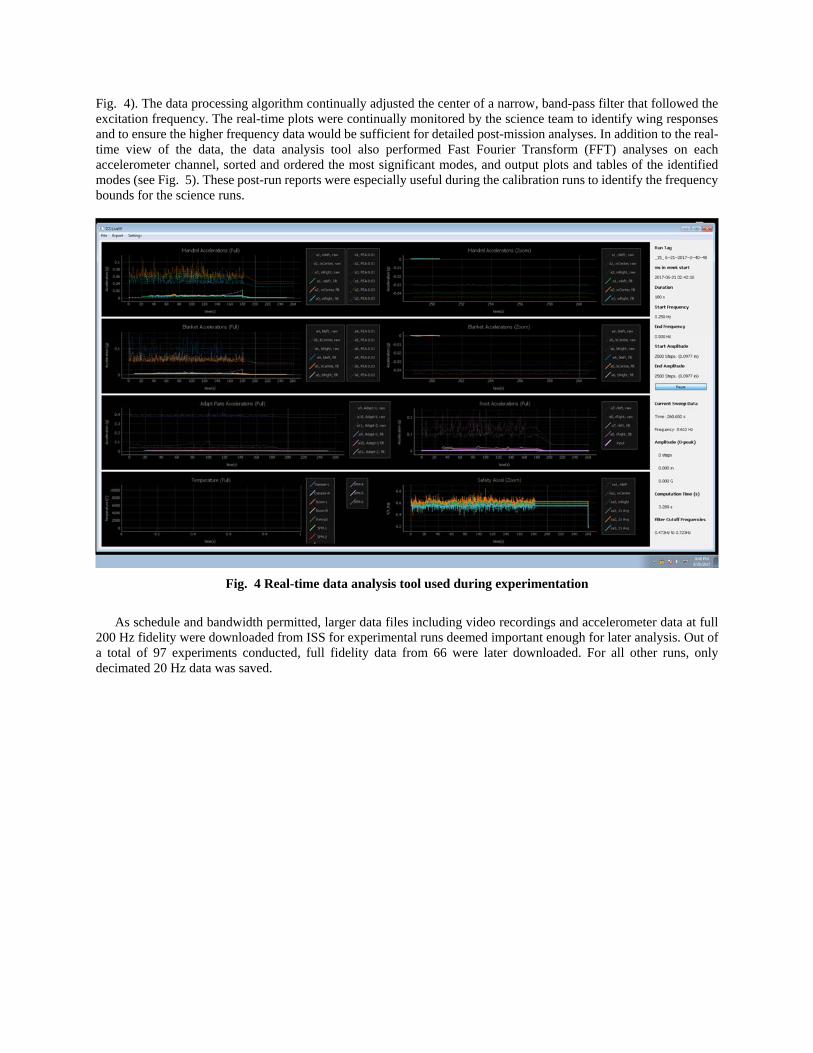
Fig. 4). The data processing algorithm continually adjusted the center of a narrow, band-pass filter that followed the excitation frequency. The real-time plots were continually monitored by the science team to identify wing responses and to ensure the higher frequency data would be sufficient for detailed post-mission analyses. In addition to the real-time view of the data, the data analysis tool also performed Fast Fourier Transform (FFT) analyses on each accelerometer channel, sorted and ordered the most significant modes, and output plots and tables of the identified modes (see Fig. 5). These post-run reports were especially useful during the calibration runs to identify the frequency bounds for the science runs.

Fig. 4 Real-time data analysis tool used during experimentation

As schedule and bandwidth permitted, larger data files including video recordings and accelerometer data at full

200 Hz fidelity were downloaded from ISS for experimental runs deemed important enough for later analysis. Out of a total of 97 experiments conducted, full fidelity data from 66 were later downloaded. For all other runs, only decimated 20 Hz data was saved.

Fig. 5 Sample of quick-look analysis for one data run

III. On-Orbit Experiments The ROSA flight experiment on ISS had a number of scientific objectives, including demonstration of deployment

and photovoltaic performance, but the bulk of the time spent in space was used to try to characterize the structural dynamics of the solar array in microgravity under different conditions. Of particular interest was data that could be used to identify and characterize the first few bending modes of the array. Because of the nature of ROSA, it has both structural modes that one might expect from a long flat object, and distinct blanket modes due to the tensioned IMBA “blanket” held between the structure. Model predictions prior to flight suggested that several structural and blanket modes would occur below 3 Hz. These low frequency structure and blanket modes were the focus of the dynamics experimentation described in the next subsections.

A. Sine Sweeps In order to excite out of plane motion in the solar array structure, a linear actuator driven by a stepper motor was

included in the ROSA flight experiment and located between the root of the solar array and the FRAM to which it was attached. The actuator was pre-programmed to apply sinusoidal motion for a given period of time at a given amplitude and to sweep between two frequencies. For each experimental run, the duration, amplitude, and frequency range were manually updated based on the interpretation of the most recent prior runs. Model predictions prior to flight suggested that this arrangement could excite a number of key modes below 3 Hz including both structural and blanket modes.

The plan for experimentation prior to launch called for initial “calibration” testing to make use of sine sweeps over a wide range of frequencies to see whether the structural responses of ROSA seen in accelerometer data corresponded with FEM predictions. Once modes were identified, sine sweeps over much smaller frequency ranges would be repeated five times during both daylight and night conditions to gather a suite of high quality “science” data. Under the initial plan, something on the order of 30 sine sweeps would have been carried out.

During experimentation at ISS, real-time analysis of the results indicated the presence of two unexpected phenomena that required a much longer period of sine sweep calibration than was planned. As a result, 97 sine sweep

runs were carried out, most lasting three to five minutes. After refinement, sets of five day and five night runs were carried out for each of three frequency ranges described in Table 1.

Table 1 Sine sweep settings for dynamics science runs

Frequency Range (Hz) Amplitude (Motor Steps) Excitation Duration (sec) Rationale 0.37 – 0.41 2500 180 Excite 1st bending mode of whole array 0.50 – 1.25 1200 300 Excite various low frequency blanket modes 1.50 – 2.00 800 300 Excite various higher order blanket modes

A large amount of high quality data was generated outside the 30 “science” runs described in Table 1, so the results from many of the runs needed to calibrate the frequency range were downloaded at full fidelity for further analysis.

B. Free Decay Tests The free decay of the wing in vacuum was tested by continuing to record data from accelerometers for up to a

minute after base excitation had concluded. In addition, several efforts were made to excite the solar array by driving its base at a frequency near a mode identified in preliminary calibration experiments. After a few seconds of excitation, the base drive was eliminated but data recording continued in an effort to capture a bigger initial response.

C. Eclipse Exit Tests During a number of orbits, the accelerometers in the ROSA wing were recording data as the wing either exited

eclipse and was warmed by direct sunlight, or entered darkness and rapidly cooled down. Data was recorded five times in each of these conditions to verify the extent of any thermal-structural deflections in the wing. Since the slit tube booms and IMBA blanket were made with low coefficient of thermal expansion (CTE) materials, these deflections were expected to be small.

IV. Pre-Flight Modeling and Analysis Prior to flight, two separate finite modeling efforts were undertaken in an effort to predict the dynamics of ROSA.

The efforts produced two distinct wing models with differing assumptions that are described below: An Ansys FEM (See Fig. 6a) was developed which included pre-integrated shell properties for the booms

and a stiffness-scaled shell representation of the IMBA flex blanket. The booms were initially modeled as flat and the thermal force vectors of the pre-integrated boom properties were chosen to develop a final curvature of 2in (4in diameter) when an appropriate uniform thermal load was applied with the booms unrestrained. In the deployed model, the tip of the booms were constrained flat against the mandrel. Upon exposure to the appropriate thermal load, the transition zone developed. Modal & harmonic dynamics analyses were performed after the boom & IMBA pre-stress steps were completed. 

An Abaqus model (See Fig. 6b) was constructed around a two-step analysis procedure. In the first step, an explicit simulation was used to model the precise distortion of the slit tube booms to their shape when rolled against the mandrel. In the second step, the booms’ configurations were imported into an implicit analysis to pre-tension the array, calculate modes, and generate dynamic responses. One key difference between this model and the Ansys model was that the IMBA blanket was modeled as a mesh of beams instead of membrane. It also ignoreed all of the hardware below the root structure of the wing.

In order to check the general assumptions made in each model, modified versions of each were used to predict the performance of the wing during ground testing. For the flight version of the wing, each model was used to predict modes as well as mode shapes as shown in Table 2 and Fig. 7, and to predict response at accelerometer locations for various damping values.

a.) b.)

Fig. 6 Finite element models developed in a.) ANSYS and b.) Abaqus

Table 2 Summary of ROSA modes and mode shapes from finite element models

Abaqus Model ANSYS Model

Mode Frequency (Hz) Shape Mode Frequency (Hz) Shape 1 0.50 Structural Bending 1 0.54 Structural Bending

2 0.64 Structural Torsion 2 0.66 Structural Torsion

3 0.98 Blanket Drum 3 0.91 Blanket Torsion

4 1.24 Blanket Torsion 4 0.93 Blanket Saddle

5 1.88 2nd

Order Blanket Drum 5 0.94 Blanket Drum

6 2.22 Lead-Lag in Plane 6 1.12 2nd

Order Lateral Blanket Drum

7 1.49 3rd

Order Lateral Blanket Drum 8 1.78 2nd Order Blanket Twist

9 1.79 2nd Order Blanket Drum

10 1.82 2nd Order Blanket Saddle

11 1.87 Lead-Lag in Plane

12 2.00 3rd Order Blanket Twist

13 2.06 4th Order Lateral Blanket Drum

Fig. 7 Summary of ROSA FEM modes and mode shapes from both models

V. Results During experimentation on ISS, some blanket modes were obvious both in video streamed by cameras on station,

and in the decimated 20 Hz accelerometer data downlinked and analyzed in real time. Blanket modes seemed to be easily excited at frequencies starting around 0.6 Hz and would oscillate even after excitation stopped. This first blanket mode was lower than expected and did not have a shape predicted by finite element models prior to flight. However, the structural or mandrel mode was not as easily excited, appeared to be highly damped, and its frequency was significantly lower than expected. Extensive post-flight analysis was needed to find an explanation for these results.

An extraordinary amount of data was generated during experimentation on ISS. This data was downloaded at its original 200 Hz sampling rate and cut down into data sets associated with each experimental run based on the recorded times at which each run started and began. At first, the data appeared noisy and inconsistent, as vibrations from the stepper motor driving the experiment’s linear actuator were clearly visible. Early attempts to apply a single filtering scheme to all the accelerometers did not work well, however by plotting the peaks from FFTs of each accelerometer from each experimental run as in Fig. 8, clear trends were evident.

Eventually, two means of identifying the system’s modes, damping, and mode shapes were found. First, an accelerometer-specific approach was used to filter the data from each source in an effort to identify modes in the excitation and decay phases of each run. This approach led to proximate frequencies for several modes, damping for the primary structural and blanket modes, and an indication of which mode shapes were present at each frequency. To check these results, the Eigensystem Realization Algorithm [7, 8] was used to find a set of modes, mode shapes, and damping that best fit all of the accelerometer data simultaneously for each run. These results were aggregated over all the runs analyzed to identify the most common system modes, as discussed in the following subsections.

Fig. 8 FFT peaks from excitation phase of all data runs

A. Individual Accelerometer Analysis The individual accelerometer analysis consisted of two algorithms. The first was developed to identify significant

modes and associated trends with various run properties. The second was developed to determine the damping of significant modes during the free-decay portion of each run. The algorithms were automated in order to process the significant number of accelerometer data sets. Many accelerometer data sets included multiple modes in each run, often independent from modes found in the other accelerometer data sets of the same run. This general approach to the data processing ensured that the modes found were not constrained to expectations or limited to sets where accelerometer data was consistent.

Prior to applying the mode algorithm, each of 33 science run data sets were split into ‘during excitation’ and ‘free decay’ set. An FFT analysis of each of these accelerometer data sets was performed. The frequency data was then truncated to a range between 0.1 Hz and 3.0 Hz. A peak-finding routine was then employed on the frequency domain data to identify up to three significant and independent modes. The mode amplitude in acceleration and displacement were computed from the magnitude of the FFT results. While these values do not represent the actual motion of the hardware, they provide a good means of mode strength comparison between data sets. The mode values and amplitudes, along with excitation type, run ID, average SPM temperature, and average boom temperature for each run was recorded. An example of the results gathered for one run is shown in Fig. 9. After the 33 data sets were analyzed, a total of 1,039 modes from all 11 accelerometers were found.

Fig. 9 Example of the modal algorithm FFT analysis with significant modes indicated

The damping algorithm was applied to the free-decay portion of the 33 data sets and began with the same steps as

the mode algorithm. Once modes of each accelerometer were identified, a high pass filter with a cutoff frequency of 0.1 Hz was applied to remove any static/DC offset present. The high pass filtered data included significant mechanical noise from the drive mechanisms. A bandpass filter was then applied to the individual accelerometer data which was centered on the mode and included a bandwidth equal to 10% of the mode frequency. Damping was computed for both the positive and negative peak amplitudes by fitting a logarithmic curve to local peaks of the band-past filtered data using a least-squares curve fitting method. In some runs, the time period considered was limited to regions of the data that exhibited significant decay. After damping was computed the Pearson’s R fit value was computed for the bandpass filtered data compared to the high-pass filtered data. A relatively high Pearson’s R value (>0.3) indicated the bandpass filtered data represented a significant portion of the unfiltered data. Only damping computed from runs with relatively high Pearson’s R values were included in the damping summary. The average damping, log fit, and Pearson’s R value was recorded in addition to the run parameters recorded in the mode algorithm. Damping was computed for a total of 972 modes.

a) b)

Fig. 10 Example of the damping algorithm a) log decrement analysis and b) the Pearson’s R fit visualized

Interactive data plotting tools were developed in order to visualize the results from the modal and damping

algorithms and discern trends in the summarized data. The tools were similar for both data sets and produced scatter plots of any recorded parameter versus another (e.g. amplitude versus frequency) for the entire data set. The resulting scatter plots of the modal data set provide a means of identifying modes through clusters of points at similar frequencies and accelerations, as shown in Fig. 11, where transparency is based on how low the acceleration of each mode is. The interactive data plot tools were used to identify bands of frequencies that represented individual modes. The excitation data set was then partitioned to these bands. Box plots were generated for the distribution of frequencies within the bands. The size of the box is the interquartile range (Q1-Q3) with whiskers extending up to 1.5x the interquartile range for each box. Data points outside of the whiskers are considered outliers and are plotted as open circles as shown in Fig. 12, the scatter of the modes within these bands was fairly tight, indicating unique modes exist in those ranges. The modes identified in this manner and the most active accelerometer for each mode are listed in Table 3.

Fig. 11 Example of use of the interactive scatter plot tool for the modal data set

Fig. 12 Mode frequency distribution for the excitation data set

Table 3 Approximate modes and shapes found using per-accelerometer approach to excitation data

Mode Approximate Frequency (Hz) Shape or Most Active Accelerometer 1 0.40 Structural bending 2 0.62 Right blanket edge 3 0.81 Left blanket edge 4 0.91 Center blanket 5 1.20 Center blanket 6 1.70 Right blanket edge 7 1.80 Right blanket edge 8 2.0 Center & left blanket

In addition to identifying significant modes, the scatter tool was also used to identify trends in the data sets such as changes in mode with temperature. For example, the blanket center mode appeared to shift from ~0.9 Hz in sunlight to ~1.2 Hz when in eclipse (see Fig. 13). Another observation was that the blanket left mode at ~0.8 Hz was more pronounced when in eclipse.

Fig. 13 Example of use of the interactive scatter plot tool highlighting trends in the modes with temperature

The free-decay data set was partitioned into the same bands of frequencies as the excitation data set. The data set was filtered to include only damping and frequency data for traces with a Pearson’s R fit > 0.3 and plotted as shown in Fig. 14. The clustering of data along the horizontal axis in this plot indicates a significant free-decay mode. Box plots were generated for both the mode frequencies and the damping values (see Fig. 15 and Fig. 16). The size of the box is the interquartile range (Q1-Q3) with whiskers extending up to 1.5x the interquartile range for each box. Data points outside of the whiskers were considered outliers and plotted as open circles. The mean mode frequencies and damping values are shown in Table 4.

Fig. 14 Example of use of the interactive scatter plot tool for the damping data set

Fig. 15 Mode frequency distribution in the free-decay data set

Fig. 16 Damping distribution in the free-decay data set

Table 4 Mean frequency and damping found using the per-accelerometer approach to free-decay data

Mode Mean Frequency (Hz) Mean Damping (%) 1 0.41 2.5 2 0.62 6.1 3 0.82 0.7 4 0.91 1.1 5 1.21 1.0 6 1.71 0.7 7 1.80 0.5 8 2.07 1.3

B. Eigenvalue Realization Algorithm Analysis The single-accelerometer approach provided strong indications of the locations of a number of modes below 2 Hz,

their damping, and an idea of what the mode shapes associated with them might be. To check these results, a second approach was utilized. For each of 46 data runs for which a full set of 200 Hz data was available without any dropouts, the Eigenvalue Realization Algorithm (ERA) [7, 8] was used to carry out modal identification, producing likely system modes, their damping, and the shapes associated with them. As a first pass, ERA was used in its free decay and time domain settings with a suggested 200 modes below 100 Hz. The clusters of modes at certain frequencies in the results shown in Fig. 17 are suggestive of modes at around 0.4 Hz, 0.8 Hz, 0.9 Hz, 1.1 Hz, and 1.7 Hz. There are is also a cluster of data suggesting at least one mode in the area between 0.6 and 0.7 Hz.

Fig. 17 Quick ERA assessment of mode locations in experimental runs

Next, a full assessment of each experimental run using ERA was carried out using data that had been low-pass filtered at 10 Hz to focus on content in the range of the modes of interest. For each run, the accelerometers at the roots of the booms were treated as inputs, while those on the mandrel and blanket were treated as outputs. ERA was run repeatedly for each mode, identifying systems with 10 to 30 modes. The result of this effort was a set of 21 system models for each run. Ideally, every system model would contain identical modes but they tend to contain some variability. To find the most likely modes for each experimental run, the modes for the 21 system models were ranked according to how often they appeared with similar damping (less than 20% change between models), similar frequency (less than 10% change between models), and similar mode shape (Modal Assurance Criterion of greater than 0.9.)

The result of this approach was that for each experimental run, a list of modes was generated. Each mode in the list was judged proximate in that it showed up consistently in models with similar features. While this approach generated similar sets of modes between different experimental runs, the estimated damping for the runs varied greatly, suggesting poor model fit overall.

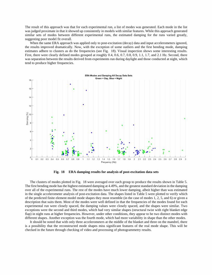
When the same ERA approach was applied only to post-excitation (decay) data and input accelerometers ignored, the results improved dramatically. Now, with the exception of some outliers and the first bending mode, damping estimates adhere to clusters as do the frequencies (see Fig. 18). Visual inspection shows some interesting results. First, there were clearly defined modes grouped at roughly 0.4, 0.6, 0.7, 0.8, 0.9, 1.1, 1.7, and 2.1 Hz. Second, there was separation between the results derived from experiments run during daylight and those conducted at night, which tend to produce higher frequencies.

Fig. 18 ERA damping results for analysis of post-excitation data sets

The clusters of modes plotted in Fig. 18 were averaged over each group to produce the results shown in Table 5. The first bending mode has the highest estimated damping at 4.49%, and the greatest standard deviation in the damping over all of the experimental runs. The rest of the modes have much lower damping, albeit higher than was estimated in the single accelerometer analysis of post-excitation data. The shapes listed in Table 5 were plotted to verify which of the predicted finite element model mode shapes they most resemble (in the case of modes 1, 2, 5, and 6) or given a description that suits them. Most of the modes were well defined in that the frequencies of the modes found for each experimental run were closely spaced, the damping values were closely spaced, and the shapes were similar. Two exceptions were the second and third modes, which had very similar shapes (structural twist with right blanket edge flap) in night runs at higher frequencies. However, under other conditions, they appear to be two distinct modes with different shapes. Another exception was the fourth mode, which had more variability in shape than the other modes.

It should be noted that with only three accelerometers at the middle of the blanket and three on the mandrel, there is a possibility that the reconstructed mode shapes miss significant features of the real mode shape. This will be checked in the future through checking of video and processing of photogrammetry results.

Table 5 Results for clusters of ERA modes

Mode Frequency Range (Hz) Average Damping (%) Shape 1 0.36 – 0.45 4.49 Structural bending 2 0.59 – 0.63 1.68 Structural torsion 3 0.66 – 0.72 1.58 Blanket right edge w/ torsion 4 0.77 – 0.83 2.68 Blanket left edge and center 5 0.89 – 0.93 0.62 Blanket drum 6 1.08 – 1.21 2.10 Blanket saddle 7 1.67 – 1.86 1.61 Blanket right edge 8 1.99 – 2.11 1.20 Blanket left edge 9 2.16 – 2.20 1.27 Blanket left edge and center

Certain modes (2nd, 3rd, and 4th) from low temperature nighttime runs have higher frequencies than modes with the same shape that were reconstructed from warmer daytime runs. The difference between these modes based on light and/or temperature is shown in Table 6. The blanket saddle mode at around 1.1 Hz and the blanket left edge mode at around 2.05 Hz both appear almost exclusively during nighttime runs. Meanwhile, the 0.9 Hz blanket drum mode and the 2.18 Hz blanket left edge and center modes both appear only in daylight runs. These differences between night and day runs are also seen in the FFT peaks in Fig. 8.

Table 6 Day/night shifts in frequencies in ERA results

Mode Average Daylight Frequency (Hz)

Average Night Frequency (Hz)

Difference (%) Shape

2 0.60 0.62 3.3 Structural torsion 3 0.67 0.70 4.5 Blanket right edge w/ torsion 4 0.80 0.82 2.5 Blanket left edge and center

C. Dynamics of Eclipse Entry and Exit Accelerometer data from two eclipse entries and four eclipse exits was examined for signs of significant dynamic

behavior induced by the sudden change of temperature experienced in either situation. During the two eclipse entries examined, no significant dynamic events were noted. As shown in Fig. 19, there are no significant spikes in the accelerometers after the transition into night. The only trend of note was the downward creep of the accelerometer which in correlation with temperature, a phenomenon that was noted whenever accelerometer signals were low and temperatures were in transition. For eclipse exits, a small amount of dynamic activity was observed just after daybreak as shown in Fig. 20 and took several minutes to damp out. This activity appeared to be localized to the IMBA as the blanket accelerometers registered more vibration than the mandrel accelerometers in every case that was examined. The frequencies of the activity during these events were well above the major structural and blanket modes observed during the dynamics excitation. In general, the peak accelerations seen during this activity after sunrise was an order of magnitude below that seen during sine sweep tests and appeared to have little active modal effective mass.

Fig. 19 Example of accelerometer time histories during eclipse entry (run 6007)

Fig. 20 Example of accelerometer time histories during eclipse exit (run 6001)

D. Anomalies in Experimental Data Two unexpected phenomena occurred during the structural dynamics experiments on ISS, complicating the process

of calibrating the sine sweeps and the overall results. From the time that the first sine sweep was carried out, it was apparent that the solar array was exhibiting unexpected independent motion along its right edge (when viewed from the root) at relatively low frequencies. This flapping motion was clearly visible to the eye in the neighborhood of 0.6 to 0.7 Hz in every run, and was followed at slightly higher frequency by a mode shape that involved the center and left edges of the blanket. Both finite element models predicted that the structural torsion mode would occur between 0.6 and 0.7 Hz, but relatively little motion was spotted in the mandrel while the right edge was moving a large amount. At higher frequencies, other uneven blanket motion was noted as well. During flight, a finite element model of ROSA in the nominal flight configuration was tweaked until a mode similar to the observed behavior was created at roughly the same frequency. To create this mode shape (see Fig. 21), the uniform tension along the width was replaced with a tapered distribution with almost no tension on the right. In this configuration, the blanket had a little more than half its nominal total tension. This preliminary analysis indicates that uneven blanket tension may be the source of this anomaly. Future work to correlate the models to the observations and confirm the source of the anomalous behavior is planned.

Fig. 21 Finite element model right flap mode

During experimentation, it was surprising to note that the first bending mode of the system appeared much lower than expected, was harder than expected to excite, and seemed more highly damped than expected. As calibration runs were executed in an effort to narrow the sine sweeps around the first mode, preliminary analysis consistently showed it at the low end of the expected range. Eventually, calibration settled on a first bending mode around 20% lower than expected. The vibration of the mandrel barely showed up visually or in the data, especially when compared to the clearly visible blanket modes. In addition, the amplitude of the forcing functions meant to drive the first bending mode had to be set higher than those used to excite the blankets and far higher than had been necessary during testing in vacuum on the ground prior to flight. With further calibration, the first mode was isolated to approximately 0.40 Hz and testing continued. However, the question of why the first mode was behaving strangely remained.

In order to determine the source of this discrepancy, several runs with very high input amplitude and a very narrow sine sweep were carried out at the end of the testing period. Using a stationary camera on ISS, a zoomed out view of the interface between the ROSA, FRAM, and the SPDM was acquired during testing. In that view, motion of the SPDM could be clearly seen, indicating that ROSA was driving motion in the robot arm. By tracking points on the ROSA root structure and on the FRAM below the actuator, the plot in Fig. 22 was generated. This plot shows clearly that motion below ROSA existed and had a periodic nature. The magnitude plotted was based on the camera view and was not an absolute measure, but it does show that the FRAM was moving about 30% as much as ROSA. Pre-flight analysis had suggested that the small lightweight solar array could not impart any motion in the large robot arm when its joints were locked, but evidence suggests otherwise. Motion in the SPDM may explain why the first bending mode of ROSA emerged at such a low frequency and why it was so highly damped.

Fig. 22 Relative motion of ROSA root and FRAM during excitation

E. Summary of Results All of the experimental results described in the preceding subsections are summarized in Table 7 and Table 8. The

per-accelerometer approach and the Eigenvalue Realization Algorithm approach produced modes that correspond with one another, although each approach finds at least one mode that the other does detect. For each of the three modes analyzed, the per-accelerometer approach found slightly lower damping during decay than did the ERA approach. The damping of the first mode must be observed with some skepticism, due to the evidence that in at least some of the experimental runs the FRAM was moving. This motion could be due to ROSA’s linear actuator driving the SPDM or due to backlash in the SPDM joints. In either case, the damping calculated here should not necessarily be fully attributed to the structure of ROSA until further analysis is carried out.

Both finite element models accurately predicted the structural torsion mode and were in the ballpark for the blanket drum. However, neither pre-flight prediction could anticipate the uneven responses seen in the blanket. The effect of the seemingly loose right edge spread to a number of modes below 3 Hz, making them unrecognizable when compared to preflight predictions. The largest discrepancy between the finite element predictions and the measured results was the roughly 20% difference between predictions of the first bending mode and the measured value. The suspected source of this discrepancy is the interaction between ROSA and the SPDM, but confirmation of that theory will depend further work beyond the scope of this paper. Photogrammetry data may provide more information about how much the FRAM was moving during experimentation. The triaxial accelerometer included in the base of the FRAM may be incorporated into ERA analysis as an input in future work as well. Finally, a finite element model of the SPDM could theoretically be incorporated to make the dynamic model more accurate.

While accelerometer data suggests that the transition between night and day does not impart significant dynamics on ROSA, results from both analysis approaches suggest that temperature does play a role in determining the dynamic behavior of the array when excited. Some modes appear to be more active depending on the lighting/temperature while others have frequencies that shift noticeably at night.

Further work is also needed in the verification of the mode shapes reconstructed using the ERA approach. This can be compared to video for the low frequency blanket mode shapes that were easily excited. For other modes, photogrammetry data will likely be needed to provide a meaningful comparison.

Table 7 Comparison of FEM frequency predictions with experimental results

Per-Accelerometer Decay Analysis Frequency (Hz)

Per-Accelerometer Excitation Analysis Frequency (Hz)

Eigenvalue Realization Algorithm Analysis Frequency (Hz)

ANSYS Predicted Frequency (Hz)

Abaqus Predicted Frequency (Hz) Mode Shape from ERA

0.41 0.40 0.40 0.54 0.50 Structural bending 0.62 0.62 0.61 0.66 0.64 Structural torsion 0.68 Blanket right edge w/ torsion 0.82 0.81 0.81 Blanket left edge and center 0.91 0.91 0.91 0.94 0.98 Blanket drum 1.21 1.20 1.17 0.93 Blanket saddle 1.71 1.70 1.80 1.80 1.76 Blanket right edge 2.07 2.0 2.06 Blanket left edge 2.18 Blanket left edge and center Blank spaces are modes not predicted or reconstructed by that method

Table 8 Comparison of damping estimates from different methods

Per-Accelerometer Decay Analysis Frequency (Hz)

Per-Accelerometer Decay Analysis Mean Damping (%)

Eigenvalue Realization Algorithm Analysis Frequency (Hz)

Eigenvalue Realization Algorithm Analysis Average Damping Range (%) Mode Shape from ERA

0.41 2.5 0.40 4.5 Structural bending 0.62 6.1 0.61 1.7 Structural torsion 0.68 1.6 Blanket right edge w/ torsion 0.82 0.7 0.81 2.7 Blanket left edge and center 0.91 1.1 0.91 0.6 Blanket drum 1.21 1.0 1.17 2.1 Blanket saddle 1.71 0.7 1.80 0.5 1.76 1.6 Blanket right edge 2.07 1.3 2.06 1.2 Blanket left edge 2.18 1.2 Blanket left edge and center Blank spaces are modes not predicted or reconstructed by that method

VI. Discussion

The ROSA flight experiment on the International Space Station accomplished all stated flight objectives during the seven-day test. One of the key objectives was the measurement of the structural dynamics of ROSA in the environment of low earth orbit. Sufficient data was collected during both day and night exposure to characterize several frequencies of structural vibration, mode shapes, damping coefficients, and any thermally induced vibrations. While data analysis is still ongoing, this paper presents two analysis approaches and some of the first conclusions about how the ROSA wing behaves on-orbit.

One approach to identifying the structural modes was to filter the accelerometer data during the forced excitation runs and also during the free-decay immediately following the forced run. A second approach was the Eigensystem Realization Algorithm (ERA) to find sets of modes that correlated to the free-decay accelerometer amplitudes. The results from both methods realized similar frequencies for five of the first six system modes. Damping coefficients were also within reasonable correlation. During the forced excitation runs, cameras were available to observe the mode shapes of natural vibration. Those also correlated to shapes suggested by the ERA method.

Two unexpected phenomena were observed during this experiment. First, the fundamental system bending mode was measured to be 20% lower than predicted by finite element models. This mode also seemed highly damped and was far more difficult to excite than during ground tests in a vacuum chamber. After further analysis of both the ROSA data, station cameras, and the SPDM inflight joint torque data, the hypothesis is that the wing was imparting small amplitude vibrations back into the arm at the same frequency as the forced motion. Further structural modeling of the SPDM is underway to confirm this hypothesis. A second observation was that the right edge of the IMBA blanket seemed to vibrate at greater amplitude and lower frequency than the left edge. The reason for this asymmetry is still under investigation, however both analysis approaches identified and replicated this motion.

Overall, the dynamics of ROSA were consistent throughout four and a half days of testing and over 200 orbits. During cold, nighttime testing, some structural frequencies of vibration increased by 2.5% to 4.5%. Other modes were only detectable during daytime or nighttime. Notably, the wing did not responds in any detectible amplitude during eclipse entry and exit. This stable response was expected because the carbon composite slit tube booms have a low coefficient of thermal expansion.

In summary, the ROSA flight experiment generated a wealth of data that will continue to be studied in order to gain a better appreciation of the structural dynamics response of this wing in the microgravity and thermal extremes of space flight. In particular, the photogrammetry data promises to provide another source of comparison to the frequencies and mode shapes reported herein. All of these results are building confidence in the ability to predict the scaled-up performance of this low mass, low stowed volume, solar array system.

VII. Acknowledgments This flight experiment has required the tireless effort and unwavering support of dozens of individuals and

organizations. The Air Force Research Laboratory Space Vehicles Directorate provides principle experiment design, oversight, and sponsorship. Launch was brokered by and payload integration was funded and managed by the Department of Defense (DoD) Space Test Program (STP) Houston office. The Space Test Program developed the jettison system and the robotic interfaces to the OTCM. They also led the integration of the completed payload to the ISS and to the SpaceX Dragon capsule in addition to developing the command and data handling architecture needed to get from the payload to the ground, and commands from the ground to the payload. ROSA hardware design, development, construction, and testing was provided by Deployable Space Systems, Inc. Ecliptic Enterprises Corp. developed the data acquisition and control unit. LoadPath, LLC., in conjunction with AFRL fabricated and validated the composite slit tube columns and material system. Photogrammetry metrology system design and analysis was provided by the NASA Langley Research Center (LaRC) Advanced Measurements and Data Systems Branch and the Johnson Space Center (JSC) Image Science and Analysis Group. The LaRC Structural Dynamics Branch assisted with structural dynamics analysis predictions. Additional mission funding was provided by the U.S. Air Force Space and Missile Systems Center (SMC/AD).

VIII. References [1] Banik, J., and Hausgen, P., " Roll-Out Solar Arrays (ROSA): Next Generation Flexible Solar Array Technology for DoD

Spacecraft," 2017 AIAA SPACE and Astronautics Forum and Exposition, 12-14 September 2017, Orlando, Florida. AIAA-2017-5307.

[2] Banik, J., Urioste, B., "Chapter 7: Spaceflight Testing," Testing Large Ultra-Lightweight Spacecraft. AIAA Progress Series in Aeronautics and Astronautics. Vol 253. 2017. pp. 215-253.

[3] Banik, J., LaPointe, M., Kiefer, S., "On-Orbit Validation of the Roll-Out Solar Array," IEEE Aerospace 2018 in Big Sky, MT, 4-11 March 2018. Accepted for Publication.

[4] ASA homepage, International Space Station Research and Technology, Roll Out Solar Array (ROSA) https://www.nasa.gov/mission_pages/station/research/experiments/2139.html Accessed 15 April 2017.

[5] Werner, D., “Market Disruptor”, Aerospace America, October, pp. 34-38, 2017. [6] Genna, M., “Innovation: Solar Array Success for SSL Implementation—A Space Systems Loral Focus”, SatMagazine,

September, pp. 104-105, 2017. [7] Juang, J.-N., Horta, L.G., and Phan, M.: “System/Observer/Controller Identification Toolbox from Input/Output

Measurement Data.” User's Guide, NASA TM-107566, 1992. [8] Horta, L.G., Juang, J-N, and Chen, C.-W.: “Frequency Domain Identification Toolbox.” NASA TM-109039, 1996.