Comput Geosci (2006) 10: 303–319DOI 10.1007/s10596-006-9025-7

On optimization algorithms for the reservoir oil wellplacement problem

W. Bangerth · H. Klie · M. F. Wheeler ·

P. L. Stoffa · M. K. Sen

Received: 6 November 2004 / Accepted: 24 April 2006 / Published online: 17 August 2006© Springer Science + Business Media B.V. 2006

Abstract Determining optimal locations and operationparameters for wells in oil and gas reservoirs has apotentially high economic impact. Finding these op-tima depends on a complex combination of geological,petrophysical, flow regimen, and economical parame-ters that are hard to grasp intuitively. On the otherhand, automatic approaches have in the past beenhampered by the overwhelming computational cost ofrunning thousands of potential cases using reservoirsimulators, given that each of these runs can take on

W. Bangerth (B)Department of Mathematics, Texas A&M University,College Station, TX 77843, USAe-mail: bangerth@math.tamu.edu

W. BangerthInstitute for Geophysics, The University of Texas at Austin,Austin, TX 78712, USA

H. Klie · M. F. WheelerCenter for Subsurface Modeling, Institute forComputational Engineering and Sciences,University of Texas at Austin,Austin, TX 78712, USA

H. Kliee-mail: klie@ices.utexas.edu

M. F. Wheelere-mail: mfw@ices.utexas.edu

P. L. Stoffa · M. K. SenInstitute for Geophysics, John A. and Katherine G. JacksonSchool of Geosciences, University of Texas at Austin,Austin, TX 78712, USA

P. L. Stoffae-mail: pauls@utig.ig.utexas.edu

M. K. Sene-mail: mrinal@utig.ig.utexas.edu

the order of hours. Therefore, the key issue to such au-tomatic optimization is the development of algorithmsthat find good solutions with a minimum number offunction evaluations. In this work, we compare andanalyze the efficiency, effectiveness, and reliability ofseveral optimization algorithms for the well placementproblem. In particular, we consider the simultaneousperturbation stochastic approximation (SPSA), finitedifference gradient (FDG), and very fast simulated an-nealing (VFSA) algorithms. None of these algorithmsguarantees to find the optimal solution, but we showthat both SPSA and VFSA are very efficient in findingnearly optimal solutions with a high probability. Weillustrate this with a set of numerical experiments basedon real data for single and multiple well placementproblems.

Keywords reservoir optimization ·

reservoir simulation · simulated annealing · SPSA ·

stochastic optimization · VFSA · well placement

1. Introduction

The placement, operation scheduling, and optimizationof one or many wells during a given period of thereservoir production life has been a focus of atten-tion of oil production companies and environmentalagencies in the last years. In the petroleum engineer-ing scenario, the basic premise of this problem is toachieve the maximum revenue from oil and gas whileminimizing operating costs, subject to different geolog-ical and economical constraints. This is a challengingproblem because it requires many large-scale reservoir

304 Comput Geosci (2006) 10: 303–319

simulations and needs to take into account uncertaintyin the reservoir description. Even if a large number ofscenarios is considered and analyzed by experiencedengineers, the procedure is in most cases inefficientand delivers solutions far from the optimal one. Con-sequently, important economical losses may result.

Optimization algorithms provide a systematic way toexplore a broader set of scenarios and aim at findingvery good or optimal ones for some given conditions. Inconjunction with specialists, these algorithms provide apowerful mean to reduce the risk in decision-making.Nevertheless, the major drawback in using optimizationalgorithms is the cost of repeatedly evaluating differentexploitation scenarios by numerical simulation basedon a complex set of coupled nonlinear partial differen-tial equations on hundreds of thousands to millions ofgridblocks. Therefore, the major challenge in relying onautomatic optimization algorithms is finding methodsthat are efficient and robust in delivering a set of nearlyoptimal solutions.

In the past, a number of algorithms have been de-vised and analyzed for optimization and inverse prob-lems in reservoir simulation (see, e.g., [26, 34, 49]).These problems basically fall within four categories:(1) history matching; (2) well location; (3) productionscheduling; (4) surface facility design. In the particularcase of the well placement problem, the use of op-timization algorithms began to be reported about 10years ago (see, e.g., [4, 37]). Since then, increasinglycomplicated cases have been reported in the literature,mainly in the directions of complex well models (type,number, orientation), characteristics of the reservoirunder study, and the numerical approaches employedfor its simulation [5, 13, 14, 30, 46, 47]. From an opti-mization standpoint, most algorithms employed so farare either stochastic or heuristic approaches; in par-ticular, this includes simulated annealing (SA) [4] andgenetic algorithms (GA) [14, 47]. Some of them havealso been combined with deterministic approaches toprovide a fast convergence close to the solution; forinstance, GA with polytope and tabu search [5] and GAwith neural networks [7, 14]. In all cases, the authorspoint out that all these algorithms are still computation-ally demanding for large-scale applications.

In this work, we introduce the simultaneous pertur-bation stochastic approximation (SPSA) method to thewell placement problem, and compare its propertieswith other, better-known algorithms. The SPSA algo-rithm can be viewed as a stochastic version of the steep-est descent method, where a stochastic vector replacesthe gradient vector computed using point-wise finitedifference approximations in each of the directionsassociated with the decision variables. This generates a

highly efficient method because the number of functionevaluations per step does not depend on the dimensionof the search space. Despite the fact that the algorithmhas a local search character in its simplest form, thestochastic components of the algorithm are capableof delivering nearly optimal solutions in relatively fewsteps. Hence, we show that this approach is more ef-ficient than other traditional algorithms employed forthe well placement problem. Moreover, the capabilityof the SPSA algorithm to adapt easily from local searchto global search makes it attractive for future hybridimplementations.

This paper is organized as follows: section 2 reviewsthe components that are used for the solution of thewell placement problem: (1) the reservoir model andthe parallel reservoir simulator used for forward mod-eling; (2) the economic revenue function to optimize;and, (3) the optimization algorithms considered underthis comparative study. Section 3 shows an exhaustiveand comparative treatment of these algorithms basedon the placement of one well. Section 4 extends theprevious numerical analysis to the placement of mul-tiple wells. Section 5 summarizes the results of thepresent work and discusses possible directions of fur-ther research.

2. Problem description and approaches

In this study, we pose the following optimizationquestion: At which position should a (set of) newinjection/production wells be placed to maximize theeconomic revenue of production in the future? We firstdetail the description of the reservoir simulator that al-lows the evaluation of this economic revenue objectivefunction. We then proceed to describe the objectivefunction and its dependence on coefficients such ascosts for injection and production. We end the sectionby describing the algorithms that were considered forsolving this optimization problem.

2.1. Description and solution of the oil reservoir model

For the purpose of this paper, we restrict our analysisto reservoirs that can be described by a two-phase,oil–water model. This model can be formulated as thefollowing set of partial differential equations for theconservation of mass of each phase m = o, w (oil andwater):

∂(φNm)

∂t+ ∇ · Um = qm. (1)

Comput Geosci (2006) 10: 303–319 305

Here, φ is the porosity of the porous medium, Nm

is the concentration of the phase m, and qm representsthe source/sink term (production/injection wells). Thefluxes Um are defined by using Darcy’s law [15], whichwith gravity ignored – reads as Um = −ρm Kλm∇ Pm,where ρm denotes the density of the phase, K the per-meability tensor, λm the mobility of the phase, and Pm

the pressure of phase m. Additional equations specify-ing volume, capillary, and state constraints are added,and boundary and initial conditions complement thesystem (see [2, 15]). Finally, Nm = Smρm with Sm de-noting saturation of a phase. The resulting system forthis formulation is

∂(φρmSm)

∂t− ∇ · (ρm Kλm∇ Pm) = qm. (2)

In this paper we consider wells that either produce (amixture of) oil and water, or at which water is injected.At an injection well, the source term qw is nonnegative(we use the notation q+

w := qw to make this explicit). Ata production well, both qo and qw may be nonpositive,and we denote this by q−

m := −qm. In practice, bothinjection and production rates are subject to control,and thus to optimization; however, in this paper weassume that rates are indirectly defined through thespecification of the bottom hole pressure (BHP). Theserates are used for evaluating the objective functionand are not decision parameters in our optimizationproblem.

This model is discretized in space by using the ex-panded mixed finite element method, which, in the caseconsidered in this paper, is numerically equivalent tothe cell-centered finite difference approach [1, 38]. Intime, we use a fully implicit formulation solved at everytime step with a Newton–Krylov method precondi-tioned with algebraic multigrid.

The discrete model is solved with the IPARS (Inte-grated Parallel Accurate Reservoir Simulator) softwaredeveloped at the Center for Subsurface Modeling atThe University of Texas at Austin (see, e.g., [25, 32,35, 43, 45]). IPARS is a parallel reservoir simulationframework that allows for different algorithms or for-mulations (IMPES, fully implicit), different physics(compositional, gas–oil–water, air–water, and one-phase flow) and different discretizations in differentparts of the domain via the multiblock approach [23,24, 33, 44, 48]. It offers sophisticated simulation com-ponents that encapsulate complex mathematical mod-els of the physical interaction in the subsurface suchas geomechanics and chemical processes, and whichexecute on parallel and distributed systems. Solversemploy state-of-the-art techniques for nonlinear and

linear problems including Newton–Krylov methods en-hanced with multigrid, two-stage, and physics-basedpreconditioners [20, 21]. It can also handle an arbitrarynumber of wells each with one or more completionintervals.

2.2. Economic model

In general, the economic value of production is a func-tion of the time of production and of injection andproduction rates in the reservoir. It takes into accountcosts such as well drilling, oil prices, costs of injection,extraction, and disposal of water and of the hydrocar-bons, as well as associated operating costs. We assumehere that operation and drilling costs are independentof the well locations and therefore a constant partof our objective function that can be omitted for thepurpose of optimization.

We then define our objective function by summingup, over the time horizon [0, T], the revenues fromproduced oil over all production wells, and subtractingthe costs of disposing produced water and the costof injecting water. The result is the net present value(NPV) function

fT(p)=−

∫ T

0

∑prod. wells

[(coq−

o (t)−cw,dispq−

w(t))]

−

∑inj. wells

cw,injq+

w(t)

(1+r)−t dt, (3)

where q−o and q−

w are production rates for oil and water,respectively, and q+

w are water injection rates, each inbarrel/day. The coefficients co, cw,disp and cw,inj are theprices of oil and the costs of disposing and injectingwater, in units of dollars per barrel each. The term rrepresents the interest rate per day, and the exponentialfactor takes into account that the drilling costs have tobe paid up front and have to be paid off with interest.The function fT(p) is the negative total NPV, as ouralgorithms will be searching for a minimum; this thenamounts to maximizing the (positive) revenue.

If no confusion is possible, we drop the subscriptfrom fT when we compare function evaluations for thesame time horizon T but different well locations p.Note that f (p) depends on the locations p of the wellsin two ways. First, the injection rates of wells, and thustheir associated costs, depend on their location if theBHP is prescribed. Second, the production rates of thewells as well as their water/oil ratio depend on wherewater is injected and where producers are located.

306 Comput Geosci (2006) 10: 303–319

We remark that in practice, realistic objective func-tions would also include other factors that would renderit more complex (see, e.g., [6, 9]). However, the generalform would be the same.

2.3. The optimization problem

With the model and objective function described above,the optimization problem is stated as follows: find opti-mal well locations p∗ such that

p∗= arg min

p∈Pf (p), (4)

subject to the flow variables used in f (p) satisfyingmodel (1), (2). The parameter space for optimizationP is the set of possible well locations. We fix the BHPoperating conditions at all wells. However, in generalthe BHP and possibly other parameters could vary andbecome an element of P as well.

If the model we consider are the continuous flowequations (1), (2), then P is the continuous set ofwell locations p = (px, py) ∈ R2. However, in practice,all we can consider is a discretized version of theseequations, in particular the discrete solution providedby the IPARS flow solver mentioned above. Withinthis solver, a well model is used to describe fluid flowclose to well locations, and the way this model is im-plemented implies that only the cell a well is in isrelevant, whereas the location within a cell is ignored.Consequently, the search space P reduces to the set ofcells, which we parameterize by the integer lattice ofcell midpoints.

The optimization problem is therefore convertedfrom a continuous one to a discrete one, and the op-timization algorithms described below have to takethis into account. While this transformation makes theproblem more complicated to solve in general, it shouldbe noted that it should not impact the solution processtoo much if the distance between adjacent points in Pis less than the typical length scale of variation of theobjective function f (p), since in that case derivatives ofthe continuous function f (p) can be well approximatedby finite differences on the integer lattice. As will be-come obvious from figures 3 and 4 below, this assump-tion is satisfied in at least parts of the search space.

In the rest of the section, we briefly describe allthe optimization algorithms that we compare for theirperformance on the problem outlined above. The im-plementation of these algorithms uses a Grid-enabledsoftware framework previously described in [3, 19, 31].

2.3.1. An integer SPSA algorithm

The first optimization algorithm we consider is an in-teger version of the SPSA method. SPSA was firstintroduced by Spall [40, 42] and uses the following idea:in any given iteration, choose a random direction insearch space. By using two evaluation points in thisand the opposite direction, determine if the functionvalues increase or decrease in this direction, and get anestimate of the value of the derivative of the objectivefunction in this direction. Then take a step in the de-scent direction with a step length that is the product ofthe approximate value of the derivative, and a factorthat decreases with successive iterations.

Appealing properties of this algorithm are that ituses only two function evaluations per iteration, andthat each update is in a descent direction. In particular,the first of these properties makes it attractive com-pared to a standard finite difference approximation ofthe gradient of the objective function, which takes atleast N + 1 function evaluations for a function of Nvariables. Numerous improvements of this algorithmare possible, including computing approximations tothe Hessian, and averaging over several random direc-tions (see [42]).

In its basic form as outlined above, SPSA can onlyoperate on unbounded continuous sets, and is thus un-suited for optimization on our bounded integer latticeP. A modified SPSA algorithm for such problems wasfirst proposed and analyzed by Gerencsér et al. [10,11]. While their method involved fixed gain step lengthsand did not incorporate bounds, both points are easilyintegrated. In order to describe our algorithm, let usdefine d·e to be the operator that rounds a real numberto the next integer of larger magnitude. Furthermore,let 5 be the operator that maps every point outsidethe bounds of our optimization domain onto the closestpoint in P and does not modify points inside thesebounds. Then the integer SPSA algorithm that we usefor the computations in this paper is stated as follows(for simplicity of notation, we assume that we optimizeover the lattice of all integers within the bounds de-scribed by 5, rather than an arbitrarily spaced lattice).

Algorithm 2.1 (Integer SPSA).

1 Set k = 1, γ = 0.101, α = 0.602.2 While k < Kmax or convergence has not been

reached do

2.1 Choose a random search direction 1k, with(1k)l ∈ {−1, +1}, 1 ≤ l ≤ N.

2.2 Compute ck = dc

kγ e, ak =a

kα .

Comput Geosci (2006) 10: 303–319 307

2.3 Evaluate f += f (5(pk + ck1k)) and f −

=

f (5(pk − ck1k)).2.4 Compute an approximation to the magnitude

of the gradient by gk = ( f +− f −)/|5(pk +

ck1k) − 5(pk − ck1k)|.2.5 Set pk+1 = 5(pk − dakgke1k).2.6 Set k = k + 1.

end While

A few comments are in order. The exponents γ

and α control the speed with which the monotonicallydecreasing gain sequences defined in step 2.2 convergeto zero, and consequently control the step lengths thealgorithm takes. The sequence {ak} is required to decayat a faster rate than {ck} to prevent instabilities due tothe numerical cancellation of significant digits. There-fore, α > γ to ensure

∑∞

k=0 ak/ck < ∞. The values forγ and α listed in step 1 are taken from [41, 42], where amore in-depth discussion of these values can be found.The parameters c and a are chosen to scale step lengthsagainst the size of the search space P.

As can be seen in step 2.1, the entries of the vector1k are generated following a Bernoulli (±1) distri-bution. This vector represents the simultaneous per-turbation applied to all search space components inapproximating the gradient at step 2.4. It can be shownthat the expected value of this approximate gradientconverges indeed to the true gradient for continuousproblems.

Compared to the standard SPSA algorithm [42], ouralgorithm differs in the following steps: First, roundingthe step length ck in step 2.2 ensures that the functionevaluations in step 2.3 only happen on lattice points(note that 1k is already a lattice vector). Likewise, therounding operation in the update step 2.5 ensures thatthe new iterate is a lattice point. In both cases, we roundup to the next integer to avoid zero step lengths thatwould stall the algorithm. Second, using the projectorin steps 2.3–2.5 ensures that all iterates are within thebounds of our parameter space.

2.3.2. An integer finite difference gradient algorithm

The second algorithm is a finite difference gradient(FDG) algorithm that shares most of the properties ofthe SPSA algorithm discussed above. In particular, weuse the same methods to determine the step lengthsfor function evaluation and iterate update (includingthe same constants for γ , α) and the same convergencecriterion. However, instead of a random direction, wecompute the search direction by a two-sided finite dif-

ference approximation of the gradient in a component-wise fashion.

Algorithm 2.2 (Integer Finite Difference Algorithm).

1 Set k = 1, γ = 0.101, α = 0.602.2 While k < Kmax or convergence has not been

reached do

2.1 Compute ck = dc

kγ e, ak =a

kα .2.2 Set evaluation points s±

i = 5(pk ± ckei) with ei

the unit vector in direction i = 1, . . . , N.2.3 Evaluate f ±

i = f (s±

i ).2.4 Compute the gradient approximation g by gi =

( f +

i − f −

i )/|s+

i − s−

i |.2.5 Set pk+1 = 5(pk − dakge).2.6 Set k = k + 1.

end while

In step 2.5, the rounding operation dakge is under-stood to act on each component of the vector akgseparately. This algorithm requires 2N function eval-uations per iteration, in contrast to the two evaluationsin the SPSA method, but we can expect better searchdirections from it.

Note that this algorithm is closely related to the finitedifference stochastic approximation (FDSA) algorithmproposed in [42]. In fact, in the absence of noise in theobjective function, the two algorithms are the same.

2.3.3. Very fast simulated annealing (VFSA)

The third algorithm is the very fast simulated annealing(VFSA). This algorithm shares the property of otherstochastic approximation algorithms in relying only onfunction evaluations. Simulated annealing attempts tomathematically capture the cooling process of a ma-terial by allowing random changes to the optimiza-tion parameters if this reduces the energy (objectivefunction) of the system. Although the temperature ishigh, changes that increase the energy are also likelyto be accepted, but as the system cools (anneals), suchchanges are less and less likely to be accepted.

Standard simulated annealing randomly samples theentire search space and moves to a new point if eitherthe function value (i.e., the temperature or energy) islower there; or, if it is higher, the new point is acceptedwith a certain probability that decreases over time (con-trolled by the temperature decreasing with time) andby the amount by which the new function value wouldbe worse than the old one. On the other hand, VFSAalso restricts the search space over time, by increasingthe probability for sampling points closer rather than

308 Comput Geosci (2006) 10: 303–319

farther away from the present point as the temperaturedecreases. The first of these two parts of VFSA ensuresthat as iterations proceed we are more likely to acceptonly steps that reduce the objective function, whereasthe second part effectively limits the search to the localneighborhood of our present iterate as we approachconvergence. The rates by which these two probabil-ities change are controlled by the “schedule” for thetemperature parameter; this schedule is used for tuningthe algorithm.

VFSA has been successfully used in several geophys-ical inversion applications [8, 39]. Alternative descrip-tion of the algorithm can be found in [18].

2.3.4. Other optimization methods

In addition to the previous optimization algorithms, wehave included two popular algorithms in some of thecomparisons below: the Nelder–Mead (N–M) simplexalgorithm and genetic algorithms (GA). Both of theseapproaches are gradient-free and are important algo-rithms for nonconvex or nondifferentiable objectivefunctions. We will only provide a brief overview overtheir construction, and refer to the references listedbelow.

The Nelder–Mead algorithm (also called simplex orpolytope algorithm) keeps its present state in the formof N + 1 points for an N-dimensional search space. Ineach step, it tries to replace one of the points by a newone, by using the values of the objective function at theexisting vertices to define a direction of likely decent.It then evaluates points along this direction and if itfinds such a point subject to certain conditions, willuse it to replace one of the vertices of the simplex.If no such point can be found, the entire simplex isshrunk. This procedure was employed in [5, 14] as partof a hybrid optimization strategy for the solution ofthe well placement problem. More information on theN–M algorithm can be found in [22] and in the originalpaper [28].

The general family of evolutionary algorithms isbased on the idea of modeling the selection process ofnatural evolution. Starting from a number of “individ-uals” (points in search space), the next generation ofindividuals is obtained by eliminating the least fit (asmeasured by the objective function) and allowing thefittest to reproduce. Reproduction involves generatingthe “genome” of a child (a representation of its pointin search space) by randomly picking elements of bothparents’ genome. In addition, random mutations areintroduced to sample a larger part of search space.

The literature on GA is vast; here we only mention[12, 27]. In the context of the well placement problem,

it has been one of the most popular optimization algo-rithms of choice; (see, e.g., [14, 47]) and the referencestherein.

In addition to the algorithms used in this study, thereis a great number of other methods that may be ap-plicable to the problem at hand, most notably Newton-type methods [29] or hybrid methods that are able toswitch between stochastic and deterministic algorithms[8]. For brevity, we only consider the algorithms listedabove, but will discuss the possible suitability of otheralgorithms in the Conclusions below.

3. Results for placement of a single well

3.1. The reservoir model

We consider a relatively simple 2D reservoir � =

[0, 4880] × [0, 5120] of roughly 25 million ft2, whichis discretized by 61 × 64 spatial grid blocks of 80 ftlength along each horizontal direction, and a depth of30 ft. Within this reservoir, we fix the location of fivewells (two injectors and three producers; see figure 1)and want to optimize the location of a third injectorwell. Since the model consists of 3904 grid blocks, theset of possible well locations over which we optimizeis the integer lattice P = {40, 120, 200, . . . , 4840} ×

{40, 120, 200, . . . , 5080} of cell midpoints. The reservoirunder study is located at a depth of 1 km (3869 ft)and corresponds to a 2D section extracted from theGulf of Mexico. The porosity has been fixed at φ =

0.2 but the reservoir has a heterogeneous permeabilityfield as shown in figure 1 The relative permeability andcapillary pressure curves correspond to a single type

Figure 1 Permeability field showing the positions of currentwells. The symbols “∗” and “+” indicate injection and producerwells, respectively.

Comput Geosci (2006) 10: 303–319 309

of rock. The reservoir is assumed to be surroundedby impermeable rock; that is, fluxes are zero at theboundary. The fluids are initially in equilibrium withwater pressures set to 2600 psi and oil saturation to 0.7.For this initial case, an opposite-corner well distributionwas defined as shown in figure 1.

For the objective function (3), cost coefficients werechosen as follows: co = 24, cw,disp = 1.5 and cw,inj = 2.We chose an interest rate r of 10% = 0.1 per year.

We undertook to generate a realistic data set forevaluation of optimization algorithms by computingeconomic revenues for all 3904 (i.e., 64× 61) possiblewell locations, and for 200 different time horizons Tbetween 200 and 2000 days. (The data for differenttime horizons can be obtained from the simulationby simply restricting the upper bound of the integralin (3).) Figure 2 shows the saturation and pressurefield distribution after 2000 days of simulation. Plots offT(p) for given values of T are shown in figures 3 and 4.As can be expected, the maxima move away from theproducer wells as the time horizon grows, since closeby injection wells may flood producer wells if the timehorizon is chosen large enough, thus diminishing theeconomic return.

Each simulation for a particular p took approximate-ly 20 min on a Linux PC with a 2-GHz AMD Athlonprocessor, for a total of 2000 CPU hours. Computationswere performed in parallel on the Lonestar cluster atthe Texas Advanced Computing Center (TACC). It isclear that, for more realistic computations, optimizationalgorithms have to rely only on single function eval-uations, rather than evaluating the complete solutionspace. Hence, the number of function evaluations willbe an important criterion in comparing the differentoptimization algorithms below.

Figure 3 Search space response surface: expected (positive) rev-enue − f2000(p) for all possible well locations p ∈ P, as well as afew nearly optimal points found by SPSA.

Note that while it would in general be desirable tocompute the global optimum, we will usually be contentif the algorithm finds a solution that is almost as good.This is important in the present context, where therevenue surface plotted in figure 3 has 72 local optima,with the global optimum being f (p = {2920, 920}) =

−1.09804 · 108. However, there are five more localextrema within only half a percent of this optimalvalue, which makes finding the global optimum rathercomplicated.

Another reason to be content with good local optimais that, in general, our knowledge of a reservoir isincomplete. The actual function values and locationsof optima are therefore subject to uncertainty, and itis more meaningful to ask for statistical properties ofsolutions found by optimization algorithms. Since the

Figure 2 Left: Oil saturation at the end of the simulation for the original distribution of five wells. Right: Oil pressure.

310 Comput Geosci (2006) 10: 303–319

Figure 4 Surface plots of the(positive) revenue − fT (p)

for T = 500 (top left), 1000(top right), 1500 (bottomleft), and 2000 (bottom right)days.

1000 2000 3000 4000 5000x

1000 2000

3000 4000

y

0

5e+07

1e+08

-f(p)

1000 2000 3000 4000 5000x

1000 2000

3000 4000

y

0

5e+07

1e+08

-f(p)

1000 2000 3000 4000 5000x

1000 2000

3000 4000

y

0

5e+07

1e+08

-f(p)

1000 2000 3000 4000 5000x

1000 2000

3000 4000

y

0

5e+07

1e+08

-f(p)

particular data set created for this paper is complete, wewill therefore mostly be concerned with considering theresults of running large numbers of optimization runsto infer how a single run with only a limited numberof function evaluations would perform. In particular,we will compare the average quality of optima foundby optimization algorithms with the global optimum,as well as the number of function evaluations the al-gorithms take.

3.2. Performance indicators

To compare the convergence properties of each ofthe optimization algorithms, three main performanceindicators were considered: (1) effectiveness (how closethe algorithm gets to the global minimum on average);(2) efficiency (running time) of an algorithm measuredby the number of function evaluations required; (3)reliability of the algorithms, measured by the numberof successes in finding the global minimum, or at leastapproaching it sufficiently close.

To compute these indicators, we started each algo-rithm from every possible location pi in the set P,and for each of these N optimization runs record thepoint pi where it terminated, the function value f ( pi)

at this point, and the number Ki of function evaluationsuntil the algorithm terminated. Since the algorithmsmay require multiple function evaluations at the samepoint, we also record the number Li of unique functionevaluations (function evaluations can be cached and re-peated function evaluations are therefore inexpensivesteps). Note that in this setting, we would have pi = p∗

for an algorithm that always finds the global optimum.

The effectiveness is then measured in terms of theaverage value of the best function evaluation

f =

N∑i=1

f ( pi)

N. (5)

and how close is this value to f (p∗). The efficiency isgiven by the following two measures

K =

N∑i=1

Ki

N, L =

N∑i=1

Li

N. (6)

Finally, reliability or robustness can be expressed interms of percentile values. A χ percentile is defined asthe value that is exceeded by a fraction χ of resultsf ( pi); in particular, ϕ50 is the value such that f ( pi) ≥

ϕ50 in 50% of runs (and similar for the 95 percentileϕ95).

3.3. Results for the integer SPSA algorithm

In all our examples, we choose c = 5, a = 2 · 10−5, andterminate the iteration if there is no progress over anumber of iterations, measured by the criterion |pk −

pk−κ | < ξ , where we set κ = 6, ξ = 2. All these quan-tities are stated for the unit integer lattice, and areappropriately scaled to the actual lattice P in ourproblem. Note that the values for a stated above leadto initial step lengths on the order of 20 on the unitlattice since a = 20/g, where g = 108/100 is an order-of-magnitude estimate of the size of gradients, with 108

being typical function values and 100 being roughly thediameter of the unit lattice domain.

The white marks in figure 3 indicate the best well po-sitions found by the SPSA algorithm when started from

Comput Geosci (2006) 10: 303–319 311

Figure 5 Probability surfacefor the SPSA algorithmstopping at a given point p forthe corresponding objectivefunctions shown in figure 4.

1000 2000 3000 4000 5000x

1000 2000

3000 4000

y

0

0.05

0.1

0.15

1000 2000 3000 4000 5000x

1000 2000

3000 4000

y

0

0.05

0.1

0.15

1000 2000 3000 4000 5000x

1000 2000

3000 4000

y

0

0.05

0.1

0.15

1000 2000 3000 4000 5000x

1000 2000

3000 4000

y

0

0.05

0.1

0.15

seven different points on the top-left to bottom-rightdiagonal of the domain. As can be seen, SPSA is ableto find very good well locations from arbitrary startingpoints, even though there is no guarantee that it findsthe global optimum every time. Note, however, that theSPSA algorithm can be modified to perform a globalsearch by injected noise, although we did not pursuethis idea here for the sake of algorithmic simplicity.

As stated above, the answers to both the effective-ness and reliability questions are closely related to theprobability with which the algorithm terminates at anygiven point p ∈ P. For the three functions f1000(p),f1500(p), f2000(p) shown in figure 4, this probability ofstopping at p is shown in figure 5. It is obvious thatthe locations where the algorithm stops are close to the(local) optima of the solution surface.

The statistical qualities of termination points of theinteger SPSA algorithm are summarized in table 1 forthe four data sets at T = 500, 1000, 1500, 2000 days.The table shows that on average the stopping position isonly a few percent worse than the global optimum. Theϕ50 and ϕ95 values are important in the decision on howoften to restart the optimization algorithm from dif-ferent starting positions. Such restarts may be deemednecessary because the algorithm does not always stopat the global optimum, and we may want to improve

on the result of a single run by starting from a differentposition and taking the better guess. Although the ϕ95

value reveals what value of f ( pi) we can expect froma single run in 95% of cases (“almost certainly”), theϕ50 value indicates what value we can expect from thebetter of two runs started independently.

Despite the fact that both ϕ95 and ϕ50 are still rela-tively close to f (p∗), the conclusion from these valuesis that to be within a few percent of the optimal valueone run is not enough, while two are. Finally, the lasttwo columns indicate that the algorithm, on average,only needs 37–52 function evaluations to converge; fur-thermore, if we cache previously computed values, only30–42 function evaluations will be required. The worstof these numbers are for T = 500 days, where maximaare located in only a few places; the best results are forT = 2000 days, in which case maxima are distributedalong a long arc across the reservoir domain.

3.4. Results for the integer FDG algorithm

Table 2 show the results obtained for the FDG al-gorithm described in section 2.3.2. From the table, itis obvious that for earlier times, the algorithm needsless function evaluations than SPSA. However, it also

Table 1 Statistical properties of termination points of the integer SPSA algorithm.

T fT (p∗) fT ϕ50T ϕ95

T KT LT

500 −2.960 · 107−2.853 · 107

−2.920 · 107−2.507 · 107 52.2 42.6

1000 −6.696 · 107−6.412 · 107

−6.490 · 107−5.834 · 107 41.0 33.1

1500 −9.225 · 107−9.011 · 107

−9.139 · 107−8.286 · 107 40.8 33.1

2000 −1.098 · 108−1.075 · 108

−1.086 · 108−1.046 · 108 37.8 30.2

312 Comput Geosci (2006) 10: 303–319

Table 2 Statistical properties of termination points of the integer finite difference gradient algorithm.

T fT (p∗) fT ϕ50T ϕ95

T KT LT

500 −2.960 · 107−2.708 · 107

−2.794 · 107−2.232 · 107 52.6 24.4

1000 −6.696 · 107−6.222 · 107

−6.480 · 107−5.572 · 107 53.0 28.1

1500 −9.225 · 107−8.837 · 107

−9.133 · 107−8.211 · 107 55.5 32.4

2000 −1.098 · 108−1.062 · 108

−1.083 · 108−1.044 · 108 57.0 31.5

produces worse results, being significantly farther awayfrom the global optimum on average. The reason forthis is seen in figure 6, where we show the terminationpoints of the algorithm: it is apparent that the algo-rithm quite frequently gets caught in local optima, atleast much more frequently than the SPSA algorithmfor which results are shown in figure 5. This leadsto early termination of the algorithm and results insuboptimal overall results. Hence, as it is expected froma nonconvex or nondifferentiable objective function,accurate or noise-free gradient computations does notnecessarily lead to a high level of effectiveness, effi-ciency, and reliability in the search for a (nearly) globaloptimal solution.

3.5. Results for VFSA

Table 3 and figure 7 show the results for the VFSAalgorithm of section 2.3.3. As can be seen from thetable, the results obtained with this algorithm are morereliable and effective than for the other methods, albeitat the cost of a higher number of function evaluations(i.e., poor efficiency). Nevertheless, these results can befurther improved: by using a stretched cooling sched-ule (resulting in a further increase in the number offunction evaluations), the algorithm found the globaloptimum in 95% of our runs even though only 10–15%

of the elements of the search space are actually sam-pled. VFSA thus offers tuning possibilities for findingglobal optima that other, local algorithms do not have.The differences are particularly pronounced in the ϕ95

column, suggesting the more global character of theVFSA algorithms compared to the SPSA and FDGalgorithms.

3.6. Other optimization algorithms and comparisonof algorithms

For completeness, we include comparisons with theNelder–Mead (N–M) and genetic algorithm (GA) ap-proaches. Using the revenue surface information de-fined on each of the 3904 points, we were able totest these algorithms without relying on further IPARSruns. Since the efficiency is measured in terms of func-tion evaluations, CPU time was not a major concernand additional experiments turn out to be affordablein other computational settings such as Matlab.

The Nelder–Mead (N–M) algorithm runs were basedon the Matlab intrinsic function fminsearch. For theoptional argument list, we set the nonlinear toleranceto 0.4 and defined the maximum number of iterations to100. For the GA tests, we relied on the GAOT toolboxdeveloped by Houck et al. [16]. The ga function ofthis toolbox allows the definition of different starting

Figure 6 Probability surfacefor the FDG algorithmstopping at a given point p forthe corresponding objectivefunctions shown in figure 4.

1000 2000 3000 4000 5000x 1000

2000 3000

4000

y

0

0.05

0.1

0.15

1000 2000 3000 4000 5000x 1000

2000 3000

4000

y

0

0.05

0.1

0.15

1000 2000 3000 4000 5000x 1000

2000 3000

4000

y

0

0.05

0.1

0.15

1000 2000 3000 4000 5000x 1000

2000 3000

4000

y

0

0.05

0.1

0.15

Comput Geosci (2006) 10: 303–319 313

Table 3 Statistical properties of termination points of the VFSA algorithm.

T fT (p∗) fT ϕ50T ϕ95

T KT LT

500 −2.960 · 107−2.842 · 107

−2.854 · 107−2.731 · 107 79.3 66.7

1000 −6.696 · 107−6.556 · 107

−6.601 · 107−6.423 · 107 68.9 60.0

1500 −9.225 · 107−9.907 · 107

−9.142 · 107−8.863 · 107 78.0 66.0

2000 −1.098 · 108−1.083 · 108

−1.083 · 108−1.051 · 108 75.5 63.9

populations, crossover, and mutation functions amongother amenities. In our runs, we specified an initial pop-ulation of eight individuals, a maximum number of 40generations, and the same nonlinear tolerance as spec-ified for the N–M algorithm. Since, we always startedwith eight individuals, the algorithm was rerun 488times to reproduce the coverage of the 3904 differentpoints. The rest of the ga arguments were set to thedefault values. In both cases, the implementations onlyprovided the number of function evaluations Ki, butnot the number of unique evaluations Li; therefore, thecomparison will only be made with the former.

Table 4 summarizes the comparison for all optimiza-tion algorithms for T = 2000 days. Clearly, the N–Mturns out to be the worst one since it frequently hit themaximum number of function evaluations without re-trieving competitive solutions to the other approaches.This is mainly due to the fact that the simplex tendedto shrink very fast and the algorithm got prematurelystuck without approaching any local or global mini-mum. The GA shows a more effective and reliablesolution but still falls short of the numbers displayedby both the SPSA and VFSA algorithms. It is theleast efficient one and shows difficulties in finding animproved solution after a few trials, as the ϕ50 col-umn indicates. Slight improvements were found by in-creasing the initial population and tuning the rate of

mutations; however, the authors found that the tuningof this algorithm was not particularly obvious for thisparticular problem.

As conclusion of this section, we state that the SPSAalgorithm is the most efficient one in finding good solu-tions. VFSA can be made to find even better solutions,but it requires significantly more function evaluationsto do so.

4. Results for placing multiple wells

In the previous section, we have considered optimiz-ing the placement of a single well. The case was simpleenough that we could exhaustively evaluate all ele-ments of the search space in order to find the globalmaximum and to evaluate how different optimizationalgorithms perform. In this section, we consider themore complicated case that we want to optimize theplacement of several wells at once. Based on the pre-vious results and on computing time limitations, werestrict our attention to the SPSA, FDG, and VFSAalgorithms. The parameters defined for each of themremained unchanged.

Figure 7 Probability surfacefor the VFSA algorithmstopping at a given point pfor the corresponding fourobjective functions shown infigure 4.

1000 2000 3000 4000 5000x 1000

2000 3000

4000

y

0

0.05

0.1

0.15

1000 2000 3000 4000 5000x 1000

2000 3000

4000

y

0

0.05

0.1

0.15

1000 2000 3000 4000 5000x 1000

2000 3000

4000

y

0

0.05

0.1

0.15

1000 2000 3000 4000 5000x 1000

2000 3000

4000

y

0

0.05

0.1

0.15

314 Comput Geosci (2006) 10: 303–319

Table 4 Comparison of different optimization algorithms for theobjective function at T = 2000 days.

Method fT ϕ50T ϕ95

T KT

N − M −1.018 · 108−1.078 · 108

−8.977 · 107 99.9GA −1.073 · 108

−1.072 · 108−1.047 · 108 104.0

V FSA −1.083 · 108−1.083 · 108

−1.051 · 108 75.5FDG −1.062 · 108

−1.083 · 108−1.044 · 108 57.0

SPSA −1.075 · 108−1.086 · 108

−1.046 · 108 37.8

4.1. Placing two wells at once

In an initial test, we tried to place not only one buttwo new injector wells into the reservoir, for a total offour injectors and three producers. We compared ouroptimization algorithms for this, now four-dimensional,problem with the following simple strategy: take thelocations of the five fixed wells used in the last section,and place a third injector at the optimal location de-termined {x1, y1} = {2920, 920} in the previous section;then find the optimal location for a fourth injectorusing the same techniques. Thus, we solved a sequenceof two two-dimensional problems instead of the four-dimensional one.

The search space response surface for placing thefourth well is shown in figure 8. In addition to the dipsin all the same places as before, the surface has anadditional depression in the vicinity of where the thirdinjector was placed, indicating that the fourth injectorshould not be too close to the third one. The optimallocation for this fourth injector is {x2, y2} = {200, 2680},with an integrated revenue of f (p) = −1.24175 · 108

Figure 8 Search space response surface for placing a fourthinjector when keeping the positions of the other six wells fixed.

at p = {2920, 920, 200, 2680}, i.e., roughly 13% betterthan the result with only three injectors.

It is obvious that the optimum of the full, four-dimensional problem must be at least as good as that ofthe simpler, sequential one. However, despite extensivecomputations and finding the above locations multipletimes, we were unable to find positions for the twowells that would yield a better result than that givenabove. We believe that by mere chance, the simplifiedproblem may have the same optimum as the full one.We therefore turn to a more challenging problem ofoptimizing the locations of all seven wells at once,which we describe in the next section. However, it isworth noting that a sequential well placement approachas above may be useful to obtain a good initial guess forthe simultaneous well placement.

4.2. Placing seven wells at once

As a final example, we consider the simultaneous place-ment of all four injectors and three producers at once,i.e., without fixing the positions of any of them. Thesearch space for this problem has, taking into accountsymmetries due to identical results when exchangingwells of the same type, approximately 8.55 · 1022 ele-ments, clearly far too many for an exhaustive search.

The results for this show a clear improvement overthe well locations derived above: the best set of welllocations found generates integrated revenues up tof (p) = −1.65044 · 108, i.e., more than 30% better thanthe best result presented in the last section. We started20 SPSA runs from different random arrangements ofwells; out of these, 11 runs reached function values of−1.5 · 108 or better within the first 150 function evalua-tions. The respective best well location arrangementstogether with their function values for the best fourruns are shown in figure 9. All these well arrangementsclearly make sense, with producers and injectors sepa-rated, and injectors aligned into patterns that form linesdriving oil into the producers. In fact, the arrangementsresemble standard patterns for producer and injectorlineups used in practice (see, e.g., [17]). It should benoted that each of these arrangements likely corre-sponds to a local extremum of the objective functionand that further iterations will not be able to morphone of the patterns into another without significantlypessimizing the objective function in-between.

Figure 10 documents the SPSA run that led to thediscovery of the best well location shown at the left partof figure 9. To see how the algorithm proceeds for largenumbers of iterations, we have switched off the conver-gence criterion that would otherwise have stopped thealgorithm after approximately 80 iterations. From the

Comput Geosci (2006) 10: 303–319 315

Figure 9 The best wellarrangements found by thebest four runs of SPSA fromrandom locations, along withtheir revenue values.Producer well locations aremarked with “×,” injectorswith “◦.”

f(p)=-1.65044e8

x

x

x

oo

o

o

f(p)=-1.64713e8

x

x

x

o

o

o

o

f(p)=-1.63116e8

x

x

xo

o

o

o

f(p)=-1.59290e8

x

x

x

o

o

o

o

left part of the figure, it is apparent that the algorithmwould have basically converged at that time (the bestpoint found up to then, in function evaluation 72, isonly half a percent worse than the best point found laterin evaluation 191), and that good arrangements werealready found after as little as 50 function evaluations.This has to be contrasted to the FDG algorithm thatalready takes at least 15 (for the one-sided derivativeapproximation) or even 28 (for the two-sided deriva-tive approximation) function evaluations in each singleiteration for this 14-dimensional problem.

The right part of figure 10 shows the locations of theseven wells at various iterations. Figure 11 also showsthe corresponding water saturations at the end of thesimulation period of 2000 days for four of these config-urations. Obviously, the main reason that SPSA doesnot find any well configurations that are better thanthe one shown can be qualitatively visualized from theamount of waterflooding covering the reservoir, so thatno additional revenue is possible: the well configuration

found effectively drains the reservoir completely withinthe given time horizon.

4.2.1. Comparison with the integer FDG algorithm

Compared to the SPSA results above, the FDG algo-rithm performs significantly worse: only 7 out of 20 runsstarted at the same random locations reached a functionvalue of −1.5 · 108 or better within the first 150 functionevaluations. In addition, the best function evaluationhad a value of −1.6406 · 108, roughly 0.6% worse thanthe best result obtained by SPSA. The resulting config-uration is almost identical to the last one shown in therightmost panel of figure 9. The values of the objectivefunction encountered during this run are shown in theleft panel of figure 12, to be compared with figure 10. Itis obvious that the FDG algorithm requires significantlymore function evaluations before it gets close to itsconvergence point. The steps in the graph are causedby the fact that the algorithm samples 2N = 28 points

-1.8e+08

-1.6e+08

-1.4e+08

-1.2e+08

-1e+08

-8e+07

-6e+07

-4e+07

-2e+07

0

0 50 100 150 200 250

f(p)

Number of function evaluation

Evaluation 0

xx

x

oo

o

o

Evaluation 10

x

x

x

o

ooo

Evaluation 20

x

x

x

oo

o

o

Evaluation 30

x

x

x

o o

o

o

Evaluation 40

x

x

x

o o

o

o

Evaluation 50

x

x

x

o o

o

o

Evaluation 60

x

x

x

o o

o

o

Evaluation 70

x

x

x

o oo

o

Evaluation 80

x

x

x

oo

o

o

Evaluation 90

x

x

x

oo

o

o

Evaluation 100

x

x

x

oo

o

o

Evaluation 200

x

x

x

o oo

o

Figure 10 Progress of the SPSA run that led to the well location shown at the left of figure 9. Left: Reduction of objective function asiterations proceed. Right: Corresponding well arrangements at selected iterations.

316 Comput Geosci (2006) 10: 303–319

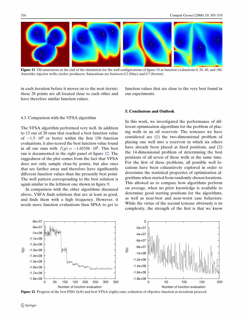
Figure 11 Oil saturations at the end of the simulation for the well configurations of figure 10 at function evaluations 0, 20, 40, and 100.Asterisks: injector wells; circles: producers. Saturations are between 0.2 (blue) and 0.7 (brown).

in each iteration before it moves on to the next iterate;these 28 points are all located close to each other andhave therefore similar function values.

4.3. Comparison with the VFSA algorithm

The VFSA algorithm performed very well. In additionto 13 out of 20 runs that reached a best function valueof −1.5 · 108 or better within the first 150 functionevaluations, it also scored the best function value foundin all our runs with f (p) = −1.65356 · 108. This bestrun is documented in the right panel of figure 12. Theraggedness of the plot comes from the fact that VFSAdoes not only sample close-by points, but also onesthat are farther away and therefore have significantlydifferent function values than the presently best point.The well pattern corresponding to the best solution isagain similar to the leftmost one shown in figure 9.

In comparison with the other algorithms discussedabove, VSFA finds solutions that are at least as good,and finds them with a high frequency. However, itneeds more function evaluations than SPSA to get to

function values that are close to the very best found inour experiments.

5. Conclusions and Outlook

In this work, we investigated the performance of dif-ferent optimization algorithms for the problem of plac-ing wells in an oil reservoir. The testcases we haveconsidered are (1) the two-dimensional problem ofplacing one well into a reservoir in which six othershave already been placed at fixed positions, and (2)the 14-dimensional problem of determining the bestpositions of all seven of these wells at the same time.For the first of these problems, all possible well lo-cations have been exhaustively explored in order todetermine the statistical properties of optimization al-gorithms when started from randomly chosen locations.This allowed us to compare how algorithms performon average, when no prior knowledge is available todetermine good starting positions for the algorithms,as well as near-best and near-worst case behaviors.While the virtue of the second testcase obviously is itscomplexity, the strength of the first is that we know

-1.8e+08

-1.6e+08

-1.4e+08

-1.2e+08

-1e+08

-8e+07

-6e+07

-4e+07

-2e+07

0

0 50 100 150 200

f(p)

Number of function evaluation

-1.8e+08

-1.7e+08

-1.6e+08

-1.5e+08

-1.4e+08

-1.3e+08

-1.2e+08

-1.1e+08

-1e+08

-9e+07

-8e+07

0 50 100 150 200 250 300 350

f(p)

Number of function evaluation

Figure 12 Progress of the best FDG (left) and best VFSA (right) runs: reduction of objective function as iterations proceed.

Comput Geosci (2006) 10: 303–319 317

the exact optimum and all other function values, whichallows us to do in-depth comparisons of the differentalgorithms.

On these testcases, we compared the simultane-ous perturbation stochastic approximation (SPSA), fi-nite difference gradient (FDG), very fast simulatedannealing (VFSA), and, for the first testcase, theNelder–Mead simplex and a genetic algorithm (GA)optimization methods. For the rather simple first test-case, both SPSA and VFSA reliably found very goodsolutions, and are significantly better than all the otheralgorithms; however, their different properties allowthem to be tailored to different situations: while SPSAwas very efficient in finding good solutions with a mini-mum of function evaluations, VFSA can be tweaked tofind the global optimum almost always, at the expenseof more function evaluations.

These observations also hold for the second, sig-nificantly more complex testcase. There, both SPSAand VFSA performed markedly better than the FDGalgorithm. Both algorithms found good solutions inmost of the runs that were started from different initialpositions. Again, SPSA was more efficient in findinggood positions for the seven wells in very few (around50) function evaluations, while VFSA obtained goodlocations more reliably but with more function eval-uations. FDG performed worse than the two otheralgorithms mainly because the high dimensionality ofthe problem requires too many function evaluations periteration to let FDG be competitive.

In this paper, we have only considered a limitednumber of methods; in particular, we have omit-ted Newton-type or other algorithms using second-derivative information. These may be subject of furtherstudies. However, we consider it uncertain whetherthey would be able provide superior performance: first,the objective functions considered here have manyminima, maxima, and saddlepoints (in particular it isnot convex), and second-order algorithms will only beable to perform well if curvature information is prop-erly accounted for. Second, the objective surfaces arevery rough in some parts of the parameter space (seefigures 3 and 4), particularly in the vicinity of theextrema, with roughness length scales on the sameorder of magnitude as the spacing of the integer latticeon which we optimize; it is therefore already hardto extract gradient information, as witnessed by theconsistently worse performance of the finite differencegradient method, and second derivative informationwill hardly contain much global information. Finally, inorder to be superior, such algorithms need to be contentwith very few iterations. For example, the NEWUOAalgorithm [36] for unconstrained optimization with-

out derivatives requires a recommended number of 5function evaluations per iteration for the single wellproblem, and 29 for the seven-well problem. On theother hand, our best algorithms only require on average30–50 and 200–250 function evaluations, respectively,which would mean that the Newton-type algorithmswould have to converge in 6–10 iterations; althoughpossible, it seems unlikely that algorithms can achieveor improve on this given the roughness of the solutionsurface.

While the results presented in this work are a goodindication as to which algorithms will perform well onmore complex problems, more experiments are neededin this direction. In particular, the fact that we have onlychosen the location of wells as decision variables is notsufficient to model the reality of oil reservoir manage-ment. For this, we would also have to allow for varyingpumping rates, different and more complex well types,and different completion times of wells. In addition,constraints need to be placed on the system, such asmaximal and minimal capacities of surface facilities,and the reservoir description must be more complexthan the relatively simple 2D case we chose here inorder to keep computing time within a range where dif-ferent algorithms can be easily compared. Also, it willbe interesting to investigate the effects of uncertaintyin the reservoir description on the performance of al-gorithms; for example, we expect that averaging overseveral possible realizations of a stochastic reservoirmodel may smooth out the objective function, whichwould probably aid the FDG algorithm more than theother methods. Research in these directions is presentlyunderway, and we will continue to investigate whichalgorithms are best suited for more complex and morerealistic descriptions of the oil well placement problem.

Acknowledgements The authors want to thank the NationalScience Foundation (NSF) for its support under the ITR grantEIA 0121523/EIA-0120934.

References

1. Arbogast, T., Wheeler, M.F., Yotov, I.: Mixed finite elementsfor elliptic problems with tensor coefficients as cell-centeredfinite differences. SIAM, J. Numer. Anal. 34(2), 828–852(1997)

2. Aziz, K., Settari, A.: Petroleum reservoir simulation. AppliedScience, London (1979)

3. Bangerth, W., Klie, H., Matossian, V., Parashar, M., Wheeler.M.F.: An autonomic reservoir framework for the stochas-tic optimization of well placement. Cluster Computing 8(4),255–269 (2005)

4. Becker, B.L., Song, X.: Field development planning usingsimulated annealing-optimal economic well scheduling and

318 Comput Geosci (2006) 10: 303–319

placement. In: SPE Annual Technical Conference and Exhi-bition, Dallas, Texas, SPE 30650, October 1995

5. Bittencourt, A.C., Horne, R.N.: Reservoir development anddesign optimization. In SPE Annual Technical Conferenceand Exhibition, San Antonio, Texas, SPE 38895, October1997

6. Carlson, M.: Practical reservoir simulation. PennWell Corpo-ration (2003)

7. Centilmen, A., Ertekin, T., Grader, A.S.: Applications ofneural networks in multiwell field development. In: SPEAnnual Technical Conference and Exhibition, Dallas, Texas,SPE 56433, October 1999

8. Chunduru, R.K., Sen, M., Stoffa, P.: Hybrid optimizationmethods for geophysical inversion. Geophysics 62, 1196–1207(1997)

9. Fanchi, J.R.: Principles of Applied Reservoir Simulation.Boston: Butterworth-Heinemann Gulf Professional Publish-ing, 2nd edn. (2001)

10. Gerencsér, L., Hill, S.D., Vágó, Z.: Optimization over dis-crete sets via SPSA. In Proceedings of the 38th Conference onDecision and Control, Phoenix, AZ, 1999, 1791–1795 (1999)

11. Gerencsér, L., Hill, S.D., Vágó, Z.: Discrete optimization viaSPSA. In: Proceedings of the Americal Control Conference,Arlington, VA, 2001, 1503–1504 (2001)

12. Goldberg, D.: Genetic Algorithms in Search, Optimization,and Machine Learning. Addison-Wesley (1989)

13. Guyaguler, B.: Optimization of well placement and as-sessment of uncertainty. PhD thesis, Stanford University,Department of Petroleum Engineering (2002)

14. Guyaguler, B., Horne, R.N.: Uncertainty assessment of wellplacement optimization. In: SPE Annual Technical Confer-ence and Exhibition, New Orleans, Louisiana, September,October 2001. SPE 71625

15. Helmig, R.: Multiphase Flow and Transport Processes in theSubsurface. Springer, Berlin (1997)

16. Houck, C., Joines, J.A., Kay, M.G.: A genetic algorithm forfunction optimization: A Matlab implementation. TechnicalReport TR 95-09, North Carolina State University (1995)

17. Hyne, N.: Nontechnical Guide to Petroleum Geology, Explo-ration, Drilling and Production. Pennwell Books, 2nd edn.(2001)

18. Ingber, L.: Very fast simulated reannealing. Math. Comput.Model. 12, 967–993 (1989)

19. Klie, H., Bangerth, W., Wheeler, M.F., Parashar, M.,Matossian, V.: Parallel well location optimization using sto-chastic algorithms on the grid computational framework. In:9th European Conference on the Mathematics of Oil Recov-ery, ECMOR, Cannes, France, EAGE August 30–September2, 2004

20. Lacroix, S., Vassilevski, Y., Wheeler, J., Wheeler, M.F.:Iterative solution methods for modelling multiphase flow inporous media fully implicitly. SIAM J. Sci. Comput. 25(3),905–926 (2003)

21. Lacroix, S., Vassilevski, Y., Wheeler, M.F.: Iterative solversof the Implicit Parallel Accurate Reservoir Simulator(IPARS). Numer. Linear Algebra Appl. 4, 537–549 (2001)

22. Lagarias, J.C., Reeds, J.A., Wright, M.H., Wright, P.E.: Con-vergence behavior of the Nelder–Mead simplex algorithm inlow dimensions. SIAM J. Optim. 9, 112–147 (1999)

23. Lu, Q.: A parallel multi-block/multi-physics approach formulti-phase flow in porous media. PhD thesis, University ofTexas at Austin, Austin, Texas (2000)

24. Lu, Q., Peszynska, M., Wheeler, M.F.: A parallel multi-blockblack-oil model in multi-model implementation. In: 2001SPE Reservoir Simulation Symposium, Houston, Texas, SPE66359 (2001)

25. Lu, Q., Peszynska, M., Wheeler, M.F.: A parallel multi-blockblack-oil model in multi-model implementation. SPE J. 7(3),278–287 SPE 79535 (2002)

26. Mattax, C.C., Dalton, R.L.: Reservoir simulation. In: SPEMonograph Series, volume 13, Richardson, Texas (1990)

27. Mitchell, M.: An Introduction to Genetic Algorithms. TheMIT Press (1996)

28. Nelder, J.A., Mead, R.: A simplex method for function mini-mization. Comput. J. 7, 308–313 (1965)

29. Nocedal, J., Wright, S.J.: Numerical Optimization. SpringerSeries in Operations Research. Springer, New York (1999)

30. Pan, Y., Horne, R.N.: Improved methods for multivariateoptimization of field development scheduling and well place-ment design. In: SPE Annual Technical Conference andExhibition, New Orleans, Louisiana, 27–30, SPE 49055September 1998

31. Parashar, M., Klie, H., Catalyurek, U., Kurc, T., Bangerth,W., Matossian, V., Saltz, J., Wheeler, M.F.: Application ofgrid-enabled technologies for solving optimization problemsin data-driven reservoir studies. Future Gener. Comput. Syst.21(1), 19–26 (2005)

32. Parashar, M., Wheeler, J.A., Pope, G., Wang, K., Wang, P.:A new generation EOS compositional reservoir simulator.Part II: Framework and multiprocessing. In: Fourteenth SPESymposium on Reservoir Simulation, Dallas, Texas, 31–38.Society of Petroleum Engineers June 1997

33. Parashar, M., Yotov, I.: An environment for parallel multi-block, multi-resolution reservoir simulations. In: Proceedingsof the 11th International Conference on Parallel and Distrib-uted Computing and Systems (PDCS 98), 230–235, Chicago,IL, International Society for Computers and their Applica-tions (ISCA) Sep. 1998

34. Pardalos, P.M., Resende, M.G.C. eds.: Handbook of AppliedOptimization, pp. 808–813. Oxford University Press (2002)

35. Peszynska, M., Lu, Q., Wheeler, M.F.: Multiphysics couplingof codes. In: L.R. Bentley, J.F. Sykes, C.A. Brebbia, W.G.Gray, G.F. Pinder, eds., Computational Methods in WaterResources, 175–182. A. A. Balkema (2000)

36. Powell, M.J.D.: The NEWUOA software for unconstrainedoptimization without derivatives. Technical Report DAMTP2004/NA08, University of Cambridge, England (2004)

37. Rian, D.T., Hage, A.: Automatic optimization of well loca-tions in a north sea fractured chalk reservoir using a fronttracking reservoir simulator. In: SPE International Petro-leum & Exhibition of Mexico, Veracruz, Mexico, SPE 28716,October 2001

38. Russell, T.F., Wheeler, M.F.: Finite element and finite dif-ference methods for continuous flows in porous media. In:R.E. Ewing, eds., The Mathematics of Reservoir Simulation,pp. 35–106. SIAM, Philadelphia (1983)

39. Sen, M., Stoffa, P.: Global Optimization Methods in Geo-physical Inversion. Elsevier (1995)

40. Spall, J.C.: Multivariate stochastic approximation using asimultaneous perturbation gradient approximation. IEEETrans. Autom. Control. 37, 332–341 (1992)

41. Spall, J.C.: Adaptive stochastic approximation by the simulta-neous perturbation method. IEEE Trans. Autom. Contr. 45,1839–853 (2000)

42. J.C. Spall. Introduction to Stochastic Search and Optimiza-tion: Estimation, Simulation and Control. Wiley, New Jersey(2003)

43. Wang, P., Yotov, I., Wheeler, M.F., Arbogast, T., Dawson,C.N., Parashar, M., Sepehrnoori, K.: A new generation EOScompositional reservoir simulator. Part I: Formulation anddiscretization. In: Fourteenth SPE Symposium on Reservoir

Comput Geosci (2006) 10: 303–319 319

Simulation, Dallas, Texas, pp. 55–64. Society of PetroleumEngineers, June 1997

44. Wheeler, M.F.: Advanced techniques and algorithmsfor reservoir simulation, II: The multiblock approachin the integrated parallel accurate reservoir simulator(IPARS). In: J. Chadam, A. Cunningham, R.E. Ewing,P. Ortoleva, M.F. Wheeler, eds., IMA Volumes inMathematics and its Applications, Volume 131: ResourceRecovery, Confinement, and Remediation of EnvironmentalHazards. Springer (2002)

45. Wheeler, M.F., Wheeler, J.A., Peszynska, M.: A distributedcomputing portal for coupling multi-physics and multipledomains in porous media. In: L.R. Bentley, J.F. Sykes,C.A. Brebbia, W.G. Gray, G.F. Pinder, eds., ComputationalMethods in Water Resources, 167–174. A. A. Balkema (2000)

46. Yeten, B.: Optimum deployment of nonconventional wells.PhD thesis, Stanford University, Department of PetroleumEngineering (2003)

47. Yeten, B., Durlofsky, L.J., Aziz, K.: Optimization of non-conventional well type, location, and trajectory. SPE J. 8(3),200–210 SPE 86880 (2003)

48. Yotov, I.: Mortar mixed finite element methods on irregu-lar multiblock domains. In: J. Wang, M.B. Allen, B. Chen,T. Mathew, eds., Iterative Methods in Scientific Computa-tion, IMACS series Comp. Appl. Math., vol. 4, 239–244.IMACS, (1998)

49. Zhang, F., Reynolds, A.: Optimization algorithms for auto-matic history matching of production data. In: 8th EuropeanConference on the Mathematics of Oil Recovery, ECMOR,Freiberg, Germany, EAGE, September 2002