ON NEURO-FUZZY APPLICATIONS FOR AUTOMATIC

CONTROL, SUPERVISION, AND FAULT DIAGNOSIS FOR

WATER TREATMENT PLANT

KASUMA BIN ARIFFIN

A project submitted in partial fulfillment of the

requirements for the award of the degree of

Master of Engineering (Electrical – Mechatronics And Automatic Control)

Faculty of Electrical Engineering

Universiti Teknologi Malaysia

MAY 2007

iii

To my beloved mother and father

iv

ACKNOWLEDGEMENT

I would like to express my sincere appreciation and gratitude to my thesis

supervisor, Dr. Mohd Fauzi Bin Othman, for his invaluable ideas, support, critics

and encouragement guidance since the first beginning of this project. He has far

exceeded the expectations of a great supervision and provided means for the

establishment of the grounds of a good friendship.

At last, but not least, I am extremely grateful to my parents Ariffin Bin Alias

and Mariam Binti Saibi. I am grateful to all my family members. Without their

unlimited dedication, support and love throughout so many years, I would never

have got this far. My sincere appreciation also extends to all my colleagues and

others who have provided assistance at various occasions. Their views and tips are

useful indeed. Unfortunately, it is not possible to list all of them in this limited

space.

v

ABSTRACT

Water treatment includes many complex phenomena, such as coagulation

and flocculation. These reactions are hard or even impossible to control satisfyingly

by conventional methods. Biological water treatment systems are difficult to model

because their performance is complex and varies significantly with different reactor

configurations, influent characteristics, and operational conditions. Neuro-fuzzy

ANFIS method, which is chosen as the method in this case, is a new intelligent

method in this line of process industry. Although intelligent tools such as neural

network, fuzzy logic and neuro-fuzzy methods have been applied in real time water

treatment plant for some time, problems of monitoring water treatment processes

and assessing uncertainty for the coagulant dosing rate represent a major challenged

that need to be investigated. In this research, statistical methods are used to analyze

nonstationary time series water treatment process where they are accrued from a

neuro-fuzzy ANFIS model. The proposed scheme is evaluated in computer

simulation studies using real process data before application to the real plant.

vi

ABSTRAK

Pembersihan air melibatkan banyak fenomena kompleks seperti pembekuan

dan proses penapisan Reaksi seperti ini adalah sukar dan amat mustahil sekali untuk

dikawal dengan jayanya melalui cara yang biasa dilakukan. Sistem biologikal

pembersihan air adalah sukar untuk dipamerkan kerana prestasinya yang begitu

kompleks dan sacara signifikan berbeza dengan tatarajah tindakan, pengaruh sifat

dan keadaan operasi. Penggunaan Neuro-fuzzy ANFIS, di mana ia merupakan

kaedah yang telah dipilih untuk pemyelidikan ini, adalah kaedah baru dan bijak

yang selari dengan proses industri kini. Walaupun kaedah perkakasan yang bijak

seperti rangkaian neural, logic fuzzy, dan neuro-fuzzy telah diaplikasikan dalam

masa nyata loji perbersihan air untuk beberapa waktu ini, masalah memantau proses

pembersihan air dan menilai ketidakpastian untuk kadar sukatan kepekatan

memperlihatkan cabaran utama yang perlu dikaji dengan lebih lanjut. Dalam

penyelidikan ini ,kaedah statistik digunakan untuk menganalisa siri masa yang

bergerak dalam proses pembersihan air dimana ia diakrukan dari neuro-fuzzy

ANFIS. Cadangan yang telah dipilih adalah dengan membina penilaian simulasi

komputer dengan memproses data masa nyata sebelum mengaplikasikannya kepada

keadaan yang sebenar.

vii

TABLE OF CONTENTS

CHAPTER TITLE PAGE

DECLARATION ii

DEDICATION iii

ACKNOWLEDGEMENTS iv

ABSTRACT v

ABSTRAK vi

TABLE OF CONTENTS vii

LIST OF TABLES x

LIST OF FIGURES xi

LIST OF ABBREVIATIONS xv

LIST OF APPENDICES xvi

1 INTRODUCTION 1

1.1 An Overview of Water Treatment 2

1.2 Chemical Plant Overview 3

1.2.1 Water Treatment Chemicals 3

1.2.2 Lime Operation 3

1.2.2.1 Lime Plant Operation in Manual Mode 4

1.2.3 Fluoride Operation 6

1.2.3.1 Fluoride Plant Operation in Manual Mode 7

1.2.4 Chlorine Operation 9

1.2.4.1 Chlorine Plant Operation in Manual Mode 10

1.3 Neuro-Fuzzy and Soft Computing 12

viii

1.3.1 Neural Networks 13

1.3.2 Fuzzy Logic 15

1.3.3 Soft Computing 18

2 RESEARCH OBJECTIVES 19

2.1 Need for Research 19

2.2 Research Objectives 20

3 BACKGROUND AND LITERATURE REVIEW 21

3.1 Fuzzy Logic 22

3.1.1 Fuzzy Sets 22

3.1.2 Membership Functions 24

3.1.3 Fuzzy If-Then Rules 24

3.1.4 Fuzzy Reasoning 26

3.1.5 Fuzzy Inference Systems 27

3.1.6 Fuzzy Modeling 29

3.2 Neural Networks 30

3.2.1 Supervised Learning 30

3.2.2 Unsupervised Learning 32

3.3 Neuro-Fuzzy Systems 35

3.3.1 General Neuro-Fuzzy Architecture 36

3.3.2 ANFIS Architecture 37

3.3.3 Hybrid Learning 40

4 METHODOLOGY AND RESULT 42

4.1 Fuzzy Inference Systems 42

4.1.1 Fuzzy Sets 43

4.1.2 Using Matlab Fuzzy Toolbox GUI 44

ix

4.1.3 Conclusion 60

4.2 ANFIS (Adaptive Neuro-Fuzzy Inference System) 61

4.2.1 The ANFIS Editor GUI 62

4.2.2 MATLAB Final Management 64

4.2.3 Data Preparation 65

4.2.4 Structure Identification 65

4.2.5 Result 70

4.2.6 Conclusion 77

5 CONCLUSIONS AND FUTURE RESEARCH

RECOMMENDATIONS 78

5.1 Summary of Research 78

5.2 Recommendations for Future Research 80

REFERENCES 82

Appendices A - B 84-88

x

LIST OF TABLES

TABLE NO. TITLE PAGE

1.1 List of chemicals with estimated dosages 3

xi

LIST OF FIGURES

FIGURE NO. TITLE PAGE

1.1 Schematic diagram of water treatment process 2

1.2 Lime-Plant Dosing 4

1.3 VSD key SF101 5

1.4 Fluoride Plant 7

1.5 Post Chlorination Plant 10

3.1 Cores, supports, boundaries, crossover points

of membership function 23

3.2 Node j of a backpropagation MLP 31

3.3 A backpropagation multilayer perceptron 31

3.4 Reducing neighborhoods around node x 34

3.5 General neuro-fuzzy architecture 37

3.6 A two-input first-order Sugeno fuzzy model 38

xii

3.7 Equivalent ANFIS architecture 39

4.1 Membership functions may assume different shapes

like bell-shaped, triangular, trapezoidal and singleton 44

4.2 Naming the input variable in GUI 45

4.3 Set the range in GUI 46

4.4 Three triangular membership functions have been chosen

for flow input 47

4.5 Fuzzy system with two inputs; Flow and Turbidity 48

4.6 Two triangular membership functions have been chosen

for turbidity input 49

4.7 Fuzzy system with two inputs, Flow and Turbidity and

three outputs, pH, Fluoride, Chlorine 50

4.8 Three triangular membership functions have been

chosen for pH output 51

4.9 Three triangular membership functions have been chosen

for Fluoride output 52

4.10 Three triangular membership functions have been chosen

for Chlorine output 53

4.11 Rule Editor display 54

4.12 Result of fuzzy reasoning 55

4.13 Changing the input value result in different output values 56

xiii

4.14 Changing the input value result in different pH output

values 57

4.15 Changing the input value result in different fluoride output

values 58

4.16 Changing the input value result in different chlorine output

values 59

4.17 ANFIS Editor 63

4.18 Load data to ANFIS Editor 66

4.19 Generate FIS 67

4.20 Training data 68

4.21 FIS test 69

4.22 Output membership of neuro-fuzzy model generated 70

4.23 The output neuro-fuzzy model rules generated 71

4.24 The output neuro-fuzzy model rules generated in Rules

Editor 72

4.25 The generated Sugeno Model Structure 73

4.26 The generated Sugeno Model from Surface viewer 74

4.27 The command to test the output of generated Sugeno

model 75

xiv

4.28 Output generated by Sugeno model 76

xv

LIST OF ABBREVIATIONS

ANFIS - Adaptive Neuro Fuzzy Inference Systems

BP - Backpropagation

C - Concentration solution

GDM - Gradient Descent Method

GDR - Generalized Delta Rule

MCC - Motor Control Center

MLD - Minimum lumen diameter

MLP - multilayer perceptrons

LSE - least-square estimator

PE - processing element

ppm @ mg/L - Dosage rate

SC - Soft Computing

S.G - Specific gravity of solution

VSD - Value Sensitive Design

xvi

LIST OF APPENDICES

APPENDIX TITLE PAGE

A Basic concepts and terminology of membership

functions 84

B Four commonly used membership functions 86

CHAPTER 1

INTRODUCTION

The water industry is seeking ways to produce high quality water at reduced

cost. The operation of water treatment plants is significantly different from most

manufacturing industrial operations because raw water sources are often subject to

natural perturbations like flood and drought, both of which significantly affect the

characteristics of the abstracted water. Whilst it is possible to measure some of

these variables with commercially available instrumentation, the general experience

is that the instruments often lack the required reliability, accuracy and robustness.

Consequently, early applications of automatic control in the water industry were

often compromised. More recently, improved sensor technology has enabled the

successful regulation of variables such as pH and chlorine residual. Without a

precise knowledge of the characteristics of the material to be removed, most

chemical dosage requirements for primary water treatment are determined from

laboratory measurements (jar tests) which are conducted (usually) at regular time

intervals. Excessive overdosing is not only expensive but may lead to increased

public health concerns. This paper will begin with a brief explanation of water

treatment plant operation.

2

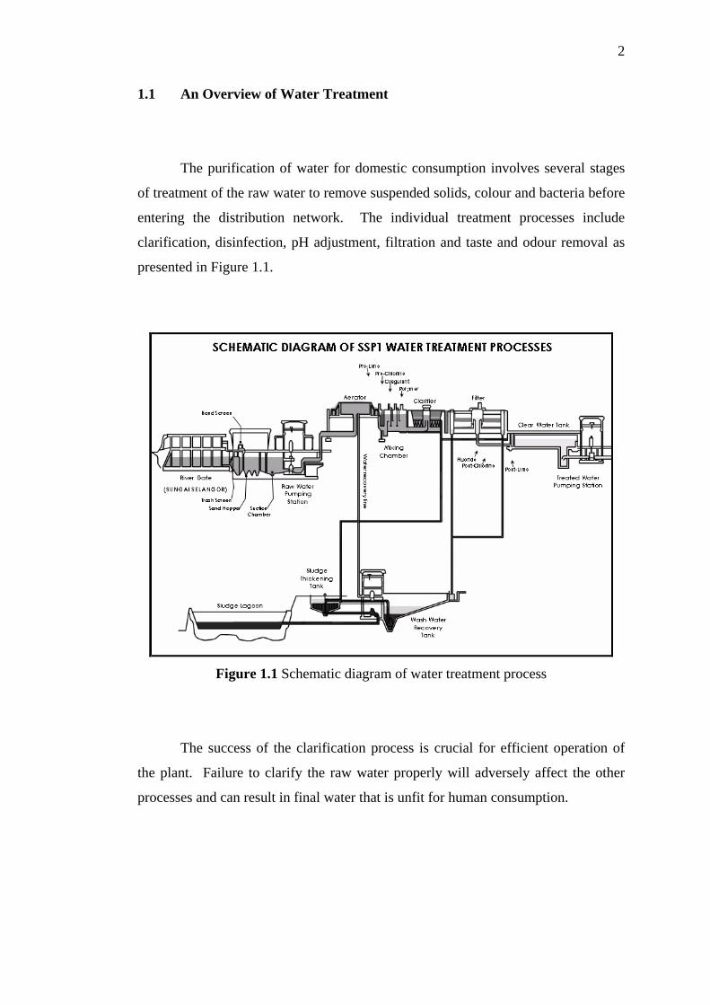
1.1 An Overview of Water Treatment

The purification of water for domestic consumption involves several stages

of treatment of the raw water to remove suspended solids, colour and bacteria before

entering the distribution network. The individual treatment processes include

clarification, disinfection, pH adjustment, filtration and taste and odour removal as

presented in Figure 1.1.

Figure 1.1 Schematic diagram of water treatment process

The success of the clarification process is crucial for efficient operation of

the plant. Failure to clarify the raw water properly will adversely affect the other

processes and can result in final water that is unfit for human consumption.

3

1.2 Chemical Plant Overview

The chemical plant is designed for handling of aluminium sulphate, hydrated

lime, polyelectrolyte, chorine, sodium silicon fluoride and ammonia.

1.2.1 Water Treatment Chemicals

The following is a list of chemicals with estimated dosages which may be

necessary to meet the final treated quality specified.

Table 1.1: List of chemicals with estimated dosages

Chemical Function Estimated Dosage(mg/l)

For filtered water Min Average Max

Chlorine Disinfection 0.5 3 5

Hydrated Lime (as 90% Ca(OH)2 pH correction 2 6 10

Sodium Silicon Fluoride (as 1%F) Dental protection 0.7 0.8 0.9

1.2.2 Lime Operation

The hydrated lime chemical as delivered should contain a calcium hydroxide

Ca(OH)2 content of not less then 90%. The chemical is to be delivered by bulk air

pressure road tankers, having a capacity of up to 20 tons. It should always be

ensured therefore that the available capacity in a silo to receive chemical is in

4

multiples of 20 tons leaving ample room to spare as an allowance for initial aeration.

It is recommended that the silo available capacity should not be less than 27 tons for

a 20 tons bulk road tanker delivery.

Figure 1.2 Lime-Plant Dosing

1.2.2.1 Lime Plant Operation in Manual Mode

Introduction

Lime Plant must be operated in manually if the flow meter for raw

water/filtered water not functioning. Due to this, VSD value must be set manually

based on water flow.

Equipment

(i) Lime MCC panel

(ii) VSD key

(iii) VSD panel

5

Procedure

(i) Go to the Lime Plant.

(ii) Check the Lime MCC panel.

(iii) Make sure the power supply is ON.

(iv) After that, go to VSD panel.

(v) Select either option 1 or 2.

(vi) By using the VSD key SF101, turn the VSD key to fix position.

(vii) ( Please refer to figure below)

Figure 1.3 VSD key SF101

(viii) Then, use the black button beside the VSD panel to set the VSD

recording to value requires.

(ix) Write down the VSD reading in FRM/CP/01 form.

(x) VSD value will change according to total flow reading.

Formula of Lime Dosage

Liter/day = Flow(MLD)*Dosage rate / C * S.G

Liter/hour= Flow(MLD)*Dosage rate /24*C*S.G

Liter /min = Flow(MLD*Dosage rate/24*60*C*S.G

C = Concentration solution

S.G = Specific gravity of solution

fix

off

variable

6

Dosage rate = ppm @ mg/L

Example 1

Total usage of Lime in a day is 5 ton and the total water flow is 600000m3. What is

the average dosage rate ppm of lime that has been used?

Solution:

Dosing rate = Flow * Dosage rate; kg/day = Flow (MLD) * ppm;

Flow=600000m3.kg/day = 5 ton = 5000kg

Kg/day=flow*ppm

Ppm=5000/600=8.33

1.2.3 Fluoride Operation

The sodium silicofluoride chemical is to be supplied in 25kg bags’ charging

of the dry feeder storage hopper is to be carried out only during the day shift. It is

intended that the dosing rate should not exceed 1.5mg/l, the average dose being 1.3

mg/l. The preparation system is designed so that an inflow of 2.06 litres/sec enters

the dissolving tank. The solution strength will be maintained according to the plant

flow but the dosing rate is under manual control.

7

Figure 1.4 Fluoride Plant

1.2.3.1 Fluoride Plant Operation in Manual Mode

Introduction

Fluoride plant operation is based on VSD value that is manually operated.

The VSD value required is proportional with filtered water flow

Equipment

VSD machine

Procedure

(i) Go to fluoride MCC panel.

(ii) Make sure the power supply is ON.

(iii) Then go to VSD machine.

(iv) Press the green button to run the VSD machine.

8

(v) Press “^” button to increase the VSD value to value required.

(vi) Press “v” button to decrease the VSD value to value required.

(vii) Check the VSD reading displayed on the screen.

(viii) Write down the VSD reading in FRM/CP/01 form.

Formula of Fluoride Dosage

Dosing rate (kg/day) = Flow(MLD)*Dosage rate(mg/L)

Dosing rate (kg/hr) = Flow(MLD)*Dosage rate(mg/L)

Dosing rate (kg/min) = Flow(MLD)*Dosage rate(mg/L)/ 24*60

Dosing rate (g/min) = Flow(MLD)*Dosage rate(mg/L)*1000/24*60

Example 1

Fluoride that flow from the feeder is 200g/min. Raw water flow reading is 400MLD.

Calculate the fluoride dosage rate.

Solution:

Flow=400; g/min=200; Dosage rate = x

From formula no. 4

200 = (400*x*1000)/24*60

x = 200*24*60/400*1000 = 0.72 mg/L@ppm

Example 2

Total of fluoride used in a day is 800kg. Total raw water flow is 600000m3. What is

the average of dosage rate fluoride dosage required?

Solution:

9

Flow=600000m3/day=600000/1000=600MLD; kg/day=800; dosage rate =x

From formula no.1

800 = 600*x

x = 800/600

x = 1.3 mg/L@ ppm

1.2.4 Chlorine Operation

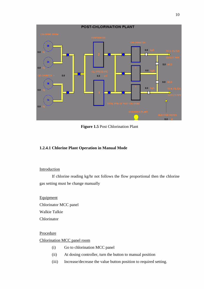
Chlorine is to be supplied in drums containing 915kg of liquid chlorine. The

duty drums supply liquid chlorine to evaporators that converts the liquid to a

chlorine gas which is the conveyed to gas control chlorination units. The dosing rate

is manually set and is maintained proportional to flow as mentioned previously for

raw water the dose rate to the filtered water, is also under manual control for

chlorine residual.

10

Figure 1.5 Post Chlorination Plant

1.2.4.1 Chlorine Plant Operation in Manual Mode

Introduction

If chlorine reading kg/hr not follows the flow proportional then the chlorine

gas setting must be change manually

Equipment

Chlorinator MCC panel

Walkie Talkie

Chlorinator

Procedure

Chlorination MCC panel room

(i) Go to chlorination MCC panel

(ii) At dosing controller, turn the button to manual position

(iii) Increase/decrease the value button position to required setting.

11

(iv) Then watch the dose rate kg/hr reading at active chlorinator panel.

Chlorinator Room

(i) Go to chlorinator room

(ii) Check the chlorine gas kg/hr reading at chlorinator on duty.

(iii) Jot down the chlorinator reading in FRM/CP/01 form.

Formula of Chlorine Dosage

Dosing rate = Flow (MLD) * Dosage rate (kg/day)

Dosing rate = Flow (MLD)* Dosage rate/24 (kg/hr)

Chlorine Dosing rate = Chlorine Demand + chlorine residual

(mg/L) (mg/L) (mg/L)

(i) Dosage rate in ppm or Mg/L

(ii) Flow must be in MLD form.

Example 1

Flow given is 600MLD.While required dosage rate require is 3ppm. Find dosing rate

needed in kg/hr.

Solution:

Dosing rate (kg/hr) = Flow * ppm/24

Flow = 600; Dosage rate = 3

Dosing rate = (600*3)/24 = 75kg/hr

Example 2

Flow given is 500MLD. Total dosing used was 60kg/hr. What is the chlorine dosage

rate?

12

Solution:

Flow = 500; Dosing rate = 60

From formula

60 = 500*x /24

x = 60*24/500 = 2.88

1.3 Neuro-Fuzzy and Soft Computing

Analysis of real world problems requires intelligent systems. Soft

Computing (SC) is an innovative approach to constructing computationally

intelligent systems (Jang, Sun and Mizutani, 1997). These intelligent systems,

which combine knowledge, techniques, and methodologies from various sources, are

supposed to possess human-like expertise within a specific domain, adapt

themselves and learn to do better in changing environments, and explain how they

make decisions or take actions. In confronting complex real-world computing

problems, it is frequently advantageous to use several computing techniques

synergistically rather than exclusively, resulting in the construction of

complementary hybrid intelligent systems. One of the most successful of this kind

of intelligent systems design is neuro-fuzzy computing: neural networks recognize

patterns and learn from examples; fuzzy inference systems incorporate human

knowledge and perform inferencing. In the following section, a brief description of

these emerging fields is provided.

13

1.3.1 Neural Networks

A neural network is a parallel, distributed information processing structure

consisting of processing elements (which can possess a local memory and

can carry out localized information processing operations) interconnected via

unidirectional signal channels called connections. Each processing element

has a single output connection that branches (“fans out”) into as many

collateral connections as desired; each carries the same signal – the

processing element output signal. The processing element output signal can

be of any mathematical type desired. The information processing that goes

on within each processing element can be defined arbitrarily with the

restriction that it must be completely local; that is, it must depend only on the

current values of the input signal arriving at the processing element’s local

memory.

(Hecht-Nielsen, 1990)

Clearly, neural networks are models based on the working mechanism of the

human brain; they are composed of individual interconnected processing elements

(PEs), which are analogous to neurons in the brain and utilize a distributed

processing approach to computation.

More specifically, anything that can be represented as a number might be fed

into a neural network. Each PE sends/receives data to/from other PEs. For each

individual PE in standard model, input data (X0…X

n) are multiplied by the weights

(W0…W

n) associated with the connection to the PE. Each PE applies a nonlinear

activation function to its sum of weighted input signals to determine its output

signal. The output from a given PE is multiplied by another separate weight and fed

into the next processing element. If the processing element is in the output layer,

14

then the output from the processing element is not multiplied by a weight and

instead is an output of the network itself.

The origin of the neural network field began in the 1940s with the work of

McCulloch and Pitts (1943), who showed that networks of artificial neurons could,

in principle, compute any arithmetic or logical function. They also showed that any

arbitrary logical function could be configured by a neural network of interconnected

digital neurons, which introduced the idea of the step threshold used in many neural

network models. The first practical application of artificial neural networks was

presented by Rosenblatt in the late 1950s. In his book published in 1962, Principles

of Neurodynamics, he introduced a learning algorithm by which the weights can be

changed, and he demonstrated the ability to perform pattern recognition in a

perceptron network. At about the same time, Widrow and Hoff introduced a new

learning algorithm in 1960 and used it to train adaptive linear neural networks,

which were similar in structure and capability to Rosenblatt’s perceptron.

Unfortunately, both Rosenblatt’s and Widrow’s networks suffered from the

same inherent limitations as pointed out in the book Perceptrons by Minsky and

Papert, published in 1969. They showed that single-layer systems were limited and

expressed pessimism over multilayer systems. Interest in neural networks dwindled

from late 1960s to early 1980s.

The breakthrough of neural network came in the 1980s when the most

influential method of training a multilayer neural network, known as the

backpropagation (BP) algorithm was developed by Parker (1982) and Rumelhart &

McClelland (1986). About the same time, new types of neural net with dynamic

behavior, such as Hopfield neural net (Hopfield, 1982; 1984) and the Kohonen self-

15

organizing neural net (Kohonen, 1982; 1984), were introduced. These new

developments reinvigorated the field of neural networks.

Neural networks are capable of solving a wide range of problems by

“learning”, “generalizing” and “abstracting”. They can modify their behavior in

response to their environment and once trained, the network’s response can be

tolerant to minor variations to its input. As a matter of fact, neural networks have

been widely used in a broad range of areas such as image processing, signal

processing, pattern recognition, speech recognition, industrial control, aerospace,

manufacturing, medicine, business, finance, and even literature. The success in

application of neural networks is mostly because of their applicability to complex

nonlinear systems and multivariable systems.

1.3.2 Fuzzy Logic

We need a radically different kind of mathematics, the mathematics of fuzzy

or cloudy quantities which are not described in terms of probability

distributions. Indeed, the need for such mathematics is becoming

increasingly apparent… for in most practical cases the a priori data as well as

the criteria by which the performance of a man-made system is judged are far

from being precisely specified or having accurately known probability

distributions.

(Zadeh, 1961)

16

Fuzzy set theory, originally introduced by Lotfi Zadeh in the 1960’s,

resembles human reasoning in its use of approximate information and uncertainty to

generate decisions. It was specifically designed to mathematically represent

uncertainty and vagueness and provide formalized tools for dealing with the

imprecision intrinsic to many problems.

Zadeh’s idea of membership grade is the backbone of fuzzy set theory. In

1965, the publication of his seminal paper on fuzzy sets declared the birth of fuzzy

logic technology. Narrowly speaking, fuzzy logic refers to a logical system that

generalizes classical two-valued logic for reasoning under uncertainty. Broadly

speaking, fuzzy logic refers to all of the theories and technologies that employ fuzzy

sets, which are classes with unsharp boundaries (Yen and Langari, 1999).

Even though the concept of fuzzy sets encountered sharp criticism from the

academic community at the beginning, many researchers around the world still kept

stepping into this field. During the first decade (1965-1975), Zadeh continued to

broaden the foundation of fuzzy set theory. He introduced fuzzy multistage

decision-making, fuzzy similarity relations, fuzzy restrictions, and linguistic hedges.

Mamdani and Assilian (1975) developed the first fuzzy logic controller to control a

steam generator in 1974. In 1976, the first industrial application of fuzzy logic was

developed by Blue Circle Cement and SIRA in Denmark. Another successful

application is a fuzzy logic based automatic train operation control system in Sendai

city’s subway system developed by Yasunobu and his colleagues at Hitachi in 1987.

Researchers in Japan made many important contributions to the theory as well as to

the applications. In 1980s, Takagi and Sugeno developed the first approach for

constructing fuzzy rules based on the training data. This important work did not

gain much immediate attention, but it built the foundation for fuzzy model

identification.

17

The fuzzy boom in Japan triggered a broad interest in the world. Fuzzy

logic is now being widely used in aerospace, defense, automobile, consumer

products, industry, manufacturing, business and finance. The main reason for its

popularity is that it utilizes concepts and knowledge that do not have well-defined,

sharp boundaries; therefore, it can alleviate the difficulties encountered by

conventional mathematical tools in developing and analyzing complex systems.

Fuzzy set theory implements classes or groupings of data with boundaries

that are not sharply defined. Any methodology or theory implementing “crisp”

definitions such as classical set theory, arithmetic, and programming, may be

“fuzzified” by generalizing the concept of a crisp set to a fuzzy set with blurred

boundaries. The benefit of extending crisp theory and analysis methods to fuzzy

techniques is the strength in solving real world problems, which inevitably entail

some degree of imprecision and noise in the variables and parameters measured and

processed. Fuzzy logic comprises of fuzzy sets and fuzzy rules which combine

numerical and linguistic data. Linguistic variables are a critical aspect of some

fuzzy logic application, where general terms such as “large”, “medium”, and “small”

could be used to capture a range of numerical values. Such terms are not precise and

cannot be represented in normal set theory. While similar to conventional

quantization, fuzzy logic allows these stratified sets to overlap and allows members

to be partial members as well as the normal multi-set membership.

Since fuzzy logic can handle approximate information in a systematic way, it

is ideal for dealing with nonlinear systems and for modeling complex systems where

no exact model exists or systems where ambiguity or vagueness is common.

18

1.3.3 Soft Computing

Soft computing is an emerging approach to computing which parallels the

remarkable ability of the human mind to reason and learn in an environment

of uncertainty and imprecision.

(Zadeh, 1992)

Soft computing consists of several computing paradigms, including neural

networks, fuzzy set theory, approximate reasoning, and derivative-free optimization

methods such as genetic algorithms and simulated annealing. As for the major part

of these constituent methodologies, neural network has the strength of learning and

adaptation, fuzzy logic has the strength of knowledge representation via fuzzy if-

then rules, and genetic algorithm is suitable for systematic random search.

Although fuzzy logic and neural network emphasize different strengths,

these two innovative modeling approaches share some common characteristics: they

assume parallel operations; they are well known for their fault tolerance capabilities;

and they have the ability of model-free learning, i.e. the ability to construct models

using only target system sample data. Despite these similarities, they stem from

very different origins. Primarily, fuzzy logic modeling is based on fuzzy sets and

fuzzy if-then rules proposed by Zadeh, which are closely related to psychology and

cognitive sciences, while neural network modeling is based on artificial neural

networks which are motivated by biological neural systems (Jang, 1992). Because

of their very origins, the respective philosophies and methodologies underlying their

problem solving approaches are quite different and, in general, complementary.

Therefore, they can be integrated to generate hybrid models that can take advantage

of the strong points of both.