Embed Size (px)
Citation preview
On Modeling Magnetic Fields on a Sphere with Dipoles and QuadrupolesA <*Nfc/ JL
GEOLOGICAL SURVEY PROFESSIONAL PAPER 1118
On Modeling Magnetic Fields on a Sphere with Dipoles and QuadrupolesBy DAVID G. KNAPP
GEOLOGICAL SURVEY PROFESSIONAL PAPER 1118
A study of the global geomagnetic field with special emphasis on quadrupoles
UNITED STATES GOVERNMENT PRINTING OFFICE, WASHINGTON: 1980
UNITED STATES DEPARTMENT OF THE INTERIOR
CECIL D. ANDRUS, Secretary
GEOLOGICAL SURVEY
H. William Menard, Director
Library of Congress Cataloging in Publication DataKnapp, David Goodwin, 1907-On modeling magnetic fields on a sphere with dipoles and quadrupoles.(Geological Survey Professional Paper 1118)Bibliography: p. 351. Magnetism, Terrestrial Mathematical models. 2. Quadrupoles. I. Title. II. Series: United States
Geological Survey Professional Paper 1118. QC827.K58 538'.?'ol84 79-4046
For sale by the Superintendent of Documents, U.S. Government Printing OfficeWashington, D.C. 20402
Stock Number 024-001-03262-7
CONTENTS
Page/VOStrHCt ™™-™™™™"™-™™™"™«™™-«—"—————————————— j_
Introduction——————————-—--——-———........—..——....... iCharacteristics of the field of a dipole —————————————— 1Multipoles ——————————-—--——--—-——--——-——...._. 2The general quadrupole ——————-———._....................—.— 2
Some characteristics of quadrupole fields -————————- 4Character of lines of force ———————————————— 6Interconversion of quadrupoles —————————————— $
Relations with spherical harmonic analysis —————————— 9Quadrupole secular change and its conservative aspect — 12The eccentric dipole ——————————————————— 13Fertile and sterile parts of the quadrupole ———————— 13
Relations with spherical harmonic analysis—ContinuedOther remarks concerning eccentric dipoles ————
Application to extant models -—————————-——-E ccentric-dipole behavior ———————————————• Results of calculations --—--—------——-——-—-Additional results ————————————————
Hypothesis on the character of the quadrupole —————-Some further implications of the quadrupole constraint — Some qualitative remarks on octupoles ——————.—...Summary and conclusions -----———————————-—~Selected references ——————————————————————
Page
14142021262729343535
ILLUSTRATIONS
PageFIGURES 1-4. Sketches of:
1. Linear quadrupoles -—--————————-———---——————--———————————...——————— 22. Three conceptions of the rhombic quadrupole ————-——--———————---—————————-----——— 33. Linear quadrupoles on a sphere directed toward P0 and Pj ——————--—-—-——-——-—---———--— 34. Attitude of quadrupole shown in figures 5-7 -----——————————————————-———-——-————-— 6
5-7. Graphs of normal-quadrupole field on the sphere showing:5. Potential, vertical intensity, and inclination ————————————————————————......————— 76. Magnetic meridians, declination, and horizontal and total intensity ——————————————————-—-— 77. North and east components ———--—--------———--—--—-_-———————————-———————————————— 7
8-11. Sketches of:8. Dipole field line -.-----.-------------------------------------.---------.-----.----------------------------------------------------------------------------———- 89. Linear-quadrupole field line ---------—————-———————-—-——————————--——--—-----——- 8
10. Normal-quadrupole field line-----------------------------—--—--—-———-—-—-----————————————— 811. Relations of cardinal axes to primitive lines and identification of angular parameters ————---————— 11
12-17. Graphs of drift of the geomagnetic quadrupole:12. Primary axis since 1550 —————————————————————————————————————————————— 1513. Primary axis since 1930 ---------------------------------———-——-——---————————-———...——— jg1 A. T?pH (*ai*Hinfi 1 avic GITI/"»O 1 ^^O -.—..—_.._-.___— _ _..______ _ _....._..—————————_—.._———..—————.——— 1 7J-^T. J.1/CU \^CLL U111CIJ. CUVlO OlllVsC J.tltlV/ ————————— j_ i
15. Red cardinal axis since 1930 ————————————————————————————————————————————— 17J.O. XJlUc CHiQlrlHI HX1S 31HC6 J.O«5vJ ———————---------.————-—---——----————-———————————--—--—————————————————---»«-•••-•--•-- J.o
1 7 Rind i^suvlifisil avio cini^o 1 Q^fl ____. _________ __ _ ——__ __ __ ..._———_———————.—————._.———..———————————.———— 1Qj. i • JJAUC \~>CLL miicu. d.A.i.0 onicc J. zftj\j .——————— .... j. ^
18-20. Graphs of change of U:18 Since 1550 _________________________________________________________ 2019 Since 1925 ______________________________________—_________________ 219fl C!inr»f> 1 Q1 fl _ — . ————— 99£A\J f O111CC7 J. 17-1 \J ———————"—-«———"-———---———--————————-———™...™......™....™.....™....———..................................... .... £t£t
21. Direct plot of change of the quadrupole moment ——————————————————————————————————————— 2322. Sheared plot of change of the quadrupole moment.----.--.-——-————-————————-—-—--—————---—--— 2423. Graph of coordinates of displacement vector for eccentric dipole —————-—-——--————--——--————— 2724. Graph of change of dc for selected analyses ———-----------------———————————-——------———-———————-—————- 2825. Graph of coordinates of the centered-dipole axis ————--——-—————----——-——————————————-—————— 3026. Graph of quadrupole rotation rate using Class II analyses —————-—--——-—-——————----—-——--—----- 3127. Graph of center of clockwise quadrupole rotation using chiefly Class I analyses ———————————————————— 3228. Graph of center of clockwise quadrupole rotation using chiefly Class II analyses —-——-——-—-——--—--——— 3329. Schematic diagram of current loops in normal quadrupole —--———-—-----————---—-—------------—— 3330. Sketch of arrangement of four dipoles forming a cubic octupole, and equivalent quatrefoil array of coplanar current
lOOyS ----------------------------------------------------------------------------------------------------------------------------------------------------------------------------^ o4in
IV CONTENTS
TABLES
PageTABLE 1. Expressions for the fields of dipoles and quadrupoles ——————————————————————— — ————————————— — . 5
«. '9fU3.Q.rupO16 |j£Lr£lIll6u6rS OI SpGCiriC IlGlQ IT1OCL61S --------------------------------------------------------------------------- —-—-——"—--— ™™-—™™—-™™™- J_Q
Q fjroiirjiriff of pxttirit snh.6riC3.1 hflrmoriic flmilvsps -•-------•-•-»•--•-------------------"----—-----•"--—-----—--«----—"------—----------—--—--——•—»-»• 2^S4 Ecc6ntriC"diriol6 nt5. Changes of coefficients caused by imposing the constraint for U = 1 — ----- — - — - — — — - — - — — —— — - — — — — —— -- — - 34
ON MODELING MAGNETIC FIELDS ON A SPHERE WITH DIPOLES AND QUADRUPOLES
By DAVID G. KNAPP
ABSTRACT
This paper assists in the understanding of the global geomagnetic field as it is manifested in models slightly more complex than the centered dipole, with special emphasis on the quadrupole, which among the harmonic components is the chief determinant of the nondipole field configuration. To this end it examines the geometric properties of the three kinds of quadrupoles, as well as their inter- convertibility, and the ways in which they can be combined or re solved into constituent parts. Improved methods are developed for establishing the quadrupole parameters (especially the cardinal axes) from spherical harmonic coefficients and for using the various extant analyses to examine the secular change of the quadrupole. Earlier reports of the quadrupole's westward drift are confirmed, its rotation being found to be about 15 minutes per year, but the center of clockwise rotation is markedly displaced from the geographic pole and is situated in the region of the Aleutian Islands. A graphic display clarifies the disparities among different models, promotes the study of relative benefits of refinements in spherical harmonic analysis, and points the way toward a definitive assessment of the quadrupole and especially of its secular change. The way in which one part of the quadrupole combines with the centered dipole to pro duce the eccentric dipole is also examined (with some possible bear ing on radial-dipole models). Support is presented for the hypothesis that the geomagnetic quadrupole tends to hold rather closely to the aspect of a "normal" quadrupole—one with identical configurations for its positive and negative regions. Some properties of octupoles are discussed qualitatively.
INTRODUCTION
Ever since the time of William Gilbert nearly four centuries ago, there has been perennial interest in the devising of models to simulate the patterns of the geo magnetic field. The simpler models, though easy to un derstand and to describe, are not very faithful to na ture; as the models are made more complex in order to improve the fit, they depart more and more from the physically comprehensible. This report attempts to dispel some of the obscurity and stresses the geometric aspects of the models, particularly those that are slightly more detailed than the centered dipole. The quadrupole has never been investigated with sufficient geometric insight to afford a satisfying conception of its characteristics. The eccentric dipole is likewise of great interest, not only for its unitary characteristics (falling somewhat short of the dipole-plus-quadrupole
model in fidelity to nature but giving a somewhat truer picture than the centered dipole alone), but also for its bearing upon the characteristics of models comprising an array of two or more radial or other eccentric di- poles.
The centered dipole fails to embody two striking features of the world charts, namely (1) the oblique or "corkscrew" aspect of the agonic lines, and (2) the elongation of the intensity loops enclosing the Arctic dip pole. The eccentric-dipole model does depict feature (1), which, however, is not intrinsic to the field but rather an effect of its relation to the coordinate system (reflecting a longitude difference between the dipole's displacement vector and the meridian plane of the cen tered dipole). To account for (2), a genuine field charac teristic, requires still greater complexity in .the model.
CHARACTERISTICS OF THE FIELD OF A DIPOLE
The simplest useful model is the one developed by Biot (Humboldt and Biot, 1804), namely, a magnetic dipole at the center of the globe. The basic notion of a dipole grew out of the then rather novel concept of magnetic point poles (or as Biot preferred to say, "cen ters of action") and represents the limiting case of a pair of point poles of opposite kind, as they are caused to approach one another to within an infinitesimal sep aration, while their pole strength is increased to pre serve a constant magnetic moment. That is, they are conceived as separated by so small a distance that fur ther approach (short of coalescence) has no observable effect on the field patterns. Physicists today accord to the dipole a reality usually denied to the point pole itself; the dipole moment is a fundamental parameter of elementary particles, conceived as the effect of spin and orbital motion of electric charge, whereas little progress has been made (despite strenuous efforts) in identifying an isolated magnetic monopole. This grad ual shift in point of view away from the monopole no tion reflects the concept that magnetism is but a mani festation of electric charge in motion.
The configuration of the dipole field is specified by the equation for its scalar potential, Vd; namely,
1
ON MODELING MAGNETIC FIELDS ON A SPHERE WITH DIPOLES AND QUADRUPOLES
Vd = (Mlr2) (COS 0), (1)
where M is the magnetic moment of the dipole, r is the radial distance of the point of observation from it, and 0 is the angle between the position vector of the point and the reversed vector moment of the dipole. If the di pole is axial, centered, and southward-directed, 6 is the colatitude. From this equation it is readily possible to develop others for the field strength and its various components and angular elements; thus, the total in tensity, F, is given by
F = (Mlr3 ) (1 + 3 cos2 0) °' 5 .
MULTIPOLES
(2)
To improve upon the fit of a dipole model requires some increased complexity, such as that obtained from multipoles. Two equal but opposite dipoles at an infini tesimal separation constitute a quadrupole, two quadrupoles of this configuration constitute an oc- tupole, and so on. The quadrupole field is the harmonic component ranking next below the dipole in magni tude, and may be the dominant constituent during in tervals in the remote past when the dipole field was un dergoing reversals for other bodies as well as the Earth.
Currently, the quadrupole may be seen as the chief determinant of the character of the nondipole field, and (unlike the centered dipole) as the vehicle of a substan tial part of the directional secular change of geomag netism. The rationale of the latter characteristic will become clear with the development of the field geom etry.
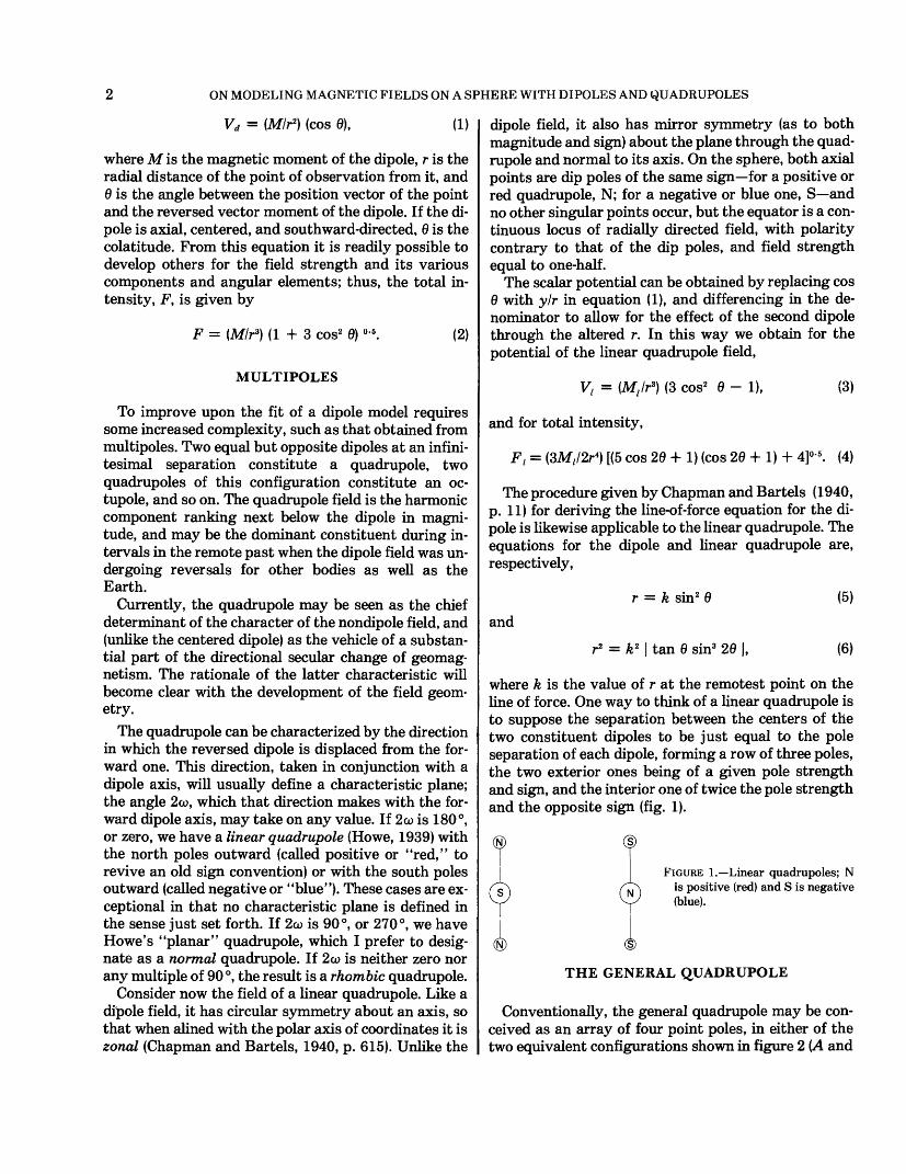
The quadrupole can be characterized by the direction in which the reversed dipole is displaced from the for ward one. This direction, taken in conjunction with a dipole axis, will usually define a characteristic plane; the angle 2co, which that direction makes with the for ward dipole axis, may take on any value. If 2co is 180°, or zero, we have a linear quadrupole (Howe, 1939) with the north poles outward (called positive or "red," to revive an old sign convention) or with the south poles outward (called negative or "blue"). These cases are ex ceptional in that no characteristic plane is defined in the sense just set forth. If 2co is 90°, or 270°, we have Howe's "planar" quadrupole, which I prefer to desig nate as a normal quadrupole. If 2co is neither zero nor any multiple of 90 °, the result is a rhombic quadrupole.
Consider now the field of a linear quadrupole. Like a dipole field, it has circular symmetry about an axis, so that when alined with the polar axis of coordinates it is zonal (Chapman and Bartels, 1940, p. 615). Unlike the
dipole field, it also has mirror symmetry (as to both magnitude and sign) about the plane through the quad rupole and normal to its axis. On the sphere, both axial points are dip poles of the same sign—for a positive or red quadrupole, N; for a negative or blue one, S—and no other singular points occur, but the equator is a con tinuous locus of radially directed field, with polarity contrary to that of the dip poles, and field strength equal to one-half.
The scalar potential can be obtained by replacing cos 0 with ylr in equation (1), and differencing in the de nominator to allow for the effect of the second dipole through the altered r. In this way we obtain for the potential of the linear quadrupole field,
Vt = (MJr3) (3 cos2 0 - 1), (3)
and for total intensity,
F l = (3M,/2r4 ) [(5 cos 20 + 1) (cos 20 + 1) + 4f5 . (4)
The procedure given by Chapman and Bartels (1940, p. 11) for deriving the line-of-force equation for the di pole is likewise applicable to the linear quadrupole. The equations for the dipole and linear quadrupole are, respectively,
andr = k sin2 0
r2 = k 2 | tan 0 sin3 20 |,
(5)
(6)
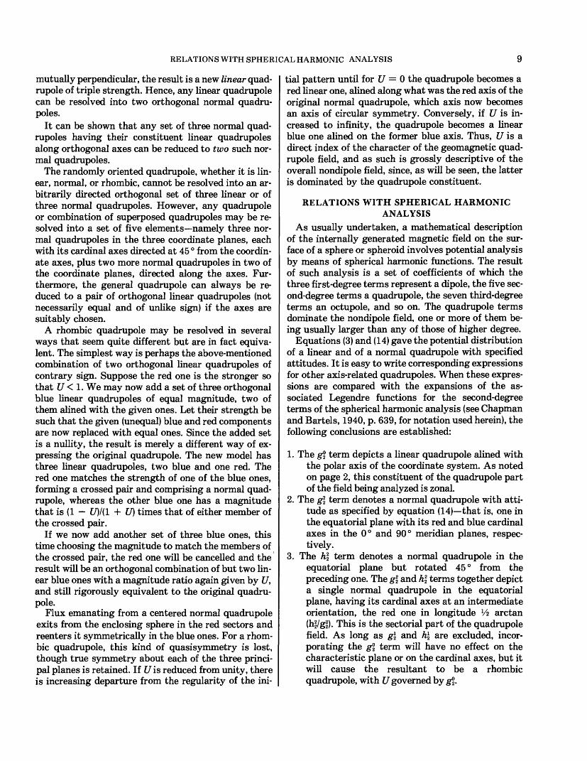
where k is the value of r at the remotest point on the line of force. One way to think of a linear quadrupole is to suppose the separation between the centers of the two constituent dipoles to be just equal to the pole separation of each dipole, forming a row of three poles, the two exterior ones being of a given pole strength and sign, and the interior one of twice the pole strength and the opposite sign (fig. 1).
FIGURE 1.—Linear quadrupoles; N is positive (red) and S is negative (blue).
N) ©
THE GENERAL QUADRUPOLE
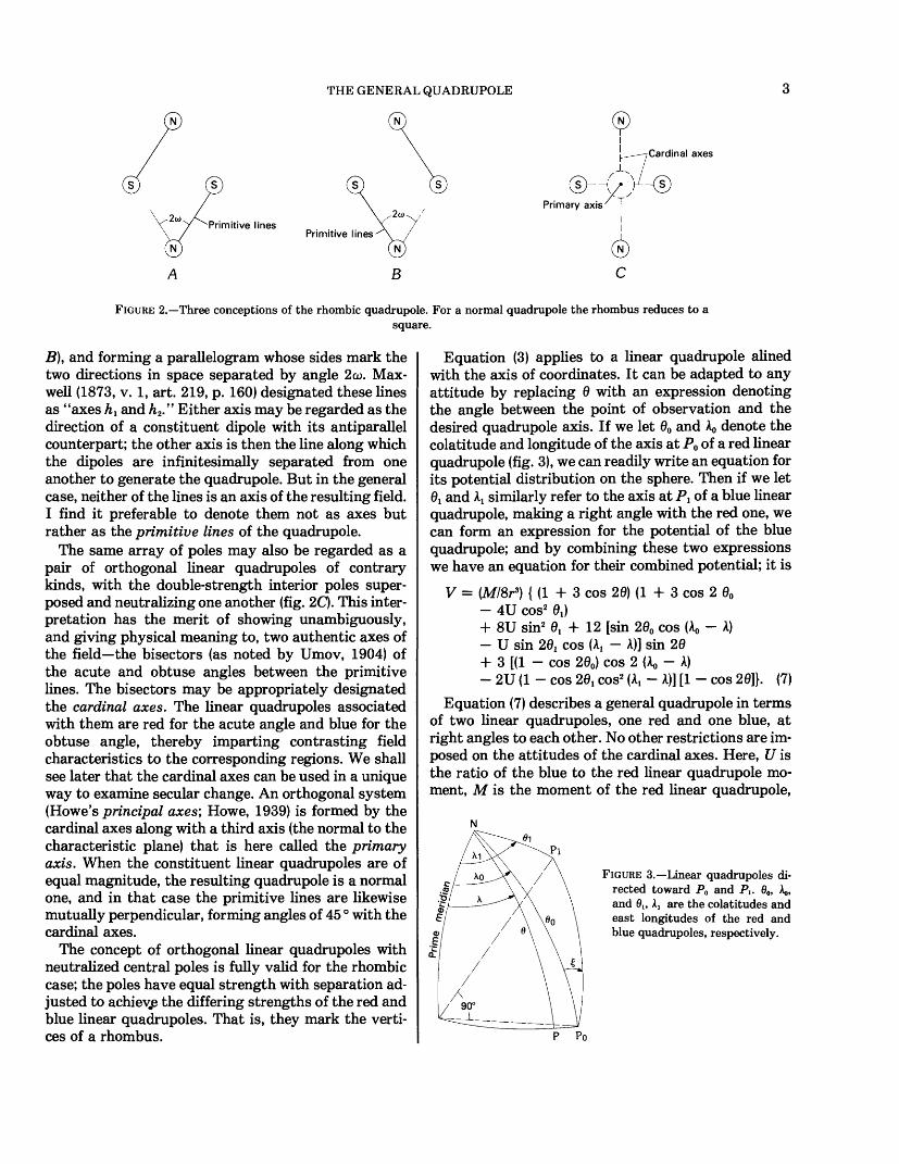
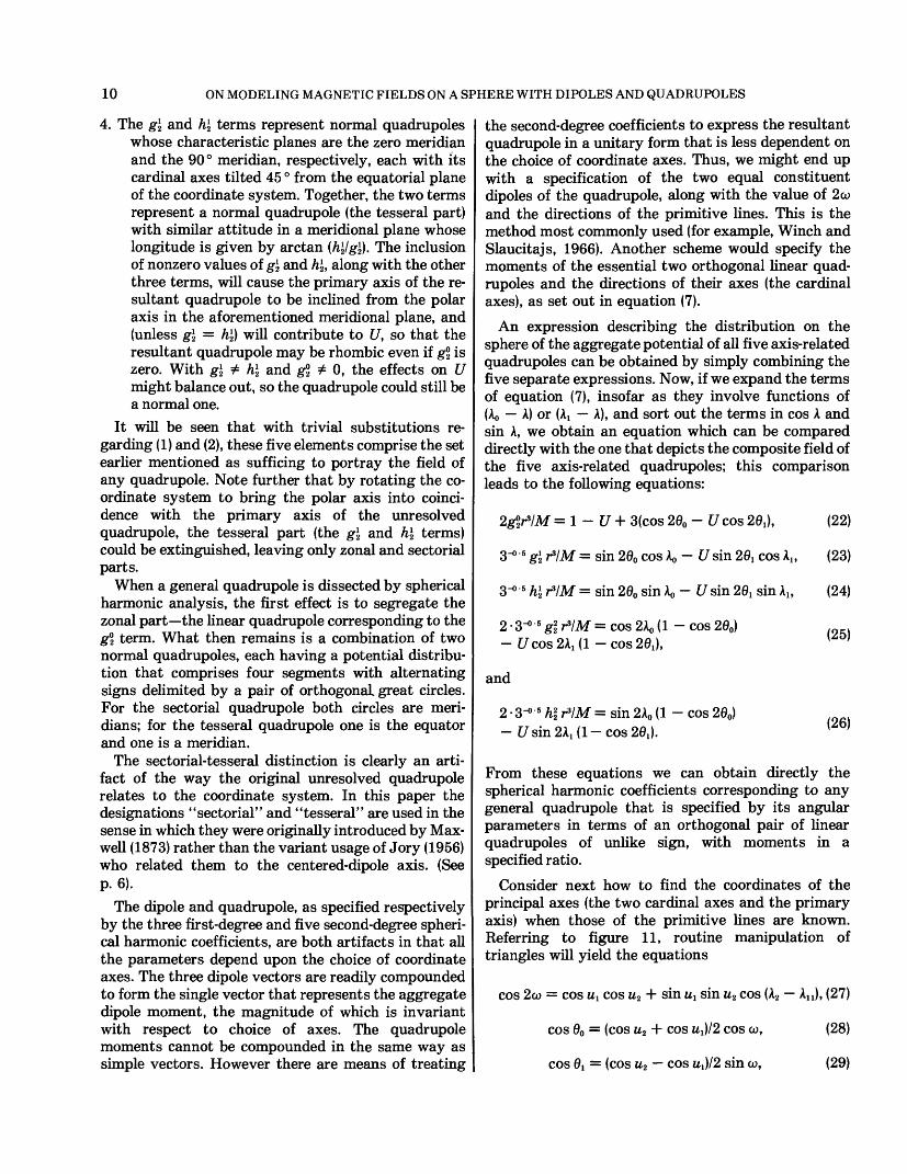
Conventionally, the general quadrupole may be con ceived as an array of four point poles, in either of the two equivalent configurations shown in figure 2 (A and
THE GENERAL QUADRUPOLE^->,N
Primitive linesPrimitive lines
(N)
Primary axis
Cardinal axes
FIGURE 2.—Three conceptions of the rhombic quadrupole. For a normal quadrupole the rhombus reduces to asquare.
B), and forming a parallelogram whose sides mark the two directions in space separated by angle 2co. Max well (1873, v. 1, art. 219, p. 160) designated these lines as "axes hi and h2." Either axis may be regarded as the direction of a constituent dipole with its antiparallel counterpart; the other axis is then the line along which the dipoles are infinitesimally separated from one another to generate the quadrupole. But in the general case, neither of the lines is an axis of the resulting field. I find it preferable to denote them not as axes but rather as the primitive lines of the quadrupole.
The same array of poles may also be regarded as a pair of orthogonal linear quadrupoles of contrary kinds, with the double-strength interior poles super posed and neutralizing one another (fig. 2C). This inter pretation has the merit of showing unambiguously, and giving physical meaning to, two authentic axes of the field—the bisectors (as noted by Umov, 1904) of the acute and obtuse angles between the primitive lines. The bisectors may be appropriately designated the cardinal axes. The linear quadrupoles associated with them are red for the acute angle and blue for the obtuse angle, thereby imparting contrasting field characteristics to the corresponding regions. We shall see later that the cardinal axes can be used in a unique way to examine secular change. An orthogonal system (Howe's principal axes; Howe, 1939) is formed by the cardinal axes along with a third axis (the normal to the characteristic plane) that is here called the primary axis. When the constituent linear quadrupoles are of equal magnitude, the resulting quadrupole is a normal one, and in that case the primitive lines are likewise mutually perpendicular, forming angles of 45 ° with the cardinal axes.
The concept of orthogonal linear quadrupoles with neutralized central poles is fully valid for the rhombic case; the poles have equal strength with separation ad justed to achiev.e the differing strengths of the red and blue linear quadrupoles. That is, they mark the verti ces of a rhombus.
Equation (3) applies to a linear quadrupole alined with the axis of coordinates. It can be adapted to any attitude by replacing 8 with an expression denoting the angle between the point of observation and the desired quadrupole axis. If we let 00 and AQ denote the colatitude and longitude of the axis at P0 of a red linear quadrupole (fig. 3), we can readily write an equation for its potential distribution on the sphere. Then if we let 0t and A! similarly refer to the axis at P^ of a blue linear quadrupole, making a right angle with the red one, we can form an expression for the potential of the blue quadrupole; and by combining these two expressions we have an equation for their combined potential; it is
V = (MISr3 ) { (1 + 3 cos 20) (1 + 3 cos 2 00- 4U cos2 0t )+ 8U sin2 0t + 12 [sin 200 cos (Ao - A)- U sin 20t cos (At - A)] sin 20 + 3 [(1 - cos 200 ) cos 2 (Ao - A)- 2U (1 - cos 20t cos2 (At - A)] [1 - cos 20]}. (7)
Equation (7) describes a general quadrupole in terms of two linear quadrupoles, one red and one blue, at right angles to each other. No other restrictions are im posed on the attitudes of the cardinal axes. Here, U is the ratio of the blue to the red linear quadrupole mo ment, M is the moment of the red linear quadrupole,
PIFIGURE 3.—Linear quadrupoles di
rected toward P0 and Pi. 00, AO, and 0!, A, are the colatitudes and east longitudes of the red and blue quadrupoles, respectively.
P PO
ON MODELING MAGNETIC FIELDS ON A SPHERE WITH DIPOLES AND QUADRUPOLES
and —MU that of the blue one. In this equation the configuration is governed by the five parameters M, U, 00 , 61, and AQ. Parameter Xl is not independent but is re tained to simplify the equation; it is related to the oth ers by
sin (A! — AO) = sin £ /sin 0lt (8)
where £ is the true azimuth of the line extending from P0 to Pl given by
cos f = cos 0!/sin Q0. (9)
If we set 00 and 0: at 90 ° in equation (7), we describe a general quadrupole that is in the equatorial plane; and it may be further particularized by setting AO at zero and A! at 90 °, thus placing the red linear quadrupole in longitude zero and the blue one in longitude 90 °. Equa tion (7) can then be reduced toV = (M/r3) {3[1 - (1 + C7)sin2 A]sin2 0 + U - 1} (10) and this may be further reduced to
V = (d2/4r 3) [3(cos 2A + cos 2co)sin2 0- 2 cos 2co], (11)
where
and
62 = 2 M(l + £7), (12)
cos 2co = (1 - £/)/(! + U). (13)
For a normal quadrupole in the same attitude we need only set U = 1, reducing equation (10) to the form
Vn = (3Mn/r3) (cos 2A sin2 0). (14)
For the quadrupole represented by equation (14), the primitive lines have longitudes of 45° and 135°.
The total intensity of the fields stipulated by equa tions (10) and (14) may be written, respectively, as
F = (3d2 sin 0/2T-4) {sin2 2A + qf cos2 0+ [—cos 2o> esc 0 (15) +(3/2)gnsin0]2}0 - 5,
and
F = (3M/r4) (4 + 5 sin2 0 cos2 2A)°- 5 sin 0, (16)
whereil = cos 2A + cos 2o>.
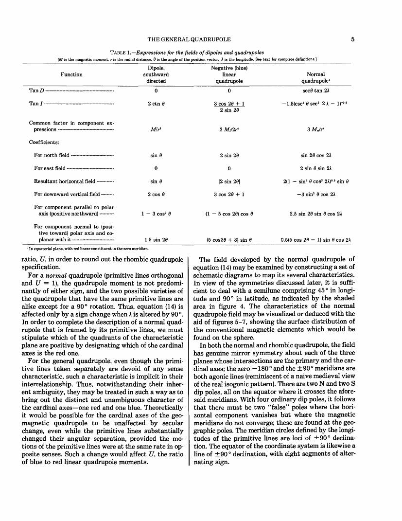
Table 1 compares the expressions for the various ele ments of the field of a dipole, of a linear quadrupole along the polar axis, and of a normal quadrupole in the equatorial plane, as stipulated for equations (1), (3), and (11).
SOME CHARACTERISTICS OF QUADRUPOLE FIELDS
The field of every quadrupole differs fundamentally from a dipole field in that the dipole field is of odd degree and shows asymmetry of sense (inward versus outward) along any straight line going through the center, whereas the quadrupole is of even degree and does not show this asymmetry. A linear quadrupole has a characteristic sign, and a rhombic one may be dominated by the sign of its stronger linear-quad- rupole constituent. The field of a rhombic quadrupole, or of a normal one, has positive and negative aspects, distributed in relation to its cardinal axes.
A general quadrupole cannot be fully described simply by specifying its primitive lines and its (un signed) moment. It is necessary somehow to distin guish between the two sorts of quadrupoles that can exist with identical directions of the primitive lines. The two are related in that the positive aspects of one are exactly matched by the negative of the other. The situation may be examined as follows: If we look at the parallelogram that represents the four point poles of a rhombic quadrupole, the signs of the point poles alter nating as we go round the figure, they may (as has been noted) be coupled in either of two ways to form the two dipoles as shown in figure 2. The angle 2co represents the interior angle of the rhombus at one of the positive or north-seeking poles. Thus, 2cu is unambiguously either obtuse or acute. (The definition given earlier made 2o> the angle from the forward direction of either dipole to the direction in which the other one is dis placed from it.)
If 2o> is obtuse (fig. 2B), the dominant sign of the quadrupole is negative. In this case the points bearing the <S label fall in the obtuse sectors of the characteris tic plane, and the neighboring lines of force are out ward-directed. Each of these statements must be al tered appropriately if 2o> is acute (fig. 2A). To avoid ambiguity, therefore, we need to state whether 2o> is obtuse or acute, indicating which of the angles between the primitive lines is 2o> and which is its supplement.
If instead of the primitive lines one is dealing with their angular bisectors, that is, the cardinal axes (fig. 2C), the distinction between the axes is clear, in that one of them marks the positive (red) and the other the negative (blue) linear quadrupole of an orthogonal pair. The ambiguity now takes a different form. It is now necessary to stipulate not only which is which but also the strength of each, or the strength of one and their
THE GENERAL QUADRUPOLE
TABLE 1.—Expressions for the fields ofdipoles and quadrupoles[M is the magnetic moment, r is the radial distance, 8 is the angle of the position vector, A is the longitude. See text for complete definitions.)
FunctionDipole,
southwarddirected
Negative (blue)linear
quadrupoleNormal
quadrupole1
TanD
Tan/-
Common factor in component ex-
Coefficients:
For north field —
For east field —
Resultant horizontal field
For downward vertical field
For component parallel to polar axis (positive northward)
For component normal to (posi tive toward) polar axis and co- pxQ.iiQ.r witn. it ---------------——«~
0
2ctn 6
M/r3
sin 6
sin 6
2 cos 6
1-3 cos2 6
1.5 sin 26
0
3 cos 202 sin 26
2 sin 26
0
|2 sin 20|
3 cos 26 + 1
(1-5 cos 20) cos 6
(5 cos20 + 3) sin 0
sec0 tan 2A
-1.5(csc2 0 sec2 2A- I)'06
3 M«/r<
sin 20 cos 2A
2 sin 0 sin 2A
2(1 - sin2 0 cos2 2A)° 6 sin 0
-3 sin2 0 cos 2A
2.5 sin 20 sin 0 cos 2A
0.5(5 cos 20 - 1) sin 0 cos 2A1 In equatorial plane, with red linear constituent in the zero meridian.
ratio, U, in order to round out the rhombic quadrupole specification.
For a normal quadrupole (primitive lines orthogonal and U = 1), the quadrupole moment is not predomi nantly of either sign, and the two possible varieties of the quadrupole that have the same primitive lines are alike except for a 90° rotation. Thus, equation (14) is affected only by a sign change when A is altered by 90 °. In order to complete the description of a normal quad rupole that is framed by its primitive lines, we must stipulate which of the quadrants of the characteristic plane are positive by designating which of the cardinal axes is the red one.
For the general quadrupole, even though the primi tive lines taken separately are devoid of any sense characteristic, such a characteristic is implicit in their interrelationship. Thus, notwithstanding their inher ent ambiguity, they may be treated in such a way as to bring out the distinct and unambiguous character of the cardinal axes—one red and one blue. Theoretically it would be possible for the cardinal axes of the geo magnetic quadrupole to be unaffected by secular change, even while the primitive lines substantially changed their angular separation, provided the mo tions of the primitive lines were at the same rate in op posite senses. Such a change would affect £7, the ratio of blue to red linear quadrupole moments.
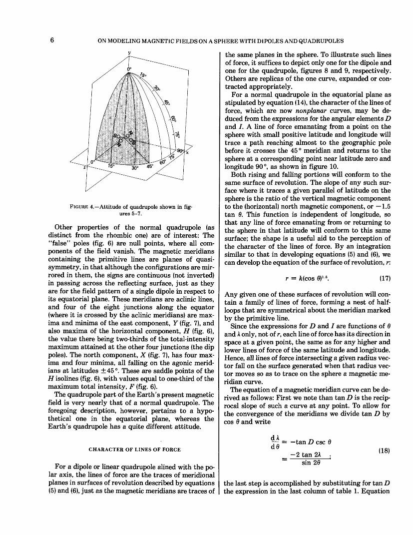
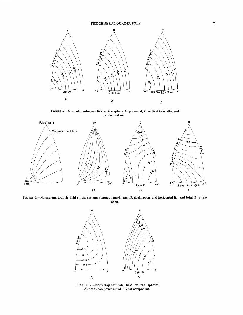
The field developed by the normal quadrupole of equation (14) may be examined by constructing a set of schematic diagrams to map its several characteristics. In view of the symmetries discussed later, it is suffi cient to deal with a semilune comprising 45 ° in longi tude and 90° in latitude, as indicated by the shaded area in figure 4. The characteristics of the normal quadrupole field may be visualized or deduced with the aid of figures 5-7, showing the surface distribution of the conventional magnetic elements which would be found on the sphere.
In both the normal and rhombic quadrupole, the field has genuine mirror symmetry about each of the three planes whose intersections are the primary and the car dinal axes; the zero —180° and the ±90° meridians are both agonic lines (reminiscent of a naive medieval view of the real isogonic pattern). There are two N and two S dip poles, all on the equator where it crosses the afore said meridians. With four ordinary dip poles, it follows that there must be two "false" poles where the hori zontal component vanishes but where the magnetic meridians do not converge; these are found at the geo graphic poles. The meridian circles defined by the longi tudes of the primitive lines are loci of ±90° declina tion. The equator of the coordinate system is likewise a line of ±90° declination, with eight segments of alter nating sign.
ON MODELING MAGNETIC FIELDS ON A SPHERE WITH DIPOLES AND QUADRUPOLES
FIGURE 4.—Attitude of quadrupole shown in fig ures 5-7.
Other properties of the normal quadrupole (as distinct from the rhombic one) are of interest: The "false" poles (fig. 6) are null points, where all com ponents of the field vanish. The magnetic meridians containing the primitive lines are planes of quasi- symmetry, in that although the configurations are mir rored in them, the signs are continuous (not inverted) in passing across the reflecting surface, just as they are for the field pattern of a single dipole in respect to its equatorial plane. These meridians are aclinic lines, and four of the eight junctions along the equator (where it is crossed by the aclinic meridians) are max ima and minima of the east component, Y (fig. 7), and also maxima of the horizontal component, H (fig. 6), the value there being two-thirds of the total-intensity maximum attained at the other four junctions (the dip poles). The north component, X (fig. 7), has four max ima and four minima, all falling on the agonic merid ians at latitudes ±45°. These are saddle points of the H isolines (fig. 6), with values equal to one-third of the maximum total intensity, F (fig. 6).
The quadrupole part of the Earth's present magnetic field is very nearly that of a normal quadrupole. The foregoing description, however, pertains to a hypo thetical one in the equatorial plane, whereas the Earth's quadrupole has a quite different attitude.
CHARACTER OF LINES OF FORCE
For a dipole or linear quadrupole alined with the po lar axis, the lines of force are the traces of meridional planes in surfaces of revolution described by equations (5) and (6), just as the magnetic meridians are traces of
the same planes in the sphere. To illustrate such lines of force, it suffices to depict only one for the dipole and one for the quadrupole, figures 8 and 9, respectively. Others are replicas of the one curve, expanded or con tracted appropriately.
For a normal quadrupole in the equatorial plane as stipulated by equation (14), the character of the lines of force, which are now nonplanar curves, may be de duced from the expressions for the angular elements D and /. A line of force emanating from a point on the sphere with small positive latitude and longitude will trace a path reaching almost to the geographic pole before it crosses the 45 ° meridian and returns to the sphere at a corresponding point near latitude zero and longitude 90 °, as shown in figure 10.
Both rising and falling portions will conform to the same surface of revolution. The slope of any such sur face where it traces a given parallel of latitude on the sphere is the ratio of the vertical magnetic component to the (horizontal) north magnetic component, or —1.5 tan 9. This function is independent of longitude, so that any line of force emanating from or returning to the sphere in that latitude will conform to this same surface; the shape is a useful aid to the perception of the character of the lines of force. By an integration similar to that in developing equations (5) and (6), we can develop the equation of the surface of revolution, r:
r = k(cos 0)15. (17)
Any given one of these surfaces of revolution will con tain a family of lines of force, forming a nest of half- loops that are symmetrical about the meridian marked by the primitive line.
Since the expressions for D and / are functions of 9 and A only, not of r, each line of force has its direction in space at a given point, the same as for any higher and lower lines of force of the same latitude and longitude. Hence, all lines of force intersecting a given radius vec tor fall on the surface generated when that radius vec tor moves so as to trace on the sphere a magnetic me ridian curve.
The equation of a magnetic meridian curve can be de rived as follows: First we note than tan D is the recip rocal slope of such a curve at any point. To allow for the convergence of the meridians we divide tan D by cos 9 and write
dAd0 —tan D esc 9
—2 tan 2A . sin 29
(18)
the last step is accomplished by substituting for tan D the expression in the last column of table 1. Equation
THE GENERAL QUADBUPOLE
FIGURE 5.—Normal-quadrupole field on the sphere: V, potential; Z, vertical intensity; andI, inclination.
'False" pole
Magnetic meridians
D(5 cos2 2X + 4)0.5
F2.0
FIGURE 6.—Normal-quadrupole field on the sphere: magnetic meridians; D, declination; and horizontal (H) and total (F) inten sities.
X
FIGURE 7.—Normal-quadrupole field on the sphere: X, north component; and Y, east component.

ON MODELING MAGNETIC FIELDS ON A SPHERE WITH DIPOLES AND QUADRUPOLES
Axis of symmetry
Plane of quasisymmetry
FIGURE 8.—Dipole field line.
FIGURE 9.—Linear-quadrupole field line.
(18) states the basic condition that a magnetic meri dian curve must satisfy. It is readily integrated to give
sin 2A tan2 0 = k, (19)
where the constant k is the value of tan2 9 for A = 45°—that is, for the minimum 0. Thus (19) is the equa tion of the magnetic meridian curves on the sphere; it also describes in space the singly curved surfaces whose intersections with the surfaces of revolution de scribed by equation (17) are the lines of force of a nor mal quadrupole having its attitude defined by equa tion (14).
INTERCONVERSION OF QUADRUPOLES
With U = 0, equation (7) gives the potential of a red linear quadrupole:
V = (M/8r3) {(1 + 3 cos 20)(1 + 3 cos 200 ) + 12[sin 200 sin 20 cos(Ao - A)] + 3[(1 - cos 200)cos 2(Ao - A)] (1 - cos 20)}. (20)
Iat0° ,long 90°
< Equatorial plane-Iat0° long 0°
FIGURE 10.—Normal-quadrupole field line.
Now if we set 00 and A,, first at 90 ° and zero, respec tively, then both at 90 °, then both at zero, we have ex pressions for the potentials of three orthogonal linear quadrupoles, and their sum is found to be
V, = (M/8r3) {(4 - 2 - 2)(1 + 3 cos 20) + 3(2 cos 2A)(1 - cos 20) + 3[2(-cos 2A)) (1- cos 20)}=0 (21)
That is, the combination of three equal, orthogonal lin ear quadrupoles of the same sign is a nullity. Con sequently, two equal mutually perpendicular linear quadrupoles are rigorously equivalent to a third one of the contrary sign (and of the same magnitude), or thogonal with both given ones. It follows that if two normal quadrupoles of equal strength are combined in such a way that their constituent linear quadrupoles of one sign coincide and those of the other sign are
RELATIONS WITH SPHERICAL HARMONIC ANALYSIS
mutually perpendicular, the result is a new linear quad- rupole of triple strength. Hence, any linear quadrupole can be resolved into two orthogonal normal quadru- poles.
It can be shown that any set of three normal quad- rupoles having their constituent linear quadrupoles along orthogonal axes can be reduced to two such nor mal quadrupoles.
The randomly oriented quadrupole, whether it is lin ear, normal, or rhombic, cannot be resolved into an ar bitrarily directed orthogonal set of three linear or of three normal quadrupoles. However, any quadrupole or combination of superposed quadrupoles may be re solved into a set of five elements—namely three nor mal quadrupoles in the three coordinate planes, each with its cardinal axes directed at 45 ° from the coordin ate axes, plus two more normal quadrupoles in two of the coordinate planes, directed along the axes. Fur thermore, the general quadrupole can always be re duced to a pair of orthogonal linear quadrupoles (not necessarily equal and of unlike sign) if the axes are suitably chosen.
A rhombic quadrupole may be resolved in several ways that seem quite different but are in fact equiva lent. The simplest way is perhaps the above-mentioned combination of two orthogonal linear quadrupoles of contrary sign. Suppose the red one is the stronger so that U < 1. We may now add a set of three orthogonal blue linear quadrupoles of equal magnitude, two of them alined with the given ones. Let their strength be such that the given (unequal) blue and red components are now replaced with equal ones. Since the added set is a nullity, the result is merely a different way of ex pressing the original quadrupole. The new model has three linear quadrupoles, two blue and one red. The red one matches the strength of one of the blue ones, forming a crossed pair and comprising a normal quad rupole, whereas the other blue one has a magnitude that is (1 — £/)/(! + U) times that of either member of the crossed pair.
If we now add another set of three blue ones, this time choosing the magnitude to match the members of the crossed pair, the red one will be cancelled and the result will be an orthogonal combination of but two lin ear blue ones with a magnitude ratio again given by £7, and still rigorously equivalent to the original quadru pole.
Flux emanating from a centered normal quadrupole exits from the enclosing sphere in the red sectors and reenters it symmetrically in the blue ones. For a rhom bic quadrupole, this kind of quasisymmetry is lost, though true symmetry about each of the three princi pal planes is retained. If U is reduced from unity, there is increasing departure from the regularity of the ini
tial pattern until for U = 0 the quadrupole becomes a red linear one, alined along what was the red axis of the original normal quadrupole, which axis now becomes an axis of circular symmetry. Conversely, if U is in creased to infinity, the quadrupole becomes a linear blue one alined on the former blue axis. Thus, U is a direct index of the character of the geomagnetic quad rupole field, and as such is grossly descriptive of the overall nondipole field, since, as will be seen, the latter is dominated by the quadrupole constituent.
RELATIONS WITH SPHERICAL HARMONICANALYSIS
As usually undertaken, a mathematical description of the internally generated magnetic field on the sur face of a sphere or spheroid involves potential analysis by means of spherical harmonic functions. The result of such analysis is a set of coefficients of which the three first-degree terms represent a dipole, the five sec ond-degree terms a quadrupole, the seven third-degree terms an octupole, and so on. The quadrupole terms dominate the nondipole field, one or more of them be ing usually larger than any of those of higher degree.
Equations (3) and (14) gave the potential distribution of a linear and of a normal quadrupole with specified attitudes. It is easy to write corresponding expressions for other axis-related quadrupoles. When these expres sions are compared with the expansions of the as sociated Legendre functions for the second-degree terms of the spherical harmonic analysis (see Chapman and Bartels, 1940, p. 639, for notation used herein), the following conclusions are established:
1. The gl term depicts a linear quadrupole alined with the polar axis of the coordinate system. As noted on page 2, this constituent of the quadrupole part of the field being analyzed is zonal.
2. The gl term denotes a normal quadrupole with atti tude as specified by equation (14)—that is, one in the equatorial plane with its red and blue cardinal axes in the 0° and 90° meridian planes, respec tively.
3. The h\ term denotes a normal quadrupole in the equatorial plane but rotated 45° from the preceding one. The g\ and h\ terms together depict a single normal quadrupole in the equatorial plane, having its cardinal axes at an intermediate orientation, the red one in longitude Vi arctan (h|/g|). This is the sectorial part of the quadrupole field. As long as g\ and h\ are excluded, incor porating the g\ term will have no effect on the characteristic plane or on the cardinal axes, but it will cause the resultant to be a rhombic quadrupole, with U governed by gl.
10 ON MODELING MAGNETIC FIELDS ON A SPHERE WITH DIPOLES AND QUADRUPOLES
4. The g\ and h\ terms represent normal quadrupoles whose characteristic planes are the zero meridian and the 90° meridian, respectively, each with its cardinal axes tilted 45 ° from the equatorial plane of the coordinate system. Together, the two terms represent a normal quadrupole (the tesseral part) with similar attitude in a meridional plane whose longitude is given by arctan (h2lg\). The inclusion of nonzero values of g\ and h\, along with the other three terms, will cause the primary axis of the re sultant quadrupole to be inclined from the polar axis in the aforementioned meridional plane, and (unless g\ = h\] will contribute to U, so that the resultant quadrupole may be rhombic even if g\ is zero. With g\ ? h\ and #2^0, the effects on U might balance out, so the quadrupole could still be a normal one.
It will be seen that with trivial substitutions re garding (1) and (2), these five elements comprise the set earlier mentioned as sufficing to portray the field of any quadrupole. Note further that by rotating the co ordinate system to bring the polar axis into coinci dence with the primary axis of the unresolved quadrupole, the tesseral part (the g\ and h\ terms) could be extinguished, leaving only zonal and sectorial parts.
When a general quadrupole is dissected by spherical harmonic analysis, the first effect is to segregate the zonal part—the linear quadrupole corresponding to the g\ term. What then remains is a combination of two normal quadrupoles, each having a potential distribu tion that comprises four segments with alternating signs delimited by a pair of orthogonal great circles. For the sectorial quadrupole both circles are meri dians; for the tesseral quadrupole one is the equator and one is a meridian.
The sectorial-tesseral distinction is clearly an arti fact of the way the original unresolved quadrupole relates to the coordinate system. In this paper the designations "sectorial" and "tesseral" are used in the sense in which they were originally introduced by Max well (1873) rather than the variant usage of Jory (1956) who related them to the centered-dipole axis. (See p. 6).
The dipole and quadrupole, as specified respectively by the three first-degree and five second-degree spheri cal harmonic coefficients, are both artifacts in that all the parameters depend upon the choice of coordinate axes. The three dipole vectors are readily compounded to form the single vector that represents the aggregate dipole moment, the magnitude of which is invariant with respect to choice of axes. The quadrupole moments cannot be compounded in the same way as simple vectors. However there are means of treating
the second-degree coefficients to express the resultant quadrupole in a unitary form that is less dependent on the choice of coordinate axes. Thus, we might end up with a specification of the two equal constituent dipoles of the quadrupole, along with the value of 2cu and the directions of the primitive lines. This is the method most commonly used (for example, Winch and Slaucitajs, 1966). Another scheme would specify the moments of the essential two orthogonal linear quad rupoles and the directions of their axes (the cardinal axes), as set out in equation (7).
An expression describing the distribution on the sphere of the aggregate potential of all five axis-related quadrupoles can be obtained by simply combining the five separate expressions. Now, if we expand the terms of equation (7), insofar as they involve functions of (Ao — A) or (A! — A), and sort out the terms in cos A and sin A, we obtain an equation which can be compared directly with the one that depicts the composite field of the five axis-related quadrupoles; this comparison leads to the following equations:
(22)
(23)
(24)
(25)
= 1 - U + 3(cos 200 - t/cos 20,),
3-° ' 5 g\ rVM = sin 200 cos AO - U sin 20, cos Alt
3-° 5 h\ rVM = sin 200 sin AO - U sin 20, sin A,,
2 .3-0 5 gi ,3/M _ cos 2Ao (i _ Cos 200 ) - t/cos2A, (1 -cos 20,),
and
2 • 3-°' 6 Af rVM = sin 2A,, (1 - cos 200) - t/sin2A,(l-cos20i). (26)
From these equations we can obtain directly the spherical harmonic coefficients corresponding to any general quadrupole that is specified by its angular parameters in terms of an orthogonal pair of linear quadrupoles of unlike sign, with moments in a specified ratio.
Consider next how to find the coordinates of the principal axes (the two cardinal axes and the primary axis) when those of the primitive lines are known. Referring to figure 11, routine manipulation of triangles will yield the equations
cos 2o> = cos HI cos u2 + sin u, sin u2 cos (A2 — A,,), (27)
cos 00 = (cos u2 + cos u,)/2 cos cu, (28)
cos 0, = (cos u2 — cos u,)/2 sin co, (29)
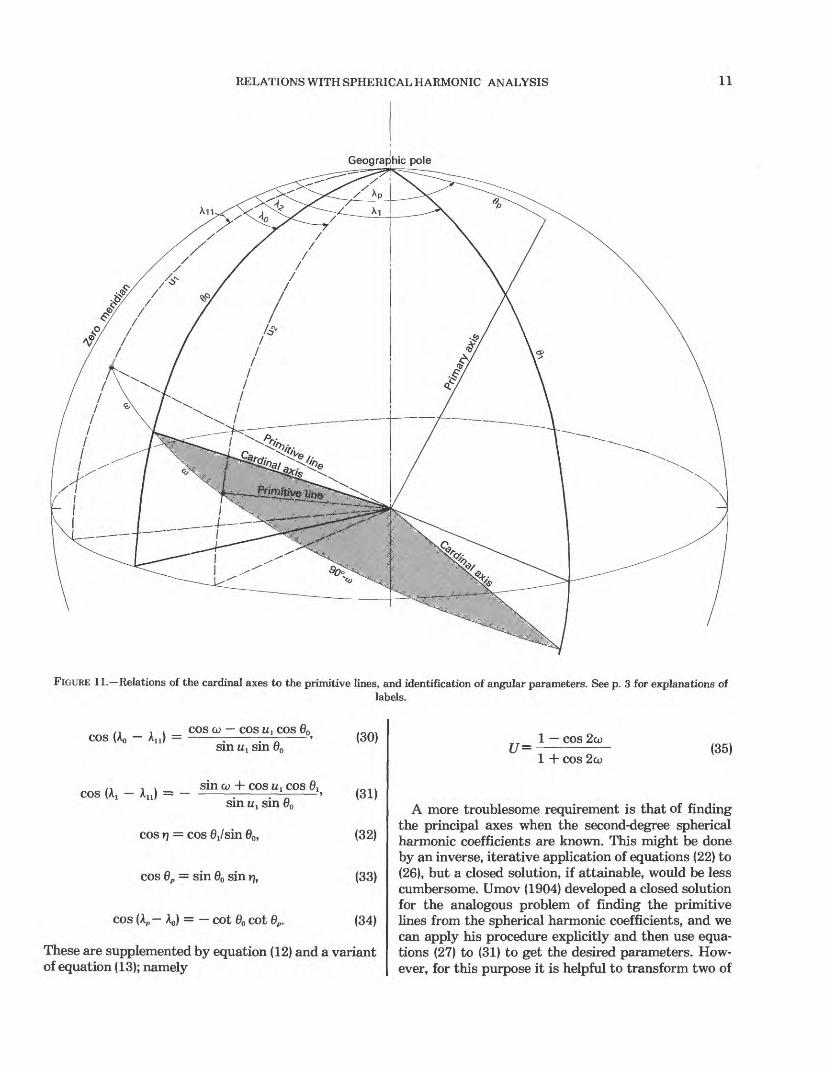
RELATIONS WITH SPHERICAL HARMONIC ANALYSIS 11
FIGURE 11.—Relations of the cardinal axes to the primitive lines, and identification of angular parameters. See p. 3 for explanations oflabels.
COS (An — A,,) =_ COS CO — COS I/! COS 00——————;——————;——-—————'
sin M! sin 60 (30)
COS (A, — _ sin co + cos ul cos 0t — ————:———:—o———' sin 1/1 sin 60
cos Y] = cos
cos 6P = sin 60 sin rj,
cos (Ap — AO) = — cot 00 cot 6P.
(32)
(33)
(34)
These are supplemented by equation (12) and a variant of equation (13); namely
U= 1 — cos 2co 1 + cos 2co
(35)
A more troublesome requirement is that of finding the principal axes when the second-degree spherical harmonic coefficients are known. This might be done by an inverse, iterative application of equations (22) to (26), but a closed solution, if attainable, would be less cumbersome. Umov (1904) developed a closed solution for the analogous problem of finding the primitive lines from the spherical harmonic coefficients, and we can apply his procedure explicitly and then use equa tions (27) to (31) to get the desired parameters. How ever, for this purpose it is helpful to transform two of
12 ON MODELING MAGNETIC FIELDS ON A SPHERE WITH DIPOLES AND QUADRUPOLES
his equations (the last two in the group he labeled "I") into the form
cot MI = x =h21 cos AI —
and
cot uz = y =
., .- ,, 1.5M2 sm(A2 —
g21 sinA2 — h21 cos A2 1.5M2 sin(A2 — Aj)
(36)
(37)
Umov's procedure involves the numerical solution of a cubic equation having three real roots, the well-known irreducible case. Although algebraic solution of this cubic is impossible, a trigonometric procedure may be used (Dickson, 1922, §47). Only one of the resulting roots will yield a meaningful value of cos 2co.
QUADRUPOLE SECULAR CHANGE AND ITS CONSERVATIVE ASPECT
A distinction that is rather technical, yet still funda mental, may be recognized between the dipole on the one hand and the quadrupole and higher multipoles on the other. Under secular change, the dipole axis could move on the sphere along a track which might or might not trace a great-circle path. Since there is but one axis, its instantaneous direction of motion contains no clue to the curvature of the path it traces out. Only by comparing the motion at two successive epochs could we observe such curvature and locate the center of gy ration. A multipole, on the other hand, has at least three axes (unless it is a linear one). By assessing the motion of any two of its axes we can fix the center of gyration describing the drift from the secular-change data of a single epoch.
It is well known that the secular change shows pre dominantly regional characteristics, although it is now also accepted that an important part must have a glob al character. To evaluate and isolate the global fea tures may be a vital step in gaining a fuller under standing of the remaining constituents.
What about the dipole field? The centered dipole with its wandering and reversals is important in paleo- magnetic studies. However, recognition is increasing that dwelling exclusively on the dipole presents the hazard of a simplistic approach that can ignore signifi cant phenomena (Harrison, 1975). Here, our concern with the secular change pertains to structure observed in historic times; and in this context the secular drift of the dipole is difficult to pin down. The centered dipole, though varying somewhat in strength, is almost fixed
in direction. That is, its very slow drift in position con tributes a nearly negligible part of the overall patterns of the secular-change field. Thus, the multipoles (terms of degree 2 or higher) must be the bearers of the domi nant features of the secular-change configurations.
The study of the character of secular change thus seems to link up with the study of the nondipole field—a task that has more than one approach. A cur rently favored and promising technique is to model the nondipole field (or even the entire field) by postulating an array of current loops just within the core bound ary—or as more expediently approximated, by assum ing a distribution of satellite dipoles. However, if we seek to focus on the global aspect of secular change, it may be also instructive to examine the nondipole field by the alternative approach of studying the behavior of the centered multipoles of higher complexity. In this approach, the quadrupole, as the dominant constituent of the nondipole field, is most likely to epitomize any global features that may be present in the secular change. Hence, the quadrupole is clearly the first thing to study. The techniques developed may be adaptable to some of the higher multipoles as well. The secular- change problem, then, offers a distinct and cogent in centive for probing the character and behavior of the geomagnetic quadrupole.
The quadrupole may exhibit the effects of secular change in one or more of the following ways: (1) the combined quadrupole moment may change; (2) the three principal axes may undergo systematic rotation about a fourth axis; or (3) Umay change. If the effect is (2), the primitive lines would necessarily reflect it; but these lines would be affected in a different way by any change in U— they would undergo opposing drifts in the characteristic plane, which might obscure the sit uation. To study the global constituent we should dis tinguish between effects (2) and (3).
With the lapse of time, rotation of a field having ax ial symmetry, such as that of a centered dipole or of a linear quadrupole, will be scarcely perceptible in the pattern of the change parameters unless the axis of such rotation makes a considerable angle with the axis of symmetry; but rotation of the field of a normal quadrupole, or of a rhombic one that is not much dif ferent from a normal one, will be apparent no matter where the axis of rotation lies. That is, the surface field on the sphere has a two-dimensional configuration, so that any kind of rotation is bound to displace some of the zero lines of the pattern. Consequently, if the secular change has any global constituent we may ex pect it to be prominently manifested as an angular drift of the principal axes of the quadrupole, and perhaps of the higher multipoles as well.

RELATIONS WITH SPHERICAL HARMONIC ANALYSIS 13
THE ECCENTRIC DIPOLE
The resultant of the vectors represented by the three first-degree terms of the spherical-harmonic expansion is the well-known inclined, centered dipole of best fit. It was shown by Schmidt (1918) that an eccentric dipole is uniquely defined by these same three terms in conjunction with the five second-degree terms (those of the quadrupole), and that this eccentric dipole has the same moment and the same attitude in space as the centered dipole based on the first-degree terms alone.
Six parameters suffice to describe Schmidt's eccen tric dipole. These could be, for example, the three or thogonal components of the centered dipole and the three orthogonal components of the vector stipulating the displacement of the eccentric dipole away from the Earth's center. The field of the eccentric dipole is not identical with that of the combined quadrupole and centered dipole with which it corresponds (governed by eight coefficients). Nevertheless, it is of some interest to consider just how the displacement of the eccentric dipole from the center is affected by manipulating the quadrupole.
When a linear quadrupole is superimposed on a di pole (both centered in the sphere), the eccentric dipole that best approximates the composite field is one that is displaced, (1) along the dipole axis if the quadrupole is either alined with or perpendicular to that axis, or (2) perpendicular to the dipole axis if the quadrupole is tilted 45 ° from it. The effect of a normal quadrupole (or of a rhombic one) may be examined by considering the separate effects of its constituent linear quadrupoles.
FERTILE AND STERILE PARTS OF THE QUADRUPOLE
We have seen how the general quadrupole is resolved (by spherical harmonic analysis) into five constituents governed by the coordinate axes. A similar resolution could be conducted relative to any set of orthogonal axes. Thus, if we define the polar axis to coincide with the centered dipole, and define the other axes so that one of the resulting planes would contain the displace ment vector of the eccentric dipole, the resolution would break up the quadrupole into "fertile" and "sterile" parts, in the sense that the fertile parts would be responsible for the displacement of the dipole and the sterile parts would not, though of course they would still be a necessary part of the description of the original quadrupole field. The sterile parts ((2) and (3), p. 9) make up a normal quadrupole in the equatorial plane of the dipole, whereas the fertile parts ((1), (4), p. 9) constitute a rhombic quadrupole in the plane de fined by the dipole axis and the displacement vector. Separately, the fertile constituents comprise a linear
part whose axis coincides with the dipole axis and a normal part in the plane just mentioned, with its car dinal axes 45 ° from the dipole axis. The displacement of the dipole along its axis is proportional to the strength of the linear part, but the displacement of the dipole normal to its axis is proportional to the strength of the normal part.
If the field subjected to spherical harmonic analysis happens to be that of an eccentric dipole, the sterile part of the quadrupole will be zero. Further, if the dipole is displaced only along its axis (if it is a radial dipole), the quadrupole will be only a linear one along the same axis. If the dipole is displaced only in its equatorial plane, the quadrupole will be a normal one coplanar with the dipole, with its cardinal axes at 45 ° with the dipole axis. (This is approximately true of the Earth's field.)
It is now clear why Chargoy (1950) found that if one deducts from the geomagnetic field its eccentric-dipole component, the residuum has for its quadrupole part a normal quadrupole in the plane perpendicular to the dipole. As noted by Macht (1950), this result is not a fortuitous circumstance of the geomagnetic field but is a mathematical necessity; for the dipole by its eccen tricity allows for a certain quadrupole constituent, and the only remaining quadrupole constituent is a normal one in the equatorial plane defined by the dipole.
When the sterile part of the quadrupole is zero, the six parameters of the eccentric dipole describe a field corrresponding as nearly as possible to that of the eight parameters of the centered-dipole-plus-quadru- pole model, in the sense that no quadrupole component is neglected. The eccentric-dipole field, of course, em bodies not only the centered dipole plus the fertile quadrupole, but also an infinite series of higher multipole terms, and there is no reason to expect these components to be at all similar, or even related, to the terms of corresponding degree in the original spherical harmonic analysis, since the eccentric-dipole dis placement is governed strictly by the parameters of the fertile quadrupole alone. Only if that displacement is large, however, would a large number of multipole terms be required to approximate well the eccentric- dipole field.
The eccentric dipole specified by Schmidt's (1918) procedure, based on the first eight terms of the spheri cal harmonic expansion, is the dipole that best sim ulates the field represented by those terms. It is usual to consider that this dipole is likewise the one of best fit for the field of higher approximation represented by the more detailed analysis. Bartels (1936, p. 230) wrote, "If the field of a magnet like the Earth is to be approximated by that of a dipole not necessarily
14 ON MODELING MAGNETIC FIELDS ON A SPHERE WITH DIPOLES AND QUADRUPOLES
situated at the Earth's center, it can be shown that there is one point C in the magnet, called the magnetic center, which gives the most suitable location." Schmidt's eccentric dipole is defined so as to fall at the magnetic center, defined originally by Kelvin (1872, p. 374).
As a matter of fact, C is usually specified to be de termined solely by the first- and second-degree terms; thus it is not necessarily the site of the best fitting dipole if the higher terms are to be considered. This may be seen most readily if we simplify the circum stances by supposing that the field being modeled is zonal, that is, symmetrical about the axis of coor dinates, hence capable of being completely depicted by the terms of various degrees of order 0. In this case all terms are zero except #?, gl, gl, — gm and Schmidt's ec centric dipole will be displaced along the axis through a distance determined by gl. But if higher terms are considered, it is clear that each term of even degree will represent an incremental distribution of potential having two N or two S dip poles at the ends of the axis (like the N or S dip poles of the quadrupole term) and will result in a separate and independent displacement of the dipole along its axis; so the dipole that best ap proximates the composite field of the whole series will be displaced from the center by a greater or smaller distance than the one that depends only on the terms of degrees 1 and 2, unless it happens that the displacements due to the higher terms add up to zero.
The fallacy of regarding the eccentric dipole deter mined from the first- and second-degree terms as the dipole that best fits the actual field has also been pointed out by Bochev (1965). However, the discrep ancy may well be so small as to have theoretical in terest only.
OTHER REMARKS CONCERNING ECCENTRIC DIPOLES
Given the six parameters of any eccentric dipole, one can evaluate, by means of an equation given by Hur- witz (1960), those of its nearest equivalent centered- dipole-plus-quadrupole combination, thus finding the spherical harmonic coefficients of degrees 1 and 2 (of the eccentric-dipole field) without the necessity of con ducting a spherical harmonic analysis. (The Hurwitz equation is not restricted to the first two degrees but these are of special interest here.) And if more than one eccentric dipole were assumed, the resulting coeffi cients could be determined for each one, and they could be summed to get those of the synthetic field gen erated by all the dipoles, insofar as it was reproducible in terms of eight coefficients. However, the individual quadrupoles so derived would evidently be of a special character in that each of them would be a rhombic one
in the plane defined by the particular dipole and its displacement vector.
This constraint on the second-degree terms (limiting the quadrupole to a plane established by the eccentric dipole) would be operative no matter how the coeffi cients were derived and no matter how many higher degree coefficients were also determined. It implies in terrelations among the five second-degree coefficients, such that g\ and h\ would vanish if the coordinate axis were chosen to conform with the dipole. Nevertheless, such a capability is a useful tool for studying satellite- dipole field models.
The quadrupole so constrained is coplanar with the dipole. The longitude of its characteristic plane (again assuming the coordinate system chosen to conform with the dipole) is equal to arctan (h\lg$; and if in ad dition gl is zero, the quadrupole is a normal one. Alter natively, if all the second-degree terms except gl are zero, the dipole and quadrupole (now linear) are on the coordinate axis. More generally, for any radial dipole the quadrupole will be a linear one coaxial with it.
Although the five second-degree coefficients so de rived constitute a unique and correct reflection of any given eccentric dipole, they do not fully depict the quadrupole aspect of any more generalized field of which the eccentric dipole may be only an approxima tion, inasmuch as they fail to incorporate the former's sterile quadrupole constituent. Assuming a given set of real data subjected to spherical harmonic analysis, its quadrupole will contain not only the fertile constit uent disclosed by the eccentric-dipole approach but also the sterile part, which is lost through that ap proach. For a field free of artificial constraints, know ledge of the six parameters of the eccentric dipole could not suffice to recover the eight parameters of the slightly more detailed dipole-plus-quadrupole descrip tion.
APPLICATION TO EXTANT MODELS
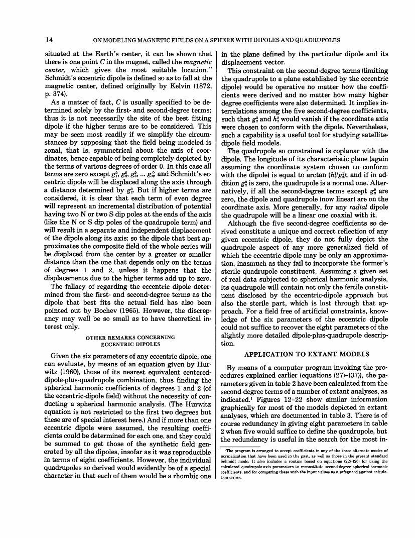
By means of a computer program invoking the pro cedures explained earlier (equations (27)-(37)), the pa rameters given in table 2 have been calculated from the second-degree terms of a number of extant analyses, as indicated. 1 Figures 12-22 show similar information graphically for most of the models depicted in extant analyses, which are documented in table 3. There is of course redundancy in giving eight parameters in table 2 when five would suffice to define the quadrupole, but the redundancy is useful in the search for the most in-
J The program is arranged to accept coefficients in any of the three alternate modes of normalization that have been used in the past, as well as those in the present standard Schmidt mode. It also includes a routine based on equations (22)-(26) for using the calculated quadrupole-axis parameters to reconstitute second-degree spherical-harmonic coefficients, and for comparing these with the input values as a safeguard against calcula tion errors.
APPLICATION TO EXTANT MODELS 15
TABLE 2—Quadrupole parameters of specific field models[60 , Ol , AO and Aj are the coordinates of the cardinal axes; 6P , Ap are the coordinates of the primitive axis; U is the ratio of the quadrupole moments;
d2 = 2M (1 + U); parameters in degrees and minutes]
Model — - —
Epoch ———
Barraclough Gauss
1650 1835
Dyson- Furner- AWC-70 AWC-70 Fanselau
1922 1937.5 1970
IGRF
1965
Parameter:
Ul/2(J2
52 0089 3660 30
205 5052 00
322 00
6.4032417.9
46 3124 3256 24
153 3662 01
264 16
0.8481938.9
57 594 22
45 30132 1761 30
254 32
0.9662143.5
59 11355 4139 57
131 0567 13
251 10
0.9502290.5
61 58347 2634 24
128 2871 44
247 19
1.132516.2
61 14348 1535 21128 5771 15
247 31
1.1342461.2
structive way to depict the secular change of the geo magnetic quadrupole. The primary axis is of interest because it is the normal to the quadrupole's charac teristic plane and hence defines that plane with only two parameters. Both cardinal axes lie in that plane and mark those points on the surface of the sphere where the quadrupole field is normal to the surface. As
we have seen, these points are the authentic surface dip poles of the quadrupole field (N and S).
Note that for the recent models, the colatitude and longitude of the red axis (00 and AJ place it off the At lantic coast of Morocco; those of the blue axis (61 and AJ place it in Amur, Siberia; and those of the primary axis (6P and Ap ) place it in the Pacific Ocean about 120
120° 105° 90° 75'
FIGURE 12.—Drift of the primary axis of the geomagnetic quadrupole since 1550. Letters refer to the groups listed in table 3.
16114'
ON MODELING MAGNETIC FIELDS ON A SPHERE WITH DIPOLES AND QUADRUPOLES
112° 110° 108° 106°W.
18° N
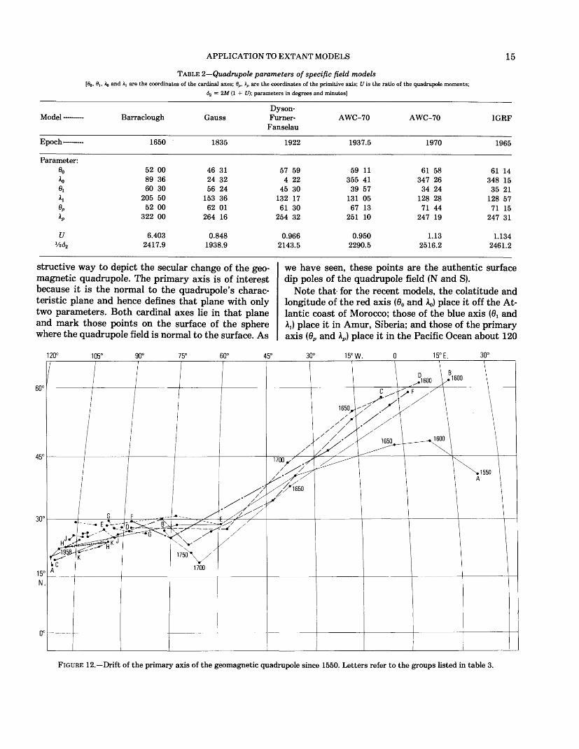
FIGURE 13.—Drift of the primary axis of the geomagnetic quadrupole since 1927. Letters refer to groups listed in table 3.
km from the extremity of Baja California. The three axes are, of course, orthogonal. Comparison of the Gauss model with recent ones shows clearly that all three axes have undergone a pronounced westward change of longitude, along with latitude changes sig nifying that the axis of rotation of the quadrupole is by no means coincident with the geographic axis. The 1650 model likewise supports this trend, at least qualitatively.
The Dyson-Furner-Fanselau parameters in table 2 agree well with the treatment by Howe (1939), which gives for that model the coordinates of the primary axis and of the cardinal axes. Most other published discussions of the quadrupole field lay chief stress on the primitive lines, and some go so far as to impute to their locations on the sphere the character of surface poles; but this concept is denied by the geometry as shown here.
30° 15°W.
APPLICATION TO EXTANT MODELS
15°E. 30° 45° 60° 75°
1790° 105° 120°
0°
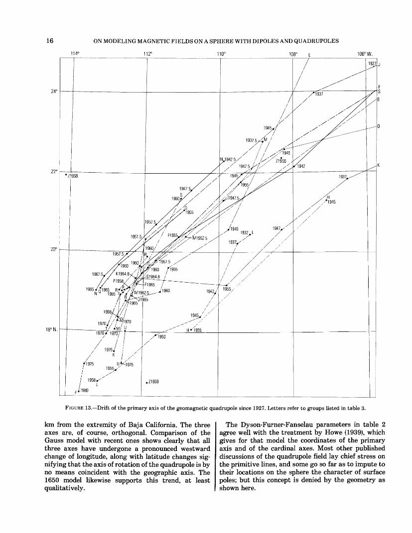
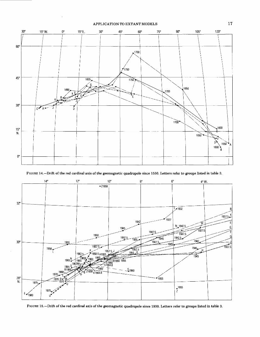
FIGURE 14.—Drift of the red cardinal axis of the geomagnetic quadrupole since 1550. Letters refer to groups listed in table 3.
14° 12° 10° 8° 6° 4°W.
FIGURE 15.—Drift of the red cardinal axis of the geomagnetic quadrupole since 1930. Letters refer to groups listed in table 3.
1890°
ON MODELING MAGNETIC FIELDS ON A SPHERE WITH DIPOLES AND QUADRUPOLES
105° E. 120° 135° 150° 165° 180° 195° 210° 225° 240° E.
0°
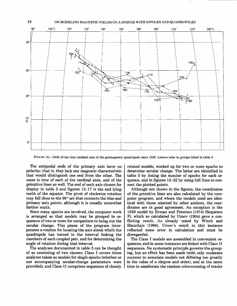
FIGURE 16.—Drift of the blue cardinal axis of the geomagnetic quadrupole since 1550. Letters refer to groups listed in table 3.
The antipodal ends of the primary axis have no polarity; that is, they lack any magnetic characteristic that would distinguish one end from the other. The same is true of each of the cardinal axes, and of the primitive lines as well. The end of each axis chosen for display in table 2 and figures 12-17 is the end lying north of the equator. The pivot of clockwise rotation may fall close to the 90 ° arc that connects the blue and primary axis points, although it is usually somewhat farther south.
Since many epochs are involved, the computer work is arranged so that models may be grouped in se quences of two or more for comparison to bring out the secular change. This phase of the program incor porates a routine for locating the axis about which the quadrupole has turned in the interval linking the members of each coupled pair, and for determining the angle of rotation during that interval.
The analyses documented in table 3 can be thought of as consisting of two classes: Class I covers those analyses taken as models for single epochs (whether or not accompanying secular-change parameters were provided); and Class II comprises sequences of closely
related models, worked up for two or more epochs to determine secular change. The latter are identified in table 3 by listing the number of epochs for each se quence, and in figures 12-22 by using full lines to con nect the plotted points.
Although not shown in the figures, the coordinates of the primitive lines are also calculated by the com puter program, and where the models used are iden tical with those selected by other authors, the coor dinates are in good agreement. An exception is the 1829 model by Erman and Petersen (1874) (Sequence F), which as calculated by Umov (1904) gave a con flicting result. As already noted by Winch and Slaucitajs (1966), Umov's result in this instance reflected some error in calculation and must be disregarded.
The Class I models are assembled in convenient se quences, and in some instances are linked with Class II sequences. No systematic principle governs the group ing, but an effort has been made (with only moderate success) to associate models not differing too greatly in the value of n (degree and order), and at the same time to ameliorate the random criss-crossing of tracks
52
128°E
APPLICATION TO EXTANT MODELS
130° 132° 134°
19
50°N
136°
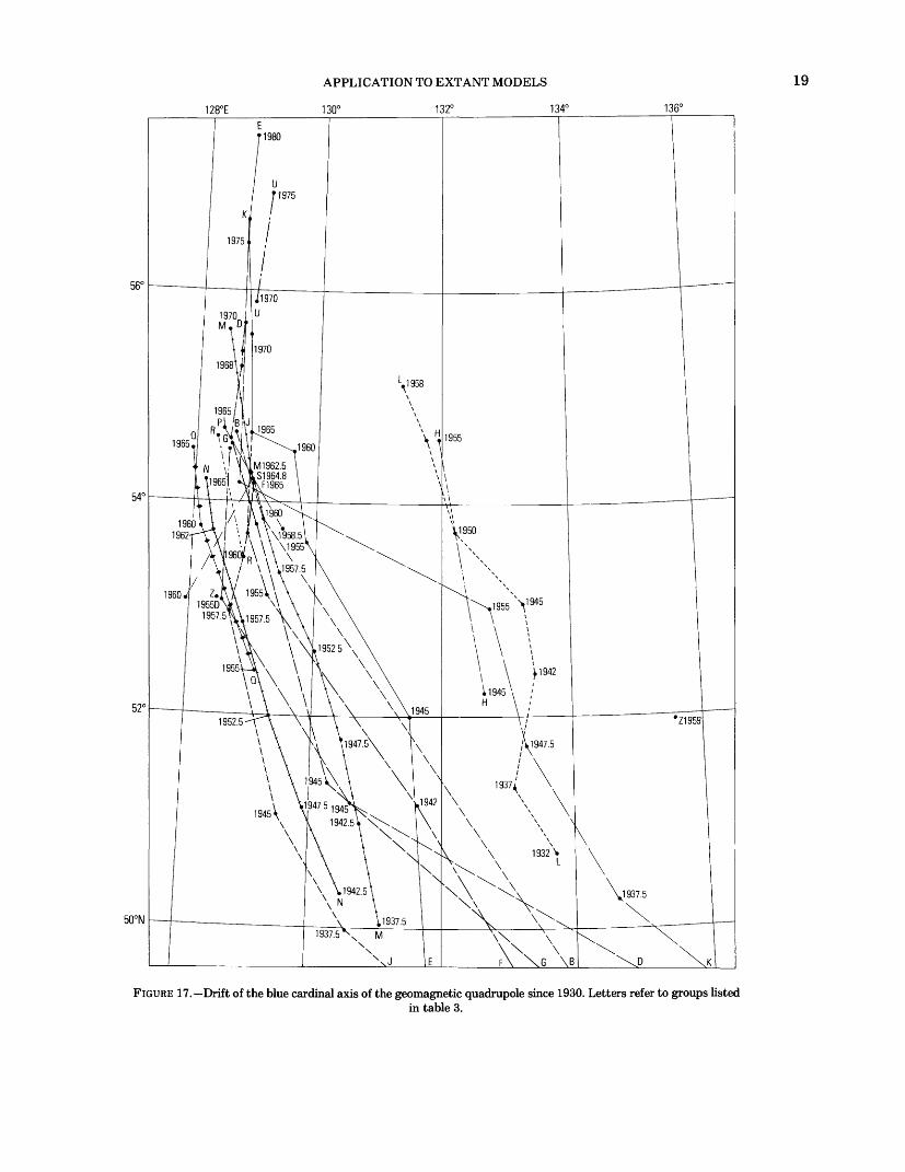
FIGURE 17.—Drift of the blue cardinal axis of the geomagnetic quadrupole since 1930. Letters refer to groups listedin table 3.
ON MODELING MAGNETIC FIELDS ON A SPHERE WITH DIPOLES AND QUADRUPOLES
1500 1600 1700 1800 1900 2000YEARS
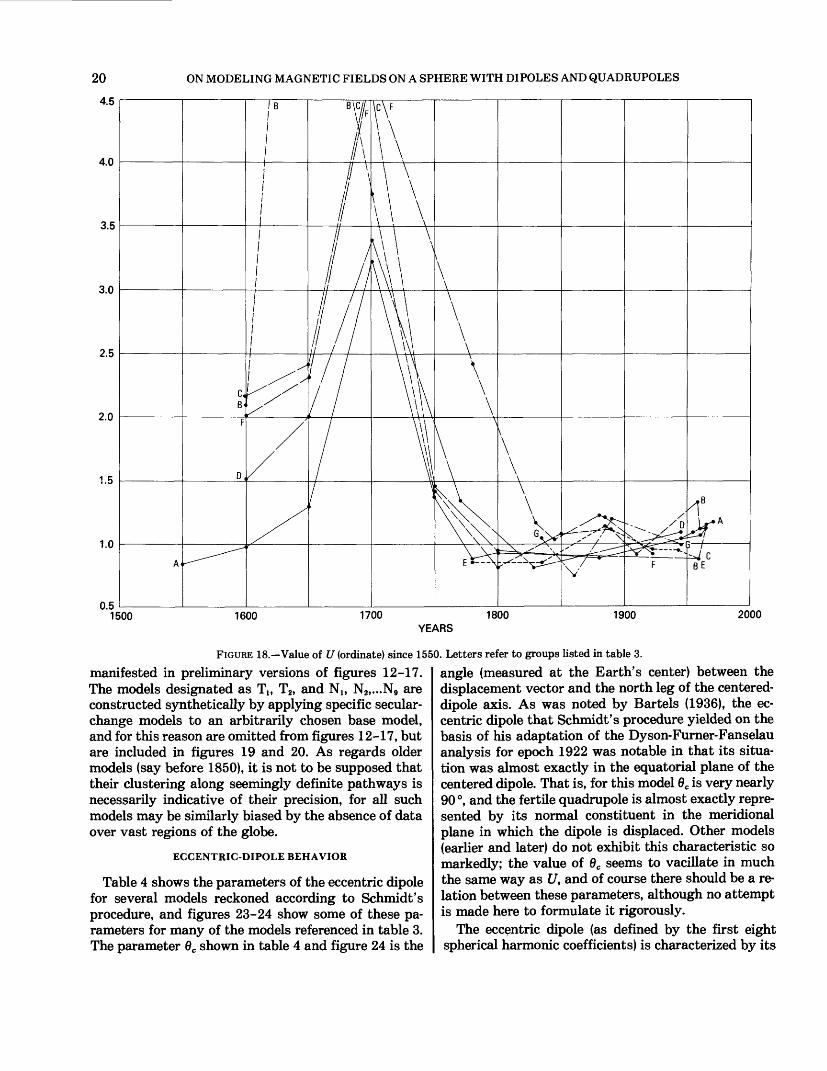
FIGURE 18.—Value of U (ordinate) since 1550. Letters refer to groups listed in table 3.manifested in preliminary versions of figures 12-17. The models designated as Ttt T2, and Nlt N2,...N9 are constructed synthetically by applying specific secular- change models to an arbitrarily chosen base model, and for this reason are omitted from figures 12-17, but are included in figures 19 and 20. As regards older models (say before 1850), it is not to be supposed that their clustering along seemingly definite pathways is necessarily indicative of their precision, for all such models may be similarly biased by the absence of data over vast regions of the globe.
ECCENTRIC-DIPOLE BEHAVIOR
Table 4 shows the parameters of the eccentric dipole for several models reckoned according to Schmidt's procedure, and figures 23-24 show some of these pa rameters for many of the models referenced in table 3. The parameter 6C shown in table 4 and figure 24 is the
angle (measured at the Earth's center) between the displacement vector and the north leg of the centered- dipole axis. As was noted by Bartels (1936), the ec centric dipole that Schmidt's procedure yielded on the basis of his adaptation of the Dyson-Furner-Fanselau analysis for epoch 1922 was notable in that its situa tion was almost exactly in the equatorial plane of the centered dipole. That is, for this model 6C is very nearly 90°, and the fertile quadrupole is almost exactly repre sented by its normal constituent in the meridional plane in which the dipole is displaced. Other models (earlier and later) do not exhibit this characteristic so markedly; the value of 6C seems to vacillate in much the same way as U, and of course there should be a re lation between these parameters, although no attempt is made here to formulate it rigorously.
The eccentric dipole (as defined by the first eight spherical harmonic coefficients) is characterized by its

APPLICATION TO EXTANT MODELS 21
1.20
1.15
1.10
1.05
1.00
0.95
0.901930 1940 1950
YEARS1960 1970
FIGURE 19.—Value of U (ordinate) since 1925. Letters refer to groups listed in table 3.
strength, its attitude, and its position. The first two features (and likewise their secular changes) are iden tical to those for the centered dipole. The third—that is, the vector stipulating how the dipole is displaced from the center of the sphere—is all that distinguishes the eccentric dipole from the centered one. This dis placement vector does exhibit significant secular changes or drifts, not only a westward drift but also a northward shifting; this was pointed out by Nagata (1965) and is confirmed in figure 23 for the past 8 or 10 decades. Those drifts in fact reflect changes in the strength and attitude of the quadrupole relative to the centered dipole. Hence it may be preferable to examine directly the quadrupole's changes so that its influence can be seen separately, uncontaminated by any "noise" or spurious constituents that might stem from uncertainties of the centered dipole.
For most of the models listed in table 3, the centered- dipole axis (south-seeking end) falls within the shaded area of figure 25; the exceptions are shown individually in the figure, and all relate to older models based on sparse data.
For an interesting treatment of multipole character istics relative to centered-dipole parameters, see Jory
(1956); his "sectorial quadrupole" appears to be what has been designated here as the sterile quadrupole.
RESULTS OF CALCULATIONS
The behavior brought out in figures 12-17 confirms the conclusions of Bullard and others (1950) and of other studies that the quadrupole is currently under going a pronounced drift. It may be called "westward" in the loose sense that the pivot or pole of clockwise ro tation is certainly in the Northern Hemisphere; but since that pole lies far from the geographic pole, the drift is not "westward" in the strictest sense. (In the Chukchi Sea, for example, the drift is roughly east ward.)
Figures 12-24 are offered to illustrate the capabili ties of the technique rather than to portray the exact quadrupole parameters. Any significance attached to the diagrams resides in the plotted points. The lines linking them in sequences should be regarded primar ily as identification aids, not as attempts to depict precise drift paths, particularly when the time span is more than 5 or 10 years. Some of the major discrepan cies manifested in figures 12-17 involve models that are derived wholly or chiefly from observatory data.
221.30
ON MODELING MAGNETIC FIELDS ON A SPHERE WITH DIPOLES AND QUADRUPOLES
1.20
R,,
1.10
\^*N,
1.00
0.901910 1920 1930 1940 1950 1960 1970
YEARS
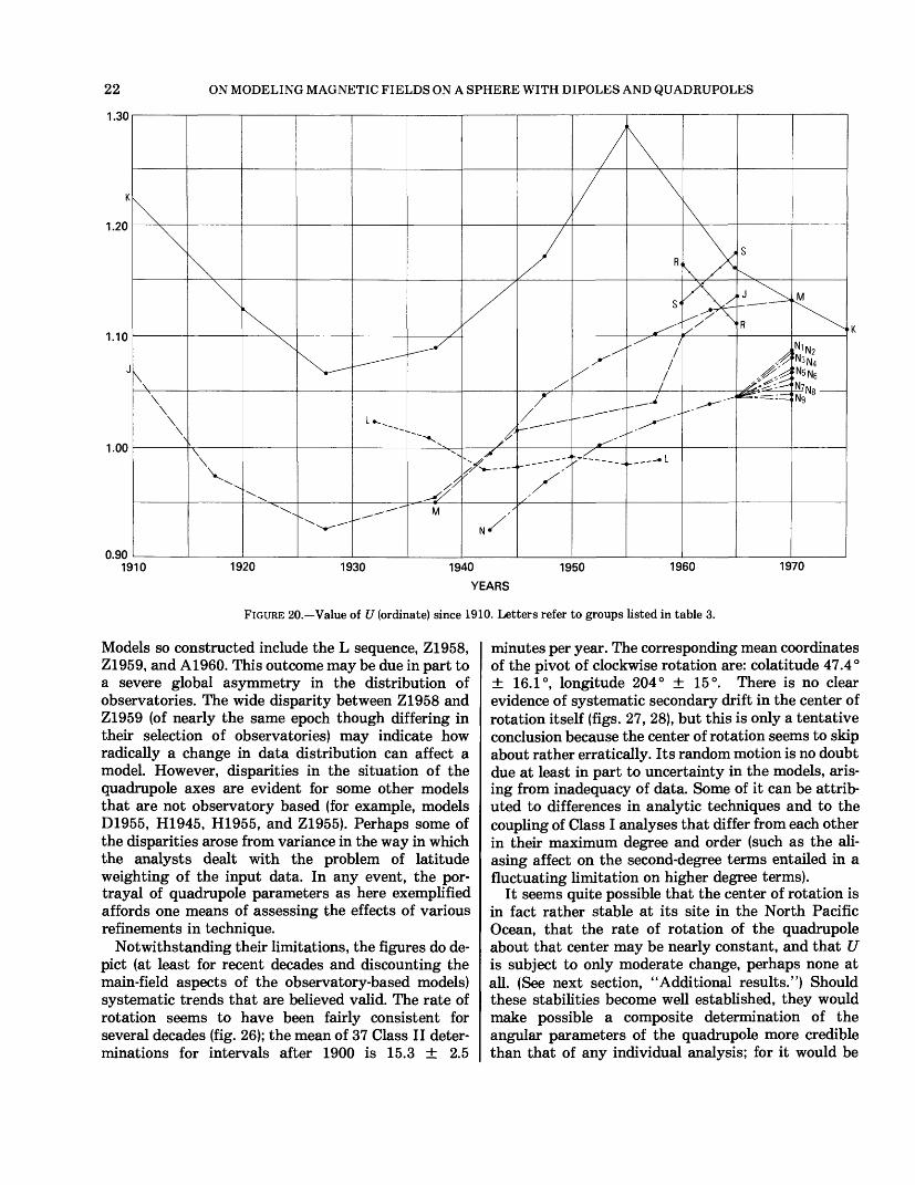
FIGURE 20.—Value of U (ordinate) since 1910. Letters refer to groups listed in table 3.
Models so constructed include the L sequence, Z1958, Z1959, and A1960. This outcome may be due in part to a severe global asymmetry in the distribution of observatories. The wide disparity between Z1958 and Z1959 (of nearly the same epoch though differing in their selection of observatories) may indicate how radically a change in data distribution can affect a model. However, disparities in the situation of the quadrupole axes are evident for some other models that are not observatory based (for example, models D1955, H1945, H1955, and Z1955). Perhaps some of the disparities arose from variance in the way in which the analysts dealt with the problem of latitude weighting of the input data. In any event, the por trayal of quadrupole parameters as here exemplified affords one means of assessing the effects of various refinements in technique.
Notwithstanding their limitations, the figures do de pict (at least for recent decades and discounting the main-field aspects of the observatory-based models) systematic trends that are believed valid. The rate of rotation seems to have been fairly consistent for several decades (fig. 26); the mean of 37 Class II deter minations for intervals after 1900 is 15.3 ± 2.5
minutes per year. The corresponding mean coordinates of the pivot of clockwise rotation are: colatitude 47.4° ± 16.1°, longitude 204° ±15°. There is no clear evidence of systematic secondary drift in the center of rotation itself (figs. 27, 28), but this is only a tentative conclusion because the center of rotation seems to skip about rather erratically. Its random motion is no doubt due at least in part to uncertainty in the models, aris ing from inadequacy of data. Some of it can be attrib uted to differences in analytic techniques and to the coupling of Class I analyses that differ from each other in their maximum degree and order (such as the ali asing affect on the second-degree terms entailed in a fluctuating limitation on higher degree terms).
It seems quite possible that the center of rotation is in fact rather stable at its site in the North Pacific Ocean, that the rate of rotation of the quadrupole about that center may be nearly constant, and that U is subject to only moderate change, perhaps none at all. (See next section, "Additional results.") Should these stabilities become well established, they would make possible a composite determination of the angular parameters of the quadrupole more credible than that of any individual analysis; for it would be
APPLICATION TO EXTANT MODELS 23
'E
J*"//
161800, 1820 1840 1860 1880 1900
YEARS1920 1940 1960 1980
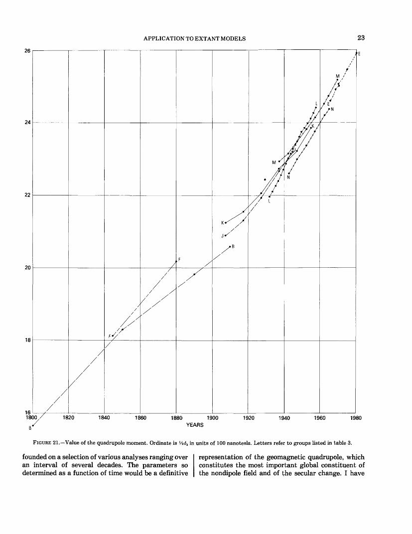
FIGURE 21.—Value of the quadrupole moment. Ordinate is 1A62 in units of 100 nanotesla. Letters refer to groups listed in table 3.
founded on a selection of various analyses ranging over an interval of several decades. The parameters so determined as a function of time would be a definitive
representation of the geomagnetic quadrupole, which constitutes the most important global constituent of the nondipole field and of the secular change. I have

ON MODELING MAGNETIC FIELDS ON A SPHERE WITH DIPOLES AND QUADRUPOLES
-op
1.0\K \
1800 1820 1840 1860 1880 1900 YEARS
1920 1940 1960 1980
FIGURE 22.—Change of the quadrupole moment over time (sheared plot). In rectangular coordinates, the graph depicts the ordinate as( l/262 + 94.2 — 0.06 X year). Letters refer to groups listed in table 3.
refrained from attempting such a determination; in view of the diverse provenance of the constituent models and the possible impact of the results upon future modeling efforts, it is felt that a joint under taking by various agencies and individuals concerned would be more authoritative than any unilateral effort.
If future analyses with more evenly distributed data show that the pivot of rotation holds its position better than do the quadrupole axes, this finding will enhance the significance of the quadrupole and afford further testimony as to its conservative tendency.
The fact that the pivot of rotation is clearly far from the geographic pole lends support to a similar finding by Malin and Saunders (1973) with respect to the ro tation of the composite of multipole fields up to degree six. The further fact that the latter's pole of rotation as reported by those authors differs radically from that for the quadrupole alone as found here tends likewise to support their suggestion that the higher degree multipoles are important in establishing the secular drift of the field as a whole.
Figure 21 shows, for some of the Class II models, the changes in the combined quadrupole moment, which is the numerical sum of the red and blue linear com ponents marking the cardinal axes, and is denoted in equation (12) and in table 2 as 1A62 . These changes are
fairly steady at about 0.3 percent per year, as previ ously reported by Winch and Slaucitajs (1966). This graph is drawn to exclude results earlier than 1800, be cause such early values are necessarily conjectural for lack of pertinent intensity data.
The quantity actually given in table 2 and figure 21 is yz62 , expressed in nanoteslas (nT) for convenient comparison. To convert into quadrupole moment (unit, weber-km2 ), multiply by 1.6477 X 10 15 . The data shown in figure 21 are replotted in figure 22 on a sheared basis—that is, with a fixed linear slope of +0.06 nT per year subtracted from each value before plotting, thus permitting an expanded ordinate scale and clarifying the relation of the different sequences. The absolute value for any plotted point may be recovered by scaling vertically from the inclined grid lines.
The several parameters of the quadrupole have been worked up as a demonstration of technique and a step in advancing the understanding of the nondipole field and its secular change. It remains to be seen to what extent analogous procedures and spatial concepts may apply to the octupole and higher multipoles. Mean while, the situation of the quadrupole is well estab lished, with its primary axis emerging in the Revilla Gigodo Islands off the Gulf of California, its red and blue axes respectively between southern Morocco and
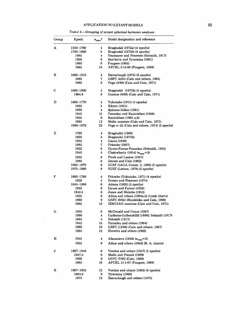
APPLICATION TO EXTANT MODELS 25
TABLE 3.—Grouping of extant spherical harmonic analyses
Group
A
B
C
D
E
F
G
H
J
K
Epoch
1550-17001750-1800
1885195819601965
1600-191019601965
1600-18001964.8
1600-177018301880194519551965
1968-1970
17801800183518851922194519551960
1965-19701975-1980
1600-17801829
1845-18801922
1942.5195519601965
183518601885194519601965
19451955
1907-19451957.519601965
1907-19551964.81975
"rnaxt
45468
10
479
49
454
156
1222
4547646688
4466669
10
644
151012
46
669
10
129
12
Model designation and reference
Braginskii (1972a) (4 epochs)Braginskii (1972b) (3 epochs)Neumayer and Petersen (Schmidt, 1917)Ben'kova and Tyurmina (1961)Fougere (1965)AFCRL 3-15-68 (Fougere, 1969)
Barraclough (1974) (8 epochs)GSFC (4/64) (Cain and others, 1965)Pogo (3/68) (Cain and Cain, 1971)
Braginskii (1972b) (5 epochs)Cosmos (9/68) (Cain and Cain, 1971)
Yukutake (1971) (4 epochs)Kamtz (1851)Quintus-Icilius (1881)Fanselau and Kautzleben (1958)Kautzleben (1965 a,b)Malin nominee (Cain and Cain, 1971)Pogo n-22 (Cain and others, 1974) (2 epochs)
Braginskii (1969)Braginskii (1972b)Gauss (1839)Fritsche (1897)Dyson-Furner-Fanselau (Schmidt, 1934)Chakrabarty (1954) (ramax=2)Finch and Leaton (1957)Jensen and Cain (1962)IGRF (IAGA Comm. 2, 1969) (2 epochs)IGRF (Leaton, 1976) (2 epochs)
Fritsche (Yukutake, 1971) (4 epochs)Erman and Petersen (1874)Adams (1900) (2 epochs)Dyson and Furner (1923)Jones and Melotte (1953)Adam and others (1963a,b) (Izmir charts)GSFC (9/65) (Hendricks and Cain, 1966)IZMIRAN nominee (Cain and Cain, 1971)
McDonald and Gunst (1967)Carlheim-Gyllenskb'ld (1896); Schmidt (1917)Schmidt (1917)Fanselau and others (1964)GSFC (12/66) (Cain and others, 1967)Hurwitz and others (1966)
Afanasieva (1946) (nmax=2)Adam and others (1962) (B. A. charts)
Vestine and others (1947) (5 epochs)Malin and Pocock (1969)GSFC (7/65) (Cain, 1966)AFCRL 11-1-67 (Fougere, 1969)
Vestine and others (1963) (6 epochs)Tyurmina (1968)Barraclough and others (1975)
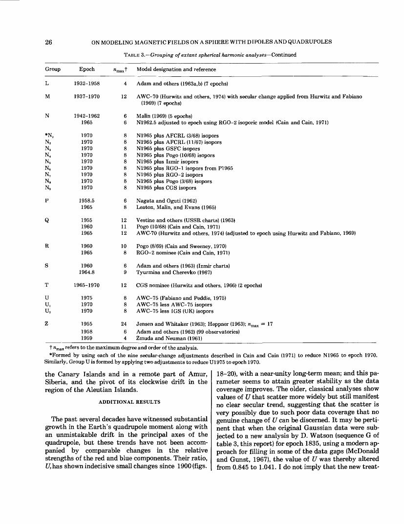
26 ON MODELING MAGNETIC FIELDS ON A SPHERE WITH DIPOLES AND QUADRUPOLES
TABLE 3.— Grouping of extant spherical harmonic analyses—Continued
Group Epoch Model designation and reference
L 1932-1958 4 Adam and others (1963a,b) (7 epochs)
M 1937-1970 12 AWC-70 (Hurwitz and others, 1974) with secular change applied from Hurwitz and Fabiano(1969) (7 epochs)
N 1942-1962 6 Malin (1969) (5 epochs)1965 6 N1962.5 adjusted to epoch using RGO-2 isoporic model (Cain and Cain, 1971)
*N, 1970 8 N1965 plus AFCRL (3/68) isoporsN2 1970 8 N1965 plus AFCRL (11/67) isoporsN3 1970 8 N1965 plus GSFC isoporsN4 1970 8 N1965 plus Pogo (10/68) isoporsN5 1970 8 N1965 plus Izmir isoporsN6 1970 8 N1965 plus RGO-1 isopors from P1965N7 1970 8 N1965 plus RGO-2 isoporsN8 1970 8 N1965 plus Pogo (3/68) isoporsN9 1970 8 N1965 plus CGS isopors
P 1958.5 6 Nagata and Oguti (1962)1965 8 Leaton, Malin, and Evans (1965)
Q 1955 12 Vestine and others (USSR charts) (1963)1960 11 Pogo (10/68) (Cain and Cain, 1971)1965 12 AWC-70 (Hurwitz and others, 1974) (adjusted to epoch using Hurwitz and Fabiano, 1969)
R 1960 10 Pogo (8/69) (Cain and Sweeney, 1970)1965 8 RGO-2 nominee (Cain and Cain, 1971)
S 1960 6 Adam and others (1963) (Izmir charts)1964.8 9 Tyurmina and Cherevko (1967)
T 1965-1970 12 CGS nominee (Hurwitz and others, 1966) (2 epochs)
U 1975 8 AWC-75 (Fabiano and Peddie, 1975)U, 1970 8 AWC-75 less AWC-75 isoporsU2 1970 8 AWC-75 less IGS (UK) isopors
Z 1955 24 Jensen and Whitaker (1963); Heppner (1963); ramax = 171958 6 Adam and others (1962) (99 observatories)
_________1959_______4 Zmuda and Neuman (1961) ______________________________t "max refers to the maximum degree and order of the analysis.*Formed by using each of the nine secular-change adjustments described in Cain and Cain (1971) to reduce N1965 to epoch 1970.
Similarly, Group U is formed by applying two adjustments to reduce U1975 to epoch 1970.
the Canary Islands and in a remote part of Amur, Siberia, and the pivot of its clockwise drift in the region of the Aleutian Islands.
ADDITIONAL RESULTS
The past several decades have witnessed substantial growth in the Earth's quadrupole moment along with an unmistakable drift in the principal axes of the quadrupole, but these trends have not been accom panied by comparable changes in the relative strengths of the red and blue components. Their ratio, C/,has shown indecisive small changes since 1900 (figs.
18-20), with a near-unity long-term mean; and this pa rameter seems to attain greater stability as the data coverage improves. The older, classical analyses show values of U that scatter more widely but still manifest no clear secular trend, suggesting that the scatter is very possibly due to such poor data coverage that no genuine change of U can be discerned. It may be perti nent that when the original Gaussian data were sub jected to a new analysis by D. Watson (sequence G of table 3, this report) for epoch 1835, using a modern ap proach for filling in some of the data gaps (McDonald and Gunst, 1967), the value of U was thereby altered from 0.845 to 1.041. I do not imply that the new treat-
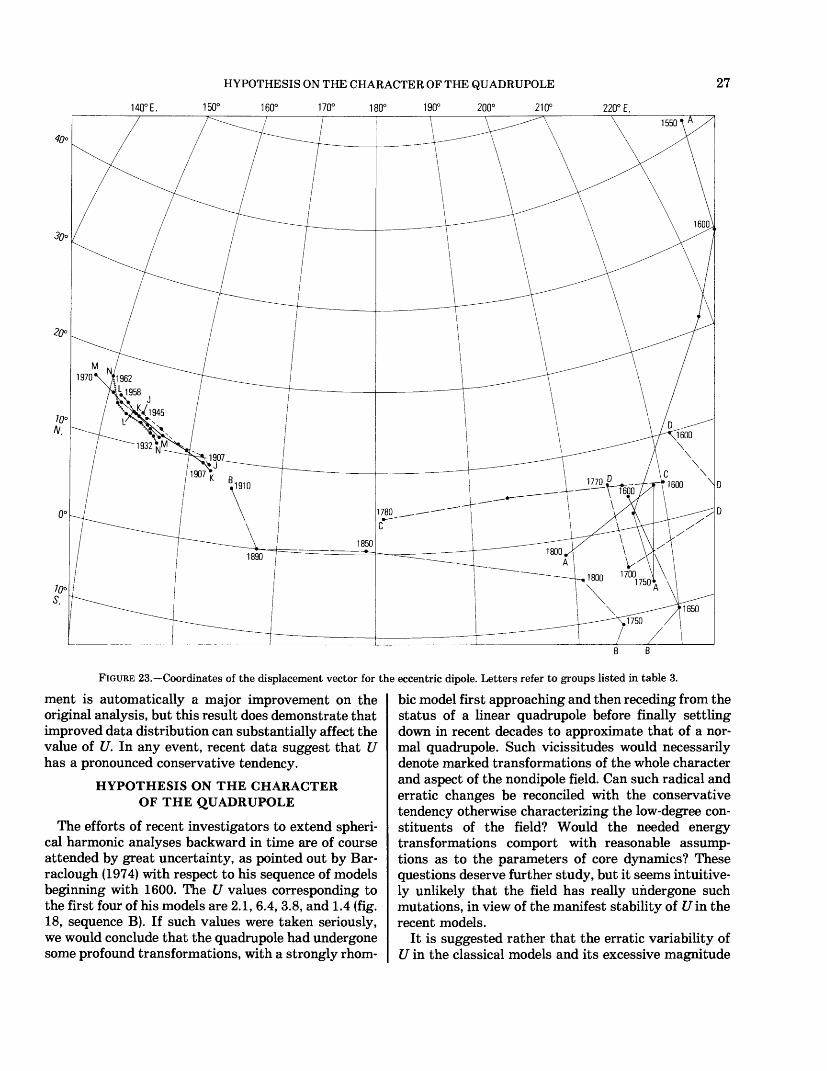
140° E.
HYPOTHESIS ON THE CHARACTER OF THE QUADRUPOLE
150° 160° 170° 180° 190° 200° 210°
27
220° E.
FIGURE 23.—Coordinates of the displacement vector for the eccentric dipole. Letters refer to groups listed in table 3.
ment is automatically a major improvement on the original analysis, but this result does demonstrate that improved data distribution can substantially affect the value of U. In any event, recent data suggest that U has a pronounced conservative tendency.
HYPOTHESIS ON THE CHARACTER OF THE QUADRUPOLE
The efforts of recent investigators to extend spheri cal harmonic analyses backward in time are of course attended by great uncertainty, as pointed out by Bar- raclough (1974) with respect to his sequence of models beginning with 1600. The U values corresponding to the first four of his models are 2.1, 6.4, 3.8, and 1.4 (fig. 18, sequence B). If such values were taken seriously, we would conclude that the quadrupole had undergone some profound transformations, with a strongly rhom
bic model first approaching and then receding from the status of a linear quadrupole before finally settling down in recent decades to approximate that of a nor mal quadrupole. Such vicissitudes would necessarily denote marked transformations of the whole character and aspect of the nondipole field. Can such radical and erratic changes be reconciled with the conservative tendency otherwise characterizing the low-degree con stituents of the field? Would the needed energy transformations comport with reasonable assump tions as to the parameters of core dynamics? These questions deserve further study, but it seems intuitive ly unlikely that the field has really undergone such mutations, in view of the manifest stability of U in the recent models.
It is suggested rather that the erratic variability of U in the classical models and its excessive magnitude
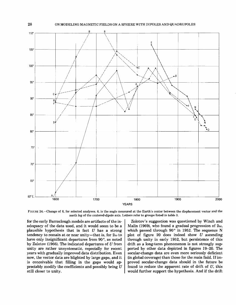
28
110°
ON MODELING MAGNETIC FIELDS ON A SPHERE WITH DIPOLES AND QUADRUPOLES
B B
60° E.1600 1700 1800 1900 2000
YEARS
FIGURE 24.—Change of Bc for selected analyses. 0C is the angle measured at the Earth's center between the displacement vector and thenorth leg of the centered-dipole axis. Letters refer to groups listed in table 3.
for the early Barraclough models are artifacts of the in adequacy of the data used, and it would seem to be a plausible hypothesis that in fact U has a strong tendency to remain at or near unity—that is, for 2co to have only insignificant departures from 90 °, as noted by Zolotov (1966). The indicated departures of U from unity are rather unsystematic, especially for recent years with gradually improved data distribution. Even now, the vector data are blighted by large gaps, and it is conceivable that filling in the gaps would ap preciably modify the coefficients and possibly bring U still closer to unity.
Zolotov's suggestion was questioned by Winch and Malin (1969), who found a gradual progression of 2o>, which passed through 90° in 1952. The sequence N plot of figure 20 does indeed show U ascending through unity in early 1952, but persistence of this drift as a long-term phenomenon is not strongly sup ported by other data depicted in figures 19-20. The secular-change data are even more seriously deficient (in global coverage) than those for the main field. If im proved secular-change data should in the future be found to reduce the apparent rate of drift of U, this would further support the hypothesis. And if the drift

SOME FURTHER IMPLICATIONS OF THE QUADRUPOLE CONSTRAINT 29
TABLE 4—Eccentric-dipole parameters of specific field models[Of the two versions of the displacement-vector parameters, those on the lower h'ne of each pair are modified values obtained by imposing the constraint for U = 1, holding the
cardinal axes unchanged. Rc, magnitude of the displacement vector in terms of Earth radii. 6C, angle measured at the Earth's center between the displacement vector and the north leg of the centered-dipole axis. Angles in degrees and minutes]
Model - —— —
Epoch ——— -
Dipole vector:eA
Displacement vector:
ec
AC
6C
Rc
Barraclough
1650
7 16 319 09
100 31 97 33
210 01 239 51
102 51 96 09
0.05164 0.03267
Gauss
1835
12 10 296 28
103 06 103 01
185 24 185 24
106 36 107 06
0.04540 0.04452
Dyson- Furner-
Fanselau
1922
11 30 291 10
83 28 83 25
161 44 161 08
90 50 90 52
0.05397 0.05395
AWC-70
1937.5
11 30 291 57
78 36 78 25
156 22 155 37
86 53 86 49
0.06240 0.06242
AWC-70
1970
11 26289 47
71 27 72 01
148 02 149 39
80 32 80 54
0.07270 0.07224
IGRF
1965
11 26 290 14
72 50 73 24
148 46 150 25
81 53 82 15
0.07067 0.07025
is real, it may change sign from time to time so that U never gets far from unity.
Different attempts to derive isoporic models yield discordant rates of change of U, despite the use of re cent data and updated techniques. Nine proposals were formally entered in 1968 as candidates for the time derivative terms of the International Geomagnetic Reference Field. Their second-degree terms are reflected in the cluster of nine short lines in figure 20 for the interval 1965-1970. No doubt the slope dispari ty stems partly from differences in the weighting of data; if the well-known global imbalance of obser vatory distribution could be remedied, such a spread might well be minimized. (Note that the attachment of this grouping to a particular main-field model is ar bitrary and holds no significance as to the absolute value of U.)
If the hypothesis that U is constrained to remain at or close to unity is tenable, then many of the older models, if not the current ones, could be improved by imposing the empirical constraint that U = 1 . Geometrically, this constraint implies that the zonal element delimited by any two small circles parallel to the characteristic plane of the quadrupole and by "meridians" of the primary axis that are 180° apart will encompass zero net quadrupole flux (the total amounts that enter and leave that part of the sphere being equal). The hypothesis, then, in its boldest form asserts that the configuration of the several electric-
current vortices comprising the nondipole part of the geomagnetic core-dynamo is in some way physically regularized so that it cannot give rise to a quadrupole that differs significantly from a normal one.
SOME FURTHER IMPLICATIONS OF THE QUADRUPOLE CONSTRAINT
It is pertinent to inquire whether the hypothesis has any physical basis. None of a rigorous character ap pears, but a limited facet of the matter is to be noted. Let us regard a quadrupole as the result of two nearby current loops (of contrary sense) in a plasma, depicting two dipoles. Their detailed interplay, rather than their gross equivalence to simple dipoles, will govern the outcome.
For a normal quadrupole the loops would be coplanar, and their affinity would lead to an equilibrium configuration (fig. 29A), wherein the at traction between uncrossed remnants of the inner limbs is balanced by that between the overlapping seg ments (now urging the loops apart) plus the net repul sion involving the outer limbs. If the loops are con sidered to merge in their shared region (fig. 29B), the forces change but the equilibrium spacing is much the same. For a linear quadrupole the loops must be coax ial, one over the other, rather than coplanar. In this case (irrespective of the separation) there is no net attraction but only repulsion, precluding any
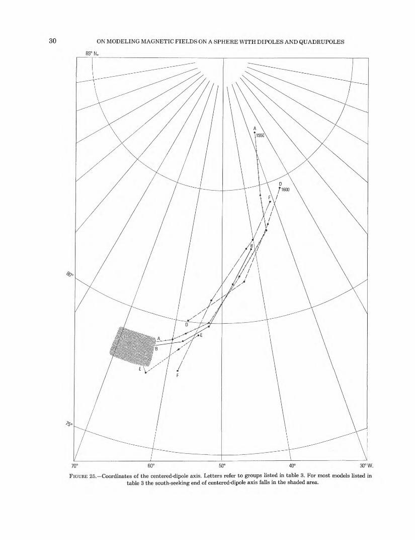
30 ON MODELING MAGNETIC FIELDS ON A SPHERE WITH DIPOLES AND QUADRUPOLES
85° N.
60° 50° 40° 30° W.
FIGURE 25.—Coordinates of the centered-dipole axis. Letters refer to groups listed in table 3. For most models listed in table 3 the south-seeking end of centered-dipole axis falls in the shaded area.
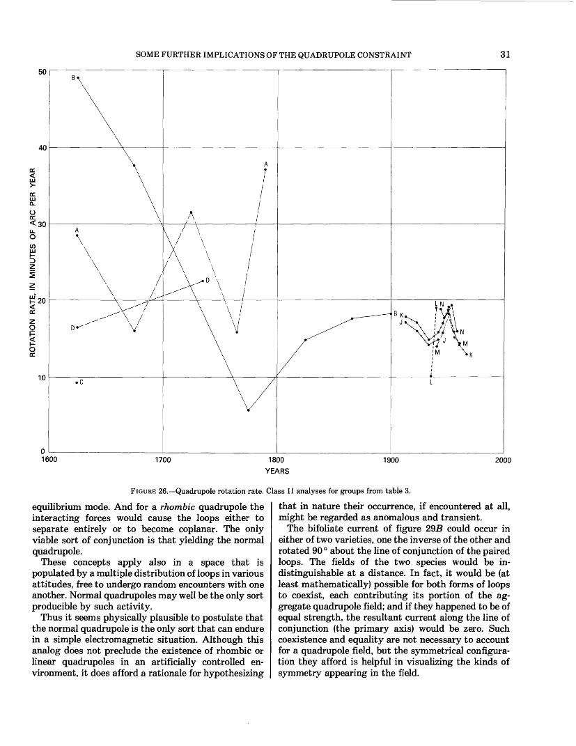
SOME FURTHER IMPLICATIONS OF THE QUADRUPOLE CONSTRAINT 31
50
40
DC LLJ Q.
ODC<30u.O
I
\
20
D""' V
10
1600 1700 1800 YEARS
1900 2000
FIGURE 26.—Quadrupole rotation rate. Class II analyses for groups from table 3.
equilibrium mode. And for a rhombic quadrupole the interacting forces would cause the loops either to separate entirely or to become coplanar. The only viable sort of conjunction is that yielding the normal quadrupole.
These concepts apply also in a space that is populated by a multiple distribution of loops in various attitudes, free to undergo random encounters with one another. Normal quadrupoles may well be the only sort producible by such activity.
Thus it seems physically plausible to postulate that the normal quadrupole is the only sort that can endure in a simple electromagnetic situation. Although this analog does not preclude the existence of rhombic or linear quadrupoles in an artificially controlled en vironment, it does afford a rationale for hypothesizing
that in nature their occurrence, if encountered at all, might be regarded as anomalous and transient.
The bifoliate current of figure 295 could occur in either of two varieties, one the inverse of the other and rotated 90° about the line of conjunction of the paired loops. The fields of the two species would be in distinguishable at a distance. In fact, it would be (at least mathematically) possible for both forms of loops to coexist, each contributing its portion of the ag gregate quadrupole field; and if they happened to be of equal strength, the resultant current along the line of conjunction (the primary axis) would be zero. Such coexistence and equality are not necessary to account for a quadrupole field, but the symmetrical configura tion they afford is helpful in visualizing the kinds of symmetry appearing in the field.
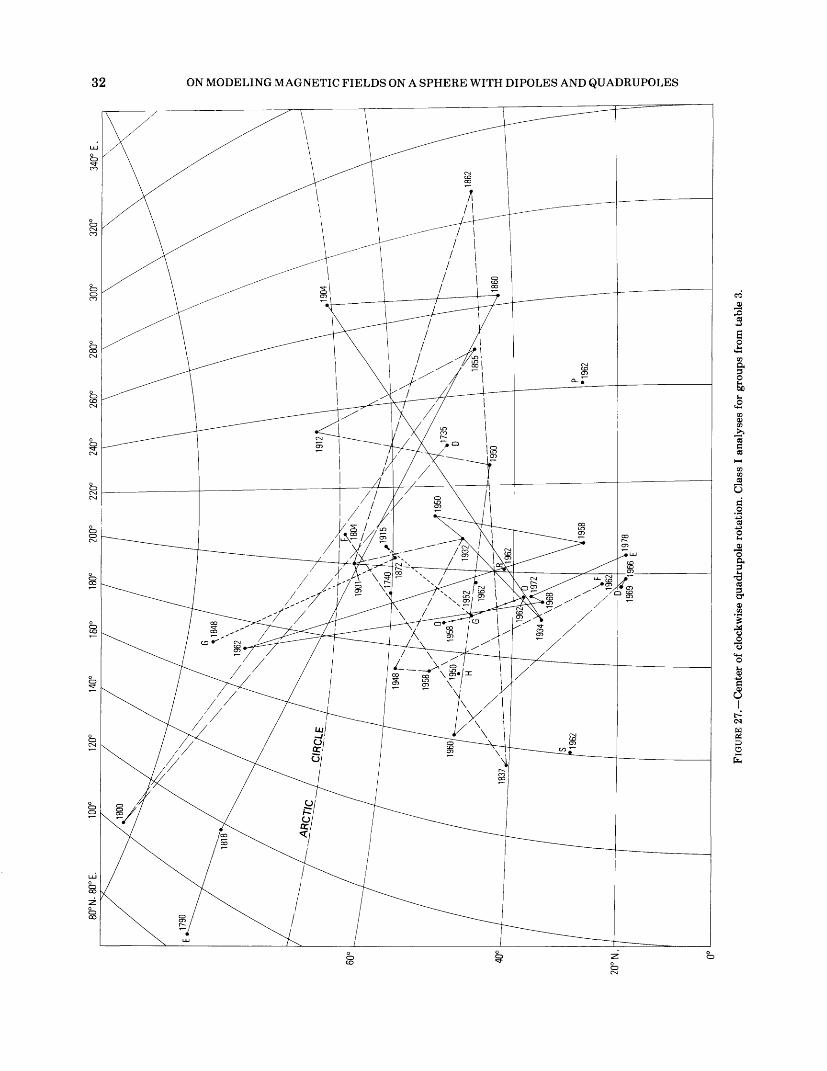
32 ON MODELING MAGNETIC FIELDS ON A SPHERE WITH DIPOLES AND QUADRUPOLES
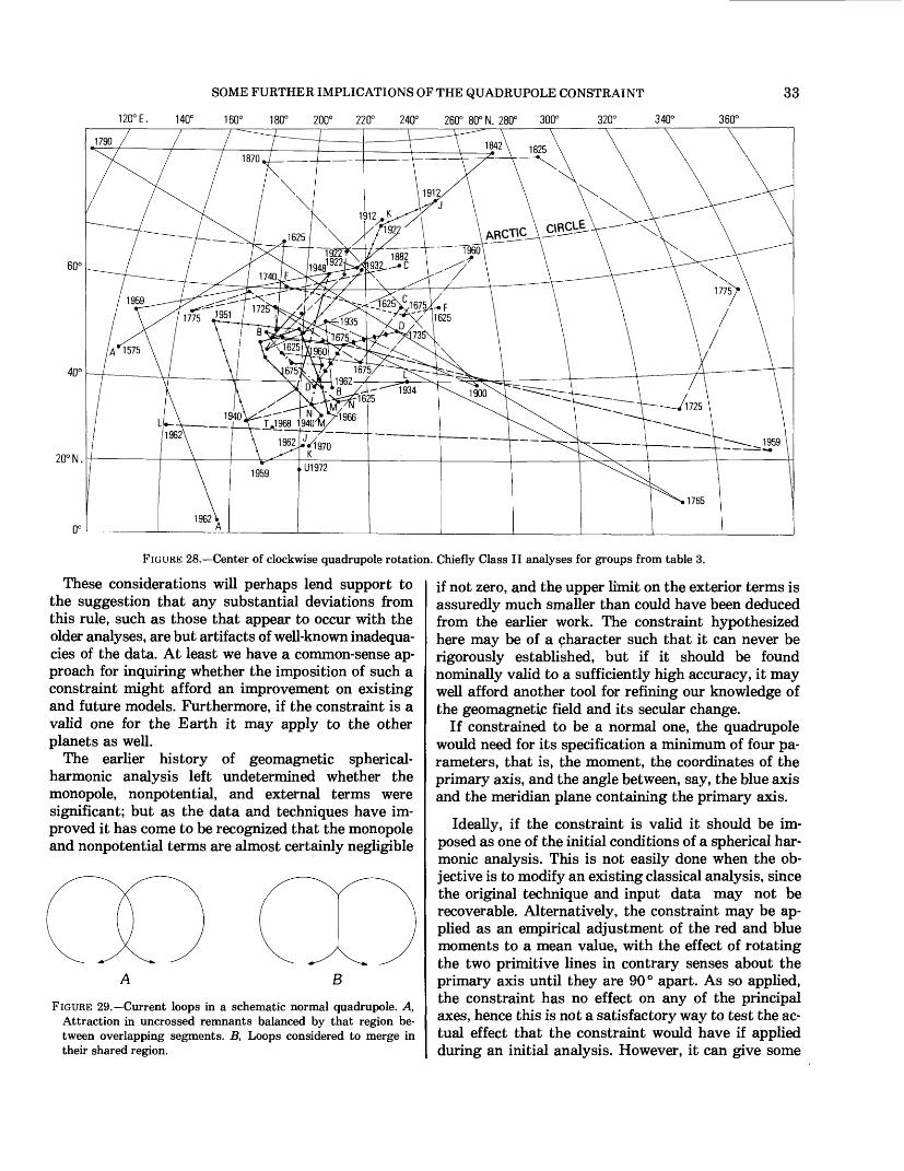
120°E. 140°
SOME FURTHER IMPLICATIONS OF THE QUADRUPOLE CONSTRAINT
160° 180° 200° 220° 240° 260° 80° N. 280° 300° 320° 340°
33360°
20° N.
0°
FIGURE 28.—Center of clockwise quadrupole rotation. Chiefly Class II analyses for groups from table 3.
These considerations will perhaps lend support to the suggestion that any substantial deviations from this rule, such as those that appear to occur with the older analyses, are but artifacts of well-known inadequa cies of the data. At least we have a common-sense ap proach for inquiring whether the imposition of such a constraint might afford an improvement on existing and future models. Furthermore, if the constraint is a valid one for the Earth it may apply to the other planets as well.
The earlier history of geomagnetic spherical- harmonic analysis left undetermined whether the monopole, nonpotential, and external terms were significant; but as the data and techniques have im proved it has come to be recognized that the monopole and nonpotential terms are almost certainly negligible
FIGURE 29.—Current loops in a schematic normal quadrupole. A, Attraction in uncrossed remnants balanced by that region be tween overlapping segments. B, Loops considered to merge in their shared region.
if not zero, and the upper limit on the exterior terms is assuredly much smaller than could have been deduced from the earlier work. The constraint hypothesized here may be of a 9haracter such that it can never be rigorously established, but if it should be found nominally valid to a sufficiently high accuracy, it may well afford another tool for refining our knowledge of the geomagnetic field and its secular change.
If constrained to be a normal one, the quadrupole would need for its specification a minimum of four pa rameters, that is, the moment, the coordinates of the primary axis, and the angle between, say, the blue axis and the meridian plane containing the primary axis.
Ideally, if the constraint is valid it should be im posed as one of the initial conditions of a spherical har monic analysis. This is not easily done when the ob jective is to modify an existing classical analysis, since the original technique and input data may not be recoverable. Alternatively, the constraint may be ap plied as an empirical adjustment of the red and blue moments to a mean value, with the effect of rotating the two primitive lines in contrary senses about the primary axis until they are 90° apart. As so applied, the constraint has no effect on any of the principal axes, hence this is not a satisfactory way to test the ac tual effect that the constraint would have if applied during an initial analysis. However, it can give some
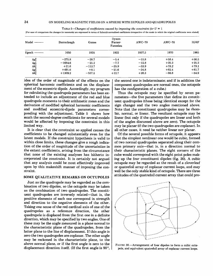
34 ON MODELING MAGNETIC FIELDS ON A SPHERE WITH DIPOLES AND QUADRUPOLES
TABLE 5—Changes of coefficients caused by imposing the constraint for U = 1[For ease of comparison the changes (in nanotesla) are expressed in terms of Schmidt-normalized coefficients irrespective of the mode in which the original coefficients were stated]
Model Barraclough GaussDyson- Furner-
FanselauAWC-70 AWC-70 IGRF
Epoch 1650 1835 1922 1937.5 1970 1965
Ag-£ -275.8Agi -1684.6Lh\ +21.6Ag| +491.6Lh\ +1309.2
-28.7-21.2
-113.7+8.1
-557.5
-5.4-7.7
-25.9-21.6+ 12.7
-15.8-12.8-33.9-34.8+26.3
+58.4+25.2+78.2+82.4-86.8
+56.5+25.2+ 79.1+81.7-84.9
idea of the order of magnitude of the effects on the spherical harmonic coefficients and on the displace ment of the eccentric dipole. Accordingly, my program for calculating the quadrupole parameters has been ex tended to include an adjustment of the red and blue quadrupole moments to their arithmetic mean and the derivation of modified spherical harmonic coefficients and modified eccentric-dipole parameters corres ponding with the adjustment. Table 5 shows how much the second-degree coefficients for several models would be affected by imposing the constraint in this limited way.
It is clear that the constraint so applied causes the coefficients to be changed substantially even for the latest models. If the constraint hypothesis is valid to within close limits, these changes give a rough indica tion of the order of magnitude of the uncertainties in the extant coefficients, arising from the circumstance that none of the existing analyses has hitherto in corporated the constraint. It is certainly not argued that any analysis could be most effectively improved upon by this makeshift manner of imposing the con straint.
SOME QUALITATIVE REMARKS ON OCTUPOLESJust as the quadrupole may be regarded as the com
bination of two dipoles, so the octupole may be taken as the combination of two quadrupoles. The constit uent quadrupoles are inversely related—that is, the positive elements of each one correspond in strength and direction to the negative elements of the other. Taking one sense of the red cardinal axis of one of the quadrupoles as a reference direction, the other quadrupole is displaced from the first one in a definite direction, which may be specified by two angles. One of these may be the angle measured in a plane normal to the characteristic plane of the quadrupoles, from the latter plane to the line of displacement. If this angle is zero the two quadrupoles are coplanar. The other angle may be reckoned in the characteristic plane, to the above normal plane, or if the first angle is zero to the displacement direction itself. (If the first angle is 90°,
the second one is indeterminate; and if in addition the component quadrupoles are normal ones, the octupole has the configuration of a cube.)
Thus the octupole may be specified by seven pa rameters—the five parameters that define its constit uent quadrupoles (these being identical except for the sign change) and the two angles mentioned above. Note that the constituent quadrupoles may be rhom bic, normal, or linear. The resultant octupole may be linear (but only if the quadrupoles are linear and both of the angles discussed above are zero). The octupole may be planar (if the two quadrupoles are coplanar). In all other cases, it need be neither linear nor planar.
Of the several possible forms of octupole, it appears that the simplest nonlinear one would be cubic, formed of two normal quadrupoles separated along their com mon primary axis—that is, in a direction normal to their characteristic planes. The eight corners of the cube would correspond with the eight point poles mak ing up the four constituent dipoles (fig. 30). A cubic octupole may be regarded as the result of a cloverleaf or quatrefoil array of coplanar current loops, and may well be the only stable kind of octupole. There are three attitudes of the quatrefoil current array that could pro-
FIGURE 30.—Arrangement of four dipoles to form a cubic octu pole, and equivalent quatrefoil array of coplanar current loops.
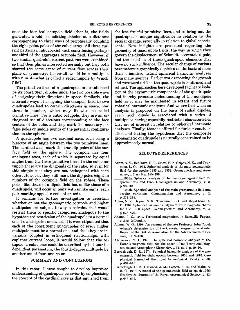
SELECTED REFERENCES 35
duce the identical octupole field (that is, the fields generated would be indistinguishable at a distance) corresponding to three ways of peripherally coupling the eight point poles of the cubic array. All three cur rent patterns might coexist, each contributing perhaps one-third of the aggregate octupole field. However, if two similar quatrefoil current patterns were combined so that their planes intersected normally but they both showed the same sense of current flow across their plane of symmetry, the result would be a multipole with n = 4—what is called a sedecimupole by Winch (1967).
The primitive lines of a quadrupole are established by its constituent dipoles under the two possible ways of assigning their directions in space. Similarly, the alternate ways of assigning the octupole field to two quadrupoles lead to certain directions in space, now three in number, which may likewise be called primitive lines. For a cubic octupole, they are an or thogonal set of directions corresponding to the face centers of the cube, and they mark the necessary six false poles or saddle points of the potential configura tion on the sphere.
A quadrupole has two cardinal axes, each being a bisector of an angle between the two primitive lines. The cardinal axes mark the true dip poles of the sur face field on the sphere. The octupole has four analogous axes, each of which is separated by equal angles from the three primitive lines. In the cubic oc tupole these are the diagonals of the cube, so even for this simple case they are not orthogonal with each other. However, they still mark the dip poles (eight in number) of the octupole field on the sphere. These poles, like those of a dipole field but unlike those of a quadrupole, will occur in pairs with unlike signs, each pair marking opposite ends of an axis.
It remains for further investigation to ascertain whether or not the geomagnetic octupole and higher multipoles are subject to any constraint that would restrict them to specific categories, analogous to the hypothesized restriction of the quadrupole to a normal one. To anticipate somewhat, if it were stipulated that each of the constituent quadrupoles of every higher multipole must be a normal one, and that they are in variably coupled in orthogonal relationships, with coplanar current loops, it would follow that the oc tupole (a cubic one) could be described by but four in dependent parameters, the fourth-degree multipole by another set of four, and so on.
SUMMARY AND CONCLUSIONS
In this report I have sought to develop improved understanding of quadrupole behavior by emphasizing the concept of the cardinal axes as distinguished from
the less fruitful primitive lines, and to bring out the quadrupole's unique significance in relation to the secular change, especially in relation to global constit uents. New insights are presented regarding the geometry of quadrupole fields, the way in which they govern the displacement of Schmidt's eccentric dipole, and the isolation of those quadrupole elements that have no such influence. The secular change of various parameters is graphically depicted on the basis of more than a hundred extant spherical harmonic analyses from many sources. Earlier work reporting the growth and westward drift of the quadrupole is confirmed and refined. The approaches here developed facilitate isola tion of the asymmetric components of the quadrupole and thereby promote understanding of the nondipole field as it may be manifested in extant and future spherical harmonic analyses. And we see that when an analysis is proposed on the basis of radial dipoles, every such dipole is associated with a series of multipoles having especially restricted characteristics that are of interest in relation to spherical harmonic analyses. Finally, there is offered for further consider ation and testing the hypothesis that the composite geomagnetic quadrupole is naturally constrained to be approximately normal.
SELECTED REFERENCES
Adam, N. V., Ben'kova, N. P., Orlov, V. P., Osipov.N. K., and Tyur- mina, L. O., 1962, Spherical analysis of the main geomagnetic field for the epochs 1955 and 1958: Geomagnetism and Aero- nomy, v. 2, no. 5, p. 785-796.
___1963a, Spherical analysis of the main geomagnetic field for epochs 1955 and 1958: Geomagnetism and Aeronomy, v. 3, p. 96-101.
_1963b, Spherical analysis of the main geomagnetic field andsecular variations: Geomagnetism and Aeronomy, v. 3, p. 271-285.
Adam, N. V., Osipov, N. K., Tyurmina, L. O., and Shlyakhtina, A. P., 1964, Spherical harmonic analysis of world magnetic charts for the 1960 epoch: Geomagnetism and Aeronomy, v. 4, p. 878-879.
Adams, J. C., 1900, Terrestrial magnetism, in Scientific Papers, v. 2, pt. 2: London.
Adams, W. G., 1898, An account of the late Professor John Couch Adams's determination of the Gaussian magnetic constants: Report of the British Association for the Advancement of Sci ence, p. 109-136.
Afanasieva, V. I., 1946, The spherical harmonic analysis of the Earth's magnetic field for the epoch 1945: Terrestrial Mag netism and Atmospheric Electricity, v. 51, no. 1, p. 19-30.
Barraclough, D. R., 1974, Spherical harmonic analyses of the geo magnetic field for eight epochs between 1600 and 1910: Geo physical Journal of the Royal Astronomical Society, v. 36, p. 497-513.
Barraclough, D. R., Harwood, J. M., Leaton, B. R., and Malin, S. R. C., 1975, A model of the geomagnetic field at epoch 1975: Geophysical Journal of the Royal Astronomical Society, v. 43, p. 645-659.
36 SELECTED REFERENCES
Bartels, J., 1936, The eccentric dipole approximating the Earth's magnetic field: Terrestrial Magnetism and Atmospheric Elec tricity, v. 41, p. 225-250.
Ben'kova, N. P., and Tyurmina, L. O., 1961, Analytical represen tation of the geomagnetic field over the territory of the Soviet Union for the 1958 epoch: Geomagnetism and Aeronomy, v. 1, no. 1, p. 81-96.
Bochev, A., 1965, The Earth's magnetic field represented as dipoles field: Bulgarska Akad. Naukite, Doklady (Comptes Rendus Academic Bulgare des Sciences), v. 18, p. 319-322.
Braginskii, S. I., 1969, Spherical analysis of the geomagnetic field from angular data and the extrapolated g? value: Geomag netism and Aeronomy, v. 9, p. 629-630.
___1972a, Spherical analyses of the geomagnetic field in 1550- 1800: Geomagnetism and Aeronomy, v. 12, p. 464-468.
_1972b, Analytical description of the geomagnetic field ofpast epochs and determination of the spectrum of magnetic waves in the core: Geomagnetism and Aeronomy, v. 12, p. 947-957.
Bullard, E. C., Freedman, C., Gellman, H., and Nixon, J., 1950, The westward drift of the Earth's magnetic field: Philosophical Transactions of the Royal Society of London, v. 243A, p. 67-92.
Cain, J. C., 1966, Models of the Earth's magnetic field, ire McCor- mac, B., ed., Radiation trapped in the Earth's magnetic field: Dordrecht, Netherlands, Reidel, p. 570-587.
Cain, J. C., and Cain, S. J., 1971, Derivation of the International Geomagnetic Reference Field (IGRF (10/68)): U.S. National Aeronautics and Space Administration, TN D-6237, 35 p.
Cain, J. C., Daniels, W. E., Hendricks, S. J., and Jensen, D. C., 1965, An evaluation of the main geomagnetic field, 1940-1962: Jour nal of Geophysical Research, v. 70, no. 15, p. 3647-3674.
Cain, J. C., Davis, W. M., and Regan, R. D., 1974, An re=22 model of the geomagnetic field [abs.]: Transactions of the American Geophysical Union, v. 55, no. 12, p. 1108.
Cain, J. C., Hendricks, S. J., Langel, R. A., and Hudson, W. V., 1967, A proposed model for the International Geomagnetic Ref erence Field—1965: Journal of Geomagnetism and Geoelectric- ity, v. 19, no. 4, p. 335-355.
Cain, J. C., and Sweeney, R. E., 1970, Magnetic field mapping of the inner magnetosphere: Journal of Geophysical Research, v. 75, no. 22, p. 4360-4362.
Carlheim-Gyllenskold, V., 1896, Sur la forme analytique de 1'at- traction magnetique de la Terre, exprimee en fonction du temps: Astronomiska iakttagelser och Undersb'k ningar pa Stockholms Observatorium, v. 5(5), 36 p. [Condensed English translation by L. A. Bauer in Terrestrial Magnetism and Atmospheric Elec tricity, v. 2, p. 150-155, 1897. Reviewed by A. Schmidt in Met. Zs., v. 14, p. 39-42, 1897. See also Arkiv foer matematik Astronomi och Fysik 3(7), 1906.]
Chakrabarty, S. K., 1954, The spherical harmonic analysis of the Earth's main magnetic field: Indian Journal of Meteorology and Geophysics, v. 5 (special no.), p. 63-66. [Coefficients also in Mauersberger (1952).]
Chapman, S., and Bartels, J., 1940, Geomagnetism, Volume 2: Oxford, Clarendon Press, 1049 p.
Chargoy, A., 1950, El caudripolo magnetico terrestre: Journal of Geophysical Research, v. 55, no. 1, p. 47-49.
Dickson, L. E., 1922, First course in the theory of equations: New York, Wiley. Pages unknown.
Dyson, F., and Furner, H., 1923, The Earth's magnetic potential: Monthly Notices, Royal Astronomical Society, Geophysical Supplement, v. 1, p. 76-88.
Erman, G. A., and Petersen, H., 1874, Die Grundlagen der Gaus- sishen Theorie und die Erscheinungen des Erdmagnetismus im Jahre 1829, mit Beriicksichtigung der Sa'kularvariationen aus alien vorliegenden Beobachtungen berechnet und dargestellt,
im Auftrag der Kaiserlichen Admiraltat: Berlin. Pages unknown. [Coefficients also given in Neumayer (1892) and in Adams (1898).]
Fabiano, E. B., and Peddie, N. W., 1975, U.S. world chart model coefficients for 1975: Transactions of the American Geophysical Union, v. 56, no. 9, p. 587-588.
Fanselau, G., and Kautzleben, H., 1958, Die analytische Darstel- lung des geomagnetischen Feldes: Geofisica Pura e Applicata, v. 41, p. 33-72.
Fanselau, G., Kautzleben, H., Lucke, O., Mauersberger, P., and Sellien, K., 1964, Die Darstellumg des geomagnetischen Po tentials zur Epoche 1945.0 durch eine Entwicklung nach Kugelfunktionen bis zur 15. Ordnung: Pure and Applied Geo physics, v. 57, p. 5-30.
Finch, H. F., and Leaton, B. R., 1957, The Earth's main magnetic field—epoch 1955.0: Monthly Notices Royal Astronomical So ciety, Geophysical Supplement, v. 7, p. 314-317. [The Gauss- normal coefficients (second solution) are used in the present study. Schmidt-normal ones are also given in the source paper, and likewise quoted by Nagata and Oguti (1962).]
Fougere, P. F., 1965, Spherical harmonic analysis—2, A new model derived from magnetic observatory data for epoch 1960.0: Jour nal of Geophysical Research, v. 70, no. 9, p. 2171-2179.
___1969, Spherical harmonic analysis—3, the Earth's magnetic field 1900-1965: Journal of Geomagnetism and Geoelectricity, v. 21, no. 3, p. 685-695.
Fritsche, H., 1897, Uber die Bestimmung der Koeffizienten der Gaussischen allgemeinen Theorie des Erdmagnetismus filr das Jahr 1885: St. Petersburg.
Gauss, C. F., 1839, Allgemeine Theorie des Erdmagnetismus, ire Resultate aus den Beobachtungen des magnetischen Vereins im Jahr 1838: Leipzig. Pages unknown. [Also his Werke, v. 5, p. 119-180, 1877. For English translation, see Richard Taylor, Scientific Memoirs 2, London, 1841. Coefficients also given in Neumayer (1892), in Quintus-Icilius (1881), and in Adams (1898).]
Harrison, C. G. A., 1975, Studying the Earth's field using the mag netization in sediments: Transactions of the American Geo physical Union, v. 56, no. 12, p. 977.
Hendricks, S. J., and Cain, J. C., 1966, Magnetic field data for trapped-particle evaluations: Journal of Geophysical Research, v.Tl.no. 1, p. 346-347.
Heppner, J. P., 1963, The World Magnetic Survey: Space Science Reviews, v. 2, p. 315-354.
Howe, H. H., 1939, The Earth's quadrupole moments: Transactions of the American Geophysical Union, v. 20, p. 359-364.
Humboldt, A., and Biot, J. B., 1804, Sur les variations du mag- netisme terrestre a diffeVentes latitudes: Journal de Physique, v. 59, p. 429-450. [Also English translation in Philosophical Magazine, v. 22, p. 248-257, p. 299-308,1805.]
Hurwitz, L., 1960, Eccentric dipoles and spherical harmonic analy sis: Journal of Geophysical Research, v. 65, no. 8, p. 2555-2556.
Hurwitz, L., and Fabiano, E. B., 1969, Geomagnetic secular vari ation 1937.5-1967.5 [abs.]: Bulletin of the International As sociation of Geomagnetism and Aeronomy, v. 26, p. 119. [The secular change has been applied retroactively to the AWC-70 model (see J 1965) to obtain the M group.]
Hurwitz, L., Fabiano, E. B., and Peddie, N. W., 1974, A model of the geomagnetic field for 1970: Journal of Geophysical Re search, v. 79, p. 1716-1717.
Hurwitz, L., Knapp, D. G., Nelson, J. H., and Watson, D. E., 1966, Mathematical model of the geomagnetic field for 1965: Journal of Geophysical Research, v. 71, no. 9, p. 2373-2381. [The mean coefficients in table 2 defined the model that became the CGS nominee, published also in Cain and Cain (1971). The "internal" model of table 1 is used in Group G (table 3 of this report).]
SELECTED REFERENCES 37
IAGA Commission 2 Working Group No. 4, 1969, Analysis of the geomagnetic field: Journal of Geophysical Research, v. 74, p. 4407.
Jensen, D. C., and Cain, J. C., 1962, An interim geomagnetic field [abs.]: Journal of Geophysical Research, v. 67, no. 9, p. 3568- 3569.
Jensen, D. C., and Whitaker, W. A., 1963, A spherical harmonic analysis of the geomagnetic field [abs.]: Journal of Geophysical Research, v. 65, no. 8, p. 2500. [Coefficients given in Heppner (1963).]
Jones, S. H., and Melotte, P. J., 1953, The harmonic analysis of the Earth's magnetic field for epoch 1942: Monthly Notices Royal Astronomical Society. Geophysical Supplement, v. 6, p.409-430.
Jory, F. S., 1956, Influence of geomagnetic quadrupole fields upon cosmic-ray intensity: The Physical Review, v. 102, p. 1167- 1173.
Kalinin, Yu. D., 1969, Determination of the parameters of an ar bitrarily oriented magnetic dipole, representing the geomag netic field: Geomagnetism and Aeronomy, v. 9, p. 854-855.
Kamtz, L. F., 1851, Correction of the constants in the general the ory of terrestrial magnetism: Proceedings Royal Philosophic Society, v. 6, p. 45-55.
Kautzleben, H., 1965a, Statistical analysis of the main part of the geomagnetic field, I: Geomagnetism and Aeronomy, v. 5, no. 3, p. 387-393.
_____1965b, Statistical analysis of the main part of the geomag netic field—II: Analysis of the world magnetic charts of the 1955.0 epoch: Geomagnetism and Aeronomy, v. 5, no. 3, p. 394-401.
Kelvin, W. T., Baron, 1872, A mathematical theory of magnetism, in Reprint of papers on electrostatics and magnetism: London, Macmillan, p. 344-592.
Leaton, B. R., Chmn., 1976, International Geomagnetic Reference Field 1975: Journal of Geophysical Research, v. 81, p. 5163- 5164.
Leaton, B. R., Malin, S. R. C., and Evans, M. J., 1965, An analyti cal representation of the estimated geomagnetic field and its secular change for the epoch 1965.0: Journal of Geomagnetism and Geoelectricity, v. 17, p. 187-194. [Coefficients also in Cain and Cain (1971).]
Lowes, F. J., Malin, S. R. C., and Saunders, I., 1974, Rotation of the geomagnetic field: Nature, v. 248, no. 5447, p. 402-405. [Criticism by Lowes of Malin and Saunders (1973) and their re joinder.]
Macht, H. G., 1950, The geomagnetic quadrupole moment: Journal of Geophysical Research, v. 55, p. 223-225.
Malin, S. R. C., 1969, Geomagnetic secular variation and its changes, 1942.5 to 1962.5: Geophysical Journal of the Royal Astronomi cal Society, v. 17, p. 415-441.
Malin, S. R. C., and Pocock, S. B., 1969, Geomagnetic spherical harmonic analysis: Pure and Applied Geophysics, v. 75, p. 117- 132.
Malin, S. R. C., and Saunders, I., 1973, Rotation of the Earth's magnetic field: Nature, v. 245, no. 5419, p. 25-26. [See also Lowes, Malin, and Saunders (1974).]
Mauersberger, P., 1952, A discussion of the variation with time of the parameters of the geomagnetic field based on the existing potential analyses: Abhandl. Geophys. Inst., Potsdam, no. 5, p. 9-58. [In German; English translation available: NASA TT-F- 8443 (1963).]
Maxwell, J. C., 1873: Treatise on electricity and magnetism, 2 vol umes: London. Pages unknown. [See esp. v. 1, p. 157, p. 160. Page references pertain to first edition.]
McDonald, K. L., and Gunst, R. H., 1967, An analysis of the Earth's magnetic field from 1835 to 1965: U.S. Dept. Commerce, ESSA
Tech. Rept., IER 46-IES 1, Boulder, Colo. Pages unknown.Nagata, T., 1965, Main characteristics of recent geomagnetic
secular variation: Journal of Geomagnetism and Geoelectricity, v. 17, p. 263-276.
Nagata, T., and Oguti, T., 1962, Magnetic charts for the epoch of 1958.5 corrected for the Antarctic region and spherical har monic coefficients of the revised geomagnetic field: Journal of Geomagnetism and Geoelectricity, v. 14, no. 2, p. 125-131.
Neumayer, G., 1892: Atlas des Erdmagnetismus (Berghaus's Phy- sikalischer Atlas, Abt. 4): Gotha, Justus Perthes. Pages un known.
Quintus-Icilius, G. Von, 1881, Der magnetische Zustand der Erde nach den von der Deutschen Seewarte herausgegebenen mag- netischen Karten fiir 1880.0: Hamburg, Archiv der Deutschen Seewarte, 4 (2). Pages unknown.
Schmidt, A., 1917, Erdmagnetismus, in Enzyklopaie der mathe- matischen Wissenschaften, mit Einschluss ihrer Anwendungen: Leipzig, B. G. Teubner, v. 6 (1), p. 266-396.
___1918, Geomagnetische Koordinaten, in Archiv des Erdmag netismus: Potsdam, Heft 3, p. 14.
___1934, Der magnetische Mittelpunkt der Erde und seine Be-deutung: Gerlands Beitrage zur Geophysik, v. 41, p. 346-358.
Tyurmina, L. O., 1968, Analytical model of the geomagnetic field according to Cosmos 49 data: Geomagnetism and Aeronomy, v. 8, p. 786-788.
Tyurmina, L. O., and Cherevko, T. N., 1967, Some results of a spher ical harmonic analysis of the geomagnetic field from Cosmos 49 data: Geomagnetism and Aeronomy, v. 7, p. 917. [For theory see v. 7, p. 207-210.]
Umov, N. A., 1904, Postroenie geometricheskogo obraza potentsi- ala Gaussa, kak priem izyskaniya zakonov zemnogo magnetiz- ma: Obschchestvo Liubitelei Estestvoznaniia Antropologii i Et- nografii, 107 (1). [Condensed German translation in Journal of Geophysical Research, v. 9, no. 3, p. 105-112.]
Vestine, E. H., 1953, On variations of the geomagnetic field, fluid motions, and the rate of the Earth's rotation: Journal of Geo physical Research, v. 58, no. 2, p. 127-145.
Vestine, E. H., Lange, I., LaPorte, L., and Scott, W. E., 1947, The geomagnetic field, its description and analysis: Carnegie In stitution of Washington, Publication 580.
Vestine, E. H., Sibley, W. L., Kern, J. W., and Carlstedt, J. L., 1963, Integral and spherical-harmonic analysis of the geomagnetic field for 1955.0, part 1: Journal of Geomagnetism and Geo electricity, v. 15, no. 2, p. 47-89.
Winch, D. E., 1967, The fourth-order geomagnetic multipole—the sedecimupole: Pure and Applied Geophysics, v. 67, p. 112-127.
Winch, D. E., and Malin, S. R. C., 1969, Changes in geomagnetic multipole parameters 1942.5-1962.5: Pure and Applied Geo physics, v. 74, p. 16-22.
Winch, D. E., and Slaucitajs, L., 1966, Geomagnetic multipoles, 1829 to 1960: Pure and Applied Geophysics, v. 63, p. 121-132. [Gives coefficients for several models including F 1932 and six averaged ones.]
Yukutake, T., 1971, Spherical harmonic analysis of the Earth's magnetic field for the 17th and 18th centuries: Journal of Geo magnetism and Geoelectricity, v. 23, no. 1, p. 11-31. [The Fritsche models are discussed also in Braginskii (1969).]
Zmuda, A. J., and Neuman, M., 1961, The correction and mutual dependence of harmonic coefficients, in Space Research: In ternational Space Science Symposium, 2nd, Florence, Pro ceedings, v. 2, p. 701-707. [Coefficients also given in McDonald and Gunst (1967).]
Zolotov, I. G., 1966, Representation of the geomagnetic field by means of multipoles: Geomagnetism and Aeronomy, v. 6, p. 413-421.
U.S. GOVERNMENT PRINTING OFFICE: 1979-677-129/22