Journal on Data Semantics manuscript No.(will be inserted by the editor)

On Modeling and Querying Concept Evolution

Siarhei Bykau · John Mylopoulos · Flavio Rizzolo · Yannis Velegrakis

Received: date / Accepted: date

Abstract Entities and the concepts they instantiate evolveover time. For example, a corporate entity may have resultedfrom a series of mergers and splits, or a concept such asthat of Whale may have evolved along with our understand-ing of the physical world. We propose a model for captur-ing and querying concept evolution. Our proposal extendsan RDF-like model with temporal features and evolutionoperators. In addition, we provide a query language thatexploits these extensions and supports historical queries.Moreover, we study how evolution information can be ex-ploited to answer queries that are agnostic to evolution de-tails (hence, evolution-unaware). For these, we propose dy-namic programming algorithms and evaluate their efficiencyand scalability by experimenting with both real and syn-thetic datasets.

Keywords Evolution · Possible worlds · Steiner Trees ·RDF · Query Answering

1 Introduction

Conceptual modeling languages – including the ER Model,UML class diagrams and Description Logics – are allfounded on a notion of entity that represents a thing in

Siarhei BykauUniversity of Trento Via Sommarive 14, Trento, ItalyE-mail: bykau@disi.unitn.eu

John MylopoulosUniversity of Trento Via Sommarive 14, Trento, ItalyE-mail: jm@disi.unitn.eu

Flavio RizzoloUniversity of Ottawa 800 King Edward St., Ottawa, CanadaE-mail: flavio@cs.toronto.edu

Yannis VelegrakisUniversity of Trento Via Sommarive 14, Trento, ItalyE-mail: velgias@disi.unitn.eu

the application domain. Although the state of an entity canchange over its lifetime, entities themselves are uniformlytreated as atomic and immutable. Unfortunately, this featureprevents existing modeling languages from capturing phe-nomena that involve the mutation of an entity into some-thing else, such as a caterpillar becoming a butterfly, or theevolution of one entity into several (or vice versa), such asGermany splitting off into two Germanies right after WWII.The same difficulty arises when we try to model evolutionat the class level. Consider the class Whale, which evolvedover the past two centuries in the sense that whales wereconsidered a species of fish, whereas today they are knownto be mammals. This means that the concept of Whale-as-mammal has evolved from that of Whale-as-fish in termsof the properties we ascribe to whales (e.g., their repro-ductive system). Clearly, the (evolutionary) relationship be-tween Whale-as-fish and Whale-as-mammal is of great in-terest to historians who may want to ask questions such as”Who studied whales in the past 3 centuries?” We are inter-ested in modeling and querying such evolutionary relation-ships between entities and/or classes. In the sequel, we referto both entities and classes as concepts.

In the database field, considerable amount of researcheffort has been spent on the development of models, tech-niques and tools for modeling and managing state changesfor a concept, but no work has addressed the forms of evo-lution suggested above. These range from data manipulationlanguages, and maintenance of views under changes (Blake-ley et al. 1986), to schema evolution (Lerner 2000) andmapping adaptation (Velegrakis et al. 2004; Kondylakis andPlexousakis 2010). To cope with the history of data changes,temporal models have been proposed for the relational (Soo1991) and ER (Gregersen and Jensen 1999) models, forsemi-structured data (Chawathe et al. 1999), XML (Rizzoloand Vaisman 2008) and for RDF (Gutierrez et al. 2005). Al-most in its entirety, existing work on data changes is based

2 Bykau et al.

on a state-oriented point of view. It aims at recording andmanaging changes that are taking place at the values of thedata.

In this work, we present a framework for modeling theevolution of concepts over time and the evolutionary rela-tionships among them. The framework allows posing newkinds of queries that previously could not have been ex-pressed. For instance, we aim at supporting queries of theform: How has a concept evolved over time? From what (or,to what) other concepts has it evolved? What other conceptshave affected its evolution over time? What concepts are re-lated to it through evolution and how? These kinds of queriesare of major importance for interesting areas which are suchas those discussed below.History. Modern historians are interested in studying thehistory of humankind, and the events and people whoshaped it. In addition, they want to understand how systems,tools, concepts of importance, and techniques have evolvedthroughout history. For them it is not enough to query a datasource for a specific moment in history. They need to askquestions on how concepts and the relationships that existbetween them have changed over time. For example, histo-rians may be interested in the evolution of countries such asGermany, with respect to territory, political division or lead-ership. Alternatively, they may want to study the evolutionof scientific concepts, e.g., how the concept of biotechnol-ogy has evolved from its humble beginnings as an agricul-tural technology to the current notion that is coupled to ge-netics and molecular biology.Entity Management. Web application and integration sys-tems are progressively moving from tuple and value-basedtowards entity-based solutions, i.e., systems where the ba-sic data unit is an entity, independently of its logical repre-sentation (Dong et al. 2005). Furthermore, web integrationsystems, in order to achieve interoperability, may need toprovide unique identification for the entities in the data theyexchange (Palpanas et al. 2008). However, entities do not re-main static over time: they get created, evolve, merge, split,and disappear. Knowing the history of each entity, i.e., howit has been formed and from what, paves the ground for suc-cessful entity management solutions and effective informa-tion exchange.Life Sciences. One of the fields in Biology focuses on thestudy of the evolution of species from their origins andthroughout history. To better understand the secrets of na-ture, it is important to model how the different species haveevolved, from what, if and how they have disappeared, andwhen. As established by Darwin’s theories, this evolution isvery important for the understanding of how species cameto be what they are now, or why some disappeared.

The contributions of this work are as follows: (i) We pro-pose a conceptual model enhanced with the notion of a life-time of a class, individual and relationship, (ii) We extend

the temporal model proposed in (Gutierrez et al. 2005) withconsistency conditions and additional constructs to modelmerges, splits, and other forms of evolution among con-cepts; (iii) We introduce an evolution-aware query languagethat supports the answering of queries regarding the life-time of concepts as well as the way they have evolved overtime; (iv) We offer a formal semantics of query answeringin the presence of evolution for queries that are evolutionunaware; (v) We implement the semantics of this query an-swering by generating on-the-fly possible instances (similarto the concept of possible worlds in probabilistic databases)where multiple concepts associated through evolution rela-tionships have been collapsed into one; (vi) We introducethe idea of finding a Steiner forest as a means of finding theoptimal merges that need to be done to generate the pos-sible instances and present indexing techniques for its ef-ficient implementation; (vii) We present the architecture ofthe system we have developed that incorporates the abovemethods; (viii) We describe a case study involving conceptevolution and perform a number of experiments for evaluat-ing our evolution-unaware query answering mechanism.

Preliminary versions of these contributions have beenpresented in two earlier publications (Rizzolo et al. 2009;Bykau et al. 2011). This paper extends and refines our ear-lier work by the following contributions: (a) We presentan integrative framework of the evolution management, i.e.both the modeling and query evaluation; (b) We describe thesystem architecture of the implementation of our researchideas; (c) We discuss the evolution discovery mechanismwhich is used to obtain a real data set for our experiments(the trademark dataset).

The rest of the paper is structured as follows. Section 2describes the motivating examples used in this work. In Sec-tion 3 we present our modeling framework for evolution-aware queries. A formal semantics of query answering inthe presence of evolution for queries that are evolution-unaware is discussed in Section 4. Section 5 presents the ar-chitecture of the system we have developed that incorporatesthe evolution-unaware evaluation methods. Two case stud-ies which involve evolution are described in Section 6. Thedescription of a number of experiments for evaluating ourevolution-unaware query answering mechanism is shown inSection 7. The related work is discussed in Section 8. Fi-nally, we conclude in Section 9.

2 Motivating ScenariosConsider a historian database that records information aboutcountries and their political governance. A fraction of thedatabase modeling a part of the history of Germany is illus-trated in Figure 1 (a). In it, the status of Germany at differenttimes in history has been modeled through different individ-uals or through different concepts. In particular, Germany

On Modeling and Querying Concept Evolution 3

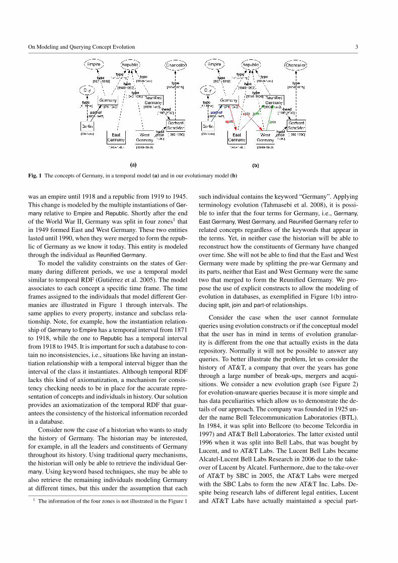
Fig. 1 The concepts of Germany, in a temporal model (a) and in our evolutionary model (b)

was an empire until 1918 and a republic from 1919 to 1945.This change is modeled by the multiple instantiations of Ger-many relative to Empire and Republic. Shortly after the endof the World War II, Germany was split in four zones1 thatin 1949 formed East and West Germany. These two entitieslasted until 1990, when they were merged to form the repub-lic of Germany as we know it today. This entity is modeledthrough the individual as Reunified Germany.

To model the validity constraints on the states of Ger-many during different periods, we use a temporal modelsimilar to temporal RDF (Gutierrez et al. 2005). The modelassociates to each concept a specific time frame. The timeframes assigned to the individuals that model different Ger-manies are illustrated in Figure 1 through intervals. Thesame applies to every property, instance and subclass rela-tionship. Note, for example, how the instantiation relation-ship of Germany to Empire has a temporal interval from 1871to 1918, while the one to Republic has a temporal intervalfrom 1918 to 1945. It is important for such a database to con-tain no inconsistencies, i.e., situations like having an instan-tiation relationship with a temporal interval bigger than theinterval of the class it instantiates. Although temporal RDFlacks this kind of axiomatization, a mechanism for consis-tency checking needs to be in place for the accurate repre-sentation of concepts and individuals in history. Our solutionprovides an axiomatization of the temporal RDF that guar-antees the consistency of the historical information recordedin a database.

Consider now the case of a historian who wants to studythe history of Germany. The historian may be interested,for example, in all the leaders and constituents of Germanythroughout its history. Using traditional query mechanisms,the historian will only be able to retrieve the individual Ger-many. Using keyword based techniques, she may be able toalso retrieve the remaining individuals modeling Germanyat different times, but this under the assumption that each

1 The information of the four zones is not illustrated in the Figure 1

such individual contains the keyword “Germany”. Applyingterminology evolution (Tahmasebi et al. 2008), it is possi-ble to infer that the four terms for Germany, i.e., Germany,East Germany, West Germany, and Reunified Germany refer torelated concepts regardless of the keywords that appear inthe terms. Yet, in neither case the historian will be able toreconstruct how the constituents of Germany have changedover time. She will not be able to find that the East and WestGermany were made by splitting the pre-war Germany andits parts, neither that East and West Germany were the sametwo that merged to form the Reunified Germany. We pro-pose the use of explicit constructs to allow the modeling ofevolution in databases, as exemplified in Figure 1(b) intro-ducing split, join and part-of relationships.

Consider the case when the user cannot formulatequeries using evolution constructs or if the conceptual modelthat the user has in mind in terms of evolution granular-ity is different from the one that actually exists in the datarepository. Normally it will not be possible to answer anyqueries. To better illustrate the problem, let us consider thehistory of AT&T, a company that over the years has gonethrough a large number of break-ups, mergers and acqui-sitions. We consider a new evolution graph (see Figure 2)for evolution-unaware queries because it is more simple andhas data peculiarities which allow us to demonstrate the de-tails of our approach. The company was founded in 1925 un-der the name Bell Telecommunication Laboratories (BTL).In 1984, it was split into Bellcore (to become Telcordia in1997) and AT&T Bell Laboratories. The latter existed until1996 when it was split into Bell Labs, that was bought byLucent, and to AT&T Labs. The Lucent Bell Labs becameAlcatel-Lucent Bell Labs Research in 2006 due to the take-over of Lucent by Alcatel. Furthermore, due to the take-overof AT&T by SBC in 2005, the AT&T Labs were mergedwith the SBC Labs to form the new AT&T Inc. Labs. De-spite being research labs of different legal entities, Lucentand AT&T Labs have actually maintained a special part-

4 Bykau et al.

Fig. 2 The history of the AT&T Labs.

nership relationship. All these different labs have produceda large number of inventions, as the respective patents candemonstrate. Examples of such inventions are VoIP (Voiceover Internet Protocol), the ASR (Automatic Speech Recog-nition), the P2P (Peer-to-Peer) Video and the laser. A graph-ical illustration of the above can be found in Figure 2 wherethe labs are modeled by rectangles and the patents by ovals.

Assume now a temporal database that models the aboveinformation. For simplicity we do not distinguish among thedifferent kinds of evolution relationships (split, merger, andso on). Consider a user who is interested in finding the labthat invented the laser and the ASR patent. It is true thatthese two patents have been filed by two different labs, theAT&T Bell Labs and the AT&T Labs Inc. Thus, the querywill return no results. However, it can be noticed that thelatter entity is an evolution of the former. It may be the casethat the user does not have the full knowledge of the waythe labs have changed or, in her own mind, the two labs arestill considered the same. We argue that instead of expectingfrom the user to know all the details of how the concept hasevolved and the way the data has been stored, which meansthat the user’s conceptual model should match the one of thedatabase, we’d like the system to try to match the user’s con-ceptual model instead. This means that the system shouldhave the evolution relationships represented explicitly andtake them into account when evaluating a query. In partic-ular, we want the system to treat the AT&T Bell Labs, theAT&T Labs Inc, and the AT&T Labs as one unified (virtual)entity. That unified entity is the inventor of both the laser andthe ASR, and should be the main element of the response tothe user’s query.

Of course, the query response is based on the assumptionthat the user did not intend to distinguish between the threeaforementioned labs. Since this is an assumption, it shouldbe associated with some degree of confidence. Such a degreecan be based, for instance, on the number of labs that had

to be merged in order to produce the answer. A responsethat involves 2 evolution-related entities should have higherconfidence than one involving 4.

As a similar example, consider a query asking for allthe partners of AT&T Labs Inc. Apart from those explicitlystated in the data (in the specific case, none), a traversal ofthe history of the labs can produce additional items in theanswer, consisting of the partners of its predecessors. Thefurther this traversal goes, the less likely it is that this is whatthe user wanted; thus, the confidence of the answer that in-cludes the partners of its predecessors should be reduced.Furthermore, if the evolution relationships have also an as-sociated degree of confidence, i.e., less than 100% certainty,the confidence computation of the answers should take thisinto consideration as well.

3 Supporting Evolution-Aware Queries

This section studies queries which are agnostic to evolu-tion details, namely the evolution-aware queries. In partic-ular, first we introduce the temporal database (Section 3.1),second we describe the evolution modeling technique (Sec-tion 3.2), finally we provide a formal definition of the querylanguage (Section 3.3) and briefly talk about its evaluationstrategy (Section 3.4).

3.1 Temporal Databases

We consider an RDF-like data model. The model is expres-sive enough to represent ER models and the majority of on-tologies and schemas that are used in practice (Lenzerini2002). It does not include certain OWL Lite features such assameAs or equivalentClass, since these features have beenconsidered to be outside of the main scope of this workand their omission does not restrict the functionality of themodel.

On Modeling and Querying Concept Evolution 5

We assume the existence of an infinite set of resourcesU , each with a unique resource identifier (URIs), and aset of literals L. A property is a relationship betweentwo resources. Properties are treated as resources them-selves. We consider the existence of the special proper-ties: rdfs:type, rdfs:domain, rdfs:range, rdfs:subClassOf andrdfs:subPropertyOf, which we refer to as type, dom, rng, subc,and subp, respectively. The set U contains three special re-sources: rdfs:Property, rdfs:Class and rdf:Thing, which we re-fer to as Prop, Class and Thing, respectively. The seman-tics of these resources as well as the semantics of the spe-cial properties are those defined in RDFS (W3C 2004). Re-sources are described by a set of triples that form a database.

Definition 1 A database Σ is a tuple 〈U,L, T 〉, whereU ⊆ U , L ⊆ L, T ⊆ U× U × U ∪ L, andU contains the resources rdfs:Property, rdfs:Class, andrdf:Thing. The set of classes of the database Σ is the setC=x | ∃〈x, type, rdfs:Class〉 ∈ T. Similarly, the set ofproperties is the set P=x | ∃〈x, type, rdfs:Property〉 ∈ T.The set P contains the RDFS properties type, dom, rng, subc,and subp. A resource i is said to be an instance of a classc ∈ C (or of type c) if ∃〈i, type, c〉 ∈ T . The set of instancesis the set I=i | ∃〈i, type, y〉 ∈ T.

A database can be represented as a hypergraph called anRDF graph. In the rest of the paper, we will use the termsdatabase and RDF graph equivalently.

Definition 2 An RDF graph of a database Σ is an hyper-graph in which nodes represent resources and literals andthe edges represent triples.

Example 1 Figure 1(a) is an illustration of an RDF Graph.The nodes Berlin and Germany represent resources. Theedge labeled part-of between them represents the triple〈Berlin,part-of,Germany〉. The label of the edge, i.e., part-of,represents a property.

To support the temporal dimension in our model, weadopt the approach of Temporal RDF (Gutierrez et al. 2005)which extends RDF by associating to each triple a timeframe. Unfortunately, this extension is not enough for ourgoals. We need to add time semantics not only to relation-ships between resources (what the triples represent), butalso to resources themselves by providing temporal-varyingclasses and individuals. This addition and the consistencyconditions we introduce below are our temporal extensionsto the temporal RDF data model.

We consider time as a discrete, total order domain Tin which we define different granularities. Following Dyre-son et al. (2000), a granularity is a mapping from integersto granules (i.e., subsets of the time domain T) such thatcontiguous integers are mapped to non-empty granules andgranules within one granularity are totally ordered and do

not overlap. Days and months are examples of two differentgranularities, in which each granule is a specific day in theformer and a month in the latter. Granularities define a latticein which granules in some granularities can be aggregatedin larger granules in coarser granularities. For instance, thegranularity of months is coarser than that of days becauseevery granule in the former (a month) is composed of aninteger number of granules in the latter (days). In contrast,months are not coarser (nor finer) than weeks.

Even though we model time as a point-based temporaldomain, we use intervals as abbreviations of sets of instantswhenever possible. An ordered pair [a, b] of time points,with a, b granules in a granularity, and a ≤ b, denotes theclosed interval from a to b. As in most temporal models,the current time point will be represented with the distin-guished word Now. We will use the symbol T to representthe infinite set of all the possible temporal intervals over thetemporal domain T, and the expressions i.start and i.endto refer to the starting and ending time points of an intervali. Given two intervals i1 and i2, we will denote by i1vi2the containment relationship between the intervals in whichi2.start≤i1.start and i1.end≤i2.end.

Two types of temporal dimensions are normally consid-ered: valid time and transaction time. Valid time is the timewhen data is valid in the modeled world whereas transactiontime is the time when data is actually stored in the database.Concept evolution is based on valid time.

Definition 3 A temporal database ΣT is a tuple〈U,L, T, τ〉, where 〈U,L, T 〉 is a database and τ isfunction that maps every resource r ∈ U to a temporalinterval in T . The temporal interval is also referred to asthe lifespan of the resource. The expressions r.start andr.end denote the start and end points of the interval of r,respectively. The temporal graph of ΣT is the RDF graphof 〈U,L, T 〉 enhanced with the temporal intervals on theedges and nodes.

For a temporal database to be semantically meaningful,the lifespans of the resources need to satisfy certain condi-tions. For instance, it is not logical to have an individual witha lifespan that does not contain any common time pointswith the lifespan of the class it belongs to. Temporal RDFdoes not provide such a mechanism, thus, we are introduc-ing the notion of a consistent temporal database.

Definition 4 A consistent temporal database is a temporaldatabase Στ=〈U,L, T, τ〉 that satisfies the following condi-tions:

1. ∀r ∈ L∪Prop,Class,Thing, type, dom, rng, subc, subp:τ(r)=[0, Now];

2. ∀〈d, p, r〉 ∈ T : τ(〈d, p, r〉)vτ(d) andτ(〈d, p, r〉)vτ(r);

3. ∀〈d, p, r〉 ∈ T with p ∈ type, subc, subp: τ(d)vτ(r).

6 Bykau et al.

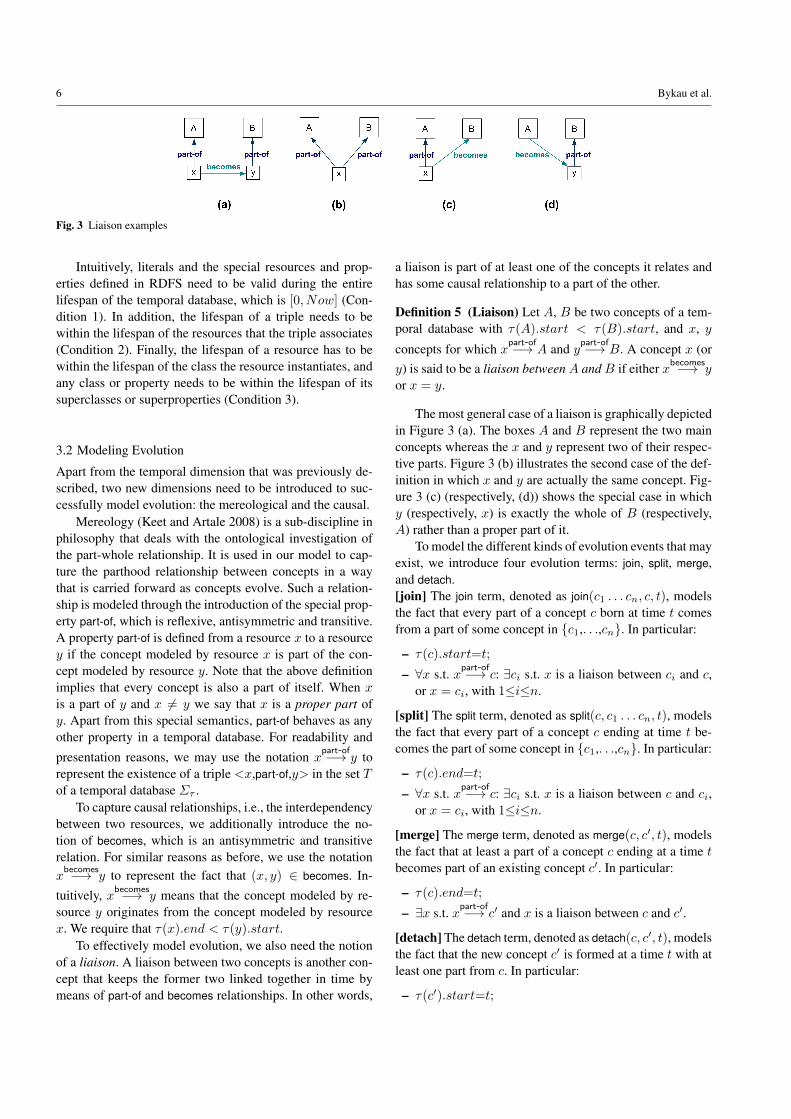
Fig. 3 Liaison examples

Intuitively, literals and the special resources and prop-erties defined in RDFS need to be valid during the entirelifespan of the temporal database, which is [0, Now] (Con-dition 1). In addition, the lifespan of a triple needs to bewithin the lifespan of the resources that the triple associates(Condition 2). Finally, the lifespan of a resource has to bewithin the lifespan of the class the resource instantiates, andany class or property needs to be within the lifespan of itssuperclasses or superproperties (Condition 3).

3.2 Modeling Evolution

Apart from the temporal dimension that was previously de-scribed, two new dimensions need to be introduced to suc-cessfully model evolution: the mereological and the causal.

Mereology (Keet and Artale 2008) is a sub-discipline inphilosophy that deals with the ontological investigation ofthe part-whole relationship. It is used in our model to cap-ture the parthood relationship between concepts in a waythat is carried forward as concepts evolve. Such a relation-ship is modeled through the introduction of the special prop-erty part-of, which is reflexive, antisymmetric and transitive.A property part-of is defined from a resource x to a resourcey if the concept modeled by resource x is part of the con-cept modeled by resource y. Note that the above definitionimplies that every concept is also a part of itself. When xis a part of y and x 6= y we say that x is a proper part ofy. Apart from this special semantics, part-of behaves as anyother property in a temporal database. For readability and

presentation reasons, we may use the notation xpart-of−→ y to

represent the existence of a triple <x,part-of,y> in the set Tof a temporal database Στ .

To capture causal relationships, i.e., the interdependencybetween two resources, we additionally introduce the no-tion of becomes, which is an antisymmetric and transitiverelation. For similar reasons as before, we use the notationxbecomes−→ y to represent the fact that (x, y) ∈ becomes. In-

tuitively, xbecomes−→ y means that the concept modeled by re-source y originates from the concept modeled by resourcex. We require that τ(x).end < τ(y).start.

To effectively model evolution, we also need the notionof a liaison. A liaison between two concepts is another con-cept that keeps the former two linked together in time bymeans of part-of and becomes relationships. In other words,

a liaison is part of at least one of the concepts it relates andhas some causal relationship to a part of the other.

Definition 5 (Liaison) Let A, B be two concepts of a tem-poral database with τ(A).start < τ(B).start, and x, y

concepts for which xpart-of−→ A and y

part-of−→ B. A concept x (ory) is said to be a liaison betweenA andB if either xbecomes−→ y

or x = y.

The most general case of a liaison is graphically depictedin Figure 3 (a). The boxes A and B represent the two mainconcepts whereas the x and y represent two of their respec-tive parts. Figure 3 (b) illustrates the second case of the def-inition in which x and y are actually the same concept. Fig-ure 3 (c) (respectively, (d)) shows the special case in whichy (respectively, x) is exactly the whole of B (respectively,A) rather than a proper part of it.

To model the different kinds of evolution events that mayexist, we introduce four evolution terms: join, split, merge,and detach.[join] The join term, denoted as join(c1 . . . cn, c, t), modelsthe fact that every part of a concept c born at time t comesfrom a part of some concept in c1,. . .,cn. In particular:

– τ(c).start=t;

– ∀x s.t. xpart-of−→ c: ∃ci s.t. x is a liaison between ci and c,

or x = ci, with 1≤i≤n.

[split] The split term, denoted as split(c, c1 . . . cn, t), modelsthe fact that every part of a concept c ending at time t be-comes the part of some concept in c1,. . .,cn. In particular:

– τ(c).end=t;

– ∀x s.t. xpart-of−→ c: ∃ci s.t. x is a liaison between c and ci,

or x = ci, with 1≤i≤n.

[merge] The merge term, denoted as merge(c, c′, t), modelsthe fact that at least a part of a concept c ending at a time tbecomes part of an existing concept c′. In particular:

– τ(c).end=t;

– ∃x s.t. xpart-of−→ c′ and x is a liaison between c and c′.

[detach] The detach term, denoted as detach(c, c′, t), modelsthe fact that the new concept c′ is formed at a time t with atleast one part from c. In particular:

– τ(c′).start=t;

On Modeling and Querying Concept Evolution 7

– ∃x s.t. xpart-of−→ c and x is a liaison between c and c′.

Note that in each evolution term there is only one con-cept whose lifespan has necessarily to start or end at the timeof the event. For instance, we could use a join to represent thefact that different countries joined the European Union (EU)at different times. The information of the period in whicheach country participated in the EU is given by the intervalof each respective part-of property.

We record the becomes relation and the evolution termsin the temporal database as evolution triples 〈c, term, c′〉,where term is one of the special evolution properties be-comes, join, split, merge, and detach. Evolution properties aremeta-temporal, i.e., they describe how the temporal modelchanges, and thus their triples do not need to satisfy theconsistency conditions in Definition 4. A temporal databasewith a set of evolution properties and triples defines an evo-lution base.

Definition 6 An evolution base ΣET is a tuple

〈U,L, T,E, τ〉, where 〈U,L, T, τ〉 is a temporal database,U contains a set of evolution properties, and E is a set ofevolution triples. The evolution graph ofΣE

T is the temporalgraph of 〈U,L, T, τ〉 enhanced with edges representing theevolutions triples.

The time in which the evolution event took place doesnot need to be recorded explicitly in the triple since it canbe retrieved from the lifespan of the involved concepts. Forinstance, detach(Kingdom of the Netherlands, Belgium, 1831)is modeled as the triple: 〈Kingdom of the Netherlands, detach,Belgium〉 with τ(Belgium).start = 1831.

For recording evolution terms that involve more than twoconcepts, e.g. the join, multiple triples are needed. We as-sume that the terms are indexed by their time, thus, the setof (independent) triples that belong to the same terms can beeasily detected since they will all share the same start or endtime in the lifespan of the respective concept. For instance,split(Germany, East Germany, West Germany, 1949) is repre-sented in our model through the triples 〈Germany, split, EastGermany〉 and 〈Germany, split, West Germany〉 with τ (EastGermany).start = τ(West Germany).start = 1949.

Note that the evolution terms may entail facts that are notexplicitly represented in the database. For instance, the splitof Germany into West and East implies the fact that Berlin,which is explicitly defined as part of Germany, becomes partof either East or West. This kind of reasoning is beyond thescope of the current work.

3.3 Query Language

To support evolution-aware querying we define a naviga-tional query language to traverse temporal and evolutionedges in an evolution graph. This language is analogous

to nSPARQL (Perez et al. 2008), a language that extendsSPARQL with navigational capabilities based on nested reg-ular expressions. nSPARQL uses four different axes, namelyself , next, edge, and node, for navigation on an RDFgraph and node label testing. We have extended the nestedregular expressions constructs of nSPARQL with temporalsemantics and a set of five evolution axes, namely join,

split, merge, detach, and becomes that extend thetraversing capabilities of nSPARQL to the evolution edges.The language is defined according to the following gram-mar:

exp := axis | t-axis :: a | t-axis :: [exp] |exp[I] | exp/exp | exp|exp | exp∗

where a is a node in the graph, I is a time in-terval, and axis can be either forward, backward,e-edge, e-node, a t-axis or an e-axis, with t-axis ∈self , next, edge, node and e-axis ∈ join, split,merge, detach, becomes.

The evaluation of an evolution expression exp is givenby the semantic function E defined in Figure 4. E [[exp]] re-turns a set of tuples of the form 〈x, y, I〉 such that thereis a path from x to y satisfying exp during interval I .For instance, in the evolution base of Figure 1, E [[self ::

Germany/next :: head/next :: type]] returns the tuple〈Germany, Chancellor, [1988, 2005]〉. It is also possible tonavigate an edge from a node using the edge axis and tohave a nested expression [exp] that functions as a predi-cate which the preceding expression must satisfy. For ex-ample, E [[self [next :: head/self :: Gerhard Schroder]]] re-turns 〈Reunified Germany, Reunified Germany, [1990, 2005]〉and 〈West Germany, West Germany, [1988, 1990]〉.

In order to support evolution expressions, we need toextend nSPARQL triple patterns with temporal and evolu-tion semantics. In particular, we redefine the evaluation ofan nSPARQL triple pattern (?X, exp, ?Y ) to be the set oftriples 〈x, y, I〉 that result from the evaluation of the evolu-tion expression exp, with the variables X and Y bound to xand y, respectively. In particular:

E [[(?X, exp, ?Y )]] := (θ(?X), θ(?Y )) | θ(?X) = x and

θ(?Y ) = y and 〈x, y, I〉 ∈ E [[exp]]

Our language includes all nSPARQL operators such asAND, OPT, UNION and FILTER with the same semanticsas in nSPARQL. For instance:

E [[(P1 AND P2)]] := E [[(P1)]] ./ E [[(P2)]]

where P1 and P2 are triple patterns and ./ is the join onthe variables P1 and P2 have in common. A complete listof all the nSPARQL operators and their semantics is givenby (Perez et al. 2008).

8 Bykau et al.

E[[self ]] := 〈x, x, τ(x)〉 |x ∈ U∪LE[[self ::r]] := 〈r, r, τ(r)〉E[[next]] := 〈x, y, τ(t)〉 | t = 〈x, z, y〉 ∈ T

E[[next ::r]] := 〈x, y, τ(t)〉 | t = 〈x, r, y〉 ∈ TE[[edge]] := 〈x, y, τ(t)〉 | t = 〈x, y, z〉 ∈ T

E[[edge ::r]] := 〈x, y, τ(t)〉 | t = 〈x, y, r〉 ∈ TE[[node]] := 〈x, y, τ(t)〉 | t = 〈z, x, y〉 ∈ T

E[[node ::r]] := 〈x, y, τ(t)〉 | t = 〈r, x, y〉 ∈ TE[[e-edge]] := 〈x, e-axis, [0, Now]〉 | t = 〈x, e-axis, z〉 ∈ EE[[e-node]] := 〈e-axis, y, τ(t)〉 | t = 〈z, e-axis, y〉 ∈ EE[[e-axis]] := 〈x, y, [0, Now]〉 | ∃ t = 〈x, e-axis, y〉 ∈ E

E[[forward]] :=⋃

e-axis E[[e-axis]]E[[backward]] :=

⋃e-axis E[[e-axis−1]]

E[[self :: [exp]]] := 〈x, x, τ(x)∩ I〉 |x ∈ U∪L, ∃〈x, z, I〉 ∈ P[[exp]], τ(x)∩I 6= ∅E[[next :: [exp]]] := 〈x, y, τ(t)∩I〉 | t = 〈x, z, y〉 ∈ T , ∃〈z, w, I〉 ∈ P[[exp]], τ(t)∩I 6= ∅E[[edge :: [exp]]] := 〈x, y, τ(t)∩I〉 | t = 〈x, y, z〉 ∈ T , ∃〈z, w, I〉 ∈ P[[exp]], τ(t)∩I 6= ∅E[[node :: [exp]]] := 〈x, y, τ(t)∩I〉 | t = 〈z, x, y〉 ∈ T , ∃〈z, w, I〉 ∈ P[[exp]], τ(t)∩I 6= ∅

E[[axis−1]] := 〈x, y, τ(t)〉 | 〈y, x, τ(t)〉 ∈ E[[axis]]E[[t-axis−1 ::r]] := 〈x, y, τ(t)〉 | 〈y, x, τ(t)〉 ∈ E[[t-axis ::r]]

E[[t-axis−1 :: [exp]]] := 〈x, y, τ(t)〉 | 〈y, x, τ(t)〉 ∈ E[[t-axis :: [exp]]]E[[exp[I]]] := 〈x, y, I∩I′〉 | 〈x, y, I′〉 ∈ E[[exp]] and I∩I′ 6= ∅

E[[exp/e-exp]] := 〈x, y, I2〉 | ∃〈x, z, I1〉 ∈ E[[exp]], ∃〈z, y, I2〉 ∈ E[[e-exp]]E[[exp/t-exp]] := 〈x, y, I1∩I2〉 | ∃〈x, z, I1〉 ∈ E[[exp]], ∃〈z, y, I2〉 ∈ E[[t-exp]] and

I1∩I2 6= ∅E[[exp1|exp2]] := E[[exp1]] cupE[[exp2]]

E[[exp∗]] := E[[self ]] ∪ E[[exp]] ∪ E[[exp/exp]] ∪ E[[exp/exp/exp]] ∪ . . .

P[[e-exp]] := E[[e-exp]]P[[t-exp]] := E[[t-exp]]

P[[t-exp/exp]] := 〈x, y, I1∩I2〉 | ∃〈x, z, I1〉 ∈ E[[t-exp]], ∃〈z, y, I2〉 ∈ E[[exp]] andI1∩I2 6= ∅

P[[e-exp/exp]] := 〈x, y, I1〉 | ∃〈x, z, I1〉 ∈ E[[e-exp]], ∃〈z, y, I2〉 ∈ E[[exp]]P[[exp1|exp2]] := E[[exp1|exp2]]

P[[exp∗]] := E[[exp∗]]

t-exp ∈ t-axis, t-axis ::r, t-axis :: [exp], t-axis[I]e-exp ∈ e-axis, e-axis :: [exp], e-axis[I], forward,backward

Fig. 4 Formal semantics of nested evolution expressions

3.4 Query Evaluation

The query language presented in the previous section isbased on the concepts of nSPARQL and can be implementedas an extension of it by creating the appropriate query rewrit-ing procedures that implement the semantics of Figure 4.Since our focus in query evaluation strategies is mainly onthe evolution-unaware queries, we will not elaborate furtheron this.

4 Supporting Evolution-Unaware Queries

In this section we discuss the evolution-unaware queries. Inparticular, we present the model of evolution in Section 4.1,then we show a number of query evaluation techniques start-ing from naive ways and ending up with our solution (Sec-tion 4.2). In Section 4.3 we introduce the Steiner forest algo-rithm, which constitutes the core of our evaluation strategy,along with an optimization technique.

4.1 Modeling Evolution

To support queries that are unaware of the evolution rela-tionships we need to construct a mechanism that performsvarious kinds of reasoning in a way transparent to the user.This reasoning involves the consideration of a series of datastructures associated through the evolution relationships asone unified concept. For simplicity of the presentation, andalso to abstract from the peculiarities of RDF, in what fol-lows we use a concept model (Dalvi et al. 2009) as our datamodel. Furthermore, we do not consider separately the dif-ferent kinds of evolution events but we consider them allunder one unified relationship that we call evolve. This al-lows us to focus on different aspects of our proposal withoutincreasing its complexity.

The fundamental component of the model is the concept,which is used to model a real world object. A concept is adata structure consisting of a unique identifier and a set ofattributes. Each attribute has a name and a value. The valueof an attribute can be an atomic value or a concept identi-

On Modeling and Querying Concept Evolution 9

fier. More formally, assume the existence of an infinite setof concept identifiers O, an infinite set of names N and aninfinite set of atomic values V .Definition 7 An attribute is a pair 〈n,v〉, with n∈N andv∈V∪O. Attributes for which v∈O are specifically referredto as associations. Let A=N×V∪O be the set of all thepossible attributes. A concept is a tuple 〈id,A〉whereA⊆A,is finite, and id∈O. The id is referred to as the concept iden-tifier while the set A as the set of attributes of the concept.

We will use the symbol E to denote the set of all possibleconcepts that exist and we will also assume the existence ofa Skolem function Sk (Hull and Yoshikawa 1990). Recallthat a Skolem function is a function that guarantees that dif-ferent arguments are assigned different values. Each conceptis uniquely identified by its identifier, thus, we will often usethe terms concept and concept identifier interchangingly ifthere is no risk of confusion. A database is a collection ofconcepts, that is closed in terms of associations between theconcepts.Definition 8 A database is a finite set of concepts E⊆Esuch that for each association 〈n, e′〉 of a concept e∈E:e′∈E.

As a query language we adopt a datalog style language.A query consists of a head and a body. The body is a con-junction of atoms. An atom is an expression of the forme(n1:v1, n2:v2, . . ., nk:vk) or an arithmetic condition suchas =, ≤, etc. The head is always a non-arithmetic atom.Given a database, the body of the query is said to be true ifall its atoms are true. A non-arithmetic atom e(n1:v1, n2:v2,. . ., nk:vk) is true if there is a concept with an identifier eand attributes 〈ni, vi〉 for every i=1..k. When the body ofa query is true, the head is also said to be true. If a heade(n1:v1, n2:v2, . . ., nk:vk) is true, the answer to the queryis a concept with identifier e and attributes 〈n1:v1〉, 〈n2:v2〉,. . ., 〈nk:vk〉.

The components e, ni and vi, for i=1..k of any atomin a query can be either a constant or a variable. Variablesused in the head or in arithmetic atoms must also be used insome non-arithmetic atom in the body. If a variable is usedat the beginning of an atom, it is bound to concept identi-fiers. If the variable is used inside the parenthesis but beforethe “:“ symbol, it is bound to attribute names, and if the vari-able is in the parenthesis after the “:“ symbol, it is bound toattribute values. A variable assignment in a query is an as-signment of its variables to constants. A true assignment isan assignment that makes the body of the query true. Theanswer set of a query involving variables is the union of theanswers produced by the query for each true assignment.

Example 2 Consider the query:$x(isHolder:$y):-

$x(name:′AT&TLabsInc.′, isHolder:$y)

that looks for concepts called “AT&T Labs Inc.” and are

holders of a patent. For every such concept that is found,a concept with the same identifier is produced in the answerset and has an attribute isHolder with the patent as a value.

In order to model evolution we need to model the lifes-pan of the real world objects that the concepts represent andthe evolution relationship between them. For the former, weassume that we have a temporal database, i.e., each con-cept is associated to a time period (see Section 3.1); how-ever, this is not critical for the evolution-unaware queriesso we will omit that part from the following discussions.To model the evolution relationship for evolution-unawarequeries we consider a special association that we elevate intoa first-class citizen in the database. We call this associationan evolution relationship. Intuitively, an evolution relation-ship from one concept to another is an association indicatingthat the real world object modeled by the latter is the resultof some form of evolution of the object modeled by the for-mer. Note that the whole family of evolution operators fromSection 3.2 is reduced to only one relationship.

In the next, with the abuse of notation we re-introducethe notion of evolution database with respect to theevolution-unaware queries. This allows us to focus onlyon the parts of our data model which are essential tothe evolution-unaware queries. In Figure 2, the dottedlines between the concepts illustrate evolution relationships.A database with evolution relationships is an evolutiondatabase.

Definition 9 An evolution database is a tuple 〈E,Ω〉, suchthat 〈E〉 is a database and Ω is a partial order rela-tion over E. An evolution relationship is every association(e1, e2)∈Ω.

Given an evolution database, one can construct a di-rected acyclic graph by considering as nodes the conceptsand as edges its evolution relationships. We refer to thisgraph as the evolution graph of the database.

Our proposal is that concepts representing different evo-lution phases of the same real world object can be con-sidered as one for query answering purposes. To formallydescribe this idea we introduce the notion of coalescence.Coalescence is defined only on concepts that are connectedthrough a series of evolution relationships; the coalescenceof those concepts is a new concept that replaces them andhas as attributes the union of their attributes (including asso-ciations).

Definition 10 Given an evolution database 〈E,Ω〉, The coa-lescence of two concepts e1:〈id1,A1〉, e2:〈id2,A2〉∈E, con-nected through an evolution relationship ev is a new evo-lution database 〈E′,Ω′〉 such that Ω′=Ω−ev and E′=(E− e1, e2) ∪ enew, where enew:〈idnew,Anew〉 is a newconcept with a fresh identifier idnew=Sk(id1, id2) andAnew=A1∪A2. Furthermore, each association 〈n,id1〉 or

10 Bykau et al.

〈n,id2〉 of an concept e∈E, is replaced by 〈n,idnew〉. Therelationship between the two databases is denoted as 〈E,Ω〉ev−→ 〈E′,Ω′〉

The Skolem function that we have mentioned earlier de-fines a partial order among the identifiers, and this partialorder extends naturally to concepts. We call that order sub-sumption.

Definition 11 An identifier id1 is said to be subsumed byan identifier id, denoted as id1

.≺id if there is some identi-

fier idx 6=id and idx 6=id1 such that id=Sk(id1, idx). A con-cept e1=〈id1, A1〉 is said to be subsummed by a concepte2=〈id2, A2〉, denoted as e1

.≺e2, if id1

.≺id2 and for ev-

ery attribute 〈n,v1〉∈A1 there is attribute 〈n,v2〉∈A2 suchthat v1=v2 or, assuming that the attribute is an association,v1.≺v2.

Given an evolution database 〈E,Ω〉, and a setΩs⊆Ω onecan perform a series of consecutive coalescence operations,each one coalescing the two concepts that an evolution rela-tionship in the Ωs associates.

Definition 12 Given an evolution database D:〈E,Ω〉 and aset Ωs=m1, m2, . . . , mm such that Ωs⊆Ω, let Dm bethe evolution database generated by the sequence of coales-cence operations D

m1−→D1m2−→, . . . ,

mm−→Dm. The possibleworld of D according to Ωs is the database DΩs

generatedby simply omitting from Dm all its evolution relationships.

Intuitively, a set of evolution relationships specifies setsof concepts in a database that should be considered as one,while the possible world represents the database in whichthese concepts have actually been coalesced. Our notion of apossible world is similar to the notion of a possible worlds inprobabilistic databases (Dalvi and Suciu 2007). Theorem 1is a direct consequence of the definition of a possible world.

Theorem 1 The possible world of an evolution databaseD:〈E,Ω〉 for a set Ωs⊆Ω is unique.

Due to this uniqueness, a set Ωs of evolution relation-ships of a database can be used to refer to the possible world.

According to the definition of a possible world, an evo-lution database can be seen as a shorthand of a set ofdatabases, i.e., its possible worlds. Thus, a query on an evo-lution database can be seen as a shorthand for a query onits possible worlds. Based on this observation we define thesemantics of query answering on an evolution database.

Definition 13 The evaluation of a query q on an evolutiondatabase D is the union of the results of the evaluation ofthe query on every possible world Dc of D.

For a given query, there may be multiple possible worldsthat generate the same results. To eliminate this redundancywe require every coalescence to be well-justified. In partic-ular, our principle is that no possible world or variable as-signment will be considered, unless it generates some newresults in the answer set. Furthermore, among the different

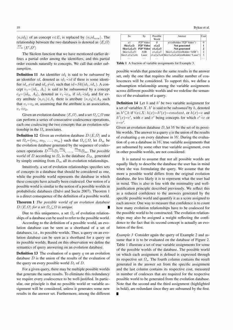
$x $y Possible Answer CostWorld

e1 P2P Video ∅ e1(isHolder:“P2P Video”) 0Sk(e1,e2) P2P Video e1,e2 Not generated 1

Sk(e1,e2,e3) P2P Video e1,e2,e3 Not generated 2Sk(e1,e2,e3) ASR e1,e2,e3 Sk(e1,e2,e3)(isHolder:“ASR”) 2

Sk(e1,e2,e3,e4) Laser e1,e2,e3,e4 Sk(e1,e2,e3,e4)(isHolder:“Laser”) 3. . . . . . . . . . . . . . .

Table 1 A fraction of variable assignments for Example 3.

possible worlds that generate the same results in the answerset, only the one that requires the smaller number of coa-lescences will be considered. To support this, we define asubsumption relationship among the variable assignmentsacross different possible worlds and we redefine the seman-tics of the evaluation of a query.

Definition 14 Let h and h′ be two variable assignment fora set of variables X . h′ is said to be subsumed by h, denotedas h′⊆h if ∀x∈X: h(x)=h′(x)=constant, or h(x)=e andh′(x)=e′, with e and e′ being concepts for which e′

.≺e or

e=e′.Given an evolution database D, letW be the set of its possi-ble worlds. The answer to a query q is the union of the resultsof evaluating q on every database inW . During the evalua-tion of q on a database inW , true variable assignments thatare subsumed by some other true variable assignment, evenin other possible worlds, are not considered.

It is natural to assume that not all possible worlds areequally likely to describe the database the user has in mindwhen she was formulating the query. We assume that themore a possible world differs from the original evolutiondatabase, the less likely it is to represent what the user hadin mind. This is also in line with the minimality and well-justification principle described previously. We reflect thisas a reduced confidence to the answers generated by thespecific possible world and quantify it as a score assigned toeach answer. One way to measure that confidence is to counthow many evolution relationships have to be coalesced forthe possible world to be constructed. The evolution relation-ships may also be assigned a weight reflecting the confi-dence to the fact that its second concept is actually an evo-lution of the first.

Example 3 Consider again the query of Example 2 and as-sume that it is to be evaluated on the database of Figure 2.Table 1 illustrate a set of true variable assignments for someof the possible worlds of the database. The possible worldon which each assignment is defined is expressed throughits respective set Ωs. The fourth column contains the resultgenerated in the answer set from the specific assignmentand the last column contains its respective cost, measuredin number of coalesces that are required for the respectivepossible world to be generated from the evolution database.Note that the second and the third assignment (highlightedin bold), are redundant since they are subsumed by the first.

On Modeling and Querying Concept Evolution 11

The existence of a score for the different solutions, al-lows us to rank the query results and even implement a top-k query answering. The challenging task though is how toidentify in an efficient way the possible worlds and morespecifically the true variable assignments that lead into cor-rect results.

4.2 Query Evaluation

In this section we present evaluation strategies for theevolution-unaware queries, namely the naive approach (Sec-tion 4.2.1), the materializing all the possible worlds method(Section 4.2.2), the materializing only the maximum worldapproach(Section 4.2.3) and, finally, the on-the-fly coales-cence computations (Section 4.2.4).

4.2.1 The naive approach

The straightforward approach in evaluating a query is togenerate all the possible worlds and evaluate the query oneach one individually. In the sequel, generate the union ofall the individually produced results, eliminate duplicationand remove answers subsumed by others. Finally, associateto each of the remaining answers a cost based on the coa-lescences that were performed in order to generate the pos-sible world from which the answer was produced, and rankthe answers according to that score. The generation of allpossible worlds is a time consuming task. For an evolutiondatabase with an evolution graph of N edges, there are 2N

possible worlds. This is clearly a brute force solution, notdesirable for online query answering.

4.2.2 Materializing all the possible worlds

Since the possible worlds do not depend on the query thatneeds to be evaluated, they can be pre-computed and storedin advance so that they are available at query time. Ofcourse, as it is the case of any materialization technique,the materialized data need to be kept in sync with the evo-lution database when its data is modified. Despite the factthat this will require some effort, there are already well-known techniques for change propagation (Blakeley et al.1986) that can be used. The major drawback, however, is thespace overhead. A possible world contains all the attributesof the evolution database, but in fewer concepts. Given thatthe number of attributes are typically larger than the numberof concepts, and that concepts associated with evolution re-lationships are far fewer than the total number of concepts inthe database, we can safely assume that the size of a possi-ble world will be similar to the one of the evolution database.Thus, the total space required will be 2n times the size of theevolution database. The query answering time, on the other

hand, will be 2n times the average evaluation time of thequery on a possible world.

4.2.3 Materializing only the maximum world

An alternative solution is to generate and materialize thepossible world Dmax generated by performing all possiblecoalescences. For a given evolution database 〈E,Ω〉, thisworld is the one constructed according to the set of all evo-lution relationships in Ω. Any query that has an answer insome possible world of the evolution database will also havean answer in this maximal possible world Dmax. This solu-tion work has two main limitations. First it does not followour minimalistic principle and performs coalescences thatare not needed, i.e., they do not lead to any additional resultsin the result set. Second, the generated world fails to includeresults that distinguish difference phases of the lifespan ofa concept (phases that may have to be considered individ-ual concepts) but the approach coalesces them in one justbecause they are connected through evolution relationships.

4.2.4 On-the-fly coalescence computations

To avoid any form of materialization, we propose an alter-native technique that computes the answers on the fly byperforming coalescences on a need-to-do basis. In particu-lar, we identify the attributes that satisfy the different queryconditions and from them the respective concepts to whichthey belong. If all the attributes satisfying the conditions areon the same concept, then the concept is added in the an-swer set. However, different query conditions may be sat-isfied by attributes in different concepts. In these cases weidentify sets of concepts for each one of which the union ofthe attributes of its concepts satisfy all the query conditions.For each such a set, we coalesce all its concepts into one ifthey belong to the same connected component of the evolu-tion graph. Doing the coalescence it is basically like creatingthe respective possible world; however, we generate only thepart of that world that is necessary to produce an answer tothe query. In more details, the steps of the algorithm are thefollowing.

[Step 1: Query Normalization] We decompose ev-ery non-arithmetic atom in the body of the query thathas more than one condition into a series of single-condition atoms. More specifically, any atom of the formx(n1:v1, n2:v2, . . . , nk:vk) is decomposed into a conjunc-tion of atoms x(n1:v1), x(n2:v2), . . . , x(nk:vk).

[Step 2: Individual Variable Assignments Generation]For each non-arithmetic atom in the decomposed query, alist is constructed that contains assignments of the variablesin the respective atom to constants that make the atom true.Assuming a total of N non-arithmetic atoms after the de-composition, let L1, L2, . . . , LN be the generated lists. Each

12 Bykau et al.

variable assignment actually specifies the part of the evo-lution database that satisfies the condition described in theatom.

[Step 3: Candidate Assignment Generation] The ele-ments of the lists generated in the previous step are com-bined together to form complete variable assignments, i.e.,assignments that involve every variable in the body of thequery. In particular, the cartesian product of the lists is cre-ated. Each element in the cartesian product is a tuple of as-signments. By construction, each such tuple will contain atleast one assignment for every variable that appears in thebody of the query. If there are two assignments of the sameattribute bound variable to different values, the whole tupleis rejected. Any repetitive assignments that appear withineach non-rejected tuple is removed to reduce redundancy.The result is a set of variable assignments, one from each ofthe tuples that have remained.

[Step 4: Arithmetic Atom Satisfaction Verification] Eachassignment generated in the previous step for which there isat least one arithmetic atom not evaluating to true, is elimi-nated from the list.

[Step 5: Candidate Coalescence Identification] Withineach of the remaining assignments we identify concept-bound variables that have been assigned to more than onevalues. Normally this kind of assignment evaluates alwaysto false. However, we treat them as suggestions for coales-cences, so that the assignment will become a true assign-ment (ref. previous Section). For each assignment h in thelist provided by Step 4, the set Vh=Vx1 , Vx2 , . . . , Vxk

is generated, where Vx is the set of different concepts thatvariable x has been assigned in assignment h. In order forthe assignments of variable x to evaluate to true, we needto be able to coalesce the concepts in Vx. To do so, theseconcepts have to belong to the same connected componentin the evolution graph of the database. If this is not the case,the assignment h is ignored.

[Step 6: Coalescence Realization & Cost Computation]Given a set Vh=Vx1

, Vx2, . . . , Vxk

for an assignment hamong those provided by Step 5, we need to find the mini-mum cost coalescences that need to be done such that all theconcepts in a set Vi, for i=1..k, are coalesced to the sameconcept. This will make the assignment h a true assignment,in which case the head of the query can be computed and ananswer generated in the answer set. The cost of the answerwill be the cost of the respective possible world, which ismeasured in terms of the number of coalescences that needto be performed. Finding the required coalescences for theset Vh that minimizes the cost boils down to the problem offinding a Steiner forest (Gassner 2010),

Example 4 Let us consider again the query of Example 2.In Step 1, its body will be decomposed into two parts:

$x(name:′AT&TLabsInc.′) and $x(isHolder:$y). Forthose two parts, during Step 2, the lists L1=$x=e1 andL2=$x=e1, $y=′P2PV ideo′, $x=e3, $y=′ASR′,$x=e4, $y=′Laser′, $x=e5, $y=′V oIP ′ will becreated. Step 3 creates their cartesian product L=$x=e1,$x=e1, $y=′P2PV ideo′, $x=e1, $x=e3, $y=′ASR′,$x=e1, $x=e4, $y=′Laser′, $x=e1, $x=e5,$y=′V oIP ′. The only attribute bound variable is$y but this is never assigned to more than one differentvalue at the same time so nothing is eliminated. Sincethere are no arithmetic atoms, Step 4 makes no changeeither to the list L. If for instance, the query had an atom$y 6=′V OIP ′ in its body, then the last element of the listwould have been eliminated. Step 5 identifies that the lastthree elements in L have the concept bound variable $x

assigned to two different values; thus, it generates thecandidate coalesences: V1=e1, e3, V2=e1, e4 andV3=e1, e5. Step 6 determines that all three coalescencesare possible. Concepts e1, e2 and e3 will be coalesced forV1, e1, e2, e3 and e4 for V2, and the e1, e2, e3 and e5 forV3.

4.3 Steiner Forest Algorithm

The last step of the evaluation algorithm for evolution un-aware query language takes as input a set of concept setsand needs to perform a series of coalesce operations suchthat all the concepts within each set will become one. To doso, it needs to find an interconnect on the evolution graphamong all the concepts within each set. Note that the inter-connect may involve additional concepts not in the set thatunavoidably will also have to be coalesced with those in theset. Thus, it is important to find an interconnect that mini-mizes the total cost of the coalescences. The cost of a coa-lescence operation is the weight of the evolution relationshipthat connects the two concepts that are coalesced. Typically,that cost is equal to one, meaning that the total cost is actu-ally the total number of coalescence operations that need tobe performed. For a given set of concepts, this is known asthe problem of finding the Steiner tree (Dreyfus and Wag-ner 1972). However, given a set of sets of concepts, it turnsout that finding the optimal solution, i.e., the minimum costinterconnect of all the concepts, is not always the same asfinding the Steiner tree for each of the sets individually. Thespecific problem is found in the literature as the Steiner for-est problem (Gassner 2010).

The difference in the case of the Steiner forest is thatedges can be used by more than one interconnect. Morespecifically, the Steiner tree problem aims at finding a treeon an undirected weighted graph that connects all the nodesin a set and has the minimum cost. In contrast to the mini-mum spanning tree, a Steiner tree is allowed to contain in-termediate nodes in order to reduce its total cost. The Steiner

On Modeling and Querying Concept Evolution 13

Fig. 5 An illustration of the Steiner forest problem.

forest problem takes as input set of sets of nodes and needsto find a set of non-connected trees (branches) that make allthe nodes in each individual set connected and the total costis minimal, even if the cost of the individual trees are notalways the minimal. We refer to these individual trees withthe term branches. Figure 5 illustrates the difference throughan example. Assuming that we have the graph shown in thefigure and the two sets of nodes x,y and u,v. Clearly,the minimum cost branch that connects nodes x and y is theone that goes through nodes a, b and c. Similarly the mini-mum cost branch that connects u and v is the one that goesthrough nodes e, f and g. Each of the two branches has cost4 (the number of edges in the branch), thus, the total costwill be 8. However, if instead we connect all four nodes x,y, u and v through the tree that uses the nodes i, j, k and m,then, although the two nodes in each set are connected witha path of 5 edges, the total cost is 7.

Formally, the Steiner forest problem is defined as fol-lows. Given a graph G = 〈N,E〉 and a cost functionf : E → R+, alongside a set of groups of nodes V=V1, . . . , VL, where Vi ⊆ N , find a set C⊆E such that Cforms a connected component that involves all the nodes ofevery group Vi and the

∑i

f(ci) | ci ∈ C is minimal.

The literature contains a number of approximate solu-tions (Bhalotia et al. 2002; Kacholia et al. 2005; He et al.2007) as well as a number of exact solution using DynamicProgramming (Dreyfus and Wagner 1972; Ding et al. 2007;Kimelfeld and Sagiv 2006) for the discovery of Steiner trees.However, for the Steiner forest problem (which is knownto be NP-hard (Gassner 2010)) although there are approx-imate solutions (Gassner 2010), no optimal algorithm hasbeen proposed so far. In the current work we are making afirst attempt toward that direction by describing a solutionthat is based on dynamic programming and is constructedby extending an existing Steiner tree discovery algorithm.

To describe our solution it is necessary to introduce theset flat(V). Each element in flat((V)) is a set of nodescreated by taking the union of the nodes in a subset ofV . More specifically, flat(V)= U | U=

⋃Vi∈SVi with

S⊆V. Clearly flat(V) has 2L members. We denote bymaxflat(V) the maximal element in flat(V) which is theset of all possible nodes that can be found in all the sets inV , i.e., maxflat(V)=n | n∈V1∪. . .∪VL.

Algorithm 1 Steiner tree algorithmInput: graph G,f : E → R+, groups V= V1, . . . , VL

Output: ST for each element in flat(V)1: QT : priority queue sorted in the increasing order2: QT ⇐ ∅3: for all si ∈ maxflat(V) do4: enqueue T (si, si) into QT ;5: end for6: while QT 6= ∅ do7: dequeue QT to T (v, p);8: if p ∈ flat(V) then9: ST (p) = T (v, p)

10: end if11: if ST has all values then12: return ST13: end if14: for all u ∈ N(v) do15: if T (v, p)⊕ (v, u) < T (u, p) then16: T (u, p)⇐ T (v, p)⊕ (v, u);17: update QT with the new T (u, p);18: end if19: end for20: p1 ⇐ p;21: for all p2 s.t. p1 ∩ p2 = ∅ do22: if T (v, p1)⊕ T (v, p2) < T (v, p1 ∪ p2) then23: T (u, p1 ∪ p2)⇐ T (v, p1)⊕ T (v, p2);24: update QT with the new T (u, p1 ∪ p2);25: end if26: end for27: end while

Our solution for the computation of the Steiner forestconsists of two parts. In the first part, we compute the Steinertrees for every member of the flat(V) set, and in the sec-ond part we use the computed Steiner trees to generate theSteiner forest on V .

The state-of-the-art optimal (i.e., no approximation) al-gorithm for the Steiner tree problem is a dynamic program-ming solution developed in the context of keyword search-ing in relational data (Ding et al. 2007). The algorithm iscalled the Dynamic Programming Best First (DPBF) algo-rithm and is exponential in the number of input nodes andpolynomial with respect to the size of graph. We extendDPBF in order to find a set of Steiner trees, in particular aSteiner tree for every element in flat(V). The intuition be-hind the extension is that we initially solve the Steiner treeproblem for the maxflat(V) and continue iteratively untilthe Steiner trees for every element in flat(V) has been com-puted. We present next a brief description of DPBF along-side our extension.

Let T (v,p) denote the minimum cost tree rooted at vthat includes the set of nodes p⊆maxflat(V) Note that bydefinition, the cost of the tree T (s,maxflat(V)) is 0, forevery s∈maxflat(V).

Trees can be iteratively merged in order to generatelarger trees by using the following three rules.

T (v,p) = min(Tg(v,p), Tm(v,p)) (1)

14 Bykau et al.

Algorithm 2 Steiner forest algorithmInput: G = 〈N,E〉, V= V1, . . . , VL,ST (s) ∀s∈flat(V)Output: SF (V)1: for all Vi ∈ V do2: SF (Vi) = ST (Vi)3: end for4: for i = 2 to L− 1 do5: for all H ⊂ V and | H |= i do6: u⇐∞7: for all E ⊆ H and E 6= ∅ do8: u⇐ min(u, ST (maxflat(E))⊕ SF (H \ E))9: end for

10: SF (H)⇐ u11: end for12: end for13: u⇐∞14: for all H ⊆ V and H 6= ∅ do15: u⇐ min(u, ST (maxflat(H))⊕ SF (V \ H))16: end for17: SF (V)⇐ u

Tg(v,p) = minu∈N(v)((v, u)⊕ T (u,p)) (2)

Tm(v,p1 ∪ p2) = minp1∩p2=∅(T (v,p1)⊕ T (v,p2)) (3)

where ⊕ is an operator that merges two trees into a new oneand N(v) is the set of neighbour nodes of node v. In (Dinget al. 2007) it was proved that these equations are dynamicprogramming equations leading to the optimal Steiner treesolution for maxflat(V) set of nodes. To find it, the DPBFalgorithm employs the Dijkstra’s shortest path search algo-rithm in the space of T (v,p). The steps of the Steiner treecomputation are shown in Algorithm 1. In particular, wemaintain a priority queue QT that keeps in an ascendingorder the minimum cost trees that have been found at anygiven point in time. Naturally, a dequeue operation retrievesthe tree with the minimal cost. Using the greedy strategy welook for the next minimal tree which can be obtained fromthe current minimal. In contrast to DPBF, we do not stopwhen the best tree has been found, i.e. when the solutionfor maxflat(V) has been reached, but we keep collectingminimal trees (lines 7-10) until all elements in flat(V) havebeen computed (lines 11-13). To prove that all the elementsof flat(V) are found during that procedure, it suffices toshow that our extension corresponds to the finding of all theshortest paths for a single source in the Dijkstra’s algorithm.The time and space complexity for finding the Steiner treesis O(3

∑lin+2

∑li((

∑li+ logn)n+m)) and O(2

∑lin),

respectively, where n and m are the number of nodes andedges of graph G, and li is the size of the ith set Vi in theinput of set V of the algorithm.

Once all the Steiner trees for flat(V) have been com-puted, we use them to find the Steiner forest for V . TheSteiner forest problem has an optimal substructure and itssubproblems overlap. This means that we can find a dy-namic programming solution to it. To show this, first weconsider the case for L=1, i.e., the case in which we have

only one group of nodes. In that case finding the Steiner for-est is equivalent to finding the Steiner tree for the single setof nodes that we have. Assume now that L>1, i.e., the inputset V is V1, . . . , VL, and that we have already computedall the Steiner forests for every set V ′⊂V . Let SF (V) denotethe Steiner forest for an input set V . We do not know the ex-act structure of SF (V), i.e. how many branches it has andwhat elements of V are included in each. Therefore, we needto test all possible hypotheses of the forest structure, whichare 2L, and pick the one that has minimal cost. For instance,we assume that the forest has a branch that includes all nodesin V1. The total cost of the forest with that assumption is thesum of the Steiner forest on V1 and the Steiner forest forV2, . . . , VL which is a subset of V , hence it is consideredknown. The Steiner forest on V1 is actually a Steiner tree.This is based on the following lemma.

Lemma 1 Each branch of a Steiner forest is a Steiner tree.

Proof This proof is done by contradiction. Assuming that abranch of the forest is not a Steiner tree, it can be replacedwith a Steiner tree and reduce the overall cost of the Steinerforest. This means that the initial forest was not minimal.

We can formally express the above reasoning as:

SF (V) = minH⊆V

(ST (maxflat(H))⊕ SF (V \H)) (4)

Using the above equation in conjunction with the factthat SF (V)=ST (V1), if V=V1, we construct an algo-rithm (Algorithm 2) that finds the Steiner forest in a bottom-up fashion. The time and space requirements of the specificalgorithm are O(3L−2L(L/2−1)−1) and O(2L), respec-tively. Summing this with the complexities of the first part,it gives a total time complexity O(3

∑lin + 2

∑li((

∑li +

logn)n+m))+3L− 2L(L/2− 1)− 1) with space require-ment O(2

∑lin+ 2L).

4.3.1 Query Evaluation Optimization

In the case of top-k query processing there is no need toactually compute all possible Steiner forests to only rejectsome of them later. It is important to prune as early as possi-ble cases which are expected not to lead to any of the top-kanswers. We have developed a technique that achieves this.It is based on the following lemma.

Lemma 2 Given two sets of sets of nodes V ′ and V ′′ on agraph G for which V ′⊆V ′′: cost(SF (V ′))≤cost(SF (V ′′)).

Proof The proof is based on the minimality of a Steinerforest. Let SF(V ′) and SF(V ′′) be Steiner forests forV ′ and V ′′, with costs w1 and w2, respectively. Ifcost(SF (V ′′))≤cost(SF (V ′)), then we can remove V ′′\V ′

On Modeling and Querying Concept Evolution 15

Fig. 6 The TrenDS System Architecture

from V ′′ and cover V ′ with a smaller cost forest thanSF (V ′), which contradicts the fact that SF (V ′) is a Steinerforest.

To compute the top-k answers to a query we do the fol-lowing steps. Assume that B = V1, . . . ,Vn is a set ofinputs for the Steiner forest algorithm. First, we find theBmin⊆B such that for each V ′∈Bmin there is no V ′′∈Bsuch that V ′⊂V ′′. Then, we compute the Steiner forest foreach element in Bmin. According to Lemma 2 and the con-struction procedure of Bmin we ensure that the the Top-1 isamong the computed Steiner forests. We remove the inputwhich corresponds to that Top-1 answer from B and thenwe continue with the computation of Steiner forests to up-date Bmin. The above steps are repeated until k answershave been found.

5 System Implementation

We have built a system in order to materialize the ideas de-scribed previously and see them in practice. The system hasbeen implemented in Java, is called TrenDS, and the archi-tecture of which is illustrated in Figure 6. It consists of fourmain components. One is the data repository for which ituses an RDF storage. The RDF storage has a SPARQL in-terface through which the data can be queried. It has no spe-cific requirements thus, it can be easily replaced by any otherRDF storage engine. The evolution relationships among theconcepts are modeled as RDF attributes.

Once a query is issued to the system, it is first parsed bythe Query Parser. The parser checks whether the query con-tains evolution related operators, in which case it forwards itto the Evolution Operator Processor module. The model isresponsible for the implementation of the semantics of theevolution expressions as described in Figure 4. To achievethis it rewrites the query into a series of queries that containno evolution operators, thus, they can be sent for executionto the repository. The results are collected back and sent tothe user or the application that asked the query.

In the case in which we deal with the evolution-unawarequeries, it is then sent to the Query Engine module. This

module is responsible for implementing the whole evalu-ation procedure described in Section 4.2.4. In particular itfirst asks the repository and retrieves all the concepts thatsatisfy at least one of the query conditions (dotted line inFigure 6). Then it calls the Steiner Forest module to com-pute the different ways they can be coalesced in order toproduce on-the-fly possible worlds. Finally, for each such aworld, the results are generated and returned, alongside anyadditional fields that need to be retrieved by the repository.In the case in which only the top-k results are to be retrieved,the module activates the optimization algorithm described inSection 4.3.1 and prunes the number of Steiner forests thatare to be computed.

6 Case StudiesWe have performed two main case studies of modeling andquerying evolution. Consider an evolution database whichis an extension of the example introduced in Section 1 thatmodels how countries have changed over time in terms ofterritory, political division, type of government, and othercharacteristics. Classes are represented by ovals and in-stances by boxes. A small fragment of that evolution baseis illustrated as a graph in Figure 7.

Germany, for instance, is a concept that has changed sev-eral times along history. The country was unified as a nation-state in 1871 and the concept of Germany first appears in ourhistorical database as Germany at instant 1871. After WWII,Germany was divided into four military zones (not shown inthe figure) that were merged into West and East Germany in1949. This is represented with two split edges from the con-cept of Germany to the concepts of West Germany and EastGermany. The country was finally reunified in 1990, whichis represented by the coalescence of the West Germany andEast Germany concepts into Unified Germany via two mergeedges. These merge and split constructs are also defined interms of the parts of the concepts they relate. For instance,a part-of property indicates that Berlin was part of Germanyduring [1871, 1945]. Since that concept of Germany existeduntil 1945 whereas Berlin exists until today, the part-of rela-tion is carried forward by the semantics of split and mergeinto the concept of Reunified Germany. Consider now a his-torian who is interested in finding answers to a number ofevolution-aware queries.

[Example Query 1]: How has the notion of Germanychanged over the last two centuries in terms of its con-stituents, government, etc.? The query can be expressed inour extended query language as follows:

Select ?Y, ?Z, ?W

(?X, self ::Reunified Germany/backward∗[1800, 2000]/, ?Y ) AND(?Y, edge, ?Z) AND (?Z, edge, ?W )

16 Bykau et al.

Fig. 7 The evolution of the concepts of Germany and France and their governments (full black lines represent governedBy properties)

The query first binds ?X to Reunified Germany and thenfollows all possible evolution axes backwards in the period[1800, 2000]. All concepts bound to ?Y are in an evolutionpath to Reunified Germany, namely Germany, West Germany,and East Germany. Note that, since the semantics of an ∗

expression includes self (see Figure 4), then Reunified Ger-many will also bind ?Y . The second triple returns in ?Z thename of the properties of which ?Y is the subject, and finallythe last triple returns in ?W the objects of those properties.By selecting ?Y, ?Z, ?W in the head of the query, we get allevolutions of Germany together with their properties.

[Example Query 2]: Who was the head of the German gov-ernment before and after the unification of 1990? The querycan be expressed as follows:

Select ?Y

(?X, self ::Reunified Germany/join−1[1990]/next :: head[1990], ?Y ) AND(?Z, self ::Reunified Germany/next :: head[1990], ?Y )

The first triple finds all the heads of state of the ReunifiedGermany before the unification by following join−1[1990]

and then following next :: head[1990]. The second triplefinds the heads of state of the Reunified Germany. Finally,the join on ?Y will bind the variable only to those heads ofstate that are the same in both triples, hence returning theone before and after the mentioned unification.

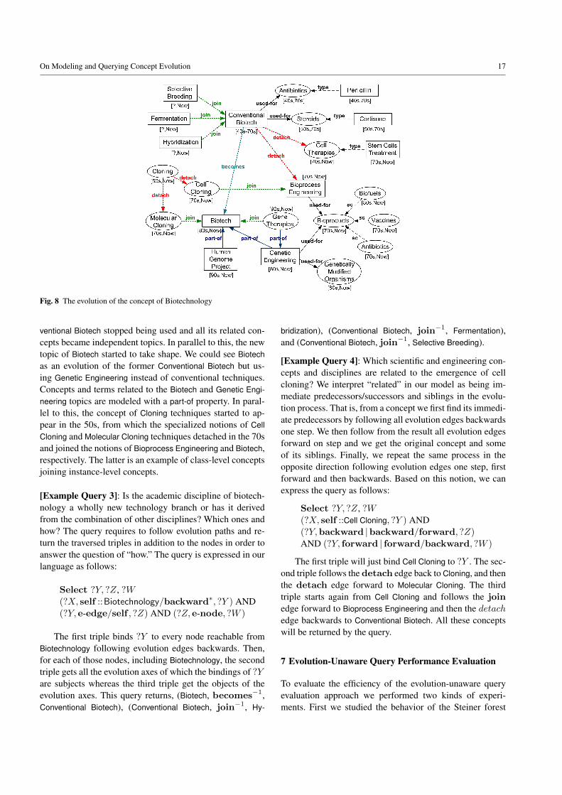
Consider now the evolution of the concept of biotechnol-ogy from a historical point of view. According to historians,biotechnology got its current meaning (related to molecularbiology) only after the 70s. Before that, the term biotechnol-ogy was used in areas as diverse as agriculture, microbiol-

ogy, and enzyme-based fermentation. Even though the term“biotechnology” was coined in 1919 by Karl Ereky, a Hun-garian engineer, the earliest mentions of biotechnology inthe news and specialized media refer to a set of ancient tech-niques like selective breeding, fermentation and hybridiza-tion. From the 70s the dominant meaning of biotechnologyhas been closely related to genetics. However, it is possibleto find news and other media articles from the 60s to the 80sthat use the term biotechnology to refer to an environmen-tally friendly technological orientation unrelated to geneticsbut closely related to bioprocess engineering. Not only theuse of the term changed from the 60s to the 90s, but also thetwo different meanings coexisted in the media for almosttwo decades.

Figure 8 illustrates the evolution of the notion of biotech-nology since the 40s. As in the previous example, classes inthe evolution base are represented by ovals and instancesby boxes. The used-for property is a normal property thatsimply links a technological concept to its products. The no-tions of Selective breeding, Fermentation and Hybridization ex-isted from an indeterminate time until now and in the 40sjoined the new topic of Conventional Biotech, which groupsancient techniques like the ones mentioned above. Over thenext decades, Conventional Biotech started to include moremodern therapies and products such as Cell Therapies, Peni-cillin and Cortisone. At some point in the 70s, the notionsof Cell Therapies and Bioprocess Engineering matured anddetached from Conventional Biotech becoming independentconcepts. Note that Cell Therapies is a class-level conceptthat detached from the an instance-level concept. The threeconcepts coexisted in time during part of the 70s, the lattertwo coexist even now. During the 70s, the notion of Con-

On Modeling and Querying Concept Evolution 17

Fig. 8 The evolution of the concept of Biotechnology

ventional Biotech stopped being used and all its related con-cepts became independent topics. In parallel to this, the newtopic of Biotech started to take shape. We could see Biotechas an evolution of the former Conventional Biotech but us-ing Genetic Engineering instead of conventional techniques.Concepts and terms related to the Biotech and Genetic Engi-neering topics are modeled with a part-of property. In paral-lel to this, the concept of Cloning techniques started to ap-pear in the 50s, from which the specialized notions of CellCloning and Molecular Cloning techniques detached in the 70sand joined the notions of Bioprocess Engineering and Biotech,respectively. The latter is an example of class-level conceptsjoining instance-level concepts.

[Example Query 3]: Is the academic discipline of biotech-nology a wholly new technology branch or has it derivedfrom the combination of other disciplines? Which ones andhow? The query requires to follow evolution paths and re-turn the traversed triples in addition to the nodes in order toanswer the question of “how.” The query is expressed in ourlanguage as follows:

Select ?Y, ?Z, ?W(?X, self ::Biotechnology/backward∗, ?Y ) AND(?Y, e-edge/self , ?Z) AND (?Z, e-node, ?W )

The first triple binds ?Y to every node reachable fromBiotechnology following evolution edges backwards. Then,for each of those nodes, including Biotechnology, the secondtriple gets all the evolution axes of which the bindings of ?Yare subjects whereas the third triple get the objects of theevolution axes. This query returns, (Biotech, becomes−1,Conventional Biotech), (Conventional Biotech, join−1, Hy-

bridization), (Conventional Biotech, join−1, Fermentation),and (Conventional Biotech, join−1, Selective Breeding).

[Example Query 4]: Which scientific and engineering con-cepts and disciplines are related to the emergence of cellcloning? We interpret “related” in our model as being im-mediate predecessors/successors and siblings in the evolu-tion process. That is, from a concept we first find its immedi-ate predecessors by following all evolution edges backwardsone step. We then follow from the result all evolution edgesforward on step and we get the original concept and someof its siblings. Finally, we repeat the same process in theopposite direction following evolution edges one step, firstforward and then backwards. Based on this notion, we canexpress the query as follows:

Select ?Y, ?Z, ?W(?X, self ::Cell Cloning, ?Y ) AND(?Y,backward |backward/forward, ?Z)

AND (?Y, forward | forward/backward, ?W )

The first triple will just bind Cell Cloning to ?Y . The sec-ond triple follows the detach edge back to Cloning, and thenthe detach edge forward to Molecular Cloning. The thirdtriple starts again from Cell Cloning and follows the join

edge forward to Bioprocess Engineering and then the detachedge backwards to Conventional Biotech. All these conceptswill be returned by the query.

7 Evolution-Unaware Query Performance Evaluation

To evaluate the efficiency of the evolution-unaware queryevaluation approach we performed two kinds of experi-ments. First we studied the behavior of the Steiner forest

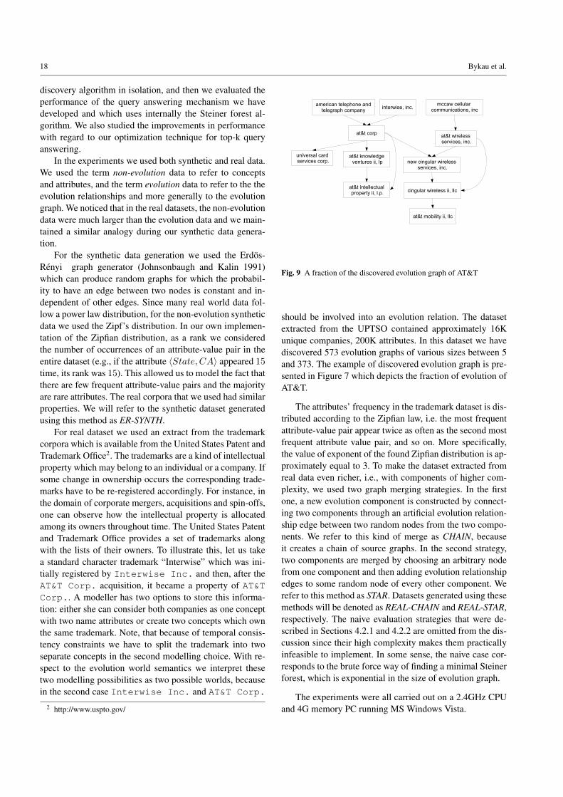
18 Bykau et al.

discovery algorithm in isolation, and then we evaluated theperformance of the query answering mechanism we havedeveloped and which uses internally the Steiner forest al-gorithm. We also studied the improvements in performancewith regard to our optimization technique for top-k queryanswering.

In the experiments we used both synthetic and real data.We used the term non-evolution data to refer to conceptsand attributes, and the term evolution data to refer to the theevolution relationships and more generally to the evolutiongraph. We noticed that in the real datasets, the non-evolutiondata were much larger than the evolution data and we main-tained a similar analogy during our synthetic data genera-tion.

For the synthetic data generation we used the Erdos-Renyi graph generator (Johnsonbaugh and Kalin 1991)which can produce random graphs for which the probabil-ity to have an edge between two nodes is constant and in-dependent of other edges. Since many real world data fol-low a power law distribution, for the non-evolution syntheticdata we used the Zipf’s distribution. In our own implemen-tation of the Zipfian distribution, as a rank we consideredthe number of occurrences of an attribute-value pair in theentire dataset (e.g., if the attribute 〈State, CA〉 appeared 15

time, its rank was 15). This allowed us to model the fact thatthere are few frequent attribute-value pairs and the majorityare rare attributes. The real corpora that we used had similarproperties. We will refer to the synthetic dataset generatedusing this method as ER-SYNTH.

For real dataset we used an extract from the trademarkcorpora which is available from the United States Patent andTrademark Office2. The trademarks are a kind of intellectualproperty which may belong to an individual or a company. Ifsome change in ownership occurs the corresponding trade-marks have to be re-registered accordingly. For instance, inthe domain of corporate mergers, acquisitions and spin-offs,one can observe how the intellectual property is allocatedamong its owners throughout time. The United States Patentand Trademark Office provides a set of trademarks alongwith the lists of their owners. To illustrate this, let us takea standard character trademark “Interwise” which was ini-tially registered by Interwise Inc. and then, after theAT&T Corp. acquisition, it became a property of AT&TCorp.. A modeller has two options to store this informa-tion: either she can consider both companies as one conceptwith two name attributes or create two concepts which ownthe same trademark. Note, that because of temporal consis-tency constraints we have to split the trademark into twoseparate concepts in the second modelling choice. With re-spect to the evolution world semantics we interpret thesetwo modelling possibilities as two possible worlds, becausein the second case Interwise Inc. and AT&T Corp.

2 http://www.uspto.gov/

Fig. 9 A fraction of the discovered evolution graph of AT&T

should be involved into an evolution relation. The datasetextracted from the UPTSO contained approximately 16Kunique companies, 200K attributes. In this dataset we havediscovered 573 evolution graphs of various sizes between 5and 373. The example of discovered evolution graph is pre-sented in Figure 7 which depicts the fraction of evolution ofAT&T.

The attributes’ frequency in the trademark dataset is dis-tributed according to the Zipfian law, i.e. the most frequentattribute-value pair appear twice as often as the second mostfrequent attribute value pair, and so on. More specifically,the value of exponent of the found Zipfian distribution is ap-proximately equal to 3. To make the dataset extracted fromreal data even richer, i.e., with components of higher com-plexity, we used two graph merging strategies. In the firstone, a new evolution component is constructed by connect-ing two components through an artificial evolution relation-ship edge between two random nodes from the two compo-nents. We refer to this kind of merge as CHAIN, becauseit creates a chain of source graphs. In the second strategy,two components are merged by choosing an arbitrary nodefrom one component and then adding evolution relationshipedges to some random node of every other component. Werefer to this method as STAR. Datasets generated using thesemethods will be denoted as REAL-CHAIN and REAL-STAR,respectively. The naive evaluation strategies that were de-scribed in Sections 4.2.1 and 4.2.2 are omitted from the dis-cussion since their high complexity makes them practicallyinfeasible to implement. In some sense, the naive case cor-responds to the brute force way of finding a minimal Steinerforest, which is exponential in the size of evolution graph.

The experiments were all carried out on a 2.4GHz CPUand 4G memory PC running MS Windows Vista.

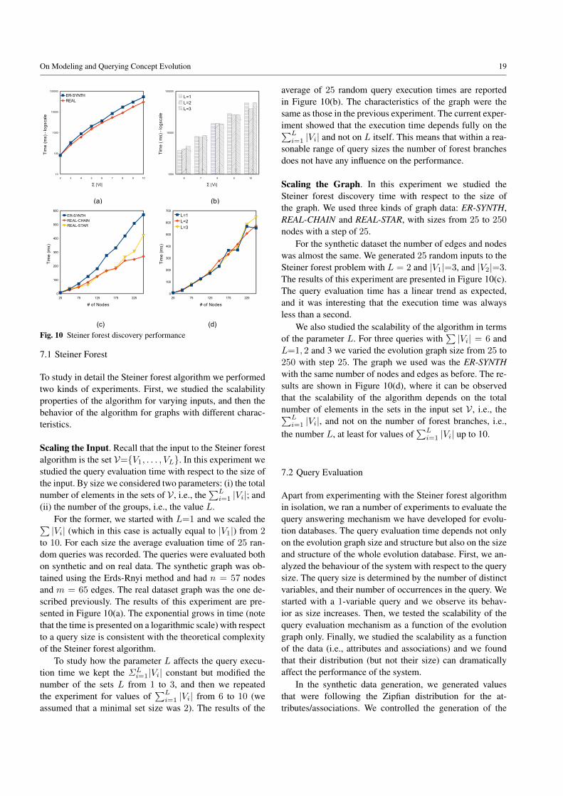
On Modeling and Querying Concept Evolution 19

Fig. 10 Steiner forest discovery performance

7.1 Steiner Forest

To study in detail the Steiner forest algorithm we performedtwo kinds of experiments. First, we studied the scalabilityproperties of the algorithm for varying inputs, and then thebehavior of the algorithm for graphs with different charac-teristics.

Scaling the Input. Recall that the input to the Steiner forestalgorithm is the set V=V1, . . . , VL. In this experiment westudied the query evaluation time with respect to the size ofthe input. By size we considered two parameters: (i) the totalnumber of elements in the sets of V , i.e., the

∑Li=1 |Vi|; and

(ii) the number of the groups, i.e., the value L.For the former, we started with L=1 and we scaled the∑|Vi| (which in this case is actually equal to |V1|) from 2

to 10. For each size the average evaluation time of 25 ran-dom queries was recorded. The queries were evaluated bothon synthetic and on real data. The synthetic graph was ob-tained using the Erds-Rnyi method and had n = 57 nodesand m = 65 edges. The real dataset graph was the one de-scribed previously. The results of this experiment are pre-sented in Figure 10(a). The exponential grows in time (notethat the time is presented on a logarithmic scale) with respectto a query size is consistent with the theoretical complexityof the Steiner forest algorithm.

To study how the parameter L affects the query execu-tion time we kept the ΣL

i=1|Vi| constant but modified thenumber of the sets L from 1 to 3, and then we repeatedthe experiment for values of

∑Li=1 |Vi| from 6 to 10 (we

assumed that a minimal set size was 2). The results of the

average of 25 random query execution times are reportedin Figure 10(b). The characteristics of the graph were thesame as those in the previous experiment. The current exper-iment showed that the execution time depends fully on the∑Li=1 |Vi| and not on L itself. This means that within a rea-

sonable range of query sizes the number of forest branchesdoes not have any influence on the performance.

Scaling the Graph. In this experiment we studied theSteiner forest discovery time with respect to the size ofthe graph. We used three kinds of graph data: ER-SYNTH,REAL-CHAIN and REAL-STAR, with sizes from 25 to 250

nodes with a step of 25.For the synthetic dataset the number of edges and nodes

was almost the same. We generated 25 random inputs to theSteiner forest problem with L = 2 and |V1|=3, and |V2|=3.The results of this experiment are presented in Figure 10(c).The query evaluation time has a linear trend as expected,and it was interesting that the execution time was alwaysless than a second.

We also studied the scalability of the algorithm in termsof the parameter L. For three queries with

∑|Vi| = 6 and

L=1, 2 and 3 we varied the evolution graph size from 25 to250 with step 25. The graph we used was the ER-SYNTHwith the same number of nodes and edges as before. The re-sults are shown in Figure 10(d), where it can be observedthat the scalability of the algorithm depends on the totalnumber of elements in the sets in the input set V , i.e., the∑Li=1 |Vi|, and not on the number of forest branches, i.e.,

the number L, at least for values of∑Li=1 |Vi| up to 10.

7.2 Query Evaluation

Apart from experimenting with the Steiner forest algorithmin isolation, we ran a number of experiments to evaluate thequery answering mechanism we have developed for evolu-tion databases. The query evaluation time depends not onlyon the evolution graph size and structure but also on the sizeand structure of the whole evolution database. First, we an-alyzed the behaviour of the system with respect to the querysize. The query size is determined by the number of distinctvariables, and their number of occurrences in the query. Westarted with a 1-variable query and we observe its behav-ior as size increases. Then, we tested the scalability of thequery evaluation mechanism as a function of the evolutiongraph only. Finally, we studied the scalability as a functionof the data (i.e., attributes and associations) and we foundthat their distribution (but not their size) can dramaticallyaffect the performance of the system.

In the synthetic data generation, we generated valuesthat were following the Zipfian distribution for the at-tributes/associations. We controlled the generation of the

20 Bykau et al.

Fig. 11 Query evaluation performance

ER-SYNTH dataset through four parameters, and in particu-lar, the pool of concepts, the exponent that is used to adjustthe steepness of the Zipfian distribution, the number of ele-ments that describes the maximum frequency of an attributeor association, and the number of attributes.The values ofthe parameters for the synthetic data are chosen to coincidewith those of the real corpora.

Scaling the Query. We considered a number of 1-variablequeries with a body of the form:

$x(attr1:value1), . . . , $x(attrN :valueN )

and we performed a number of experiments for different val-ues of N , i.e., the number of atoms in the query. For ev-ery atom we randomly chose an attribute-value pair froma pool of available distinct attribute name/value pairs. TheER-SYNTH graph that was generated had 57 nodes and 65

edges. The results are shown in Figure 11(a). The same fig-ure includes the results of the query evaluation on the realdataset that had a size similar to the synthetic. For the gen-eration of their non-evolution data we had the exponent setto 3, the number of elements parameter set to 15 and theirtotal number was 537. The results of the Figure 11(a) arein a logarithmic scale and confirm the expectation that thequery evaluation time is growing exponentially as the num-ber of variables in the query grows. If we compare theseresults with those of the Steiner forest algorithm for the re-spective case, it follows that the integrated system adds anotable overhead on top of the Steiner forest algorithm ex-ecution time. This is was due to the number of coalescencecandidates and the number of Steiner forests that needed to

be computed in order to obtain the cost of the elements inthe answer set. Although the parameters for the generationof the synthetic and real data coincided, their trends weredifferent, as Figure 11(c) illustrates.

We further tested how the number of concept variablesin the query affect the performance. Note that we are mainlyinterested in the concept-bound variables. Let M representthe number of distinct concept-bound variables in the query,and Mi the number of appearances of the i-th variable inthe query. Note that the number of distinct variables willrequire to solve a Steiner forest problem in which the inputV=V1, . . . , VL will have L=M and |Vi|=Mi, for eachi=1..M . The total number of variable appearances in thequery will naturally be

∑Mi=1Mi.

In the experiment, we chose a constant value for the∑Mi=1Mi and we run queries for M=1, 2 or 3. As a dataset

we used the ER-SYNTH with 57 nodes and 65 edges. 537 at-tributes were generated with the exponent parameter havingthe value 3 and the number of elements parameter to havethe value 15.A total of 53 synthetic associations were alsogenerated with the exponent parameter having the value 3,and the number of elements parameter to have the value 10.We used 25 randomly generated queries for each of the 3M values, and took their average execution time. We didmultiple runs of the above experiments for different valuesof

∑Mi=1Mi between 4 and 10. The outcome of the ex-

periments is shown in Figure 11(b) in a logarithmic scale.Clearly, the number of branches in a forest did not affectthe query evaluation time, i.e., queries with many variablesshowed the same increase in time as the 1-variable query forthe same

∑Mi=1Mi. Scaling the Data. In this experiment

we examined the query evaluation time with respect to thesize of the evolution graph. As evolution data, we used bothreal and synthetic sources. Regarding the real data, we useda series of graphs (and their attributes as non-evolution data)with sizes from 25 to 250 with step 25. The number of edgeswas 110% of the number of nodes for all graphs. For thereal dataset we used both the REAL-CHAIN and the REAL-STAR data. For each graph we generated 25 random querieswith 3 distinct variables, i.e., M=3, and each variable hadM1=2, M2=2 and M3=3 appearances in the query, and wemeasured the average time required to evaluate them. As asynthetic dataset the ER-SYNTH was used, generated to bethe same size as before but with the following Zipfian distri-bution parameters: exponent 3, number of elements 15 andnumber attributes 10 times more than the number of nodes.Note that we did not generate associations because the trade-mark dataset did not have any association that we could useas a guide. Figure 11(c) depicts the results of this experi-ment. It shows that there is a linear growth of time which isis accompanied with an increasing oscillations which can beexplained by the growing exponent of non-evolution data,

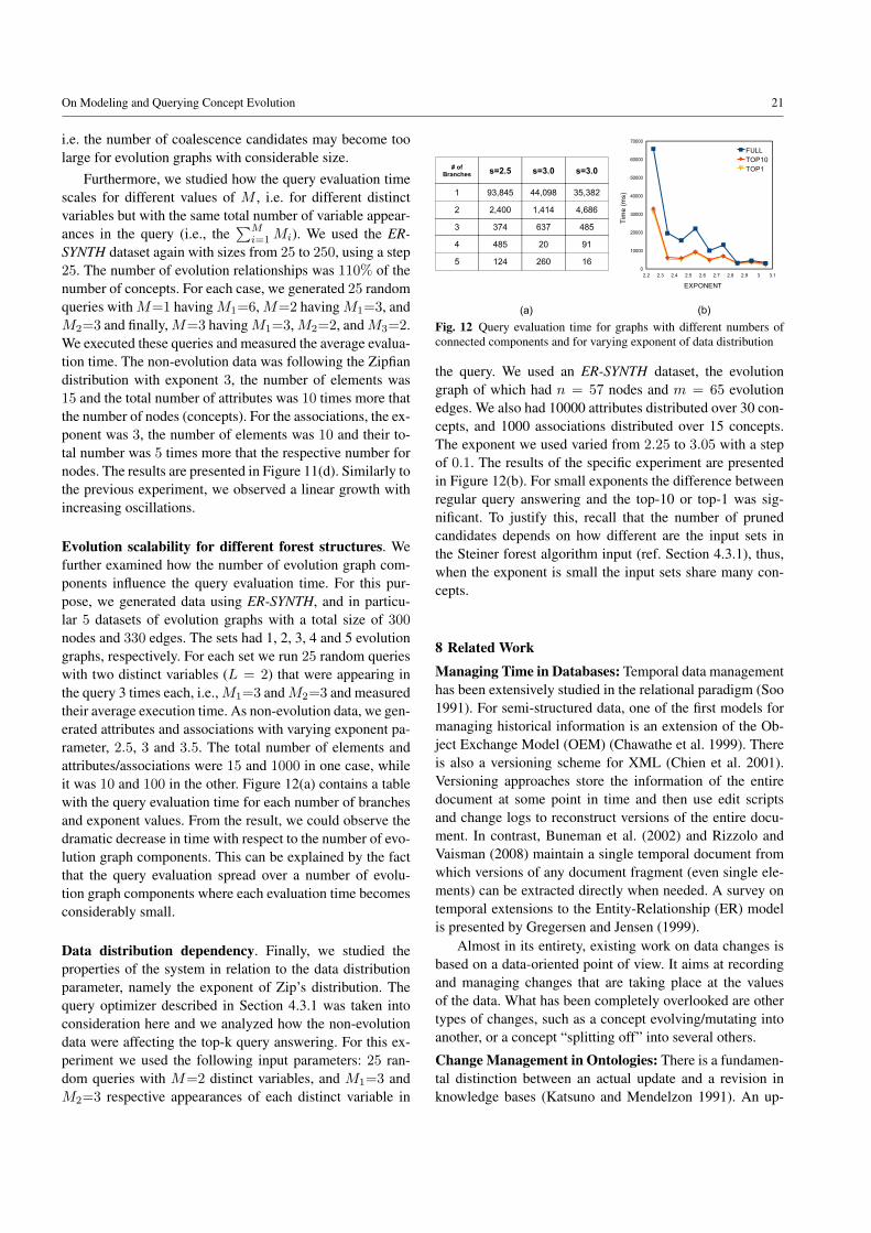
On Modeling and Querying Concept Evolution 21

i.e. the number of coalescence candidates may become toolarge for evolution graphs with considerable size.

Furthermore, we studied how the query evaluation timescales for different values of M , i.e. for different distinctvariables but with the same total number of variable appear-ances in the query (i.e., the

∑Mi=1Mi). We used the ER-

SYNTH dataset again with sizes from 25 to 250, using a step25. The number of evolution relationships was 110% of thenumber of concepts. For each case, we generated 25 randomqueries withM=1 havingM1=6,M=2 havingM1=3, andM2=3 and finally,M=3 havingM1=3,M2=2, andM3=2.We executed these queries and measured the average evalua-tion time. The non-evolution data was following the Zipfiandistribution with exponent 3, the number of elements was15 and the total number of attributes was 10 times more thatthe number of nodes (concepts). For the associations, the ex-ponent was 3, the number of elements was 10 and their to-tal number was 5 times more that the respective number fornodes. The results are presented in Figure 11(d). Similarly tothe previous experiment, we observed a linear growth withincreasing oscillations.

Evolution scalability for different forest structures. Wefurther examined how the number of evolution graph com-ponents influence the query evaluation time. For this pur-pose, we generated data using ER-SYNTH, and in particu-lar 5 datasets of evolution graphs with a total size of 300

nodes and 330 edges. The sets had 1, 2, 3, 4 and 5 evolutiongraphs, respectively. For each set we run 25 random querieswith two distinct variables (L = 2) that were appearing inthe query 3 times each, i.e.,M1=3 andM2=3 and measuredtheir average execution time. As non-evolution data, we gen-erated attributes and associations with varying exponent pa-rameter, 2.5, 3 and 3.5. The total number of elements andattributes/associations were 15 and 1000 in one case, whileit was 10 and 100 in the other. Figure 12(a) contains a tablewith the query evaluation time for each number of branchesand exponent values. From the result, we could observe thedramatic decrease in time with respect to the number of evo-lution graph components. This can be explained by the factthat the query evaluation spread over a number of evolu-tion graph components where each evaluation time becomesconsiderably small.

Data distribution dependency. Finally, we studied theproperties of the system in relation to the data distributionparameter, namely the exponent of Zip’s distribution. Thequery optimizer described in Section 4.3.1 was taken intoconsideration here and we analyzed how the non-evolutiondata were affecting the top-k query answering. For this ex-periment we used the following input parameters: 25 ran-dom queries with M=2 distinct variables, and M1=3 andM2=3 respective appearances of each distinct variable in

Fig. 12 Query evaluation time for graphs with different numbers ofconnected components and for varying exponent of data distribution

the query. We used an ER-SYNTH dataset, the evolutiongraph of which had n = 57 nodes and m = 65 evolutionedges. We also had 10000 attributes distributed over 30 con-cepts, and 1000 associations distributed over 15 concepts.The exponent we used varied from 2.25 to 3.05 with a stepof 0.1. The results of the specific experiment are presentedin Figure 12(b). For small exponents the difference betweenregular query answering and the top-10 or top-1 was sig-nificant. To justify this, recall that the number of prunedcandidates depends on how different are the input sets inthe Steiner forest algorithm input (ref. Section 4.3.1), thus,when the exponent is small the input sets share many con-cepts.

8 Related WorkManaging Time in Databases: Temporal data managementhas been extensively studied in the relational paradigm (Soo1991). For semi-structured data, one of the first models formanaging historical information is an extension of the Ob-ject Exchange Model (OEM) (Chawathe et al. 1999). Thereis also a versioning scheme for XML (Chien et al. 2001).Versioning approaches store the information of the entiredocument at some point in time and then use edit scriptsand change logs to reconstruct versions of the entire docu-ment. In contrast, Buneman et al. (2002) and Rizzolo andVaisman (2008) maintain a single temporal document fromwhich versions of any document fragment (even single ele-ments) can be extracted directly when needed. A survey ontemporal extensions to the Entity-Relationship (ER) modelis presented by Gregersen and Jensen (1999).

Almost in its entirety, existing work on data changes isbased on a data-oriented point of view. It aims at recordingand managing changes that are taking place at the valuesof the data. What has been completely overlooked are othertypes of changes, such as a concept evolving/mutating intoanother, or a concept “splitting off” into several others.

Change Management in Ontologies: There is a fundamen-tal distinction between an actual update and a revision inknowledge bases (Katsuno and Mendelzon 1991). An up-

22 Bykau et al.

date brings the knowledge base up to date when the worldit models has changed. Our evolution framework modelsupdates since it describes how real-world concepts havechanged over time. In contrast, a revision incorporates newknowledge from a world that has not changed. An ap-proach to model revision in RDF ontologies has been pre-sented (Konstantinidis et al. 2007). The work on ontologyevolution in data integration (Kondylakis and Plexousakis2010) automatically finds ways to update mappings whenthe underlying ontologies were changed. In contrast to ourkind of evolution,(Kondylakis and Plexousakis 2010) con-siders structural changes of ontologies with the main focuson mapping recomputation. The survey (Flouris et al. 2008)provides a thorough classification of the types of changesthat occur in ontologies. However, there is no entry in theirtaxonomy that corresponds to the kind of concept evolu-tion we developed in this work; in fact, they view evolutionas a special case of versioning. Similarly to versioning indatabases, ontology versioning study the problem of main-taining changes in ontologies by creating and managing dif-ferent variants of it (Klein and Fensel 2001). In our case,we focus on the evolution of a concept that spans differ-ent concepts (e.g., student to professor, research lab to in-dependent corporate concept). Highly related, yet different,to concept evolution is the problem of terminology evolu-tion that studies how terms describing the same notion ina domain of discourse are changing over time (Tahmasebiet al. 2008). The high-level changes in RDF/S knowledgebases (Papavassiliou et al. 2009) represent similar to ourevolution operators ideas. However, our work focuses onthis kind of changes and elaborates on their properties andquery evaluation strategies. Closer to our work is the pro-posal (Kauppinen and Hyvonen 2007) for modeling changesin geographical information systems (GIS). They use the no-tion of a change bridge to model how the area of geographi-cal concept (countries, provinces) evolve. A change bridge isassociated with a change point and indicates what conceptsbecome obsolete, what new concepts are created, and howthe new concepts overlap with older ones. Since they focuson the GIS domain, they are not able to model causality andtypes of evolution involving abstract concepts beyond geo-graphical concepts.

9 ConclusionThis work studies the problem of concept evolution. In con-trast to temporal models and schema evolution, concept evo-lution deals with mereological and causal relationships be-tween concepts. Recording concept evolution also enablesusers to pose queries on the history of a concept.

We present a framework for modeling evolution as anextension of temporal RDF with mereology and causal prop-erties. These properties are expressed with a set of evolutionterms and its query language is an extension of nSPARQL

that allows navigation over the history of the concepts. Fur-thermore, we have designed and implemented an evaluationtechnique that allows query answering over databases wherethe evolution model that the user has in mind is of differentgranularity than the one used in the database. The solutionrequired the computation of a Steiner forest. For the later wehave presented a novel algorithm for computing its optimalsolution. Finally, we have studied two real use cases wherewe show the applicability of the proposed framework. In ad-dition, we have performed a number of an extensive experi-mental evaluation to determine the efficiency of the evalua-tion technique in the case for evolution-unaware queries.

As future work, we plan to investigate possible algorith-mic improvements for the Steiner forest algorithm by par-allelization and approximization. Moreover, we look intoother non-temporal domains where we could leverage theevolution (casual) relationships.

References

Bhalotia, Gaurav, Arvind Hulgeri, Charuta Nakhe, SoumenChakrabarti, and S. Sudarshan (2002), “Keyword search-ing and browsing in databases using banks.” In ICDE,431–440.

Blakeley, J., P. A. Larson, and F. W. Tompa (1986), “Effi-ciently Updating Materialized Views.” In SIGMOD, 61–71.

Buneman, P., S. Khanna, K Tajima, and W. Tan (2002),“Archiving scientific data.” In SIGMOD, 1–12.

Bykau, Siarhei, John Mylopoulos, Flavio Rizzolo, andYannis Velegrakis (2011), “Supporting queries spanningacross phases of evolving artifacts using steiner forests.”In CIKM, 1649–1658.

Chawathe, S., S. Abiteboul, and J. Widom (1999), “Manag-ing historical semistructured data.” In Theory and Prac-tice of Object Systems, 143–162.

Chien, S., V. Tsotras, and C. Zaniolo (2001), “Efficient man-agement of multiversion documents by object referenc-ing.” In VLDB, 291–300.

Dalvi, N. N., R. Kumar, B. Pang, R. Ramakrishnan,A. Tomkins, P. Bohannon, S. Keerthi, and S. Merugu(2009), “A web of concepts.” In PODS, 1–12.

Dalvi, Nilesh and Dan Suciu (2007), “Efficient query evalu-ation on probabilistic databases.” The VLDB Journal, 16,523–544.

Ding, Bolin, J Xu Yu, Shan Wang, Lu Qin, Xiao Zhang, andXuemin Lin (2007), “Finding Top-k Min-Cost ConnectedTrees in Databases.” ICDE, 836–845.

Dong, X., A. Y. Halevy, and J. Madhavan (2005), “Refer-ence Reconciliation in Complex Information Spaces.” InSIGMOD, 85–96.

On Modeling and Querying Concept Evolution 23

Dreyfus, S E and R A Wagner (1972), “The Steiner problemin graphs.” Networks, 1, 195–207.

Dyreson, Curtis E., William S. Evans, Hong Lin, andRichard T. Snodgrass (2000), “Efficiently supported tem-poral granularities.” IEEE Trans. Knowl. Data Eng., 12,568–587.

Flouris, Giorgos, Dimitris Manakanatas, Haridimos Kondy-lakis, Dimitris Plexousakis, and Grigoris Antoniou(2008), “Ontology change: classification and survey.”Knowledge Eng. Review, 23, 117–152.

Gassner, Elisabeth (2010), “The Steiner Forest Problem re-visited.” Journal of Discrete Algorithms, 8, 154–163.

Gregersen, Heidi and Christian S. Jensen (1999), “Tempo-ral Entity-Relationship models - a survey.” IEEE Trans.Knowl. Data Eng., 11, 464–497.

Gutierrez, Claudio, Carlos A. Hurtado, and Alejandro A.Vaisman (2005), “Temporal RDF.” In ESWC, 93–107.

He, Hao, Haixun Wang, Jun Yang 0001, and Philip S. Yu(2007), “Blinks: ranked keyword searches on graphs.” InSIGMOD Conference, 305–316.

Hull, R. and M. Yoshikawa (1990), “ILOG: Declarative Cre-ation and Manipulation of Object Identifiers.” In VLDB,455–468.

Johnsonbaugh, Richard and Martin Kalin (1991), “A graphgeneration software package.” In SIGCSE, 151–154.

Kacholia, Varun, Shashank Pandit, Soumen Chakrabarti,S. Sudarshan, Rushi Desai, and Hrishikesh Karambelkar(2005), “Bidirectional expansion for keyword search ongraph databases.” In VLDB, 505–516.

Katsuno, Hirofumi and Alberto O. Mendelzon (1991), “Onthe difference between updating a knowledge base andrevising it.” In KR, 387–394.

Kauppinen, Tomi and Eero Hyvonen (2007), “Modeling andreasoning about changes in ontology time series.” In On-tologies: A Handbook of Principles, Concepts and Appli-cations in Information Systems, 319–338.

Keet, C. Maria and Alessandro Artale (2008), “Representingand reasoning over a taxonomy of part-whole relations.”Applied Ontology, 3, 91–110.

Kimelfeld, B. and Y. Sagiv (2006), “New algorithms forcomputing steiner trees for a fixed number of terminals.”Http://www.cs.huji.ac.il/ bennyk/papers/steiner06.pdf.

Klein, Michel C. A. and Dieter Fensel (2001), “Ontologyversioning on the semantic web.” In SWWS, 75–91.

Kondylakis, Haridimos and Dimitris Plexousakis (2010),“Enabling ontology evolution in data integration.” In Pro-ceedings of the 2010 EDBT/ICDT Workshops, EDBT ’10,38:1–38:7, ACM, New York, NY, USA.

Konstantinidis, George, Giorgos Flouris, Grigoris Antoniou,and Vassilis Christophides (2007), “On RDF/S ontologyevolution.” In SWDB-ODBIS, 21–42.

Lenzerini, M. (2002), “Data Integration: A Theoretical Per-spective.” In PODS, 233–246.

Lerner, B. S. (2000), “A Model for Compound TypeChanges Encountered in Schema Evolution.” TODS, 25,83–127.

Palpanas, T., J. Chaudhry, P. Andritsos, and Y. Vele-grakis (2008), “Entity Data Management in OKKAM.”In SWAP, 729–733.

Papavassiliou, Vicky, Giorgos Flouris, Irini Fundulaki, Dim-itris Kotzinos, and Vassilis Christophides (2009), “On de-tecting high-level changes in rdf/s kbs.” In ISWC, 473–488.

Perez, Jorge, Marcelo Arenas, and Claudio Gutierrez(2008), “nSPARQL: A navigational language for RDF.”In ISWC, 66–81.

Rizzolo, F. and A. A. Vaisman (2008), “Temporal XML:modeling, indexing, and query processing.” VLDBJ, 17,1179–1212.

Rizzolo, F., Y. Velegrakis, J. Mylopoulos, and S. Bykau(2009), “Modeling Concept Evolution: A Historical Per-spective.” In ER, 331–345.

Soo, M. D. (1991), “Bibliography on Temporal Databases.”SIGMODREC, 20, 14–23.

Tahmasebi, Nina, Tereza Iofciu, Thomas Risse, ClaudiaNiederee, and Wolf Siberski (2008), “Terminology evolu-tion in web archiving: Open issues.” In International WebArchiving Workshop.

Velegrakis, Yannis, Renee J. Miller, and Lucian Popa(2004), “Preserving mapping consistency under schemachanges.” VLDB J., 13, 274–293.

W3C (2004), “RDF vocabulary description language 1.0:RDF Schema.” Http://www.w3.org/TR/rdf-schema/.