Embed Size (px)
Citation preview
On Minimum- and Maximum-Weight Minimum Spanning Trees
with Neighborhoods
University of Waterloo Technical Report CS-2012-14
Reza Dorrigiv∗,1, Robert Fraser† ,2, Meng He‡,1, Shahin Kamali§ ,2, Akitoshi Kawamura¶,3,Alejandro Lopez-Ortiz∥,2, and Diego Seco∗∗,4
1Dalhousie University, Halifax, Canada2University of Waterloo, Waterloo, Ontario, Canada
3University of Tokyo, Tokyo, Japan4University of A Coruna, A Coruna, Spain
August 27, 2012
Abstract
We study optimization problems for the Euclidean minimum spanning tree (MST) on im-precise data. To model imprecision, we accept a set of disjoint disks in the plane as input. Fromeach member of the set, one point must be selected, and the MST is computed over the setof selected points. We consider both minimizing and maximizing the weight of the MST overthe input. The minimum weight version of the problem is known as the minimum spanningtree with neighborhoods (MSTN) problem, and the maximum weight version (max-MSTN)has not been studied previously to our knowledge. We provide deterministic and parameterizedapproximation algorithms for the max-MSTN problem, and a parameterized algorithm for theMSTN problem. Additionally, we present hardness of approximation proofs for both settings.
1 Introduction
We consider geometric problems dealing with imprecise data. In this setting, each point of theinput is provided as a region of uncertainty, i.e., a geometric object such as a line, disk, set ofpoints, etc., and the exact position of the point may be anywhere in the object. Each object isunderstood to represent the set of possible positions for the corresponding point. In our work, we
∗[email protected]†[email protected]‡[email protected]§[email protected]¶[email protected]∥[email protected]
1
study the Euclidean minimum spanning tree (MST) problem. Given a tree T , we define its weightw(T ) to be the sum of the weights of the edges in T . For a set of fixed points P in Euclidean space,the weight of an edge is the distance between the endpoints, and we write mst(P ) for the weightof the MST on P . Thus, mst(P ) = minw(T ), where the minimum is taken over all spanning treesT on P .
Given a set of disjoint disks as input, we wish to determine the minimum and maximum weightMSTs possible when a point is fixed in each disk. The minimum weight MST version of the problemhas been studied previously, and is known as the minimum spanning tree with neighborhoodsproblem (MSTN). This paper introduces the maximum weight MST version of the problem, whichwe call the max-MSTN problem. Assume we are given a set D = {D1, . . . , Dn} of disjoint disksin the plane, i.e., Di ∩Dj = ∅ if i = j. The MSTN problem on D asks for the selection of a pointpi ∈ Di for each Di ∈ D such that the weight of the MST of the selected points is minimized.Similarly, max-MSTN asks for a selection of pi such that the weight of the MST of the selectedpoints is maximized.
1.1 Related Work
The first known MST algorithm was published over 80 years ago [10], and a number of successfulvariants have followed (see [7] for the history of the problem). A review of models of uncertaintyand data imprecision for computational geometry problems is provided in [9]. Here, we discuss afew results that are directly related to the MST problem and our model of imprecision.
The MSTN problem on unit disks has been shown to admit a PTAS [13]. A hardness prooffor a generalization of MSTN where the neighborhoods are either disks or rectangles appeared in[13], but the proof was faulty. One of the authors later conjectured that a reduction from planar3-SAT might be used to show the hardness of the MSTN problem [12, p.106]. In Section 3.2, weprove this conjecture.
Loffler and van Kreveld [9] demonstrated that it is algebraically difficult to compute the MSTwhen the regions of uncertainty are continuous regions of the plane, even for very simple inputssuch as disks or squares, as the solution may involve the roots of high degree polynomials. It is ofindependent interest to see if the problem is combinatorially difficult. In the same paper, authorsproved that the MSTN problem is (combinatorially) NP-hard if the regions of uncertainty are notpairwise disjoint, through a reduction from the minimum Steiner tree problem. In this paper weprove the hardness of the special case in which the regions are pairwise disjoint.
Erlebach et al. [5] used a model of uncertainty where information regarding the weight of anedge between a pair of points or the position of a point may be obtained by pinging the edge orvertex, and they sought to minimize the number of pings required while obtaining the optimalsolution. The distinction is that in their work, they were interested in reducing the amount ofcommunication that is required to locate points within a region of uncertainty, while in our model,the objective is to optimize the MST given regions of uncertainty.
Researchers have considered other related problems that deal with imprecise data. The trav-elling salesman with neighborhoods (TSPN) problem has been studied extensively. The problemwas introduced by Arkin and Hassin [1], in a paper that has been applied, improved, built-uponor otherwise referenced over 150 times. There exists a PTAS for TSPN when the neighborhoodsare disjoint unit disks [4]. The most general version of the problem, where regions may overlap
2
and may have varying sizes, is known to be APX-hard [2]. The problem of maximizing the smallestpairwise distance in a set of n points with neighborhoods has also been studied and proved to beNP-hard [6].
1.2 Our Results
We present a variety of results related to theMSTN and max-MSTN problems. For both problemswe assume the regions of uncertainty (disks) are disjoint.
• max-MSTN: deterministic 1/2-approximation;
• max-MSTN: parameterized 1 − 2k+4 -approximation (where k represents the separability of
the instance, which is to be defined later);
• max-MSTN: proof of hardness of approximation;
• MSTN: parameterized 1 + 2/k-approximation (k is the separability of the instance);
• MSTN: proof of hardness of approximation.
The deterministic approximation algorithm for max-MSTN (Section 2.1) is based on choosingthe center points of the disks; the interesting aspect in this section lies in the analysis. Theparameterized algorithms (Sections 2.2 and 3.1) for both settings were inspired by the observationthat the approximation factor improves rapidly as the distance between disks increases. To addressthis, we introduce a measure of how much separation exists between the disks, which we callseparability, and we analyze the approximation factor of the MST on disk centers with respect toseparability.
For both hardness of approximation results, we establish that there is no FPTAS for the prob-lems unless P=NP. Although the hardness proofs both consist of reductions from planar 3-SAT,the gadgets used are quite distinct and either reduction is interesting even given the existence ofthe other. In both cases, we construct an instance of our problem from the planar 3-SAT instance,and show that it is possible to compute the weight of the optimal solution to our problem assumingthat the 3-SAT instance is satisfiable. If the instance is not satisfiable, we prove that the weightis changed by at least a constant amount (reduced by at least 0.33 units for max-MSTN, andincreased by at least 0.84 units for MSTN).
2 MAX-MSTN
In this section we study a couple of approximation algorithms for the max-MSTN problem, andthen we present the proof of hardness of approximation. We begin with a deterministic algorithmbelow, followed by a parameterized algorithm in Section 2.2.
2.1 Deterministic 1/2-Approximation Algorithm
To approximate the solution to max-MSTN, we first consider the algorithm that builds an MSTon the centers of the disks. We show this algorithm approximates the optimal solution within a
3
(a) (b) (c)
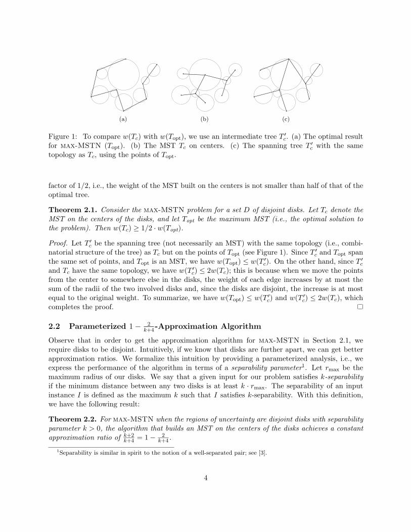
Figure 1: To compare w(Tc) with w(Topt), we use an intermediate tree T ′c. (a) The optimal result
for max-MSTN (Topt). (b) The MST Tc on centers. (c) The spanning tree T ′c with the same
topology as Tc, using the points of Topt.
factor of 1/2, i.e., the weight of the MST built on the centers is not smaller than half of that of theoptimal tree.
Theorem 2.1. Consider the max-MSTN problem for a set D of disjoint disks. Let Tc denote theMST on the centers of the disks, and let Topt be the maximum MST (i.e., the optimal solution tothe problem). Then w(Tc) ≥ 1/2 · w(Topt).
Proof. Let T ′c be the spanning tree (not necessarily an MST) with the same topology (i.e., combi-
natorial structure of the tree) as Tc but on the points of Topt (see Figure 1). Since T′c and Topt span
the same set of points, and Topt is an MST, we have w(Topt) ≤ w(T ′c). On the other hand, since T ′
c
and Tc have the same topology, we have w(T ′c) ≤ 2w(Tc); this is because when we move the points
from the center to somewhere else in the disks, the weight of each edge increases by at most thesum of the radii of the two involved disks and, since the disks are disjoint, the increase is at mostequal to the original weight. To summarize, we have w(Topt) ≤ w(T ′
c) and w(T ′c) ≤ 2w(Tc), which
completes the proof.
2.2 Parameterized 1− 2k+4
-Approximation Algorithm
Observe that in order to get the approximation algorithm for max-MSTN in Section 2.1, werequire disks to be disjoint. Intuitively, if we know that disks are further apart, we can get betterapproximation ratios. We formalize this intuition by providing a parameterized analysis, i.e., weexpress the performance of the algorithm in terms of a separability parameter1. Let rmax be themaximum radius of our disks. We say that a given input for our problem satisfies k-separabilityif the minimum distance between any two disks is at least k · rmax. The separability of an inputinstance I is defined as the maximum k such that I satisfies k-separability. With this definition,we have the following result:
Theorem 2.2. For max-MSTN when the regions of uncertainty are disjoint disks with separabilityparameter k > 0, the algorithm that builds an MST on the centers of the disks achieves a constantapproximation ratio of k+2
k+4 = 1− 2k+4 .
1Separability is similar in spirit to the notion of a well-separated pair; see [3].
4
Proof. Let Tc be the MST on the centers of the disks. We can extend the analysis in the proofof Theorem 1 to show that the approximation factor is k+2
k+4 = 1− 2k+4 for any input that satisfies
k-separability. Define Topt and T ′c as before. Consider an arbitrary edge e in T ′
c and let Di and Dj
be the two disks connected by e. Let ri and rj be the radii of Di and Dj , respectively, and let dbe the distance between Di and Dj . In Tc the disks Di and Dj are connected by an edge e′ whoseweight is d+ ri + rj . The weight of e, on the other hand, can be at most d+ 2ri + 2rj . Therefore,the ratio between the weight of an edge in Tc and its corresponding edge in T ′
c is at least
d+ ri + rjd+ 2ri + 2rj
≥ krmax + ri + rjkrmax + 2ri + 2rj
≥ krmax + rmax + rmax
krmax + 2rmax + 2rmax=
k + 2
k + 4.
Since this holds for any edge of T ′c, we get w(Tc) ≥ k+2
k+4w(T′c) ≥ k+2
k+4w(Topt), and we get an
approximation factor of k+2k+4 .
The approximation ratio gets arbitrarily close to 1 as k increases. This confirms our intuitionthat if the disks are further apart (more separate), we get a better approximation factor.
2.3 Hardness of Approximation
We present a hardness proof for the max-MSTN problem by a reduction from the planar 3-SATproblem [8]. Planar 3-SAT is a variant of 3-SAT in which the graph G = (V,E) associated withthe formula is planar.
Theorem 2.3. max-MSTN does not admit an FPTAS unless P=NP.
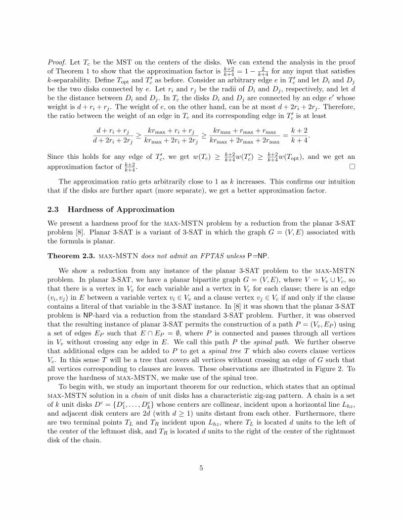
We show a reduction from any instance of the planar 3-SAT problem to the max-MSTNproblem. In planar 3-SAT, we have a planar bipartite graph G = (V,E), where V = Vv ∪ Vc, sothat there is a vertex in Vv for each variable and a vertex in Vc for each clause; there is an edge(vi, vj) in E between a variable vertex vi ∈ Vv and a clause vertex vj ∈ Vc if and only if the clausecontains a literal of that variable in the 3-SAT instance. In [8] it was shown that the planar 3-SATproblem is NP-hard via a reduction from the standard 3-SAT problem. Further, it was observedthat the resulting instance of planar 3-SAT permits the construction of a path P = (Vv, EP ) usinga set of edges EP such that E ∩ EP = ∅, where P is connected and passes through all verticesin Vv without crossing any edge in E. We call this path P the spinal path. We further observethat additional edges can be added to P to get a spinal tree T which also covers clause verticesVc. In this sense T will be a tree that covers all vertices without crossing an edge of G such thatall vertices corresponding to clauses are leaves. These observations are illustrated in Figure 2. Toprove the hardness of max-MSTN, we make use of the spinal tree.
To begin with, we study an important theorem for our reduction, which states that an optimalmax-MSTN solution in a chain of unit disks has a characteristic zig-zag pattern. A chain is a setof k unit disks Dc = {Dc
1, . . . , Dck} whose centers are collinear, incident upon a horizontal line Lhz,
and adjacent disk centers are 2d (with d ≥ 1) units distant from each other. Furthermore, thereare two terminal points TL and TR incident upon Lhz, where TL is located d units to the left ofthe center of the leftmost disk, and TR is located d units to the right of the center of the rightmostdisk of the chain.
5
(a) The reduction from 3-SAT to planar3-SAT.
(b) The planar gadget located in the intersec-tion points. Variable and clause vertices arerepresented by large and small circles, respec-tively.
Figure 2: The reduction from 3-SAT to planar 3-SAT as presented in [8]. The variable and clausevertices of 3-SAT are located respectively in x and y axis, and the edges are drawn as orthogonalpaths (a). A planar gadget is placed on each intersection point. Each gadget includes some newvariable and clause vertices (b). In [8], it is observed that there is a path (we call it the spinalpath) that covers all variable vertices of planar instance without crossing any edge (solid lines). Weobserve that additional edges can be added to the spinal path to obtain a tree (spinal tree) whichspans clause variables as leaves (dashed lines).
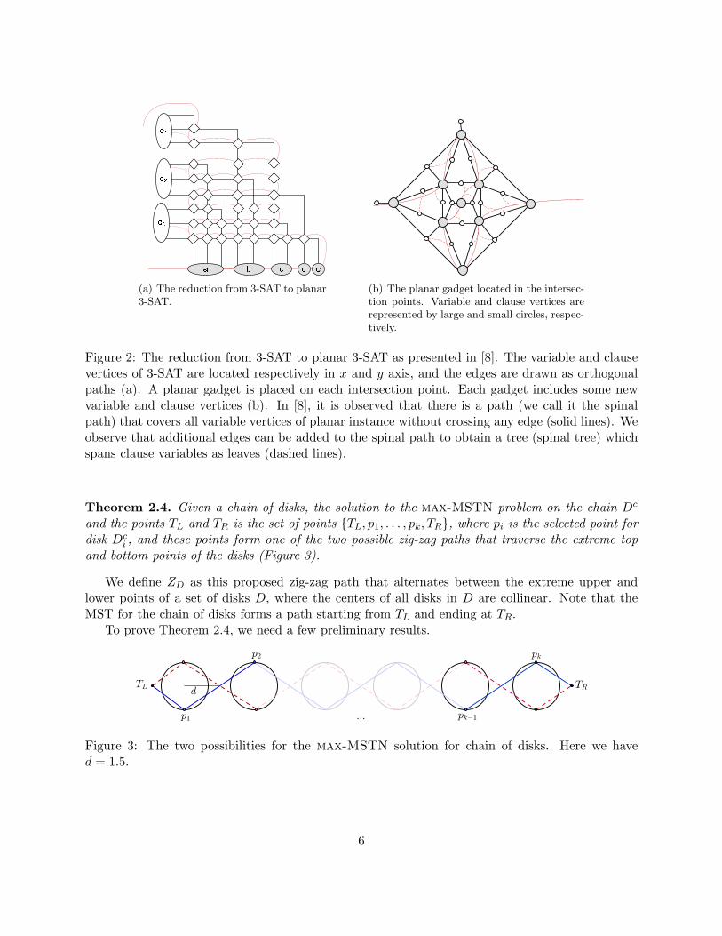
Theorem 2.4. Given a chain of disks, the solution to the max-MSTN problem on the chain Dc
and the points TL and TR is the set of points {TL, p1, . . . , pk, TR}, where pi is the selected point fordisk Dc
i , and these points form one of the two possible zig-zag paths that traverse the extreme topand bottom points of the disks (Figure 3).
We define ZD as this proposed zig-zag path that alternates between the extreme upper andlower points of a set of disks D, where the centers of all disks in D are collinear. Note that theMST for the chain of disks forms a path starting from TL and ending at TR.
To prove Theorem 2.4, we need a few preliminary results.
Figure 3: The two possibilities for the max-MSTN solution for chain of disks. Here we haved = 1.5.
6
Lemma 2.5. Given a disk, if the set of edges containing a point in the disk is fixed for any positionof the point, any max-MSTN solution does not contain a point inside the disk (i.e., the selectedpoint is on the circumference of the disk).
Proof. Suppose we are given a point p in a disk D, and a set of points Q, |Q| ≥ 1, where thereexists an edge between p and each point in Q. Given any line ℓ where p ∈ ℓ, let p′ be a point onℓ ∩ D. Let w be the sum of the weights of edges between p′ and each point in Q. The weight ofeach edge (as p′ runs along ℓ) is a convex function, and therefore so is the sum w [11]. Hence, thesum of the weights of the edges is maximized at one of the two intersection points of ℓ with D.
The following lemma states that a max-MSTN solution should follow the path of a ray of lightwhich is started at point TL and is reflected on the intersection with each disk.
Lemma 2.6. Let p1 be the selected point of a max-MSTN solution on the leftmost disk in a chain.Consider the segment Lp1 as a ray of light that is reflected on the interior face of each disk. Anyvalid max-MSTN solution follows the path traversed by the ray, i.e., the two neighboring segmentsof the MST are the reflection of each other on the tangent line of the intersection point.
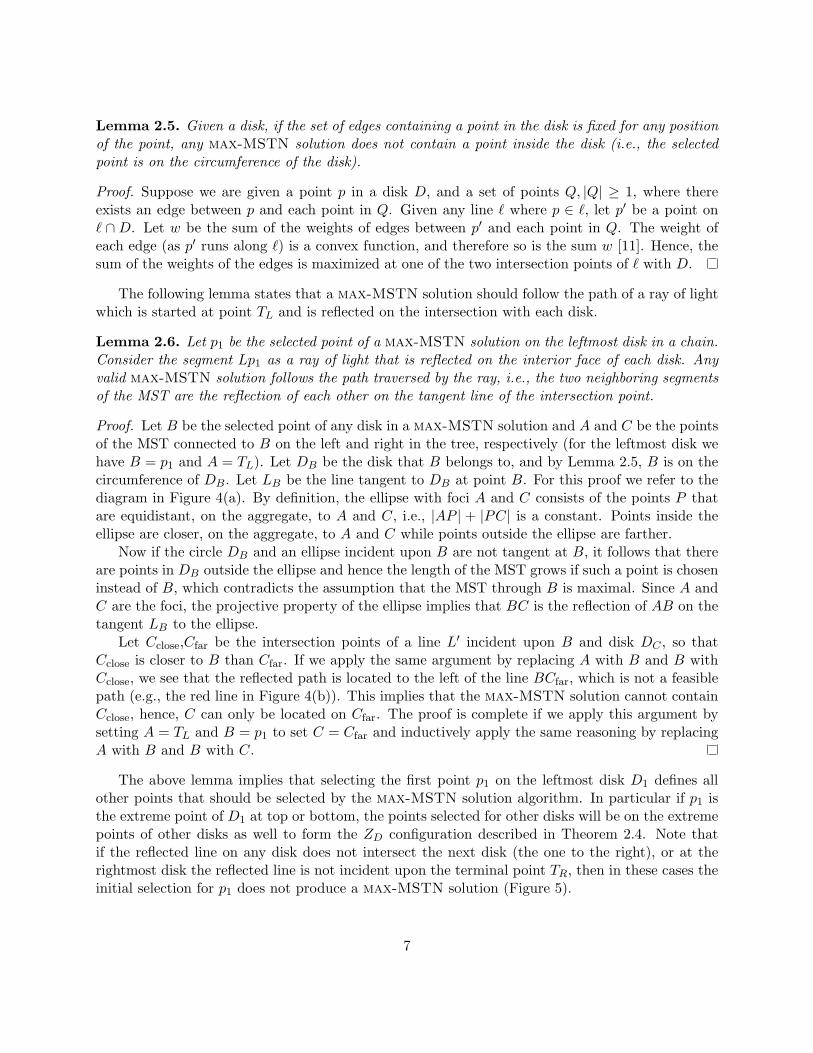
Proof. Let B be the selected point of any disk in a max-MSTN solution and A and C be the pointsof the MST connected to B on the left and right in the tree, respectively (for the leftmost disk wehave B = p1 and A = TL). Let DB be the disk that B belongs to, and by Lemma 2.5, B is on thecircumference of DB. Let LB be the line tangent to DB at point B. For this proof we refer to thediagram in Figure 4(a). By definition, the ellipse with foci A and C consists of the points P thatare equidistant, on the aggregate, to A and C, i.e., |AP | + |PC| is a constant. Points inside theellipse are closer, on the aggregate, to A and C while points outside the ellipse are farther.
Now if the circle DB and an ellipse incident upon B are not tangent at B, it follows that thereare points in DB outside the ellipse and hence the length of the MST grows if such a point is choseninstead of B, which contradicts the assumption that the MST through B is maximal. Since A andC are the foci, the projective property of the ellipse implies that BC is the reflection of AB on thetangent LB to the ellipse.
Let Cclose,Cfar be the intersection points of a line L′ incident upon B and disk DC , so thatCclose is closer to B than Cfar. If we apply the same argument by replacing A with B and B withCclose, we see that the reflected path is located to the left of the line BCfar, which is not a feasiblepath (e.g., the red line in Figure 4(b)). This implies that the max-MSTN solution cannot containCclose, hence, C can only be located on Cfar. The proof is complete if we apply this argument bysetting A = TL and B = p1 to set C = Cfar and inductively apply the same reasoning by replacingA with B and B with C.
The above lemma implies that selecting the first point p1 on the leftmost disk D1 defines allother points that should be selected by the max-MSTN solution algorithm. In particular if p1 isthe extreme point of D1 at top or bottom, the points selected for other disks will be on the extremepoints of other disks as well to form the ZD configuration described in Theorem 2.4. Note thatif the reflected line on any disk does not intersect the next disk (the one to the right), or at therightmost disk the reflected line is not incident upon the terminal point TR, then in these cases theinitial selection for p1 does not produce a max-MSTN solution (Figure 5).
7
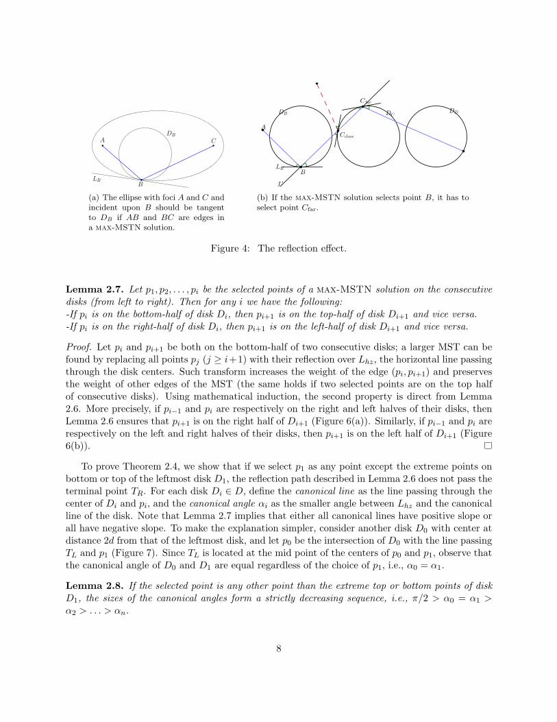
A C
B
DB
LB
(a) The ellipse with foci A and C andincident upon B should be tangentto DB if AB and BC are edges ina max-MSTN solution.
(b) If the max-MSTN solution selects point B, it has toselect point Cfar.
Figure 4: The reflection effect.
Lemma 2.7. Let p1, p2, . . . , pi be the selected points of a max-MSTN solution on the consecutivedisks (from left to right). Then for any i we have the following:-If pi is on the bottom-half of disk Di, then pi+1 is on the top-half of disk Di+1 and vice versa.-If pi is on the right-half of disk Di, then pi+1 is on the left-half of disk Di+1 and vice versa.
Proof. Let pi and pi+1 be both on the bottom-half of two consecutive disks; a larger MST can befound by replacing all points pj (j ≥ i+1) with their reflection over Lhz, the horizontal line passingthrough the disk centers. Such transform increases the weight of the edge (pi, pi+1) and preservesthe weight of other edges of the MST (the same holds if two selected points are on the top halfof consecutive disks). Using mathematical induction, the second property is direct from Lemma2.6. More precisely, if pi−1 and pi are respectively on the right and left halves of their disks, thenLemma 2.6 ensures that pi+1 is on the right half of Di+1 (Figure 6(a)). Similarly, if pi−1 and pi arerespectively on the left and right halves of their disks, then pi+1 is on the left half of Di+1 (Figure6(b)).
To prove Theorem 2.4, we show that if we select p1 as any point except the extreme points onbottom or top of the leftmost disk D1, the reflection path described in Lemma 2.6 does not pass theterminal point TR. For each disk Di ∈ D, define the canonical line as the line passing through thecenter of Di and pi, and the canonical angle αi as the smaller angle between Lhz and the canonicalline of the disk. Note that Lemma 2.7 implies that either all canonical lines have positive slope orall have negative slope. To make the explanation simpler, consider another disk D0 with center atdistance 2d from that of the leftmost disk, and let p0 be the intersection of D0 with the line passingTL and p1 (Figure 7). Since TL is located at the mid point of the centers of p0 and p1, observe thatthe canonical angle of D0 and D1 are equal regardless of the choice of p1, i.e., α0 = α1.
Lemma 2.8. If the selected point is any other point than the extreme top or bottom points of diskD1, the sizes of the canonical angles form a strictly decreasing sequence, i.e., π/2 > α0 = α1 >α2 > . . . > αn.
8
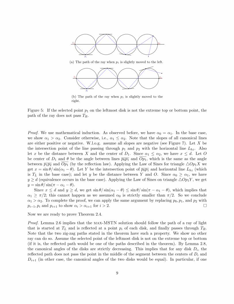
(a) The path of the ray when p1 is slightly moved to the left.
(b) The path of the ray when p1 is slightly moved to theright.
Figure 5: If the selected point p1 on the leftmost disk is not the extreme top or bottom point, thepath of the ray does not pass TR.
Proof. We use mathematical induction. As observed before, we have α0 = α1. In the base case,we show α1 > α2. Consider otherwise, i.e., α1 ≤ α2. Note that the slopes of all canonical linesare either positive or negative. W.l.o.g. assume all slopes are negative (see Figure 7). Let X bethe intersection point of the line passing through p1 and p2 with the horizontal line Lhz. Alsolet x be the distance between X and the center of D1. Since α1 ≤ α2, we have x ≤ d. Let Obe center of D1 and θ be the angle between lines p0p1 and Op1, which is the same as the anglebetween p1p2 and Op1 (by the reflection law). Applying the Law of Sines for triangle △Op1X weget x = sin θ/ sin(α1 − θ). Let Y be the intersection point of p0p1 and horizontal line Lhz (whichis TL in the base case); and let y be the distance between Y and O. Since α0 ≥ α1, we havey ≥ d (equivalence occurs in the base case). Applying the Law of Sines on triangle △Op1Y , we gety = sin θ/ sin(π − α1 − θ).
Since x ≤ d and y ≥ d, we get sin θ/ sin(α1 − θ) ≤ sin θ/ sin(π − α1 − θ), which implies thatα1 ≥ π/2; this cannot happen as we assumed α0 is strictly smaller than π/2. So we concludeα1 > α2. To complete the proof, we can apply the same argument by replacing p0, p1, and p2 withpi−1, pi and pi+1 to show αi > αi+1 for i > 2.
Now we are ready to prove Theorem 2.4.
Proof. Lemma 2.6 implies that the max-MSTN solution should follow the path of a ray of lightthat is started at TL and is reflected at a point pi of each disk, and finally passes through TR.Note that the two zig-zag paths stated in the theorem have such a property. We show no otherray can do so. Assume the selected point of the leftmost disk is not on the extreme top or bottom(if it is, the reflected path would be one of the paths described in the theorem). By Lemma 2.8,the canonical angles of the disks are strictly decreasing. This implies that for any disk Di, thereflected path does not pass the point in the middle of the segment between the centers of Di andDi+1 (in other case, the canonical angles of the two disks would be equal). In particular, if one
9
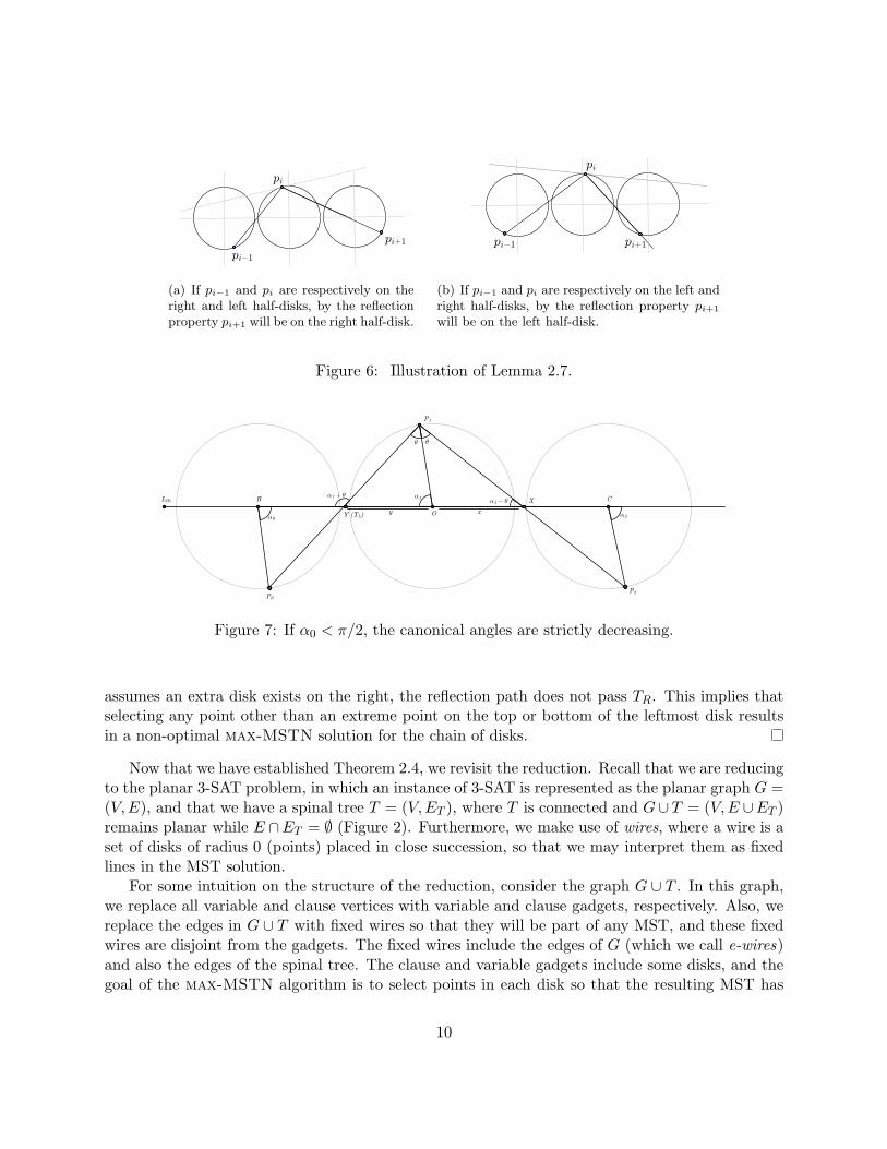
(a) If pi−1 and pi are respectively on theright and left half-disks, by the reflectionproperty pi+1 will be on the right half-disk.
(b) If pi−1 and pi are respectively on the left andright half-disks, by the reflection property pi+1
will be on the left half-disk.
Figure 6: Illustration of Lemma 2.7.
Figure 7: If α0 < π/2, the canonical angles are strictly decreasing.
assumes an extra disk exists on the right, the reflection path does not pass TR. This implies thatselecting any point other than an extreme point on the top or bottom of the leftmost disk resultsin a non-optimal max-MSTN solution for the chain of disks.
Now that we have established Theorem 2.4, we revisit the reduction. Recall that we are reducingto the planar 3-SAT problem, in which an instance of 3-SAT is represented as the planar graph G =(V,E), and that we have a spinal tree T = (V,ET ), where T is connected and G∪ T = (V,E ∪ET )remains planar while E ∩ET = ∅ (Figure 2). Furthermore, we make use of wires, where a wire is aset of disks of radius 0 (points) placed in close succession, so that we may interpret them as fixedlines in the MST solution.
For some intuition on the structure of the reduction, consider the graph G ∪ T . In this graph,we replace all variable and clause vertices with variable and clause gadgets, respectively. Also, wereplace the edges in G ∪ T with fixed wires so that they will be part of any MST, and these fixedwires are disjoint from the gadgets. The fixed wires include the edges of G (which we call e-wires)and also the edges of the spinal tree. The clause and variable gadgets include some disks, and thegoal of the max-MSTN algorithm is to select points in each disk so that the resulting MST has
10
maximum weight. Note that any MST is composed of the disconnected fixed wires that are eachconnected to some gadgets. We design the gadgets so that the e-wires (i.e., the edges of G) attachexclusively to clause gadgets. The combinatorial structure of the resulting MST includes the spinaltree as a sub-tree (that is why we call it ’spinal’); hence, an optimal max-MSTN algorithm selectsthe points in gadgets in a way to impose the maximum weight for the edges that connect the e-wiresto the spinal tree.
2.3.1 Variable Gadgets
For each variable xi, we build a set of 3c+2 disks Di in the configuration described in Theorem 2.4,spaced by d = 21/8 = 2.625, where c is the number of clauses containing instances of the variable.The reasons for the particular choices of distances are explained in the Reduction section below.The terminal points T i
L and T iR of the gadget are joined to the spinal tree of the construction.
Specifically, a wire joins T iR to T i+1
L , i ∈ {1, . . . , n− 1} for each of the n variable gadgets. Assumefor ease of discussion that the centers of Di are incident upon a horizontal line Lhz, so that theterms above, below, left, and right are well defined.
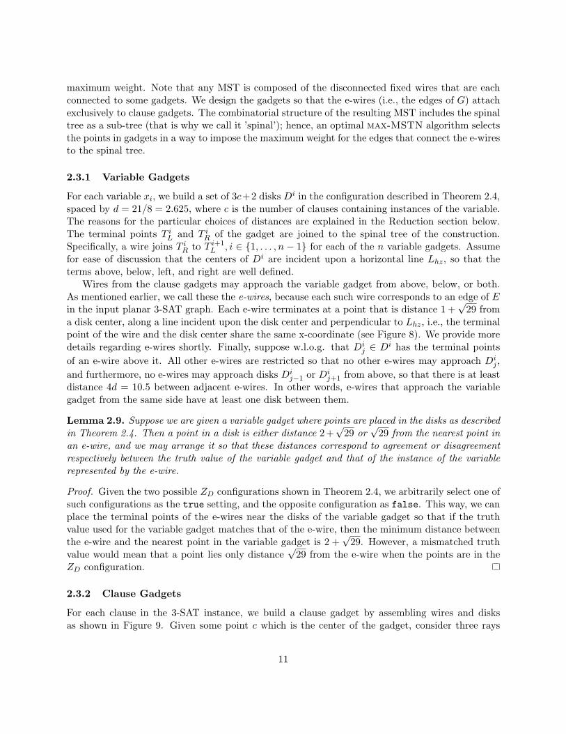
Wires from the clause gadgets may approach the variable gadget from above, below, or both.As mentioned earlier, we call these the e-wires, because each such wire corresponds to an edge of Ein the input planar 3-SAT graph. Each e-wire terminates at a point that is distance 1 +
√29 from
a disk center, along a line incident upon the disk center and perpendicular to Lhz, i.e., the terminalpoint of the wire and the disk center share the same x-coordinate (see Figure 8). We provide moredetails regarding e-wires shortly. Finally, suppose w.l.o.g. that Di
j ∈ Di has the terminal points
of an e-wire above it. All other e-wires are restricted so that no other e-wires may approach Dij ,
and furthermore, no e-wires may approach disks Dij−1 or Di
j+1 from above, so that there is at leastdistance 4d = 10.5 between adjacent e-wires. In other words, e-wires that approach the variablegadget from the same side have at least one disk between them.
Lemma 2.9. Suppose we are given a variable gadget where points are placed in the disks as describedin Theorem 2.4. Then a point in a disk is either distance 2+
√29 or
√29 from the nearest point in
an e-wire, and we may arrange it so that these distances correspond to agreement or disagreementrespectively between the truth value of the variable gadget and that of the instance of the variablerepresented by the e-wire.
Proof. Given the two possible ZD configurations shown in Theorem 2.4, we arbitrarily select one ofsuch configurations as the true setting, and the opposite configuration as false. This way, we canplace the terminal points of the e-wires near the disks of the variable gadget so that if the truthvalue used for the variable gadget matches that of the e-wire, then the minimum distance betweenthe e-wire and the nearest point in the variable gadget is 2 +
√29. However, a mismatched truth
value would mean that a point lies only distance√29 from the e-wire when the points are in the
ZD configuration.
2.3.2 Clause Gadgets
For each clause in the 3-SAT instance, we build a clause gadget by assembling wires and disksas shown in Figure 9. Given some point c which is the center of the gadget, consider three rays
11
e-wire to clause gadget e-wire to clause gadget
2 +√29 ≈ 7.39
√29 ≈ 5.39
5.25
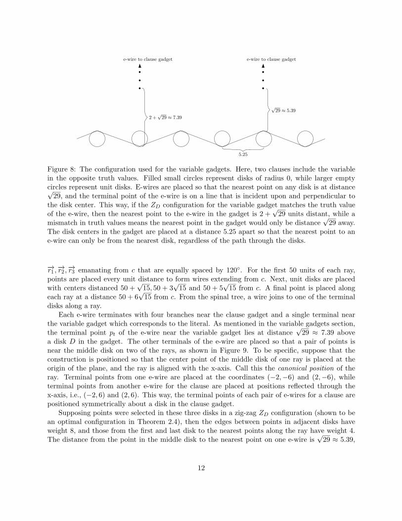
Figure 8: The configuration used for the variable gadgets. Here, two clauses include the variablein the opposite truth values. Filled small circles represent disks of radius 0, while larger emptycircles represent unit disks. E-wires are placed so that the nearest point on any disk is at distance√29, and the terminal point of the e-wire is on a line that is incident upon and perpendicular to
the disk center. This way, if the ZD configuration for the variable gadget matches the truth valueof the e-wire, then the nearest point to the e-wire in the gadget is 2 +
√29 units distant, while a
mismatch in truth values means the nearest point in the gadget would only be distance√29 away.
The disk centers in the gadget are placed at a distance 5.25 apart so that the nearest point to ane-wire can only be from the nearest disk, regardless of the path through the disks.
−→r1 ,−→r2 ,−→r3 emanating from c that are equally spaced by 120◦. For the first 50 units of each ray,points are placed every unit distance to form wires extending from c. Next, unit disks are placedwith centers distanced 50 +
√15, 50 + 3
√15 and 50 + 5
√15 from c. A final point is placed along
each ray at a distance 50 + 6√15 from c. From the spinal tree, a wire joins to one of the terminal
disks along a ray.Each e-wire terminates with four branches near the clause gadget and a single terminal near
the variable gadget which corresponds to the literal. As mentioned in the variable gadgets section,the terminal point pt of the e-wire near the variable gadget lies at distance
√29 ≈ 7.39 above
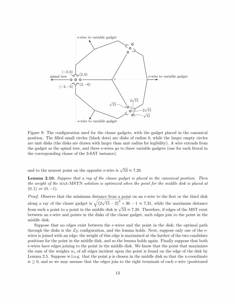
a disk D in the gadget. The other terminals of the e-wire are placed so that a pair of points isnear the middle disk on two of the rays, as shown in Figure 9. To be specific, suppose that theconstruction is positioned so that the center point of the middle disk of one ray is placed at theorigin of the plane, and the ray is aligned with the x-axis. Call this the canonical position of theray. Terminal points from one e-wire are placed at the coordinates (−2,−6) and (2,−6), whileterminal points from another e-wire for the clause are placed at positions reflected through thex-axis, i.e., (−2, 6) and (2, 6). This way, the terminal points of each pair of e-wires for a clause arepositioned symmetrically about a disk in the clause gadget.
Supposing points were selected in these three disks in a zig-zag ZD configuration (shown to bean optimal configuration in Theorem 2.4), then the edges between points in adjacent disks haveweight 8, and those from the first and last disk to the nearest points along the ray have weight 4.The distance from the point in the middle disk to the nearest point on one e-wire is
√29 ≈ 5.39,
12
cspinal tree
e-wire to variable gadget
e-wire to variable gadget
e-wire to variable gadget
2√
15
2√
15√
15
√
15
(2, 6)
(2,−6)(−2,−6)
(−2, 6)
Figure 9: The configuration used for the clause gadgets, with the gadget placed in the canonicalposition. The filled small circles (black dots) are disks of radius 0, while the larger empty circlesare unit disks (the disks are drawn with larger than unit radius for legibility). A wire extends fromthe gadget as the spinal tree, and three e-wires go to three variable gadgets (one for each literal inthe corresponding clause of the 3-SAT instance).
and to the nearest point on the opposite e-wire is√53 ≈ 7.28.
Lemma 2.10. Suppose that a ray of the clause gadget is placed in the canonical position. Thenthe weight of the max-MSTN solution is optimized when the point for the middle disk is placed at(0, 1) or (0,−1).
Proof. Observe that the minimum distance from a point on an e-wire to the first or the third disk
along a ray of the clause gadget is
√(2√15− 2
)2+ 36 − 1 ≈ 7.31, while the maximum distance
from such a point to a point in the middle disk is√53 ≈ 7.28. Therefore, if edges of the MST exist
between an e-wire and points in the disks of the clause gadget, such edges join to the point in themiddle disk.
Suppose that no edges exist between the e-wires and the point in the disk; the optimal paththrough the disks is the ZD configuration, and the lemma holds. Next, suppose only one of the e-wires is joined with an edge; the weight of this edge is maximized at the farther of the two candidatepositions for the point in the middle disk, and so the lemma holds again. Finally suppose that bothe-wires have edges joining to the point in the middle disk. We know that the point that maximizesthe sum of the weights ws of all edges incident upon the point is found on the edge of the disk byLemma 2.5. Suppose w.l.o.g. that the point p is chosen in the middle disk so that the x-coordinateis ≥ 0, and so we may assume that the edges join to the right terminals of each e-wire (positioned
13
at (2, 6) and (2,−6)). The distance from these two points to a point on the right half of a unitcircle centered at the origin is maximized at either (0, 1) or (0,−1), and so the lemma follows.
Lemma 2.11. If all three e-wires associated with a clause gadget are joined to the clause gadgetswith edges, then the weight of these edges is maximized when two e-wires are joined with edges ofweight
√29, and the other is joined with an edge of weight
√53.
Proof. By Lemma 2.10, we know that all clause gadgets will use the ZD configuration through theirdisks. Therefore, the weight of an edge between the clause gadget and an e-wire is either
√29 or√
53. Further, because two e-wires approach each set of disks, if one e-wire is distance√29 from a
point in the clause, then another e-wire is√53 from the same point. The e-wires are arranged so
that each pair of e-wires associated with a clause gadget has this relationship. Therefore, there aretwo possible settings:
1. Each e-wire is distance√29 from the nearest point in the clause gadget.
2. One e-wire is distance√53 from the nearest point in the clause gadget, while the other two
e-wires are distance√29 from the nearest point in the clause gadget. The configuration of
the path through the triple of disks between the latter two e-wires is inconsequential.
Since we are computing a minimum spanning tree with maximum weight, the second configurationis preferable.
2.3.3 Reduction
The key to the reduction is that if and only if there exists a satisfying assignment to a given planar3-SAT instance, then an optimal max-MSTN solution to the construction outlined above will joinall of the e-wires to the clause gadgets, leaving the variable gadgets unaffected. Therefore, we beginthe reduction by determining the weight of an optimal solution. If there is no satisfying assignment,the optimal max-MSTN algorithm selects the points in a way that the ZD path through at leastone variable gadget is affected, and the total weight of the optimal max-MSTN solution is reduced.We determine a lower bound on this effect, and in so doing, establish the hardness of the problem.
Let us consider the structure of an optimal solution to max-MSTN if there exists a satisfyingassignment, and in particular we examine the weights of the edges required to join each of thethree e-wires associated with a clause gadget (the same reasoning applies to all clause gadgets).Recall that an e-wire may be distance
√29 ≈ 5.39 or
√53 ≈ 7.28 from the nearest point in
the clause gadget, by Lemma 2.10. Assuming that the points in the variable gadget are in theZD configuration, the nearest point to an e-wire in the variable gadget may be
√29 ≈ 5.39 or√
29+ 2 ≈ 7.39, by Lemma 2.9. Since at least one of the literals may be satisfied in the clause, thecorresponding e-wire, call it esat, is distance 7.39 from its variable gadget when the variable gadgethas the ZD configuration associated with the satisfying truth assignment. To maximize the weightof the max-MSTN solution, the paths through the disks in the clause gadget should be set so thatesat is
√53 from the nearest point in each of the two disks that it approaches. Thus, the weight
of the edge to connect to esat is√53. The other two e-wires, whether they correspond to literals
that may be satisfied or not, are each connected with an edge of weight√29, by Lemma 2.11.
Since no point in any variable gadget is closer to an e-wire than the points in the clause gadget, we
14
have shown that the e-wires are all joined to the clause gadget in an optimal max-MSTN solution.Therefore, all variable gadgets are connected to the rest of the MST only at their endpoints and,by Theorem 2.4, selecting a setting other than the ZD configuration in any variable gadget issub-optimal.
We now compute the optimal weight of a max-MSTN solution under the assumption thatthere exists a satisfying assignment to the planar 3-SAT instance. Let wst be the total weight ofthe MST over the wires in the spinal tree segments of the construction, and let wew be that forthe e-wires, which are both fixed for any max-MSTN solution. The max-MSTN solution over theclause gadgets has weight 3(50+24)+2
√29+
√53 ≈ 240.05, i.e., 50 for each set of points along each
of the three rays before the disks, 24 is the weight of the optimal ZD path through the disks, andtwo e-wires are connected with edges of weight
√29 while the remaining one is connected with one
of weight√53. Therefore, given that there are m clauses, the total weight for all clause gadgets is
wcg = m(3(50+ 24)+ 2√29+
√53). Finally, assume there is a total of h disks in all of the variable
gadgets of the construction. The total weight of the optimal ZD configuration in these disks iswvg = h
√5.252 + 22 ≈ h · 5.62. Therefore, the total weight of the optimal max-MSTN solution is
wtot = wst +wew +wcg +wvg, all of which we can compute a priori once the max-MSTN instanceis constructed.
Now consider the case that there is no satisfying assignment for the 3-SAT instance. Considera truth assignment (defined by the alignment of zig-zag paths in variable gadgets) and a clausethat is not satisfied by that assignment (such a clause exists since the 3-SAT instance is notsatisfiable). Note that a max-MSTN algorithm might deviate from selecting zig-zag paths; thiswill be addressed shortly. For the clause that is not satisfied, we may dismiss the setting whereeach e-wire is
√29 from a point in the clause gadget as sub-optimal, by Lemma 2.11. Therefore,
one of the e-wires, call it ensat, is√53 from the nearest point in the clause gadget, and this affects
the positions of the points in the corresponding variable gadget at the other end of the e-wire2.Let pvg be the nearest point in the variable gadget to ensat. Notice that the Fermat point of thetwo points neighboring pvg in the variable gadget and the nearest point in ensat lies above the diskcontaining pvg, so moving pvg down within the disk increases the weight of the total MST if thereis an edge between pvg and the nearest point in ensat. Moving the point at least
√53 away from
ensat increases the weight of the max-MSTN solution as much as possible. Now the configurationof the clause gadget is the same as in the satisfying assignment above, so we need only measurethe reduction in weight resulting from the changes to the points in the variable gadget to see thetotal reduction in weight relative to an optimal max-MSTN solution for a satisfying assignment.
To determine a lower bound on this effect, assume that there is only one transition in the zig-zag pattern. That is, assume w.l.o.g. that at some point that the ZD configuration is in the true
setting, and then the pattern switches to the false setting for the remainder of the gadget. Allthe wires in the construction must maintain a minimum separation of at least
√53 to preserve the
desired structure of the MST, and so e-wires that approach the variable gadget from the same sidemust have at least two disks between them (since they correspond to mismatched truth values),and those approaching from opposite sides may have only one disk between them. To find anappropriate bound, first we assume that the closest points to each e-wire, call these pℓ and pr,
2If the ZD configuration were maintained, then the e-wire could be joined sub-optimally to the variable gadgetwith weight
√29, since the assignment is not satisfying. However, a larger MST can be achieved by deviating from
the ZD configuration in the variable gadget.
15
remain in the positions that would be optimal for a ZD configuration, i.e., at the furthest pointpossible from the axis of the variable gadget, and then we compute the maximum weight pathbetween pℓ and pr in the gadget. Next, we bound the possible error introduced by placing pℓ andpr in the extreme positions.
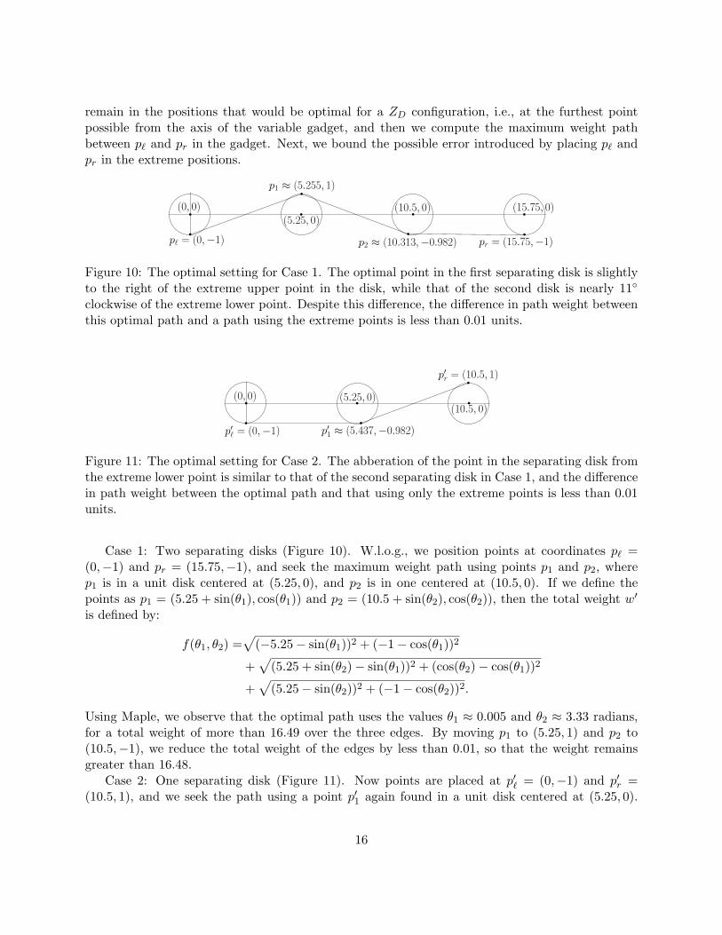
p` = (0,−1) pr = (15.75,−1)
p1 ≈ (5.255, 1)
p2 ≈ (10.313,−0.982)
(0, 0)(5.25, 0)
(10.5, 0) (15.75, 0)
Figure 10: The optimal setting for Case 1. The optimal point in the first separating disk is slightlyto the right of the extreme upper point in the disk, while that of the second disk is nearly 11◦
clockwise of the extreme lower point. Despite this difference, the difference in path weight betweenthis optimal path and a path using the extreme points is less than 0.01 units.
p′` = (0,−1)
p′r = (10.5, 1)
p′1≈ (5.437,−0.982)
(0, 0) (5.25, 0)(10.5, 0)
Figure 11: The optimal setting for Case 2. The abberation of the point in the separating disk fromthe extreme lower point is similar to that of the second separating disk in Case 1, and the differencein path weight between the optimal path and that using only the extreme points is less than 0.01units.
Case 1: Two separating disks (Figure 10). W.l.o.g., we position points at coordinates pℓ =(0,−1) and pr = (15.75,−1), and seek the maximum weight path using points p1 and p2, wherep1 is in a unit disk centered at (5.25, 0), and p2 is in one centered at (10.5, 0). If we define thepoints as p1 = (5.25 + sin(θ1), cos(θ1)) and p2 = (10.5 + sin(θ2), cos(θ2)), then the total weight w′
is defined by:
f(θ1, θ2) =√
(−5.25− sin(θ1))2 + (−1− cos(θ1))2
+√
(5.25 + sin(θ2)− sin(θ1))2 + (cos(θ2)− cos(θ1))2
+√
(5.25− sin(θ2))2 + (−1− cos(θ2))2.
Using Maple, we observe that the optimal path uses the values θ1 ≈ 0.005 and θ2 ≈ 3.33 radians,for a total weight of more than 16.49 over the three edges. By moving p1 to (5.25, 1) and p2 to(10.5,−1), we reduce the total weight of the edges by less than 0.01, so that the weight remainsgreater than 16.48.
Case 2: One separating disk (Figure 11). Now points are placed at p′ℓ = (0,−1) and p′r =(10.5, 1), and we seek the path using a point p′1 again found in a unit disk centered at (5.25, 0).
16
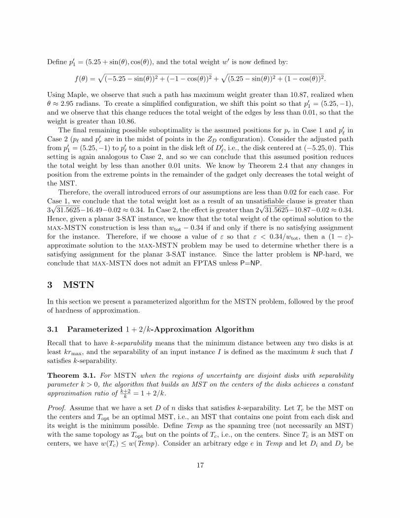
Define p′1 = (5.25 + sin(θ), cos(θ)), and the total weight w′ is now defined by:
f(θ) =√
(−5.25− sin(θ))2 + (−1− cos(θ))2 +√
(5.25− sin(θ))2 + (1− cos(θ))2.
Using Maple, we observe that such a path has maximum weight greater than 10.87, realized whenθ ≈ 2.95 radians. To create a simplified configuration, we shift this point so that p′1 = (5.25,−1),and we observe that this change reduces the total weight of the edges by less than 0.01, so that theweight is greater than 10.86.
The final remaining possible suboptimality is the assumed positions for pr in Case 1 and p′ℓ inCase 2 (pℓ and p′r are in the midst of points in the ZD configuration). Consider the adjusted pathfrom p′1 = (5.25,−1) to p′ℓ to a point in the disk left of D′
ℓ, i.e., the disk centered at (−5.25, 0). Thissetting is again analogous to Case 2, and so we can conclude that this assumed position reducesthe total weight by less than another 0.01 units. We know by Theorem 2.4 that any changes inposition from the extreme points in the remainder of the gadget only decreases the total weight ofthe MST.
Therefore, the overall introduced errors of our assumptions are less than 0.02 for each case. ForCase 1, we conclude that the total weight lost as a result of an unsatisfiable clause is greater than3√31.5625−16.49−0.02 ≈ 0.34. In Case 2, the effect is greater than 2
√31.5625−10.87−0.02 ≈ 0.34.
Hence, given a planar 3-SAT instance, we know that the total weight of the optimal solution to themax-MSTN construction is less than wtot − 0.34 if and only if there is no satisfying assignmentfor the instance. Therefore, if we choose a value of ε so that ε < 0.34/wtot, then a (1 − ε)-approximate solution to the max-MSTN problem may be used to determine whether there is asatisfying assignment for the planar 3-SAT instance. Since the latter problem is NP-hard, weconclude that max-MSTN does not admit an FPTAS unless P=NP.
3 MSTN
In this section we present a parameterized algorithm for the MSTN problem, followed by the proofof hardness of approximation.
3.1 Parameterized 1 + 2/k-Approximation Algorithm
Recall that to have k-separability means that the minimum distance between any two disks is atleast krmax, and the separability of an input instance I is defined as the maximum k such that Isatisfies k-separability.
Theorem 3.1. For MSTN when the regions of uncertainty are disjoint disks with separabilityparameter k > 0, the algorithm that builds an MST on the centers of the disks achieves a constantapproximation ratio of k+2
k = 1 + 2/k.
Proof. Assume that we have a set D of n disks that satisfies k-separability. Let Tc be the MST onthe centers and Topt be an optimal MST, i.e., an MST that contains one point from each disk andits weight is the minimum possible. Define Temp as the spanning tree (not necessarily an MST)with the same topology as Topt but on the points of Tc, i.e., on the centers. Since Tc is an MST oncenters, we have w(Tc) ≤ w(Temp). Consider an arbitrary edge e in Temp and let Di and Dj be
17
the two disks that are connected by e. Let ri and rj be the radii of Di and Dj , respectively, andlet d be the distance between Di and Dj . In Topt the disks Di and Dj are connected by an edge e′
whose weight is at least d. The weight of e on the other hand is d + ri + rj . Therefore the ratiobetween the weight of an edge in Topt and its corresponding edge in Temp is at least
d
d+ ri + rj≥ krmax
krmax + ri + rj≥ krmax
krmax + rmax + rmax=
k
k + 2.
Since this holds for any edge of Temp, we get w(Tc) ≤ w(Temp) ≤ k+2k w(Topt). Therefore we get
an approximation factor of k+2k = 1 + 2/k for the algorithm.
As with the parameterized algorithm for max-MSTN, as the disks become further apart (as kgrows), the approximation factor approaches 1.
3.2 Hardness of Approximation
To prove the hardness of the MSTN problem, we present a reduction from the planar 3-SATproblem. Recall that planar 3-SAT is a variant of 3-SAT in which the graph G = (V,E) associatedwith the formula is planar.
Theorem 3.2. MSTN does not admit an FPTAS unless P=NP.
In the hardness proof of max-MSTN, we used a spinal tree in the reduction. In this section,we use the spinal path as a path P = (Vv, EP ) with a set of edges EP such that E ∩EP = ∅, whereP passes through all variable vertices in G without crossing any edge in E. As mentioned earlier,the restricted version of planar 3-SAT remains NP-hard [8]. To reduce planar 3-SAT to MSTN,we begin by finding a planar embedding of the graph associated with the SAT formula. We forcethe inclusion of the spinal path as a part of the MST using wires. We define a wire as a set ofdisks of radius 0 placed in close succession, so that we may interpret a wire as a fixed line in theMSTN solution. We replace each variable vertex of V by a variable gadget in our construction.These gadgets are composed of a set of disks and some wires, and are defined in such a way thatwe may choose the points so that the size of the MST is equal to a certain value, if and only if theSAT formula is satisfiable.
3.2.1 Variable Gadgets
A variable gadget is formed by a k-flower, where k = 4c + 6 and c is the number of clauses inthe planar 3-SAT instance that include the variable (each clause requires 4 disks, and each of theedges of the spinal path requires 3 disks). As illustrated in Figure 12, a k-flower is composed ofk disks of unit radius, centered on the vertices of a regular k-gon. Also, each disk is tangent toits two neighboring disks, and each pair of consecutive disks Di, Di+1 intersects at a single pointqi,i+1 = Di ∩Di+1, which we call a tangent point3. Moreover, there is a k-star in the middle of the
3Using this construction, pairs of disks of the k-flower trivially intersect at a single point, which simplifies ouranalysis. To achieve strict disjointedness, the disks of the k-flower may be contracted to have radius 1 − γ so thatthe tangent point is now distance γ from the nearest point in the adjacent disks. Any path which uses the tangentpoint in our analysis will have less than 2γ units of additional weight on these shrunken disks, and there are fewerthan n(4m+ 6) disks, where n and m are the number of variables and clauses respectively. Choosing an appropriatevalue of γ so that 2γn(4m+ 6) ≪ 0.845 achieves the same result as our simplified analysis.
18
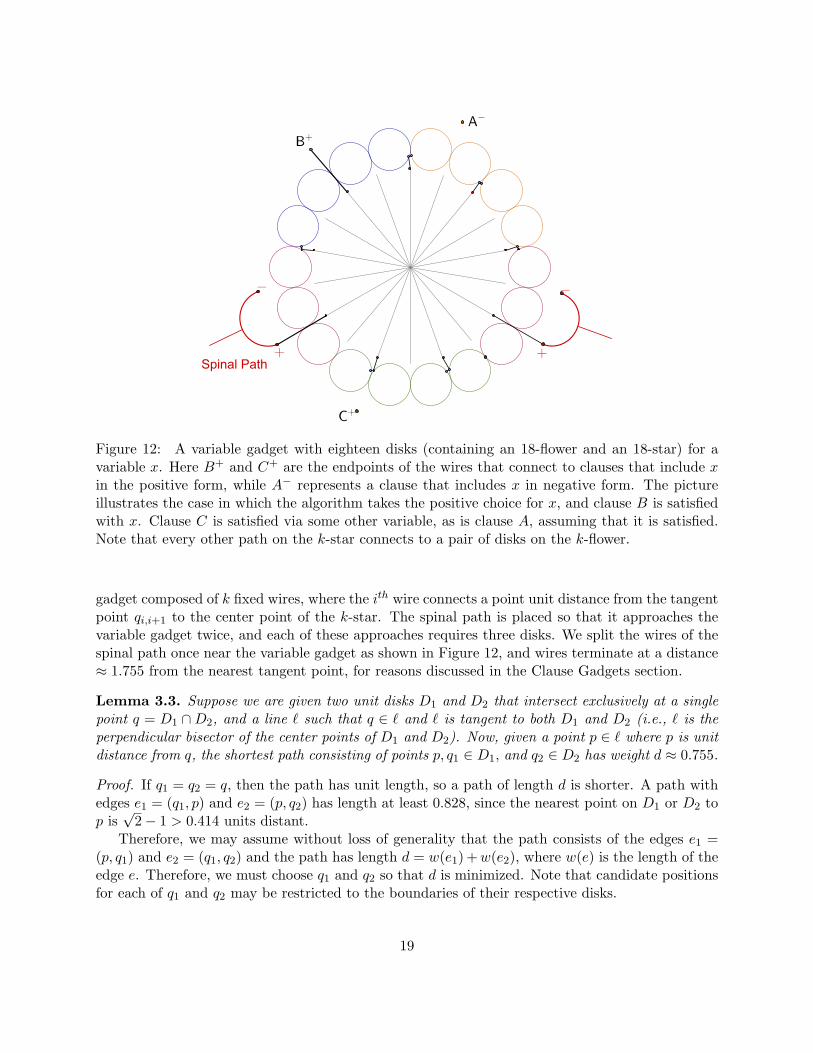
Figure 12: A variable gadget with eighteen disks (containing an 18-flower and an 18-star) for avariable x. Here B+ and C+ are the endpoints of the wires that connect to clauses that include xin the positive form, while A− represents a clause that includes x in negative form. The pictureillustrates the case in which the algorithm takes the positive choice for x, and clause B is satisfiedwith x. Clause C is satisfied via some other variable, as is clause A, assuming that it is satisfied.Note that every other path on the k-star connects to a pair of disks on the k-flower.
gadget composed of k fixed wires, where the ith wire connects a point unit distance from the tangentpoint qi,i+1 to the center point of the k-star. The spinal path is placed so that it approaches thevariable gadget twice, and each of these approaches requires three disks. We split the wires of thespinal path once near the variable gadget as shown in Figure 12, and wires terminate at a distance≈ 1.755 from the nearest tangent point, for reasons discussed in the Clause Gadgets section.
Lemma 3.3. Suppose we are given two unit disks D1 and D2 that intersect exclusively at a singlepoint q = D1 ∩D2, and a line ℓ such that q ∈ ℓ and ℓ is tangent to both D1 and D2 (i.e., ℓ is theperpendicular bisector of the center points of D1 and D2). Now, given a point p ∈ ℓ where p is unitdistance from q, the shortest path consisting of points p, q1 ∈ D1, and q2 ∈ D2 has weight d ≈ 0.755.
Proof. If q1 = q2 = q, then the path has unit length, so a path of length d is shorter. A path withedges e1 = (q1, p) and e2 = (p, q2) has length at least 0.828, since the nearest point on D1 or D2 top is
√2− 1 > 0.414 units distant.
Therefore, we may assume without loss of generality that the path consists of the edges e1 =(p, q1) and e2 = (q1, q2) and the path has length d = w(e1) +w(e2), where w(e) is the length of theedge e. Therefore, we must choose q1 and q2 so that d is minimized. Note that candidate positionsfor each of q1 and q2 may be restricted to the boundaries of their respective disks.
19
−0.1
−0.2
0
0.1
0.2
0.2 0.4 0.6 0.8 1p
q1
q2
D1
D2
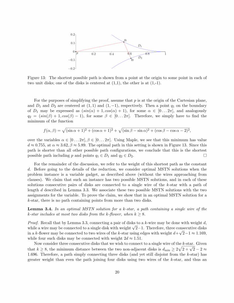
Figure 13: The shortest possible path is shown from a point at the origin to some point in each oftwo unit disks; one of the disks is centered at (1,1), the other is at (1,-1).
For the purposes of simplifying the proof, assume that p is at the origin of the Cartesian plane,and D1 and D2 are centered at (1, 1) and (1,−1), respectively. Then a point q1 on the boundaryof D1 may be expressed as (sin(α) + 1, cos(α) + 1), for some α ∈ [0 . . . 2π], and analogouslyq2 = (sin(β) + 1, cos(β) − 1), for some β ∈ [0 . . . 2π]. Therefore, we simply have to find theminimum of the function
f(α, β) =√
(sinα+ 1)2 + (cosα+ 1)2 +√
(sinβ − sinα)2 + (cosβ − cosα− 2)2,
over the variables α ∈ [0 . . . 2π], β ∈ [0 . . . 2π]. Using Maple, we see that this minimum has valued ≈ 0.755, at α ≈ 3.62, β ≈ 5.89. The optimal path in this setting is shown in Figure 13. Since thispath is shorter than all other possible path configurations, we conclude that this is the shortestpossible path including p and points q1 ∈ D1 and q2 ∈ D2.
For the remainder of the discussion, we refer to the weight of this shortest path as the constantd. Before going to the details of the reduction, we consider optimal MSTN solutions when theproblem instance is a variable gadget, as described above (without the wires approaching fromclauses). We claim that such an instance has two possible MSTN solutions, and in each of thesesolutions consecutive pairs of disks are connected to a single wire of the k-star with a path oflength d described in Lemma 3.3. We associate these two possible MSTN solutions with the twoassignments for the variable. To prove the claim, we show that in an optimal MSTN solution for ak-star, there is no path containing points from more than two disks.
Lemma 3.4. In an optimal MSTN solution for a k-star, a path containing a single wire of thek-star includes at most two disks from the k-flower, when k ≥ 8.
Proof. Recall that by Lemma 3.3, connecting a pair of disks to a k-wire may be done with weight d,while a wire may be connected to a single disk with weight
√2−1. Therefore, three consecutive disks
in a k-flower may be connected to two wires of the k-star using edges with weight d+√2−1 ≈ 1.169,
while four such disks may be connected with weight 2d ≈ 1.51.Now consider three consecutive disks that we wish to connect to a single wire of the k-star. Given
that k ≥ 8, the minimum distance between the two non-adjacent disks is dmin ≥ 2√
2 +√2− 2 ≈
1.696. Therefore, a path simply connecting three disks (and yet still disjoint from the k-star) hasgreater weight than even the path joining four disks using two wires of the k-star, and thus an
20
optimal path containing one wire of a k-star in the MST contains points from at most two disks ofthe k-flower.
Corollary 3.5. In the optimal MSTN solution for a k-flower (when k is even), each consecutivepair of disks is connected to a single wire of the k-star via a path of length d.
This follows immediately from Lemmas 3.3 and 3.4. Hence, there are two possible solutionsfor MSTN on a k-flower where k is an even number (this is the case in our construction). We usethis fact to assign a truth value for the variable gadget: one configuration is arbitrarily consideredto be true, the other false. In Figure 12, we show an example where the true configuration isused, and every other wire of the k-star has an edge to some point in the k-flower. The false
configuration would contain edges between the complementary set of wires of the k-star and thedisks of the k-flower.
3.2.2 Clause Gadgets
The clause gadgets are composed of three wires that meet at a single point. Each wire of theclause gadget is placed so that it terminates at a distance 1 + d from a tangent point, where theterminal point is collinear with a line of the k-star on the relevant variable gadget. As a result, aline segment of length 2 + d units can connect the clause gadget to the k-star of a variable gadget,while also intersecting the shared point between two disks of the k-flower. If the truth value ofthe k-flower gadget matches that of the clause, this means that connecting the clause to the flowerrequires two units of extra weight, since otherwise the two disks are connected to the k-star withd weight, as outlined in Lemma 3.3. Therefore, given a clause gadget where at least one literalmatches the truth value of the corresponding variable gadget, the clause gadget is connected to theMST with two units of additional weight.
The spinal path wires terminate in positions exactly analogous to those of the clause gadgetsso that the analysis is the same. This raises the possibility that the wires of a clause gadgetmay be connected to two variable gadgets, leaving a gap in the spinal path, but note that such aconfiguration does not affect the weight of the optimal tree. The spinal path is necessary however,since some variables may not be used by any clauses in an optimal solution.
Lemma 3.6. Joining a clause wire to a k-flower that has a truth value differing from that ofthe clause requires at least ≈ 0.845 units of additional edge weight relative to a configuration withmatching truth values.
Proof. In an optimal MSTN solution on a construction corresponding to a satisfiable 3SAT instance,a pair of disks and a clause wire may be joined to the k-star with weight 2+d units, and an additionaladjacent pair of disks may be joined to the k-star with a path of weight d. Therefore, the totalweight of the edges incident upon points in four such disks is 2 + 2d.
Now consider a configuration where the truth value of the literal for each variable in a clausedoes not match the truth value of the corresponding variable gadgets. Connecting one of the clausegadget wires to the k-star requires an additional weight of 2 + d, as discussed previously, whichintersects points from two disks; call them Di and Di+1. The neighboring two disks in the k-flower,Di−1 and Di+2, are not attached to the k-star by paths like those found in Lemma 3.3. Rather, eachof these adjacent paths may be shortened to
√2 to cover the two singleton disks. Note that there
21
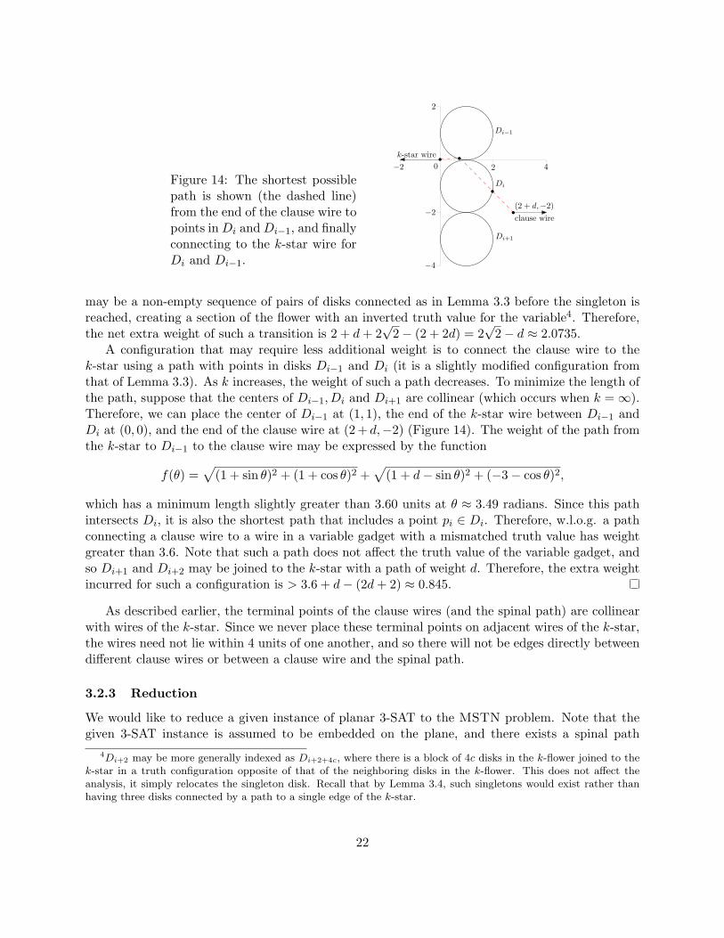
Figure 14: The shortest possiblepath is shown (the dashed line)from the end of the clause wire topoints inDi andDi−1, and finallyconnecting to the k-star wire forDi and Di−1.
Di−1
Di
Di+1
2
0−2 2 4
−2
−4
k-star wire
clause wire
(2 + d,−2)
may be a non-empty sequence of pairs of disks connected as in Lemma 3.3 before the singleton isreached, creating a section of the flower with an inverted truth value for the variable4. Therefore,the net extra weight of such a transition is 2 + d+ 2
√2− (2 + 2d) = 2
√2− d ≈ 2.0735.
A configuration that may require less additional weight is to connect the clause wire to thek-star using a path with points in disks Di−1 and Di (it is a slightly modified configuration fromthat of Lemma 3.3). As k increases, the weight of such a path decreases. To minimize the length ofthe path, suppose that the centers of Di−1, Di and Di+1 are collinear (which occurs when k = ∞).Therefore, we can place the center of Di−1 at (1, 1), the end of the k-star wire between Di−1 andDi at (0, 0), and the end of the clause wire at (2+ d,−2) (Figure 14). The weight of the path fromthe k-star to Di−1 to the clause wire may be expressed by the function
f(θ) =√
(1 + sin θ)2 + (1 + cos θ)2 +√
(1 + d− sin θ)2 + (−3− cos θ)2,
which has a minimum length slightly greater than 3.60 units at θ ≈ 3.49 radians. Since this pathintersects Di, it is also the shortest path that includes a point pi ∈ Di. Therefore, w.l.o.g. a pathconnecting a clause wire to a wire in a variable gadget with a mismatched truth value has weightgreater than 3.6. Note that such a path does not affect the truth value of the variable gadget, andso Di+1 and Di+2 may be joined to the k-star with a path of weight d. Therefore, the extra weightincurred for such a configuration is > 3.6 + d− (2d+ 2) ≈ 0.845.
As described earlier, the terminal points of the clause wires (and the spinal path) are collinearwith wires of the k-star. Since we never place these terminal points on adjacent wires of the k-star,the wires need not lie within 4 units of one another, and so there will not be edges directly betweendifferent clause wires or between a clause wire and the spinal path.
3.2.3 Reduction
We would like to reduce a given instance of planar 3-SAT to the MSTN problem. Note that thegiven 3-SAT instance is assumed to be embedded on the plane, and there exists a spinal path
4Di+2 may be more generally indexed as Di+2+4c, where there is a block of 4c disks in the k-flower joined to thek-star in a truth configuration opposite of that of the neighboring disks in the k-flower. This does not affect theanalysis, it simply relocates the singleton disk. Recall that by Lemma 3.4, such singletons would exist rather thanhaving three disks connected by a path to a single edge of the k-star.
22
P = (Vv, EP ) that passes all variable vertices without crossing any edge of G, such that all variablevertices but 2 have degree 2 in P (as mentioned at the beginning of Section 3.2, this restrictedversion is also NP-hard).
To create the instance of the MSTN problem, we fix the spinal path as a part of the MST,using wires consisting of disks of radius 0. We replace each variable node with a variable gadgetas explained. Each clause gadget includes three wires, which we place so that they approach theassociated variable gadgets as described.
The wires forming the spinal path, the m clause gadgets, and each of the n k-stars have a fixedweight, call the total weight of all these wires wwires. The remaining weight of the MST is that ofconnecting to a point from each disk in the k-flowers, and that of connecting each clause gadget.Suppose there exists a satisfying assignment for the 3-SAT instance. Each pair of disks in thek-flowers can be connected with weight d; this will be the case for all but m pairs. The remainingm pairs will be connected with edges that also join to the clause gadgets in the manner describedin Section 3.2.2 with weight 2 + d. Therefore, assuming that there is a total of i pairs of disks inthe k-flowers of the construction, the remaining weight of the MST is wdisks = id + 2m. Thus, ifthere exists a satisfying assignment to the 3-SAT instance, the total optimal weight of the MST iswtot = wwires + wdisks.
If there is no satisfying assignment, at least one of the clause gadgets must be connected to theMST in the manner described in Lemma 3.6, which requires an additional weight of at least 0.845.Now suppose there exists an FPTAS for MSTN. Given an instance of planar 3-SAT, we build theMSTN construction and determine wtot. We choose a value of ε so that ε < 0.845/wtot, and soa (1 + ε)-approximate solution to the MSTN problem may be used to determine whether thereis a satisfying assignment for the planar 3-SAT instance. Since the latter problem is NP-hard, weconclude that MSTN does not admit an FPTAS unless P=NP.
4 Conclusions
We considered geometric MST with neighborhoods problems, and established that computing theMST of minimum or maximum weight is hard to approximate in this setting by proving that thereis no FPTAS for either problem, assuming P = NP. We provided a parameterized algorithm for theMSTN problem based upon how well separated the disks are from one another. For max-MSTN,we showed that a deterministic algorithm that selects disk centers gives an approximation ratio of1/2. Furthermore, we showed that when the instance of the problem satisfies k-separability, thesame approach achieves a constant approximation ratio of 1− 2
k+4 .For further research, it will be interesting to study this problem under different models of
imprecision. Depending on the application, the regions of uncertainty may consist of other shapes,e.g., line segments, rectangles, etc., or they may be composed of discrete sets of points.
References
[1] Arkin, E., Hassin, R.: Approximation algorithms for the geometric covering salesman problem.Discrete Applied Mathematics 55(3), 197 – 218 (1994)
23
[2] de Berg, M., Gudmundsson, J., Katz, M., Levcopoulos, C., Overmars, M., van der Stappen,A.: TSP with neighborhoods of varying size. Journal of Algorithms 57(1), 22 – 36 (2005)
[3] Callahan, P.B., Kosaraju, S.R.: A decomposition of multidimensional point sets with applica-tions to k-nearest-neighbors and n-body potential fields. J. ACM 42(1), 67–90 (1995)
[4] Dumitrescu, A., Mitchell, J.S.: Approximation algorithms for TSP with neighborhoods in theplane. Journal of Algorithms 48(1), 135 – 159 (2003)
[5] Erlebach, T., Hoffmann, M., Krizanc, D., Mihalak, M., Raman, R.: Computing minimumspanning trees with uncertainty. In: Symposium on Theoretical Aspects of Computer Science.pp. 277–288 (2008)
[6] Fiala, J., Kratochvıl, J., Proskurowski, A.: Systems of distant representatives. Discrete AppliedMathematics 145(2), 306–316 (2005)
[7] Graham, R.L., Hell, P.: On the history of the minimum spanning tree problem. IEEE Annalsof the History of Computing 7(1), 43–57 (1985)
[8] Lichtenstein, D.: Planar formulae and their uses. SIAM J. on Computing 11(2), 329–344 (1982)
[9] Loffler, M., van Kreveld, M.: Largest and smallest convex hulls for imprecise points. Algorith-mica 56, 235–269 (2010)
[10] Nesetril, J., Milkova, E., Nesetrilova, H.: Otakar Boruvka on minimum spanning tree problemtranslation of both the 1926 papers, comments, history. Discrete Mathematics 233(13), 3 – 36(2001)
[11] Sekino, J.: n-ellipses and the minimum distance sum problem. The American MathematicalMonthly 106(3), pp. 193–202 (1999)
[12] Yang, Y.: On several geometric network design problems. Ph.D. thesis, State University ofNew York at Buffalo (2008)
[13] Yang, Y., Lin, M., Xu, J., Xie, Y.: Minimum spanning tree with neighborhoods. In: Algorith-mic Aspects in Information and Management, pp. 306–316 (2007)
24