Embed Size (px)
Citation preview
Digital Object Identifier (DOI) 10.1007/s00205-014-0731-3Arch. Rational Mech. Anal. 213 (2014) 447–490
On Minimizers of a Landau–de Gennes EnergyFunctional on Planar Domains
Dmitry Golovaty & José Alberto Montero
Communicated by D. Kinderlehrer
Abstract
We study tensor-valued minimizers of the Landau–de Gennes energy functionalon a simply-connected planar domainΩ with non-contractible boundary data. Herethe tensorial field represents the second moment of a local orientational distributionof rod-like molecules of a nematic liquid crystal. Under the assumption that theenergy depends on a single parameter—a dimensionless elastic constant ε > 0—we establish that, as ε → 0, the minimizers converge to a projection-valued mapthat minimizes the Dirichlet integral away from a single point inΩ . We also providea description of the limiting map.
1. Introduction
In this paper we study minimizers of the Landau–de Gennes (LdG) energyfunctional in the presence of disclinations. Under the assumptions that will bediscussed later in the introduction, the corresponding variational problem can bedescribed as follows. Let Ω ⊂ R
2 be a smooth, bounded, and simply-connecteddomain and denote by F1 the set of symmetric 3×3 matrices with trace 1. For eachu ∈ W 1,2(Ω, F1), set
Eε(u) =∫Ω
(|∇u|2
2+ W (u)
ε2
). (1)
Here ε > 0 is a small parameter and
W (u) = tr(q(u)) = 1
2tr
((u − u2
)2). (2)
A. Montero was supported by Fondecyt Grant No. 1100370.D. Golovaty was supported in part by the NSF grant DMS-1009849.
448 Dmitry Golovaty & José Alberto Montero
Observe that W (u) � 0 for any u ∈ F1 and W (u) = 0 if and only if u ∈ P, where
P = {A ∈ F1 : A2 = A}is the set of rank-one, orthogonal projection matrices.
Our results concern the minimizers uε of Eε among u ∈ W 1,2(Ω, F1) thatsatisfy u = g on ∂Ω for topologically nontrivial boundary data g correspondingto non-contractible curves in P. Our first result establishes the existence of a singlepoint a in the interior ofΩ such that the uε converge to a function u0 ∈ W 1,2
loc (Ω \{a},P) as ε → 0. More precisely, we prove the following
Theorem 1. Let g : ∂Ω → P be a non-contractible curve in P and supposethat uε ∈ W 1,2(Ω; F1) is a minimizer of Eε among functions u ∈ W 1,2(Ω; F1)
that satisfy the Dirichlet boundary condition u = g on ∂Ω. First, the minimiz-ers uε take values in the convex envelope of P; in particular they are uniformlybounded in ε. Second, there is a single point a in the interior of Ω such thatthe uε converge strongly (along a subsequence) to u0 ∈ W 1,2(Ω \ BR{a};P) inW 1,2(Ω \ BR{a}; F1) as ε → 0 for any fixed R > 0. Finally, for any open setU ⊂⊂ Ω \ {a}, u0 minimizes
∫U |∇v|2 among functions v ∈ W 1,2
loc (Ω \ {a};P)
satisfying v = u0 on ∂U.
To describe the structure of u0, let M3a (R) be the set of antisymmetric 3×3 matrices
and let [A; B] = AB − B A denote the commutator of matrices A and B. It turnsout that one can consider a vector field j (u0) with matrix entries
j (u0) =([
u0; ∂u0
∂x
],
[u0; ∂u0
∂y
]),
instead of u0 because u0 can always be recovered from j (u0) (the reason for thisreduces to the following standard fact: if A : [0, T ] → M3
a (R), then the solutionof the initial value problem
γ ′ = [γ ; A], γ (0) ∈ P,
takes values in P). In light of this observation, the following theorem gives a roughdescription of the limiting map u0 described in Theorem 1.
Theorem 2. Let u0 be as in Theorem 1. There is a function
ψ0 ∈ (W 1,2 ∩ L∞)(Ω; M3a (R))
and a constant anti-symmetric matrix Λ0 such that
j (u0) = 1
2πra(θ̂aΛ0)+ ∇⊥ψ0
in Ω. Here a ∈ Ω is as defined in Theorem 1, ra and θ̂a are the radial variableand the unit vector in an angular direction for polar coordinates centered at a
On Minimizers of a Landau–de Gennes Energy Functional on Planar Domains 449
respectively, and we interpret (θ̂aΛ0) and ∇⊥ψ0 as matrix-valued vector fieldsaccording to (9) and (8) respectively. Further, ψ0 satisfies
Δψ0 = 2
[∂ψ0
∂x; ∂ψ0
∂y
]+ 1
πra
[∇ψ0 · θ̂a;Λ0
],
inΩ , where we interpret ∇ψ0 · θ̂a according to (10), subject to boundary conditions
−∇ψ0 · ν =[
g; dg
dτ
]− θ̂a · τ
2πraΛ0,
on ∂Ω, where ν and τ are the outward unit normal and unit tangent vector to∂Ω, respectively. Finally, the function Zu0(x) := 1
2πra(Λ0 − u0Λ0 − Λ0u0) ∈
L2(Ω; M3a (R)).
Although we cannot prove it yet, we conjecture that the map ψ0 in Theorem 2is smooth. If in addition ∇ψ0(a) = 0, our results allow for renormalization ofEε(uε) along the lines of [3] via an expansion of Eε(uε) containing a leading termproportional to |ln ε| and bounded terms depending only on a and the boundarydata g.
Our problem is closely related to and motivated by the studies of equilibriumconfigurations of nematic liquid crystals—materials composed of rod-like mole-cules that flow like fluids, yet they retain a degree of molecular orientational ordersimilar to crystalline solids. There are several mathematical frameworks to studythe nematics, leading to different, but related variational models that we will discussnext.
The local orientational order can be described by specifying a director—a unitvector in a direction preferred by the molecules at a given point. The director fieldforms a basis of the Oseen–Frank theory for the uniaxial nematic liquid crystals[14]. Within this theory, one constructs an energy penalizing for spatial variations ofthe director, distinguishing between various elastic modes (splay, bend, twist) andtaking into account interactions with electromagnetic fields. Although this theoryhas generally been very successful in predicting equilibrium nematic configura-tions, it prohibits certain types of topological defects, for example, disclinations, asthe constraint that the director must have a unit length becomes too rigid. A possibleremedy was proposed by Ericksen [5] who introduced a scalar parameter intendedto describe the quality—the degree—of local molecular orientational order.
Despite the fact that the Ericksen’s theory is capable of handling line defects,it still assumes that a preferred direction is specified by the director, excludinga possibility that the nematic can be biaxial. Here a biaxial state differs from auniaxial state in that it has no rotational symmetry; instead it possesses reflectionsymmetries with respect to each of a three orthogonal axes (only two of whichneed to be specified). Biaxial configurations are conjectured to exist, for example,at the core of a nematic defect. Further, certain nematic configurations cannot evenbe orientable, that is, they cannot be described by a continuous director field [1].These deficiencies can be circumvented within the Landau–de Gennes theory thatwe will now briefly review (see also [1], [10], and [11]).
450 Dmitry Golovaty & José Alberto Montero
Suppose that orientations of rod-like molecules in a small neighborhood of apoint x ∈ Ω can be described in terms of a probability density function ψ(x,m) :Ω×S
2 → R+, that is, the probability that the molecules near x are oriented within
a subset S ∈ S2 is given by
p(x, S) =∫
Sψ(x,m) dσ.
Since the probabilities of finding the head or the tail of a nematic molecule pointingin a given direction are the same, the function ψ(x, ·) is even and the first momentof ψ(x, ·) vanishes. Consequently, if one were to seek a macroscopic theory basedon moments of ψ(x, ·), the simplest approach would be to use the second moment
u(x) =∫
S2m ⊗ mψ(x,m) dσ, (3)
where (a ⊗ b)i j = ai b j , i, j = 1, . . . , 3 is the tensor product of a and b.The following properties of u immediately follow from (3) and the fact that
ψ(x, ·) is a probability density function
(i) u(x) ∈ F1 and its eigenvalues satisfy λi ∈ [0, 1], i = 1, . . . , 3.(ii) u(x) = 1
3 I in an isotropic state when all molecular orientations in a vicinityof x are equally probable, that is,ψ(x,m) = 1
4π .Here I is the identity matrix.(iii) u(x) = m0 ⊗ m0 ∈ P in a perfect uniaxial nematic state when all molecules
near x are parallel to ±m0, that is, ψ(x,m) = 12 (δ(m − m0)+ δ(m + m0)).
For other forms of ψ(x, ·), the set of eigenvalues of u(x) differs from those in (i)and (ii) and the nematic is in intermediate states of order that can be either uniaxialwith a degree of orientation less than 1, or biaxial.
In thermotropic nematics, a phase transition from an isotropic to a nematic stateoccurs as the temperature is decreased below a certain threshold value. The best wayto account for a symmetry change during the transition is to define an appropriateorder parameter. Within the LdG phenomenological theory, the role of the orderparameter is played by the second order tensor Q equal to u defined in the previousparagraph, translated by a factor of 1
3 I . The theory is based on the hypothesis thatequilibrium properties of the system can be found from a non-equilibrium freeenergy, constructed as an O(3)-symmetric expansion in powers of Q.
In this paper we formulate our results in terms of the matrix u for the reasonsof mathematical simplicity, although they can easily be restated within a standardQ-tensor framework by incorporating the appropriate translation. We will furtherassume that the lowest energy configuration at temperatures below the isotropic-nematic transition is that of a perfect uniaxial nematic u ∈ P, while the isotropicstate u = 1
3 I minimizes the energy above the transition temperature. Since the LdGfree energy must be invariant with respect to rotations, it can only be a functionof the invariants of the matrix u. Given these conditions and incorporating theinvariants to the least possible powers, we obtain that
Wβ(u) = 2I 22 (u)− β I3(u) , (4)
On Minimizers of a Landau–de Gennes Energy Functional on Planar Domains 451
where the invariants are given by
I2(u) = 1
2
(1 − tr (u2)
), I3(u) = det(u) = 1
6
(1 − 3tr (u2)+ 2 tr
(u3)),
since the trace of u is equal 1. Simple calculations show that a perfect uniaxial stateu ∈ P is a local minimum of Wβ when 0 < β < 8 and it is a global minimumof Wβ when β � 6. The isotropic state u = 1
3 I is a local maximum of Wβ when0 < β � 4, it is a local minimum of Wβ when 4 < β < 6, and it is a globalminimum of Wβ when 6 � β � 8. Note that the expression (4) is equivalent to thestandard LdG energy for the traceless tensors, once the condition that the nematicminimum corresponds to a perfect uniaxial state is imposed. Since only two outof the three coefficients in the standard energy can be imposed independently, theadditional condition reduces the number of the coefficients to one and β aboveshould be temperature-dependent. In this work we will assume that 2 < β < 6,that is, the temperature is below that of the nematic-to-isotropic transition. Thelower bound on β will be explained later on in the text—it is related to the fact thatpredictions on the phenomenological, expansions-based LdG theory become non-physical away from the transition temperature (cf. [9]). Unless specified otherwise,for simplicity we will set β = 3, thus recovering (2).
The spatial variations of the order parameter in the LdG theory are controlled bythe term quadratic in the gradient of the order parameter. Here we will assume thatall elastic constants are equal so that this part of the energy becomes proportionalto the Dirichlet integral. Finally, we assume that the remaining (non-dimensional)elastic constant ε is small—for example, when the diameter of Ω is large—andthat the three-dimensional cylindrical domainΩ ×[−L , L] occupied by the liquidcrystal and the boundary data are such that we can ignore the dependence on theaxial spatial variable.
The Dirichlet boundary conditions on u are referred to as the strong anchoringconditions on ∂Ω in the physics literature: they impose specific preferred ori-entations on nematic molecules on surfaces bounding the liquid crystal. We areinterested in a situation in which the nematic is in a perfect uniaxial state on theboundary and has a winding number ± 1
2 ; in this case the nematic has a disclinationin Ω × [−L , L] or, equivalently, a point defect/vortex in Ω .
To summarize the discussion above, we consider a variational problem for anenergy functional Eε given in (1) that describes a nematic liquid crystal withinthe context of the Landau–de Gennes theory. The functional is defined over theset of matrix-valued functions; the principal contribution of this work is that wedo not impose any constraints on the target set F1 of 3 × 3 symmetric, trace-onematrices, beyond what is required by the LdG theory. The variational problemconsists of minimizing Eε among all u ∈ W 1,2(Ω; F1) that are subject to theDirichlet boundary condition u = g. Here Ω ⊂ R
2 is a bounded, smooth, simply-connected domain and g : ∂Ω → P represents a non-contractible curve in the setof rank-one, orthogonal projection matrices. Our main goal is to understand thebehavior of the minimizers of Eε in the limit of a vanishing elastic constant ε → 0.
Whenever possible, our approach follows the roadmap established for Ginzburg–Landau vortices by Bethuel et al. in [3]. As in that work, we find that the
452 Dmitry Golovaty & José Alberto Montero
minimizers uε of Eε have energies that blow up as |ln(ε)| when ε → 0. Theminimizers in [3] converge to an S1-valued harmonic map away from a finite set ofpoints inΩ in the limit of ε → 0.The situation is similar here, although the limitingharmonic map is P-valued and the singular set consists of a single point. On theother hand, even though the energy-estimates-based techniques from [3] can mostlybe extended to our case (albeit, nontrivially), the principal difference between thiswork and [3] is that the results in [3] that rely on the structure of harmonic maps intoS1 are no longer applicable to harmonic maps with values in P (or, equivalently, toRP
2). Inspired by Hélein’s treatment of the Bäcklund transformation [6], instead ofstudying the limiting map directly, we choose to describe it in terms of its currentvector (11). This leads us to consider solutions of the CMC equation [12] that arenot in W 1,2. The connection between the CMC equation and the LdG energy seemsto have not been made in the literature before.
In a recent work [2], Bauman et al. considered a related problem for an energyfunctional with a more general expression for the elastic energy that is definedover a more narrow admissible class of functions. The mathematical problem in [2]describes a thin nematic film with the strong orthogonal anchoring on the surfacesof the film. The anchoring forces one eigenvector of the order parameter matrixinside the film to be perpendicular to the film surface. The limiting map in [2]then takes values in RP
1 making the analysis of [2] closer to that of [3] than whatis possible for our problem. On the other hand, the additional constraint on theadmissible space of functions allows for a comparatively better description of thelimiting map.
Note that, when Ω ⊂ R3, the convergence analysis for uε is quite different
from its two-dimensional counterpart. Indeed, although the limiting map from R3
into P can also have singularities, the energies Eε(uε) of the minimizers uε areuniformly bounded as ε → 0. The interested reader can find a thorough review ofrecent work on this problem in [8].
After this work was submitted for publication, we learned that results similar toour Theorem 1 have been simultaneously obtained by Canevari [4]. However, themethods in [4] are significantly different from ours in that the author intentionallyavoids using the matrix algebra of the problem, whereas we use it extensively.
The manuscript is organized as follows: in the next section we set our nota-tion and collect some well known-facts needed for subsequent developments. InSection 3 we prove Theorem 1. In the last section we prove Theorem 2.
2. Notation
In this section we set our notation. We will denote by M3(R) the set of 3 ×3 matrices with real entries and by M3
a (R), M3s (R), and O(3) the sets of anti-
symmetric, symmetric, and orthogonal matrices, respectively. For any pair A, B ∈M3(R), we set
〈A, B〉 = tr(AT B), |A|2 = 〈A, A〉 and [A; B] = AB − B A.
In will denote the n × n identity matrix, whereas we will write I3×3 for the identitymap from M3(R) to itself.
On Minimizers of a Landau–de Gennes Energy Functional on Planar Domains 453
For any a ∈ R2, the standard polar coordinates centered at a will be denoted by
ra , θa, with r̂a , θ̂a being the corresponding unit vectors (we will drop the subscriptwhenever there is no ambiguity).
The set of rank-one orthogonal projections in R3 will be denoted by P, that is,
P = {A ∈ M3(R) : AT = A2 = A, tr(A) = 1}.It is well known that P is diffeomorphic to the real projective space. We define
L0 = inf{l(γ ) : γ a closed, non-contractible curve in P},where l(γ ) denotes the length of the curve γ . With the usual (2 to 1) covering mapfrom S
2 to P, we can associate every closed geodesic in P with a great circle in S2,
thus L0 > 0. Further, if γ1, γ2 are two closed geodesics in P, there is an orthogonalconstant matrix R ∈ O(3) such that γ2 = Rγ1 RT .
Now let
γ0(t) = 1
2
⎛⎝I3 +
⎛⎝ cos(t) sin(t) 0
sin(t) − cos(t) 00 0 −1
⎞⎠⎞⎠ (5)
represent a closed, non-contractible geodesic in P. A direct computation shows that
A0(t) = 1
2π
[γ0(t); dγ0
dt(t)
](6)
is a constant. Since any other closed geodesic in P can be written as γ1 = Rγ0 RT ,where R ∈ O(3) is a constant orthogonal matrix,
A(t) = 1
2π
[γ (t); dγ
dt(t)
]= 1
2πR
[γ0(t); dγ0
dt(t)
]RT
is constant for any closed geodesic γ in P, and
|A|2 = |A0|2 .Consider now any matrix A ∈ M3
a (R) that can be written as A = R A0 RT , whereA0 is given by (6) and R ∈ O(3). Next, solve the system of ODEs
γ ′ = [A; γ ]with the initial condition γ (0) = Rγ0(0)RT . By a uniqueness theorem for thisODE, the solution γ = Rγ0 RT is a closed geodesic. A direct computation showsthat A = [γ ; γ ′].
The previous discussion demonstrates that there is a 1 − 1 correspondencebetween closed geodesics in P and antisymmetric matrices of the form A = R A0 RT
with R ∈ O(3). We will call such an A ∈ M3a (R) an antisymmetric representative
of a geodesic.Set now
Fλ = {A ∈ M3s (R) : tr(A) = λ}.
454 Dmitry Golovaty & José Alberto Montero
We will denote by
Σ and Π
the closed convex envelope of P in F1, and the projection from F1 ontoΣ , respec-tively.
We shall make use of the following
Definition 1. Let A, B ∈ P, A = B, be any two matrices such that 〈A, B〉 = 0.The minimal rotation R(A, B) mapping A to B is the unique matrix R ∈ O(3)such that
B = R ART
and
RC RT = C
for the unique matrix C ∈ P with C A = AC = 0 and C B = BC = 0. If A = B,we define R(A, B) = I3.
Remark 1. We emphasize that
B = R(A, B)ART (A, B)
for any two A, B ∈ P such that the angle between their images is not π2 .
We will make use of the fact that R(A, B) depends smoothly on A, B ∈ P, at leastwhen A and B are close to each other. This can be seen from the next
Lemma 1. Let A, B ∈ P be such that 〈A, B〉 = 0, then
R(A, B) = exp
(1
2ln
(I3 + 2
〈A, B〉 [A; B]2 + 2[A; B]))
, (7)
where ln denotes a local inverse of the exponential map exp : M3a (R) → O(3)
near I3.
Proof. This expression is easy to establish if we take A = γ0(α) and B = γ0(β),where γ0 is given in (5). However, any two A, B ∈ P can be written in this form insome coordinate system. This proves the lemma. ��
Let now Ω ⊂ R2. We will often deal with matrix-valued functions u : Ω →
M3(R) and matrix-valued vector fields F : Ω → (M3(R))2, F = (F1, F2). Fora matrix-valued function u, the gradient and its perpendicular are given by thematrix-valued vector fields
∇u =(∂u
∂x,∂u
∂y
), ∇⊥u =
(∂u
∂y,−∂u
∂x
), (8)
respectively. For matrix-valued vector fields, the divergence and curl
∇ · F = ∂F1
∂x+ ∂F2
∂y, ∇⊥ · F = ∂F2
∂x− ∂F1
∂y
On Minimizers of a Landau–de Gennes Energy Functional on Planar Domains 455
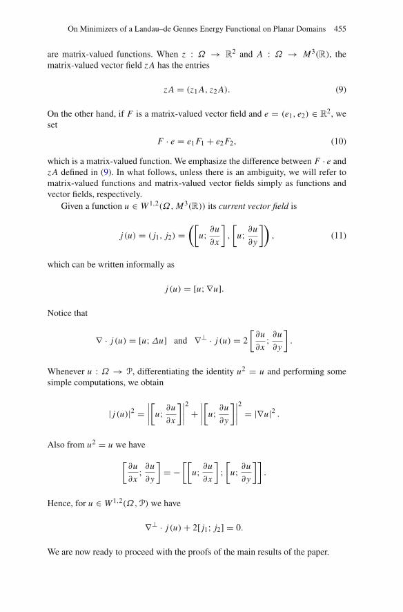
are matrix-valued functions. When z : Ω → R2 and A : Ω → M3(R), the
matrix-valued vector field z A has the entries
z A = (z1 A, z2 A). (9)
On the other hand, if F is a matrix-valued vector field and e = (e1, e2) ∈ R2, we
set
F · e = e1 F1 + e2 F2, (10)
which is a matrix-valued function. We emphasize the difference between F · e andz A defined in (9). In what follows, unless there is an ambiguity, we will refer tomatrix-valued functions and matrix-valued vector fields simply as functions andvector fields, respectively.
Given a function u ∈ W 1,2(Ω,M3(R)) its current vector field is
j (u) = ( j1, j2) =([
u; ∂u
∂x
],
[u; ∂u
∂y
]), (11)
which can be written informally as
j (u) = [u; ∇u].
Notice that
∇ · j (u) = [u;Δu] and ∇⊥ · j (u) = 2
[∂u
∂x; ∂u
∂y
].
Whenever u : Ω → P, differentiating the identity u2 = u and performing somesimple computations, we obtain
| j (u)|2 =∣∣∣∣[
u; ∂u
∂x
]∣∣∣∣2
+∣∣∣∣[
u; ∂u
∂y
]∣∣∣∣2
= |∇u|2 .
Also from u2 = u we have
[∂u
∂x; ∂u
∂y
]= −
[[u; ∂u
∂x
];[
u; ∂u
∂y
]].
Hence, for u ∈ W 1,2(Ω,P) we have
∇⊥ · j (u)+ 2[ j1; j2] = 0.
We are now ready to proceed with the proofs of the main results of the paper.
456 Dmitry Golovaty & José Alberto Montero
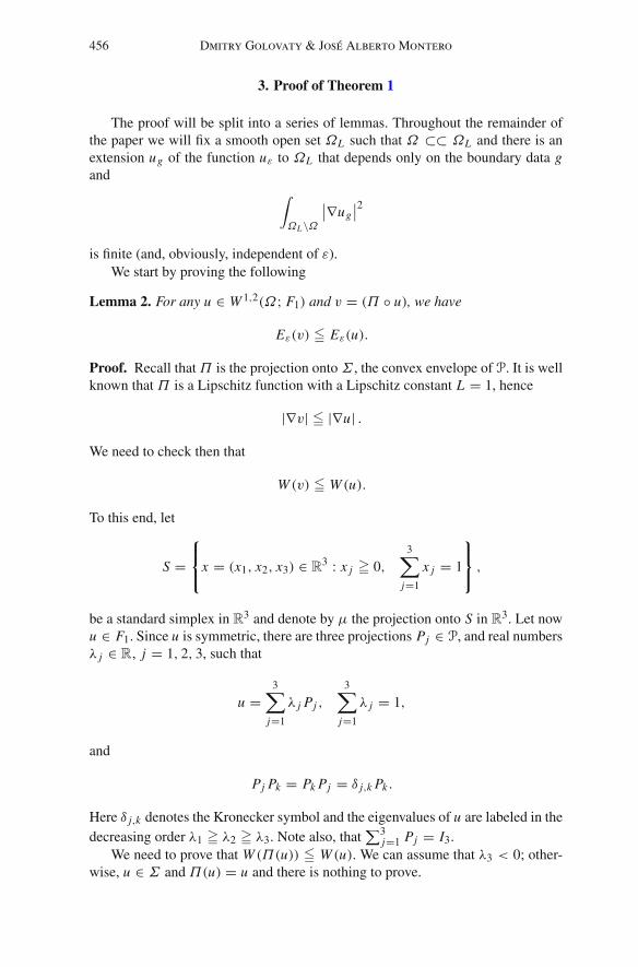
3. Proof of Theorem 1
The proof will be split into a series of lemmas. Throughout the remainder ofthe paper we will fix a smooth open set ΩL such that Ω ⊂⊂ ΩL and there is anextension ug of the function uε to ΩL that depends only on the boundary data gand
∫ΩL\Ω
∣∣∇ug∣∣2
is finite (and, obviously, independent of ε).We start by proving the following
Lemma 2. For any u ∈ W 1,2(Ω; F1) and v = (Π ◦ u), we have
Eε(v) � Eε(u).
Proof. Recall thatΠ is the projection ontoΣ , the convex envelope of P. It is wellknown that Π is a Lipschitz function with a Lipschitz constant L = 1, hence
|∇v| � |∇u| .We need to check then that
W (v) � W (u).
To this end, let
S =⎧⎨⎩x = (x1, x2, x3) ∈ R
3 : x j � 0,3∑
j=1
x j = 1
⎫⎬⎭ ,
be a standard simplex in R3 and denote by μ the projection onto S in R
3. Let nowu ∈ F1. Since u is symmetric, there are three projections Pj ∈ P, and real numbersλ j ∈ R, j = 1, 2, 3, such that
u =3∑
j=1
λ j Pj ,
3∑j=1
λ j = 1,
and
Pj Pk = Pk Pj = δ j,k Pk .
Here δ j,k denotes the Kronecker symbol and the eigenvalues of u are labeled in thedecreasing order λ1 � λ2 � λ3. Note also, that
∑3j=1 Pj = I3.
We need to prove that W (Π(u)) � W (u). We can assume that λ3 < 0; other-wise, u ∈ Σ and Π(u) = u and there is nothing to prove.
On Minimizers of a Landau–de Gennes Energy Functional on Planar Domains 457
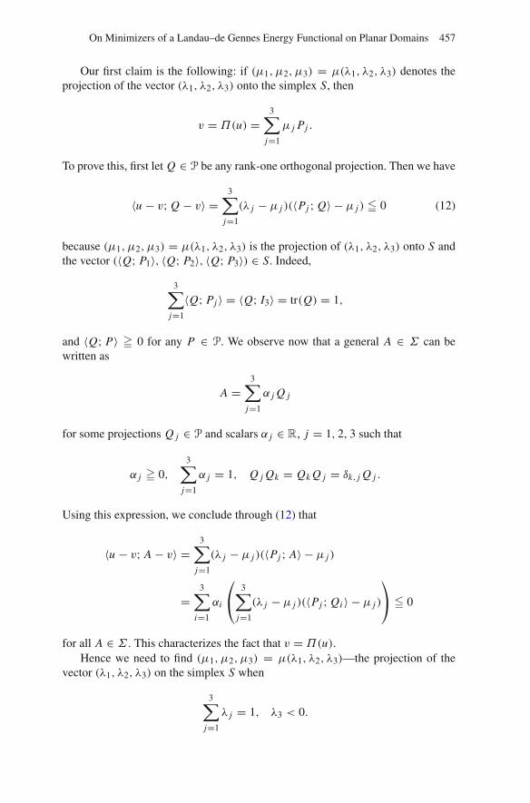
Our first claim is the following: if (μ1, μ2, μ3) = μ(λ1, λ2, λ3) denotes theprojection of the vector (λ1, λ2, λ3) onto the simplex S, then
v = Π(u) =3∑
j=1
μ j Pj .
To prove this, first let Q ∈ P be any rank-one orthogonal projection. Then we have
〈u − v; Q − v〉 =3∑
j=1
(λ j − μ j )(〈Pj ; Q〉 − μ j ) � 0 (12)
because (μ1, μ2, μ3) = μ(λ1, λ2, λ3) is the projection of (λ1, λ2, λ3) onto S andthe vector (〈Q; P1〉, 〈Q; P2〉, 〈Q; P3〉) ∈ S. Indeed,
3∑j=1
〈Q; Pj 〉 = 〈Q; I3〉 = tr(Q) = 1,
and 〈Q; P〉 � 0 for any P ∈ P. We observe now that a general A ∈ Σ can bewritten as
A =3∑
j=1
α j Q j
for some projections Q j ∈ P and scalars α j ∈ R, j = 1, 2, 3 such that
α j � 0,3∑
j=1
α j = 1, Q j Qk = Qk Q j = δk, j Q j .
Using this expression, we conclude through (12) that
〈u − v; A − v〉 =3∑
j=1
(λ j − μ j )(〈Pj ; A〉 − μ j )
=3∑
i=1
αi
⎛⎝ 3∑
j=1
(λ j − μ j )(〈Pj ; Qi 〉 − μ j )
⎞⎠ � 0
for all A ∈ Σ . This characterizes the fact that v = Π(u).Hence we need to find (μ1, μ2, μ3) = μ(λ1, λ2, λ3)—the projection of the
vector (λ1, λ2, λ3) on the simplex S when
3∑j=1
λ j = 1, λ3 < 0.
458 Dmitry Golovaty & José Alberto Montero
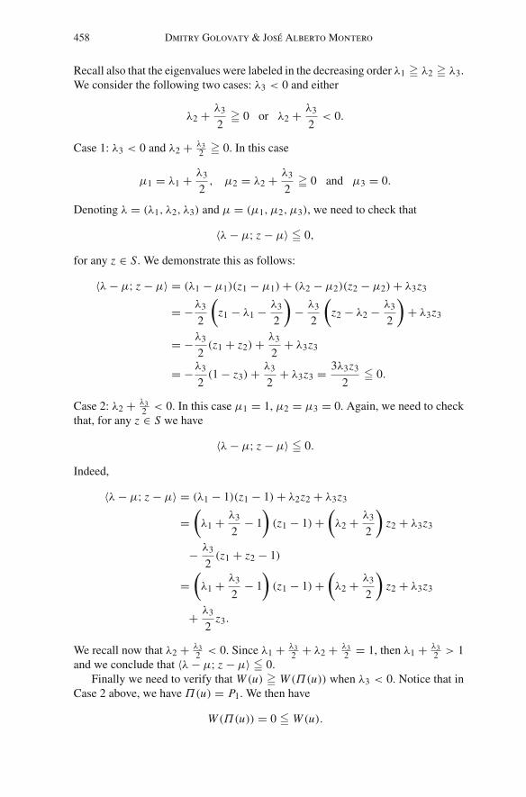
Recall also that the eigenvalues were labeled in the decreasing order λ1 � λ2 � λ3.We consider the following two cases: λ3 < 0 and either
λ2 + λ3
2� 0 or λ2 + λ3
2< 0.
Case 1: λ3 < 0 and λ2 + λ32 � 0. In this case
μ1 = λ1 + λ3
2, μ2 = λ2 + λ3
2� 0 and μ3 = 0.
Denoting λ = (λ1, λ2, λ3) and μ = (μ1, μ2, μ3), we need to check that
〈λ− μ; z − μ〉 � 0,
for any z ∈ S. We demonstrate this as follows:
〈λ− μ; z − μ〉 = (λ1 − μ1)(z1 − μ1)+ (λ2 − μ2)(z2 − μ2)+ λ3z3
= −λ3
2
(z1 − λ1 − λ3
2
)− λ3
2
(z2 − λ2 − λ3
2
)+ λ3z3
= −λ3
2(z1 + z2)+ λ3
2+ λ3z3
= −λ3
2(1 − z3)+ λ3
2+ λ3z3 = 3λ3z3
2� 0.
Case 2: λ2 + λ32 < 0. In this case μ1 = 1, μ2 = μ3 = 0. Again, we need to check
that, for any z ∈ S we have
〈λ− μ; z − μ〉 � 0.
Indeed,
〈λ− μ; z − μ〉 = (λ1 − 1)(z1 − 1)+ λ2z2 + λ3z3
=(λ1 + λ3
2− 1
)(z1 − 1)+
(λ2 + λ3
2
)z2 + λ3z3
− λ3
2(z1 + z2 − 1)
=(λ1 + λ3
2− 1
)(z1 − 1)+
(λ2 + λ3
2
)z2 + λ3z3
+ λ3
2z3.
We recall now that λ2 + λ32 < 0. Since λ1 + λ3
2 + λ2 + λ32 = 1, then λ1 + λ3
2 > 1and we conclude that 〈λ− μ; z − μ〉 � 0.
Finally we need to verify that W (u) � W (Π(u)) when λ3 < 0. Notice that inCase 2 above, we have Π(u) = P1. We then have
W (Π(u)) = 0 � W (u).
On Minimizers of a Landau–de Gennes Energy Functional on Planar Domains 459
We consider now Case 1 above. Recall that here we assumed that λ3 � λ2 � λ1,
λ3 < 0 and λ2 + λ3
2� 0.
Recall also that λ1 + λ2 + λ3 = 1. We will use the notation
s = λ1 + λ2
2, t = λ1 − λ2
2,
and observe that
s = λ1 + λ2
2= 1 − λ3
2>
1
2.
Using this notation we have that
λ1 + λ3
2= 1 + λ1 − λ2
2= 1
2+ t
and
λ2 + λ3
2= 1 + λ2 − λ1
2= 1
2− t.
Since we also have
λ1 = s + t, λ2 = s − t,
direct computations show that
W (u) = 1
2((s + t)2(s + t − 1)2 + (s − t)2(s − t − 1)2 + (2s)2(2s − 1)2).
On the other hand we have
W (Π(u)) =(
1
2+ t
)2 (1
2− t
)2
.
Denote
ψ(s, t) = 1
2((s + t)2(s + t − 1)2 + (s − t)2(s − t − 1)2 + (2s)2(2s − 1)2),
and observe that
ψ
(1
2, t
)= W (Π(u)).
To show that W (Π(u)) � W (u) it suffices to show that
∂ψ
∂s(s, t) � 0
for all s � 1/2 and all t � 0. To this end, notice first that
ψ(s, t) = q(s + t)+ q(s − t)+ q(1 − 2s) = q(s + t)+ q(s − t)+ q(2s),
460 Dmitry Golovaty & José Alberto Montero
where q(t) = t2(1−t)2
2 . Obviously
∂ψ
∂s(s, t) = q ′(s + t)+ q ′(s − t)+ 2q ′(2s).
After some algebra we arrive at
∂ψ
∂s(s, t) = 6(2s − 1)(s(3s − 1)+ t2),
which is non-negative for s � 1/2 and all t � 0. This shows that W (u) �W (Π(u)), and completes the proof of the Lemma. ��
Remark 2. The conclusion of Lemma 2 is valid for the more general form of thepotential Wβ given by (4) as long asβ � 2. We conjecture that the conclusion is falsewhen 0 < β < 2 because, in this case, a geodesic connecting two nematic minimaon the surface of Wβ expressed as a function of two independent eigenvalues of upartially lies outside of S. Since the trace of u is equal 1, at least one eigenvalue of uis negative outside of S—this violates the condition that the eigenvalues of u mustbe between 0 and 1 within the framework of the LdG theory. We conclude that ourapproach is valid for the range of the parameters corresponding to the physicallyrelevant case. The fact that the LdG theory fails in a deep nematic regime has beenpreviously discussed in [9]. The non-physicality is due to the fact that the LdG freeenergy is constructed as an expansion of the non-equilibrium free energy in termsof the order parameter near the temperature of the isotropic-to-nematic transition;the expansion no longer has to approximate the original energy away from thetransition temperature.
Remark 3. We will use Lemma 2 to establish that minimizers of Eε take values inthe convex hull of P. An alternative maximum-principle-type argument showingthat critical points of Eε with boundary data in P have values in S is given in theAppendix.
Next we collect for future reference some well-known facts regarding Q(u)—the nearest point projection of u ∈ Σ onto P. We start by choosing δ > 0 suchthat, if dist(u;P) < δ, then Q(u) is well-defined and smooth in u. Next, recall theclassical expressions
λ1(u) = sup{e · (ue) : e ∈ R3, |e| = 1},
and
λ3(u) = inf{e · (ue) : e ∈ R3, |e| = 1}.
Also, given A ∈ M3s (R), its Moore–Penrose inverse will be denoted by A†. Here
A† is the symmetric matrix that has the same kernel as A and is the inverse of A inthe subspace of R
3 where A is non-singular.
On Minimizers of a Landau–de Gennes Energy Functional on Planar Domains 461
Lemma 3. The functions λ1 and λ3 are convex and concave, respectively. Further-more, whenever u ∈ Σ is such that dist(u;P) < δ, we have
(∇uλ1)(u) = Q(u).
Finally
(Du Q)(u)(A) = (D2uλ1)(u)(A) = −(u − λ1(u)I3)
† Av − vA(u − λ1(u)I3)†.
Here we use the notation v = Q(u) and (Du Q)(u)(A) for the Jacobian matrixof Q(u) at u acting on A.
Remark 4. For v ∈ P, the expression (DvQ)(v) is the orthogonal projection fromM3
s (R) onto TvP, the tangent plane to P at v.
Proof. The fact that λ1, λ3 are convex and concave, respectively, can be obtainedvia a standard argument. Furthermore, it is well-known that
∇uλ1(u) = Q(u).
To obtain the last assertion of the lemma, let v = Q(u) and note that
(u − λ1(u)I3)v = v(u − λ1(u)I3) = 0.
Denote by ei, j := ei ⊗ e j the matrix with 1 at the (i, j)-th position and zeroseverywhere else, and differentiate the left hand side of the equation above withrespect to ui, j to obtain
0 =(
ei, j − ∂λ1
∂ui, j(u)I3
)v + (u − λ1(u)I3)
∂v
∂ui, j.
From here
(u − λ1(u)I3)∂v
∂ui, j= (u − λ1(u)I3)(I3 − v)
∂v
∂ui, j= −
(ei, j − ∂λ1
∂ui, j(u)I3
)v,
then
(I3 − v)∂v
∂ui, j= −(u − λ1(u)I3)
†(
ei, j − ∂λ1
∂ui, j(u)I3
)v = −(u − λ1(u)I3)
†ei, jv.
Taking transpose we obtain
∂v
∂ui, j(I3 − v) = −ve j,i (u − λ1(u)I3)
†.
Adding these last two equations we obtain
2∂v
∂ui, j− v
∂v
∂ui, j− ∂v
∂ui, jv = −(u − λ1(u)I3)
†ei, jv − ve j,i (u − λ1(u)I3)†.
462 Dmitry Golovaty & José Alberto Montero
We finally recall that v = Q(u) ∈ P, hence v = v2. Differentiating this expression,we obtain
v∂v
∂ui, j+ ∂v
∂ui, jv = ∂v
∂ui, j.
All this yields
∂v
∂ui, j= −(u − λ1(u)I3)
†ei, jv − ve j,i (u − λ1(u)I3)†.
Taking now A = (ai, j ) ∈ M3s (R), we multiply the above equation by ai, j and add
in i, j to obtain
(Du Q)(u)(A) = −(u − λ1(u)I3)† Av − vA(u − λ1(u)I3)
†,
which is the last conclusion of the lemma. ��Lemma 4. There is a distance r > 0, a constant C > 0, and an integer n � 2 suchthat, for any ∂Bs(a) ⊂⊂ ΩL and any u ∈ W 1,2(∂Bs(a);Σ) with dist(u;P) < ron ∂Bs(a), we have
∫∂Bs (a)
eε(u) �∫∂Bs (a)
(ρn |∇τ Q(u)|2
2+ |∇τ ρ|2
C+ 1
Cε2|1 − ρ|2
).
Here ρ = |u|, and ∇τ denotes the tangential derivative on ∂Br (a).
Proof. To prove this we write v = Q(u), and notice that, if dist(u;P) is smallenough, then
dist2(u;P) = |u − v|2 = (1 − λ1)2 + λ2
2 + λ23.
Recall that in this lemma we have u ∈ Σ , so 1 � λ1 � λ2 � λ3 � 0. In particular,if dist(u;P) < r , we have
|1 − λ1| = 1 − λ1 � dist(u;P) < r,
so λ1 > 1 − r . We also have 0 � λ2 < r . This shows that
λ1 − λ3 � λ1 − λ2 > 1 − 2r. (13)
Recall next that
∂v
∂x j= (Du Q)(u)
(∂u
∂x j
).
By the previous lemma we have
∂v
∂x j= v
∂u
∂x j(λ1(u)I3 − u)† + (λ1(u)I3 − u)†
∂u
∂x jv.
For v ∈ P and A ∈ M3s (R) we write
Tv(A) = vA(I3 − v)+ (I3 − v)Av,
On Minimizers of a Landau–de Gennes Energy Functional on Planar Domains 463
the projection of A onto TvP. Then, denoting ∇e f = e · ∇ f where e ∈ R2 is a unit
vector, we observe that
|∇eu|2 = |Tv(∇eu)|2 + |(I3×3 − Tv)(∇eu)|2 . (14)
We recall that I3×3 denotes the identity in M3(R). This last equality holds becauseTv is an orthogonal projection in M3(R). Now we have the following
∂v
∂x j= v
∂u
∂x j(λ1(u)I3 − u)† + (λ1(u)I3 − u)†
∂u
∂x jv
= Tv
(∂u
∂x j
)
+ v∂u
∂x j((λ1 I3 − u)† − (I3 − v))
+ ((λ1 I3 − u)† − (I3 − v))∂u
∂x jv.
This shows that
|∇ev|2 = |Tv(∇eu)|2
+∣∣∣v(∇eu)((λ1 I3 − u)†−(I3 − v))+((λ1 I3−u)†−(I3−v))(∇eu)v
∣∣∣2
+2〈Tv(∇eu); v(∇eu)((λ1 I3−u)†−(I3−v))〉. (15)
Let us recall now that
u = λ1v + λ2v2 + λ3v3.
for some rank-one projections v2, v3 ∈ P (with viv j = v jvi = δi, jv j , j =1, . . . , 3, v1 = v) since u ∈ Σ . Thus we have
(λ1 I3 − u)† = 1
λ1 − λ2v2 + 1
λ1 − λ3v3,
and also
(λ1 I3 − u)† − (I3 − v) =(
1
λ1 − λ2− 1
)v2 +
(1
λ1 − λ3− 1
)v3.
Notice that, for r > 0 small enough and dist(u;P) < r , this expression makessense because of (13).
Using the fact that the λ j are decreasing in j and that λ2 � 1 − λ1 we see that
λ1 − λ2 � λ1 − λ3,
and then∣∣∣(λ1 I3 − u)† − (I3 − v)
∣∣∣ � 21 − λ1 + λ2
λ1 − λ2� C(1 − λ1)
1 − 2r.
Here the constant C > 0 is independent of u and r > 0.
464 Dmitry Golovaty & José Alberto Montero
Using this expression we can now go back to (15) to obtain
|∇ev|2 � |Tv(∇eu)|2 + C(1 − λ1)
1 − 2r|∇eu|2 .
By choosing, for example 0 < r < 1/4, we get
|∇ev|2 � |Tv(∇eu)|2 + C(1 − λ1) |∇eu|2 , (16)
where C > 0 is independent of r ∈]0, 1/4].Next, we observe that
∂ |u|2∂x j
= 2 |u| ∂ |u|∂x j
= 2
⟨u; ∂u
∂x j
⟩.
In other words,
∂ |u|∂x j
=⟨
u
|u| ;∂u
∂x j
⟩.
From here we obtain
∂ |u|∂x j
=⟨
u
|u| − v; ∂u
∂x j
⟩+⟨v; ∂u
∂x j
⟩.
Since (I3×3 − Tv)(v) = v and |v| = 1, we find that
|∇e |u|| � 2|u − v|
|u| |∇eu| + |(I3×3 − Tv)(∇eu)| .
Further, due to 0 � λ3 � λ2 � 1 −λ1, we have that |u − v| � 3(1 −λ1). This and|u| � λ1 > 1 − r lead to the following inequality
|∇e |u||2 � C(1 − λ1) |∇eu|2 + C |(I3×3 − Tv)(∇eu)|2 , (17)
where C > 0 can be chosen independently of r ∈]0, 14 ]. We now use (17) and (16)
in (14) to obtain
|∇eu|2 � |∇ev| + 1
C|∇e |u||2 − C(1 − λ1) |∇eu|2 ,
or
(1 + C(1 − λ1)) |∇eu|2 � |∇ev|2 + 1
C|∇e |u||2 .
This implies that
|∇eu|2 � (1 − C(1 − λ1)) |∇ev|2 + 1
C|∇e |u||2 . (18)
Next, observe that, since the eigenvalues of u are non-negative and add up to 1, itfollows that |u| � 1 and
1 = (λ1 + λ2 + λ3)2.
On Minimizers of a Landau–de Gennes Energy Functional on Planar Domains 465
From here we find that
2(1 − |u|) � 1 − |u|2 = 1 − λ21 − λ2
2 − λ23 = 2(λ1λ2 + λ1λ3 + λ2λ3).
This implies that
(1 − |u|) � λ1(1 − λ1) � (1 − r)(1 − λ1),
so
1 − λ1 � 1 − |u|1 − r
.
Next, let n � 1 be an integer to be chosen later and write
1 − C(1 − λ1) = |u|n + (1 − |u|n)− C(1 − λ1)
= |u|n + (1 − |u|)n−1∑k=0
|u|k − C(1 − λ1)
� |u|n + (1 − |u|)(
n−1∑k=0
|u|k − C
1 − r
)
� |u|n + (1 − |u|)(
n−1∑k=0
(1 − r)k − C
1 − r
).
Now it is clear that we can choose r > 0 small enough and n � 1 large enough sothat
n−1∑k=0
(1 − r)k − C
1 − r= 1 − (1 − r)n
r− C
1 − r� 0.
With such r > 0 and n � 1 we obtain
1 − C(1 − λ1) � |u|nif dist(u;P) < r . Going back to (18), we obtain
|∇eu|2 � |u|n |∇ev|2 + 1
C|∇e |u||2 .
Finally, we observe that 2(1 − λ1) � 1 − λ21 � 0, so
8W (u) � 4λ21(1 − λ1)
2 � (1 − r)2(1 − λ21)
2
� (1 − r)2(1 − |u|2)2 � (1 − r)2(1 − |u|)2.Therefore, if r > 0 is small enough, dist(u;P) < r , and n � 1 is large enough,then
eε(u) = |∇u|22
+ W (u)
ε2
� |u|n |∇τ Q(u)|22
+ |∇τ |u||2C
+ 1
Cε2|1 − |u||2 .
The conclusion of the lemma follows since ρ = |u|. ��
466 Dmitry Golovaty & José Alberto Montero
Next we recall several lemmas that can be proven exactly as in [3].
Lemma 5. IfΩ is star-shaped, there exists a constant C > 0 independent of ε > 0such that
1
ε2
∫Ω
W (u)+∫∂Ω
|∇u · ν|2 � C.
Proof. This follows from Pohozaev’s identity, as in [3]. ��Lemma 6. Let C > 0 be such that
|∇x W (u)| � C
ε(19)
in Ω . For all 0 < r � 2C there are positive numbers λ0, μ0 > 0 such that for alll � λ0ε and all x0 ∈ Ω ,
1
ε2
∫Ω∩B2l (x0)
W (u) � μ0 ⇒ W (u(x)) � r for all x ∈ Ω ∩ Bl(x0).
Proof. Again, the proof of this statement is exactly as in [3]. We pick x0 ∈ Ω andassume that there is y0 ∈ Bl(x0) with W (u(y0)) � r . From (19) we obtain
W (u(x)) = W (u(y0))+ W (u(x))− W (u(y0))
� W (u(y0))− C
ε|x − y0|
� r − Cρ
ε,
for all x ∈ Bρ(y0). Choose ρ = εr2C . Then,
W (u(x)) � r
2
for all x ∈ Bρ(y0).Observe now that there is a number α > 0 such that |Ω ∩ Br (x)| � αr2 for
all x ∈ Ω and all 0 < r � 1. Further, y0 ∈ Bρ(x0) implies Bρ(y0) ⊂ B2l(x0),whenever l � ρ = εr
2C . We conclude that
∫Ω∩B2l (x0)
W (u) �∫Ω∩Bρ(y0)
W (u) � r
2αρ2 = αr3ε2
4C2 .
Set λ0 = r2C and 0 < μ0 <
αr3
4C2 . This proves the lemma. ��We assume now that g : ∂Ω → P represents a non-contractible curve in P.
Recall the definition of the smooth open set ΩL given in the first paragraph of thissection. In particular, we may consider uε to be defined in ΩL , but independent ofε in ΩL \Ω . Our next lemma is the following
On Minimizers of a Landau–de Gennes Energy Functional on Planar Domains 467
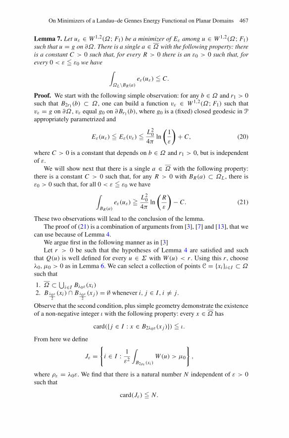
Lemma 7. Let uε ∈ W 1,2(Ω; F1) be a minimizer of Eε among u ∈ W 1,2(Ω; F1)
such that u = g on ∂Ω . There is a single a ∈ Ω with the following property: thereis a constant C > 0 such that, for every R > 0 there is an ε0 > 0 such that, forevery 0 < ε � ε0 we have ∫
ΩL\BR(a)eε(uε) � C.
Proof. We start with the following simple observation: for any b ∈ Ω and r1 > 0such that B2r1(b) ⊂ Ω , one can build a function vε ∈ W 1,2(Ω; F1) such thatvε = g on ∂Ω , vε equal g0 on ∂Br1(b), where g0 is a (fixed) closed geodesic in P
appropriately parametrized and
Eε(uε) � Eε(vε) � L20
4πln
(1
ε
)+ C, (20)
where C > 0 is a constant that depends on b ∈ Ω and r1 > 0, but is independentof ε.
We will show next that there is a single a ∈ Ω with the following property:there is a constant C > 0 such that, for any R > 0 with BR(a) ⊂ ΩL , there isε0 > 0 such that, for all 0 < ε � ε0 we have
∫BR(a)
eε(uε) � L20
4πln
(R
ε
)− C. (21)
These two observations will lead to the conclusion of the lemma.The proof of (21) is a combination of arguments from [3], [7] and [13], that we
can use because of Lemma 4.We argue first in the following manner as in [3]Let r > 0 be such that the hypotheses of Lemma 4 are satisfied and such
that Q(u) is well defined for every u ∈ Σ with W (u) < r . Using this r , chooseλ0, μ0 > 0 as in Lemma 6. We can select a collection of points C = {xi }i∈I ⊂ Ω
such that
1. Ω ⊂ ⋃i∈I Bλ0ε(xi )
2. B λ0ε2(xi ) ∩ B λ0ε
2(x j ) = ∅ whenever i, j ∈ I , i = j .
Observe that the second condition, plus simple geometry demonstrate the existenceof a non-negative integer ι with the following property: every x ∈ Ω has
card({ j ∈ I : x ∈ B2λ0ε(x j )}) � ι.
From here we define
Jε ={
i ∈ I : 1
ε2
∫B2ρε (xi )
W (u) > μ0
},
where ρε = λ0ε. We find that there is a natural number N independent of ε > 0such that
card(Jε) � N .
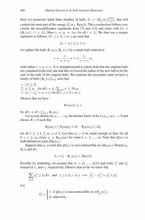
468 Dmitry Golovaty & José Alberto Montero
Next we iteratively build finite families of balls, Ci = {Brij(xi
j )}N (i)j=1 , that will
contain the main part of the energy Eε(uε; BR(a)). This construction follows veryclosely the Jerrard/Sandier arguments from [7] and [13] and starts with C0 ={Bri (xi ) : i ∈ Jε}. Here ri = ρε = λ0ε for all i ∈ Jε. We then use a mergerargument as follows: if i, j ∈ Jε, i = j are such that
∣∣xi − x j∣∣ � ri + r j ,
we replace the balls Bri (xi ), Br j (x j ) by a single ball centered at
x = ri
ri + r jxi + + r j
ri + r jx j
with radius r = ri + r j . It is straightforward to check both that the original ballsare contained in the new one and that we forced the radius of the new ball to be thesum of the radii of the original balls. We continue this procedure until we have afamily of balls {Bri (xi )}i∈J such that
1. |J | � N2. ri � ρε for all i ∈ Jε,
∑i∈J ri � Nλ0ε
3.∣∣xi − x j
∣∣ > ri + r j for all i, j ∈ J , i = j .
Observe that we have
W (u(x)) � r,
for all x ∈ Ω \ ⋃i∈J Bri (xi ).Let us now denote by a1, . . . , am the distinct limits of the {xi }i∈J as ε → 0 and
choose R > 0 such that
B2R(a j ) ∩ B2R(ak) = ∅, B2R(a j ) ⊂ ΩL
for all 1 � j, k � m, j = k. Let also ε0 > 0 be small enough so that, for all0 < ε � ε0, every x j ∈ BR/4(ak) for some k = 1, . . . ,m. Note that Q(uε) iswell-defined on each ∂BR(a j ).
Suppose that a j is such that Q(uε) is non-contractible on ∂BR(a j ). Denote a j
by a and set
J1 = { j : Br j (x j ) ⊂ BR(a)}.Possibly by relabeling, we assume that J1 = {1, . . . , k(1)} and write x1
j and ρ1j
instead of x j and r j , respectively. Observe that so far we know that
∑j∈J1
ρ1j � λ0 Nε and i, j ∈ J1, i = j �⇒
∣∣∣x1j − x1
i
∣∣∣ > ρ1j + ρ1
i .
Let
δ1j =
{1, if Q(uε) is non-contractible on ∂Bρ1
j(x1
j ),
0, otherwise.
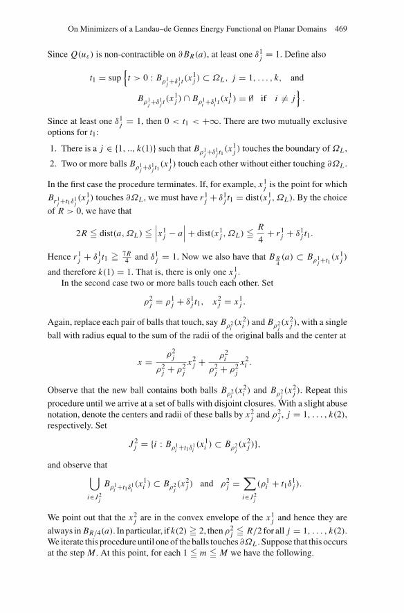
On Minimizers of a Landau–de Gennes Energy Functional on Planar Domains 469
Since Q(uε) is non-contractible on ∂BR(a), at least one δ1j = 1. Define also
t1 = sup{
t > 0 : Bρ1j +δ1
j t (x1j ) ⊂ ΩL , j = 1, . . . , k, and
Bρ1j +δ1
j t (x1j ) ∩ Bρ1
i +δ1i t (x
1i ) = ∅ if i = j
}.
Since at least one δ1j = 1, then 0 < t1 < +∞. There are two mutually exclusive
options for t1:
1. There is a j ∈ {1, .., k(1)} such that Bρ1j +δ1
j t1(x1
j ) touches the boundary ofΩL ,
2. Two or more balls Bρ1j +δ1
j t1(x1
j ) touch each other without either touching ∂ΩL .
In the first case the procedure terminates. If, for example, x1j is the point for which
Br1j +t1δ1
j(x1
j ) touches ∂ΩL , we must have r1j + δ1
j t1 = dist(x1j ,ΩL). By the choice
of R > 0, we have that
2R � dist(a,ΩL) �∣∣∣x1
j − a∣∣∣ + dist(x1
j ,ΩL) � R
4+ r1
j + δ1j t1.
Hence r1j + δ1
j t1 � 7R4 and δ1
j = 1. Now we also have that B R4(a) ⊂ Bρ1
j +t1(x1
j )
and therefore k(1) = 1. That is, there is only one x1j .
In the second case two or more balls touch each other. Set
ρ2j = ρ1
j + δ1j t1, x2
j = x1j .
Again, replace each pair of balls that touch, say Bρ2i(x2
i ) and Bρ2j(x2
j ), with a single
ball with radius equal to the sum of the radii of the original balls and the center at
x = ρ2j
ρ2j + ρ2
j
x2j + ρ2
i
ρ2j + ρ2
j
x2i .
Observe that the new ball contains both balls Bρ2i(x2
i ) and Bρ2j(x2
j ). Repeat this
procedure until we arrive at a set of balls with disjoint closures. With a slight abusenotation, denote the centers and radii of these balls by x2
j and ρ2j , j = 1, . . . , k(2),
respectively. Set
J 2j = {i : Bρ1
i +t1δ1i(x1
i ) ⊂ Bρ2j(x2
j )},and observe that⋃
i∈J 2j
Bρ1i +t1δ1
i(x1
i ) ⊂ Bρ2j(x2
j ) and ρ2j =
∑i∈J 2
j
(ρ1i + t1δ
1j ).
We point out that the x2j are in the convex envelope of the x1
j and hence they are
always in BR/4(a). In particular, if k(2) � 2, thenρ2j � R/2 for all j = 1, . . . , k(2).
We iterate this procedure until one of the balls touches ∂ΩL . Suppose that this occursat the step M . At this point, for each 1 � m � M we have the following.
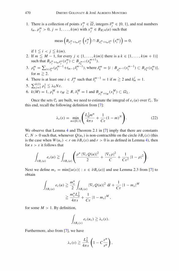
470 Dmitry Golovaty & José Alberto Montero
1. There is a collection of points xmj ∈ Ω , integers δm
j ∈ {0, 1}, and real numberstm, ρm
j > 0, j = 1, . . . , k(m) with xmj ∈ BR/4(a) such that
meas(
Bρmj +tmδm
j
(xm
j
)∩ Bρm
i +tmδmi
(xm
i
)) = 0,
if 1 � i < j � k(m).2. If m � M − 1, for every j ∈ {1, . . . , k(m)} there is a k ∈ {1, . . . , k(m + 1)}
such that Bρmj +tmδm
j(xm
j ) ⊂ Bρm+1
k(xm+1
k ).
3. ρmk = ∑
i∈J mk(ρm−1
i +tm−1δm−1i ),where J m
k = {i : Bρm−1
i(xm−1
i ) ⊂ Bρmk(xm
k )},for m � 2.
4. There is at least one i ∈ J mj such that δm−1
i = 1 if m � 2 and δ jm = 1.
5.∑k(1)
j=1 ρ11 � λ0 Nε.
6. k(M) = 1, ρM1 + tM � R, δM
1 = 1 and BρM1 +tM
(x M1 ) ⊂ ΩL .
Once the sets Ci are built, we need to estimate the integral of eε(u) over Ci . Tothis end, recall the following definition from [7]:
λε(s) = minm∈[0,1]
(L2
0mn
4πs+ 1
Cε(1 − m)N
). (22)
We observe that Lemma 4 and Theorem 2.1 in [7] imply that there are constantsC, N > 0 such that, whenever Q(uε) is non-contractible on the circle ∂Bs(x) (thisis the case when W (uε) < r on ∂Bs(x) and r > 0 is as defined in Lemma 4), thenfor s > ε it follows that
∫∂Bs (a)
eε(u) �∫∂Bs (a)
(ρn |∇τ Q(u)|2
2+ |∇τ ρ|2
C+ 1
Cε2|1 − ρ|2
).
Next we define ms = min{|u(x)| : x ∈ ∂Bs(a)} and use Lemma 2.3 from [7] toobtain
∫∂Bs (a)
eε(u) � mns
2
∫∂Bs (a)
|∇τ Q(u)|2 dl + 1
Cε|1 − ms |M
� mns L2
0
4πs+ 1
Cε|1 − ms |M ,
for some M > 1. By definition,
∫∂Bs (x)
eε(uε) � λε(s).
Furthermore, also from [7], we have
λε(s) � L20
4πs
(1 − C
εα
sα
),
On Minimizers of a Landau–de Gennes Energy Functional on Planar Domains 471
for some constants C, α > 0 that do not depend on s, ε. This shows that whenboth Q(uε) is well-defined and non-contractible and W (uε) < r in an annulusBs1 \ Bs0(x), where s0 > ε then
∫Bs1\Bs0 (x)
eε � L20
4πln
(s1
s0
)− C, (23)
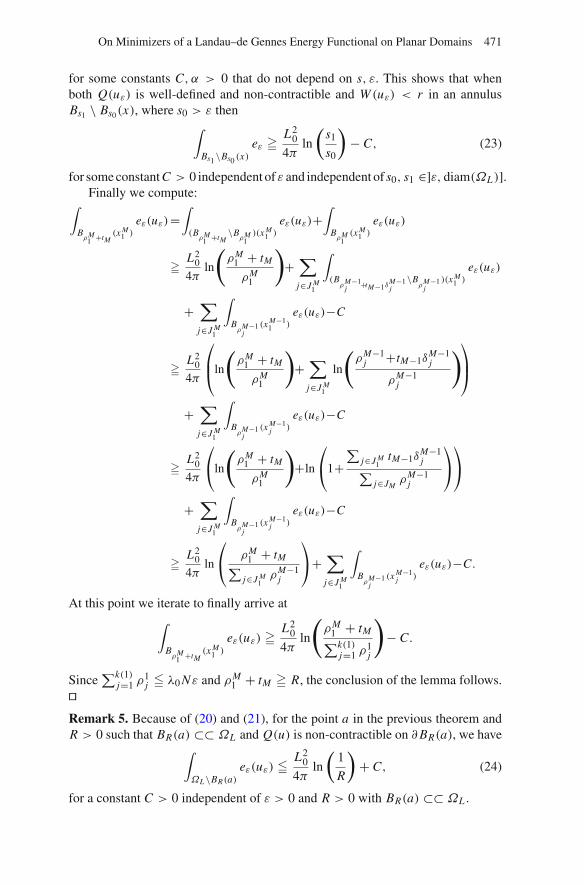
for some constant C > 0 independent of ε and independent of s0, s1 ∈]ε, diam(ΩL)].Finally we compute:∫
BρM
1 +tM(x M
1 )
eε(uε)=∫(BρM
1 +tM\B
ρM1)(x M
1 )
eε(uε)+∫
BρM
1(x M
1 )
eε(uε)
�L2
0
4πln
(ρM
1 + tM
ρM1
)+
∑j∈J M
1
∫(Bρ
M−1j +tM−1δ
M−1j
\Bρ
M−1j
)(x M1 )
eε(uε)
+∑j∈J M
1
∫Bρ
M−1j
(x M−11 )
eε(uε)−C
�L2
0
4π
⎛⎜⎝ln
(ρM
1 + tM
ρM1
)+
∑j∈J M
1
ln
(ρM−1
j +tM−1δM−1j
ρM−1j
)⎞⎟⎠
+∑j∈J M
1
∫Bρ
M−1j
(x M−1j )
eε(uε)−C
�L2
0
4π
⎛⎝ln
(ρM
1 + tM
ρM1
)+ln
⎛⎝1+
∑j∈J M
1tM−1δ
M−1j∑
j∈JMρM−1
j
⎞⎠⎞⎠
+∑j∈J M
1
∫Bρ
M−1j
(x M−1j )
eε(uε)−C
�L2
0
4πln
⎛⎝ ρM
1 + tM∑j∈J M
1ρM−1
j
⎞⎠+
∑j∈J M
1
∫Bρ
M−1j
(x M−1j )
eε(uε)−C.
At this point we iterate to finally arrive at∫
BρM
1 +tM(x M
1 )
eε(uε) � L20
4πln
(ρM
1 + tM∑k(1)j=1 ρ
1j
)− C.
Since∑k(1)
j=1 ρ1j � λ0 Nε and ρM
1 + tM � R, the conclusion of the lemma follows.��Remark 5. Because of (20) and (21), for the point a in the previous theorem andR > 0 such that BR(a) ⊂⊂ ΩL and Q(u) is non-contractible on ∂BR(a), we have∫
ΩL\BR(a)eε(uε) � L2
0
4πln
(1
R
)+ C, (24)
for a constant C > 0 independent of ε > 0 and R > 0 with BR(a) ⊂⊂ ΩL .
472 Dmitry Golovaty & José Alberto Montero
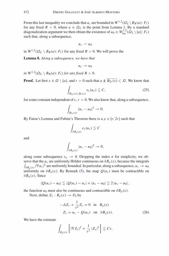
From this last inequality we conclude that uε are bounded in W 1,2(ΩL \ BR(a); F1)
for any fixed R > 0, where a ∈ ΩL is the point from Lemma 1. By a standarddiagonalization argument we then obtain the existence of u0 ∈ W 1,2
loc (ΩL \ {a}; F1)
such that, along a subsequence,
uε ⇀ u0
in W 1,2(ΩL \ BR(a); F1) for any fixed R > 0. We will prove the
Lemma 8. Along a subsequence, we have that
uε → u0
in W 1,2(ΩL \ BR(a); F1) for any fixed R > 0.
Proof. Let first x ∈ Ω \ {a}, and r > 0 such that a /∈ B2r (x) ⊂ Ω . We know that∫B2r (x)\Br (x)
eε(uε) � C, (25)
for some constant independent of ε, r > 0. We also know that, along a subsequence,∫B2r (x)
|uε − u0|2 → 0.
By Fatou’s Lemma and Fubini’s Theorem there is a ρ ∈ [r, 2r ] such that∫∂Bρ(x)
eε(uε) � C
and ∫∂Bρ(x)
|uε − u0|2 → 0,
along some subsequence εn → 0. Dropping the index n for simplicity, we ob-serve that the uε are uniformly Hölder continuous on ∂Bρ(x), because the integrals∫∂Bρ(x)
|∇uε|2 are uniformly bounded. In particular, along a subsequence, uε → u0
uniformly on ∂Bρ(x). By Remark (5), the map Q(uε) must be contractible on∂Bρ(x). Since
|Q(uε)− u0| � |Q(uε)− uε| + |uε − u0| � 2 |uε − u0| ,the function u0 must also be continuous and contractible on ∂Bρ(x).
Next, define Zε : Bρ(x) → F0 by
−ΔZε + 1
ε2 Zε = 0 in Bρ(x)
Zε = uε − Q(uε) on ∂Bρ(x). (26)
We have the estimate ∫Bρ(x)
{|∇Zε|2 + 1
ε2|Zε|2
}� Cε.
On Minimizers of a Landau–de Gennes Energy Functional on Planar Domains 473
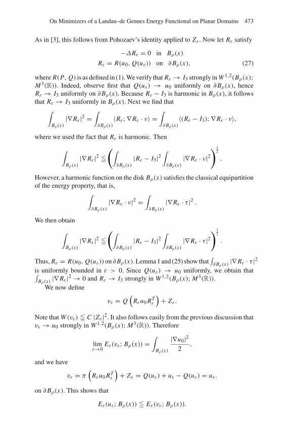
As in [3], this follows from Pohozaev’s identity applied to Zε. Now let Rε satisfy
−ΔRε = 0 in Bρ(x)
Rε = R(u0, Q(uε)) on ∂Bρ(x), (27)
where R(P, Q) is as defined in (1). We verify that Rε → I3 strongly in W 1,2(Bρ(x);M3(R)). Indeed, observe first that Q(uε) → u0 uniformly on ∂Bρ(x), henceRε → I3 uniformly on ∂Bρ(x). Because Rε − I3 is harmonic in Bρ(x), it followsthat Rε → I3 uniformly in Bρ(x). Next we find that
∫Bρ(x)
|∇ Rε|2 =∫∂Bρ(x)
〈Rε; ∇ Rε · ν〉 =∫∂Bρ(x)
〈(Rε − I3); ∇ Rε · ν〉,
where we used the fact that Rε is harmonic. Then
∫Bρ(x)
|∇ Rε|2 �(∫
∂Bρ(x)|Rε − I3|2
∫∂Bρ(x)
|∇ Rε · ν|2) 1
2
.
However, a harmonic function on the disk Bρ(x) satisfies the classical equipartitionof the energy property, that is,
∫∂Bρ(x)
|∇ Rε · ν|2 =∫∂Bρ(x)
|∇ Rε · τ |2 .
We then obtain
∫Bρ(x)
|∇ Rε|2 �(∫
∂Bρ(x)|Rε − I3|2
∫∂Bρ(x)
|∇ Rε · τ |2) 1
2
.
Thus, Rε = R(u0, Q(uε))on ∂Bρ(x). Lemma 1 and (25) show that∫∂Bρ(x)
|∇ Rε · τ |2is uniformly bounded in ε > 0. Since Q(uε) → u0 uniformly, we obtain that∫
Bρ(x)|∇ Rε|2 → 0 and Rε → I3 strongly in W 1,2(Bρ(x); M3(R)).
We now define
vε = Q(
Rεu0 RTε
)+ Zε.
Note that W (vε) � C |Zε|2. It also follows easily from the previous discussion thatvε → u0 strongly in W 1,2(Bρ(x); M3(R)). Therefore
limε→0
Eε(vε; Bρ(x)) =∫
Bρ(x)
|∇u0|22
,
and we have
vε = π(
Rεu0 RTε
)+ Zε = Q(uε)+ uε − Q(uε) = uε.
on ∂Bρ(x). This shows that
Eε(uε; Bρ(x)) � Eε(vε; Bρ(x)).
474 Dmitry Golovaty & José Alberto Montero
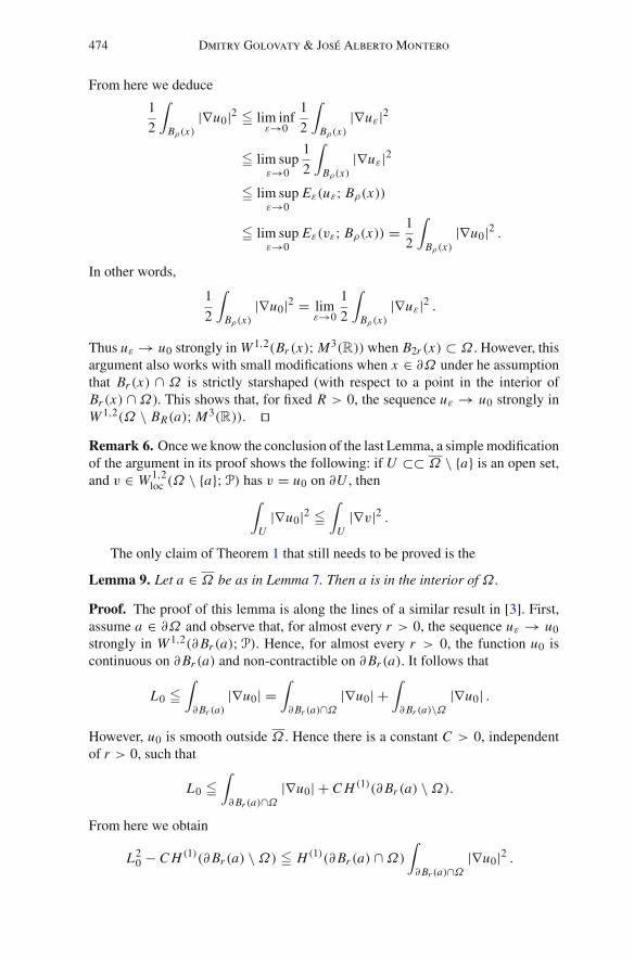
From here we deduce
1
2
∫Bρ(x)
|∇u0|2 � lim infε→0
1
2
∫Bρ(x)
|∇uε|2
� lim supε→0
1
2
∫Bρ(x)
|∇uε|2
� lim supε→0
Eε(uε; Bρ(x))
� lim supε→0
Eε(vε; Bρ(x)) = 1
2
∫Bρ(x)
|∇u0|2 .
In other words,
1
2
∫Bρ(x)
|∇u0|2 = limε→0
1
2
∫Bρ(x)
|∇uε|2 .
Thus uε → u0 strongly in W 1,2(Br (x); M3(R))when B2r (x) ⊂ Ω . However, thisargument also works with small modifications when x ∈ ∂Ω under he assumptionthat Br (x) ∩ Ω is strictly starshaped (with respect to a point in the interior ofBr (x) ∩Ω). This shows that, for fixed R > 0, the sequence uε → u0 strongly inW 1,2(Ω \ BR(a); M3(R)). ��Remark 6. Once we know the conclusion of the last Lemma, a simple modificationof the argument in its proof shows the following: if U ⊂⊂ Ω \ {a} is an open set,and v ∈ W 1,2
loc (Ω \ {a};P) has v = u0 on ∂U , then∫
U|∇u0|2 �
∫U
|∇v|2 .
The only claim of Theorem 1 that still needs to be proved is the
Lemma 9. Let a ∈ Ω be as in Lemma 7. Then a is in the interior of Ω .
Proof. The proof of this lemma is along the lines of a similar result in [3]. First,assume a ∈ ∂Ω and observe that, for almost every r > 0, the sequence uε → u0strongly in W 1,2(∂Br (a);P). Hence, for almost every r > 0, the function u0 iscontinuous on ∂Br (a) and non-contractible on ∂Br (a). It follows that
L0 �∫∂Br (a)
|∇u0| =∫∂Br (a)∩Ω
|∇u0| +∫∂Br (a)\Ω
|∇u0| .
However, u0 is smooth outside Ω . Hence there is a constant C > 0, independentof r > 0, such that
L0 �∫∂Br (a)∩Ω
|∇u0| + C H (1)(∂Br (a) \Ω).
From here we obtain
L20 − C H (1)(∂Br (a) \Ω) � H (1)(∂Br (a) ∩Ω)
∫∂Br (a)∩Ω
|∇u0|2 .
On Minimizers of a Landau–de Gennes Energy Functional on Planar Domains 475
Then
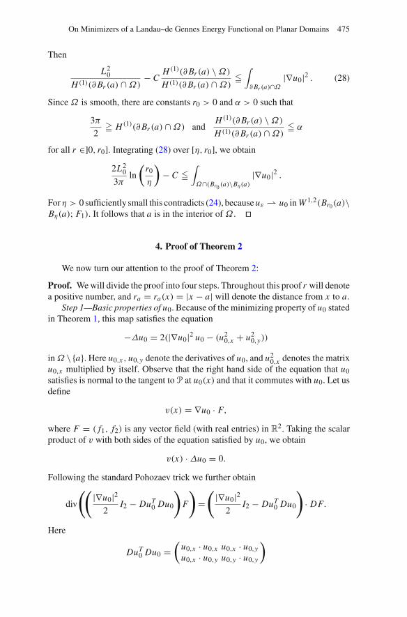
L20
H (1)(∂Br (a) ∩Ω) − CH (1)(∂Br (a) \Ω)H (1)(∂Br (a) ∩Ω) �
∫∂Br (a)∩Ω
|∇u0|2 . (28)
Since Ω is smooth, there are constants r0 > 0 and α > 0 such that
3π
2� H (1)(∂Br (a) ∩Ω) and
H (1)(∂Br (a) \Ω)H (1)(∂Br (a) ∩Ω) � α
for all r ∈]0, r0]. Integrating (28) over [η, r0], we obtain
2L20
3πln
(r0
η
)− C �
∫Ω∩(Br0 (a)\Bη(a)
|∇u0|2 .
Forη > 0 sufficiently small this contradicts (24), because uε ⇀ u0 in W 1,2(Br0(a)\Bη(a); F1). It follows that a is in the interior of Ω . ��
4. Proof of Theorem 2
We now turn our attention to the proof of Theorem 2:
Proof. We will divide the proof into four steps. Throughout this proof r will denotea positive number, and ra = ra(x) = |x − a| will denote the distance from x to a.
Step 1—Basic properties of u0. Because of the minimizing property of u0 statedin Theorem 1, this map satisfies the equation
−Δu0 = 2(|∇u0|2 u0 − (u20,x + u2
0,y))
inΩ \ {a}. Here u0,x , u0,y denote the derivatives of u0, and u20,x denotes the matrix
u0,x multiplied by itself. Observe that the right hand side of the equation that u0satisfies is normal to the tangent to P at u0(x) and that it commutes with u0. Let usdefine
v(x) = ∇u0 · F,
where F = ( f1, f2) is any vector field (with real entries) in R2. Taking the scalar
product of v with both sides of the equation satisfied by u0, we obtain
v(x) ·Δu0 = 0.
Following the standard Pohozaev trick we further obtain
div
((|∇u0|2
2I2 − DuT
0 Du0
)F
)=(
|∇u0|22
I2 − DuT0 Du0
)· DF.
Here
DuT0 Du0 =
(u0,x · u0,x u0,x · u0,yu0,x · u0,y u0,y · u0,y
)
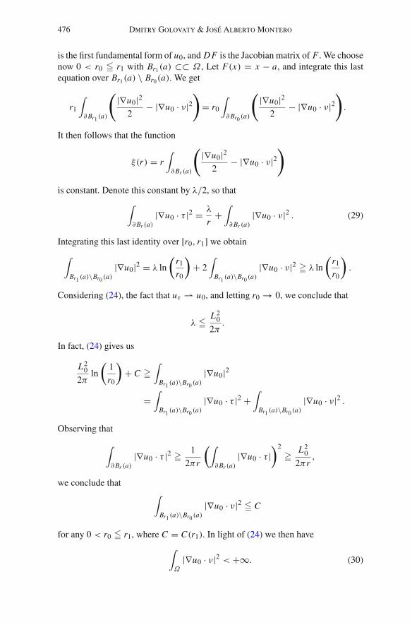
476 Dmitry Golovaty & José Alberto Montero
is the first fundamental form of u0, and DF is the Jacobian matrix of F . We choosenow 0 < r0 � r1 with Br1(a) ⊂⊂ Ω , Let F(x) = x − a, and integrate this lastequation over Br1(a) \ Br0(a). We get
r1
∫∂Br1 (a)
(|∇u0|2
2− |∇u0 · ν|2
)= r0
∫∂Br0 (a)
(|∇u0|2
2− |∇u0 · ν|2
).
It then follows that the function
ξ(r) = r∫∂Br (a)
(|∇u0|2
2− |∇u0 · ν|2
)
is constant. Denote this constant by λ/2, so that∫∂Br (a)
|∇u0 · τ |2 = λ
r+∫∂Br (a)
|∇u0 · ν|2 . (29)
Integrating this last identity over [r0, r1] we obtain
∫Br1 (a)\Br0 (a)
|∇u0|2 = λ ln
(r1
r0
)+ 2
∫Br1 (a)\Br0 (a)
|∇u0 · ν|2 � λ ln
(r1
r0
).
Considering (24), the fact that uε ⇀ u0, and letting r0 → 0, we conclude that
λ � L20
2π.
In fact, (24) gives us
L20
2πln
(1
r0
)+ C �
∫Br1 (a)\Br0 (a)
|∇u0|2
=∫
Br1 (a)\Br0 (a)|∇u0 · τ |2 +
∫Br1 (a)\Br0 (a)
|∇u0 · ν|2 .
Observing that
∫∂Br (a)
|∇u0 · τ |2 � 1
2πr
(∫∂Br (a)
|∇u0 · τ |)2
� L20
2πr,
we conclude that ∫Br1 (a)\Br0 (a)
|∇u0 · ν|2 � C
for any 0 < r0 � r1, where C = C(r1). In light of (24) we then have∫Ω
|∇u0 · ν|2 < +∞. (30)
On Minimizers of a Landau–de Gennes Energy Functional on Planar Domains 477
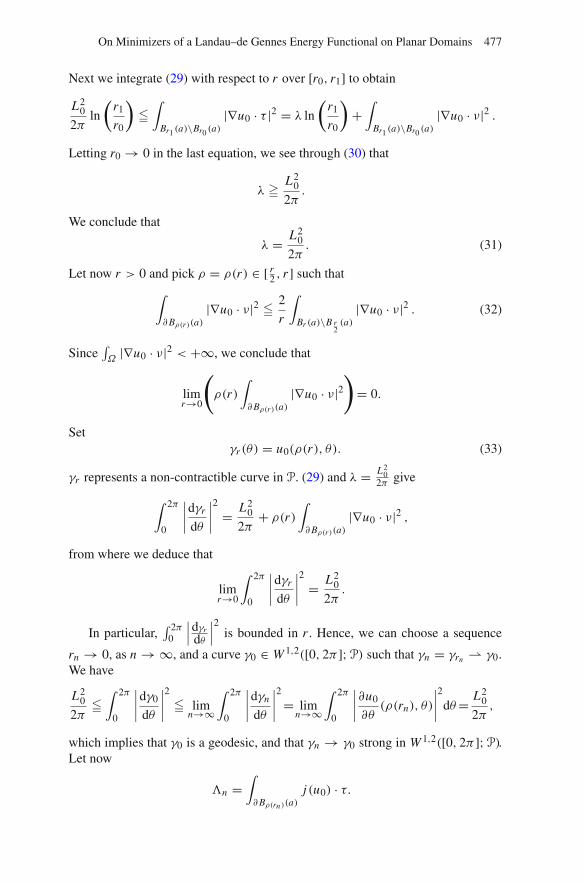
Next we integrate (29) with respect to r over [r0, r1] to obtain
L20
2πln
(r1
r0
)�∫
Br1 (a)\Br0 (a)|∇u0 · τ |2 = λ ln
(r1
r0
)+∫
Br1 (a)\Br0 (a)|∇u0 · ν|2 .
Letting r0 → 0 in the last equation, we see through (30) that
λ � L20
2π.
We conclude that
λ = L20
2π. (31)
Let now r > 0 and pick ρ = ρ(r) ∈ [ r2 , r ] such that
∫∂Bρ(r)(a)
|∇u0 · ν|2 � 2
r
∫Br (a)\B r
2(a)
|∇u0 · ν|2 . (32)
Since∫Ω
|∇u0 · ν|2 < +∞, we conclude that
limr→0
(ρ(r)
∫∂Bρ(r)(a)
|∇u0 · ν|2)
= 0.
Setγr (θ) = u0(ρ(r), θ). (33)
γr represents a non-contractible curve in P. (29) and λ = L20
2π give
∫ 2π
0
∣∣∣∣dγr
dθ
∣∣∣∣2
= L20
2π+ ρ(r)
∫∂Bρ(r)(a)
|∇u0 · ν|2 ,
from where we deduce that
limr→0
∫ 2π
0
∣∣∣∣dγr
dθ
∣∣∣∣2
= L20
2π.
In particular,∫ 2π
0
∣∣∣dγr
dθ
∣∣∣2 is bounded in r . Hence, we can choose a sequence
rn → 0, as n → ∞, and a curve γ0 ∈ W 1,2([0, 2π ];P) such that γn = γrn ⇀ γ0.We have
L20
2π�∫ 2π
0
∣∣∣∣dγ0
dθ
∣∣∣∣2
� limn→∞
∫ 2π
0
∣∣∣∣dγn
dθ
∣∣∣∣2
= limn→∞
∫ 2π
0
∣∣∣∣∂u0
∂θ(ρ(rn), θ)
∣∣∣∣2
dθ= L20
2π,
which implies that γ0 is a geodesic, and that γn → γ0 strong in W 1,2([0, 2π ];P).Let now
�n =∫∂Bρ(rn )(a)
j (u0) · τ.
478 Dmitry Golovaty & José Alberto Montero
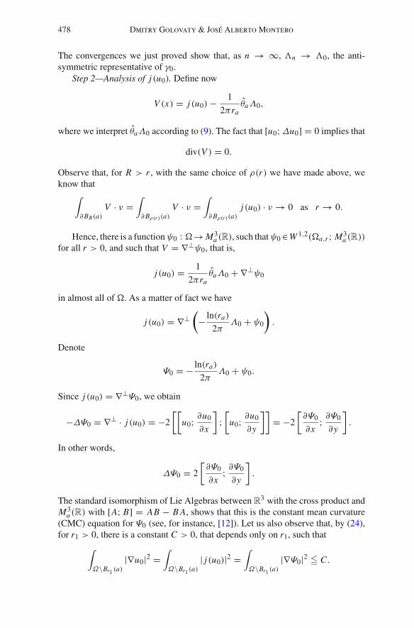
The convergences we just proved show that, as n → ∞, �n → �0, the anti-symmetric representative of γ0.
Step 2—Analysis of j (u0). Define now
V (x) = j (u0)− 1
2πraθ̂aΛ0,
where we interpret θ̂aΛ0 according to (9). The fact that [u0;Δu0] = 0 implies that
div(V ) = 0.
Observe that, for R > r , with the same choice of ρ(r) we have made above, weknow that∫
∂BR(a)V · ν =
∫∂Bρ(r)(a)
V · ν =∫∂Bρ(r)(a)
j (u0) · ν → 0 as r → 0.
Hence, there is a functionψ0 : �→ M3a (R), such thatψ0 ∈W 1,2(�a,r ; M3
a (R))
for all r > 0, and such that V = ∇⊥ψ0, that is,
j (u0) = 1
2πraθ̂aΛ0 + ∇⊥ψ0
in almost all of �. As a matter of fact we have
j (u0) = ∇⊥(
− ln(ra)
2πΛ0 + ψ0
).
Denote
Ψ0 = − ln(ra)
2πΛ0 + ψ0.
Since j (u0) = ∇⊥Ψ0, we obtain
−ΔΨ0 = ∇⊥ · j (u0) = −2
[[u0; ∂u0
∂x
];[
u0; ∂u0
∂y
]]= −2
[∂Ψ0
∂x; ∂Ψ0
∂y
].
In other words,
ΔΨ0 = 2
[∂Ψ0
∂x; ∂Ψ0
∂y
].
The standard isomorphism of Lie Algebras between R3 with the cross product and
M3a (R) with [A; B] = AB − B A, shows that this is the constant mean curvature
(CMC) equation for Ψ0 (see, for instance, [12]). Let us also observe that, by (24),for r1 > 0, there is a constant C > 0, that depends only on r1, such that
∫Ω\Br1 (a)
|∇u0|2 =∫Ω\Br1 (a)
| j (u0)|2 =∫Ω\Br1 (a)
|∇Ψ0|2 � C.
On Minimizers of a Landau–de Gennes Energy Functional on Planar Domains 479
The proof of the regularity of the solutions of the CMC equation, as shown forinstance in [12], shows then that Ψ0 is smooth in Ω \ Br1(a). However, it is easyto see that
∫Ω
|∇Ψ0|2 = +∞.
In other words, we cannot apply the known results regarding regularity of solutionsof the CMC equation to Ψ0 in the whole of Ω .
Step 3—Analysis of Ψ0. Now we show that
ψ0 = Ψ0 + ln(ra)
2πΛ0,
satisfies ψ0 ∈ W 1,2(Ω; M3a (R)), and also
Δψ0 = 2
[∂ψ0
∂x; ∂ψ0
∂y
]+ 1
πra
[∇ψ0 · θ̂a;Λ0
].
This, plus some extra work, will give us that ψ0 ∈ L∞(Ω; M3a (R)). To this end let
us observe that
j (u0) = θ̂a
2πraΛ0 + ∇⊥ψ0.
In particular,
∫Ω
∣∣∣∇ψ0 · θ̂a
∣∣∣2 =∫Ω
∣∣ j (u0) · r̂a∣∣2 < +∞.
Next, a direct computation shows that
Δψ0 = ∇⊥ · j (ψ0)+ 1
πra[∇ψ0 · θ̂a;Λ0].
Dotting this equation into φ = ∇ψ0 · B, for B(x) = x − a, and following thestandard Pohozaev’s identity trick, we arrive at
div
((|∇ψ0|2
2I2 − DψT
0 Dψ0
)B
)= − 1
πΛ0 · [∇ψ0 · r̂a; ∇ψ0 · θ̂a]
= − 1
2πΛ0 ·
(∇⊥ · j (ψ)
).
At the end of Step 1, we had found a sequence rn → 0 as n → ∞, with acorresponding ρ(rn) from (32), such that
480 Dmitry Golovaty & José Alberto Montero
γn(θ) = u0(ρ(rn), θ) → γ0 strongly in W 1,2([0, 2π ];P).
We pick an arbitrary r > 0 with Br (a) ⊂ Ω , any n such that rn < r , and integratethe equation at the top of the page over Br (a)\Bρ(rn)(a). Since�0 is constant, andwriting ρn instead of ρ(rn), we obtain
r∫∂Br (a)
(|∇ψ0|2
2− |∇ψ0 · ν|2
)− ρn
∫∂Bρn (a)
(|∇ψ0|2
2− |∇ψ0 · ν|2
)
= −Λ0
2π·∫
Br (a)\Bρn (a)∇⊥ · j (ψ0)
= −Λ0
2π·∫∂(Br (a)\Bρn (a))
j (ψ0) · τ. (34)
Let us recall now that
j (u0) = θ̂a
2πraΛ0 + ∇⊥ψ0.
This says that
ρn
∫∂Bρn (a)
|∇ψ0 · ν|2 = ρn
∫∂Bρn (a)
∣∣∣∣∣(
j (u0)− θ̂a
2πraΛ0
)· τ∣∣∣∣∣2
=∫ 2π
0
∣∣∣∣[γn; dγn
dθ
]− 1
2πΛ0
∣∣∣∣2
→ 0
as n → ∞.Next, the definition of j (u0) shows that
ρn
∫∂Bρn (a)
|∇ψ0 · τ |2 = ρn
∫∂Bρn (a)
|∇u0 · ν|2 .
By (32),
ρn
∫∂Bρn (a)
|∇ψ0 · τ |2 → 0
as n → ∞.Now observe that, if A ∈ M3
a (R) is constant over ∂Bρn (a), then
∫∂Bρn (a)
[A; ∇ψ0 · τ ] =[
A;∫∂Bρn (a)
∇ψ0 · τ]
= 0
because ∂Bρn (a) is a closed curve. We use this with A = ψρn0 = ψ0(xρn ) for some
fixed xρn ∈ ∂Bρn (a), to obtain∫∂Bρn (a)
j (ψ0) · τ =∫∂Bρn (a)
[ψ0; ∇ψ0 · τ ] =∫∂Bρn (a)
[ψ0 − ψ
ρn0 ; ∇ψ0 · τ ] .
(35)
On Minimizers of a Landau–de Gennes Energy Functional on Planar Domains 481
Let x ∈ ∂Bρn (a) and call �(xρn , x) the connected portion of ∂Bρn (a) that starts atxρn and ends at x . Obviously
ψ0(x)− ψρn0 =
∫�(xρn ,x)
∇ψ0 · τ.
Using this in (35) we obtain
∣∣∣∣∣∫∂Bρn (a)
j (ψ0) · τ∣∣∣∣∣ �
(∫∂Bρn (a)
|∇ψ0 · τ |)2
� 2πρn
∫∂Bρn (a)
|∇ψ0 · τ |2 . (36)
We conclude that ∣∣∣∣∣∫∂Bρn (a)
j (ψ0) · τ∣∣∣∣∣ → 0
as n → ∞. With all these facts we go back to (34) and let n → ∞ to obtain
r∫∂Br (a)
(|∇ψ0|2
2− |∇ψ0 · ν|2
)= −Λ0
2π·∫∂Br (a)
j (ψ0) · τ. (37)
This is valid for any r > 0 such that Br (a) ⊂ �.Observe now that the argument we used to obtain (36) can be applied to any
r > 0 with Br (a) ⊂ �. We use this on the right-hand side of (37) to obtain∫∂Br (a)
|∇ψ0 · ν|2 � C∫∂Br (a)
|∇ψ0 · τ |2 ,
where C depends on �0, but is independent of r > 0. We recall now that∫Ω
|∇u0 · ν|2 < +∞.
This implies that∫
Br (a)|∇ψ0 · τ |2
is finite, and hence∫
Br (a)|∇ψ0|2
is also finite.Once we know that ψ0 ∈ W 1,2(Ω; M3
a (R)), the last assertion of Theorem 2can be proved as follows. First notice that
u0∂u0
∂xu0 = u0
∂u0
∂yu0 = 0,
482 Dmitry Golovaty & José Alberto Montero
because u0 is P-valued. From here we obtain that[
u0; ∂u0
∂x
]= u0
[u0; ∂u0
∂x
]+[
u0; ∂u0
∂x
]u0,
and the same holds for ∂u0∂y . This last identity, the fact that
j (u0) = 1
2πra(Λ0θ̂a)+ ∇⊥ψ0,
and some algebra show that
Zu0(x) = 1
2πra(Λ0 − u0Λ0 −Λ0u0)
also satisfies
Zu0(x) = −((∇⊥ψ0 · θ̂a)− u0(∇⊥ψ0 · θ̂a)− (∇⊥ψ0 · θ̂a)u0).
Since ψ0 ∈ W 1,2(Ω; M3a (R)), it follows that Zu0 ∈ L2(Ω; M3
a (R)).Step 4—Proof of the fact that ψ0 ∈ L∞(Ω; M3
a (R)). From all we have done sofar it is clear that ψ0 is bounded, and in fact smooth, away from a. All we need isto analyze ψ0 near a. To do this, recall that
∫Ω
|∇ψ0|2
is finite. Hence, by adding a constant to ψ0 we can also impose that∫Ω
|ψ0|2
be finite. In particular we have that
limδ→0
∫Bδ(a)
(|∇ψ0|2 + |ψ0|2) = 0.
Now, for any δ > 0 we can choose η = η(δ) ∈ [δ/2, δ] such that∫∂Bη(a)
(|∇ψ0|2 + |ψ0|2) � 2
δ
∫(Bδ\Bδ/2)(a)
(|∇ψ0|2 + |ψ0|2)
Notice that(∫
∂Bη(a)(|∇ψ0| + |ψ0|)
)2
� C∫(Bδ\Bδ/2)(a)
(|∇ψ0|2 + |ψ0|2),
and hence
limδ→0
∫∂Bη(a)
(|∇ψ0| + |ψ0|) = 0.
On Minimizers of a Landau–de Gennes Energy Functional on Planar Domains 483
Let us choose now R > 0 such that B4R(a) ⊂ Ω , and pick b ∈ BR(a), b = a. Letalso δ > 0 be small, and set
Uδ = B2R(b) \ (Bη(a) ∪ Bη(b)),
where η = η(δ) is as explained before. Call
G(x, y) = 1
2πln
(1
|x − y|),
the fundamental solution of the Laplacian in the plane. Observe now that, awayfrom a, we have
Δψ0 = 2
[∂ψ0
∂x; ∂ψ0
∂y
]+ 1
πra
[∇ψ0 · θ̂a;Λ0
]
= ∇⊥ · j (ψ0)+ div
(θ̂a
πra[ψ0;Λ0]
)
Using Green’s identity we obtain∫∂Uδ(G(b, y)∇ψ0 − ψ0∇G(b, y)) · ν
=∫
UδG(b, y)
(∇⊥ · j (ψ0)+ div
(θ̂a
πra[ψ0;Λ0]
))
= −∫
Uδ
(θ̂b
2πrb· j (ψ0)− r̂b · θ̂a
π2rarb[ψ0;Λ0]
)
+∫∂Uδ
G(b, y)τ · j (ψ0)+∫∂Uδ
ν · θ̂a
πra[ψ0;Λ0] . (38)
We intend to let δ → 0 in this last identity. To do this, observe that∫∂Bη(a)
ν · θ̂a
πra[ψ0;Λ0] = 0,
and, since ψ0 is smooth at b,
limδ→0
∫∂Bη(b)
ν · θ̂a
πra[ψ0;Λ0] = 0.
Using again that ψ0 is smooth away from a,we obtain
limδ→0
∫∂Bη(b)
G(b, y)τ · j (ψ0) = 0.
Now, if ψη0 = ψ0(xη) for a fixed xη ∈ ∂Bη(a), and, for x ∈ ∂Bη(a), �(xη, x) isthe shortest portion of ∂Bη(a) that starts in xη and ends in x , then
ψ0(x)− ψη0 =
∫�(xη,x)
∇ψ0 · τ,
484 Dmitry Golovaty & José Alberto Montero
so that
∣∣ψ0(x)− ψη0
∣∣ �∫∂Bη(a)
|∇ψ0| .
Writing∫∂Bη(a)
G(b, y)τ · j (ψ0) =∫∂Bη(a)
(G(b, y)− G(b, a)τ · j (ψ0)
+ G(b, a)∫∂Bη(a)
τ · j (ψ0),
we estimate∣∣∣∣∣∫∂Bη(a)
τ · j (ψ0)
∣∣∣∣∣ =∣∣∣∣∣∫∂Bη(a)
[ψ0 − ψτ0 ; ∇ψ0 · τ ]
∣∣∣∣∣
�(∫
∂Bη(a)|∇ψ0|
)2
� 2πη∫∂Bη(a)
|∇ψ0|2 → 0,
by the choice of η. Again, this choice gives us that∣∣∣∣∣∫∂Bη(a)
(G(b, y)− G(b, a)τ · j (ψ0)
∣∣∣∣∣ � C(a, b)δ∫∂Bη(a)
|ψ0| |∇ψ0| → 0
as δ → 0 as well.We notice next that, because a = b, 1
rarb∈ L p(Ω) for any p < 2. Since
ψ0 ∈ W 1,2(Ω), we obtain that
r̂b · θ̂a
π2rarb[ψ0;Λ0] ∈ L1(Ω).
Observe now that G(b, y) is smooth near a, while ψ0 is smooth near b. Because ofthis, and the choice of η, we conclude that
limδ→0
∫∂Bη(a)
G(b, y) |∇ψ0| = limδ→0
∫∂Bη(b)
G(b, y) |∇ψ0| = 0.
Using again that G(b, y) is smooth near a and ψ0 is smooth near b we concludethat
limδ→0
∫∂Bη(a)
ψ0∇G(b, y)) · ν = 0,
and
limδ→0
∫∂Bη(b)
ψ0∇G(b, y)) · ν = −ψ(b).
On Minimizers of a Landau–de Gennes Energy Functional on Planar Domains 485
Now we observe that, for r > η > 0 and r small but fixed,
∫(Br \Bη)(b)
θ̂b
2πrb· j (ψ0) =
∫ r
η
1
2πrb
(∫∂Bs (b)
j (ψ0) · θ̂b
)ds.
By the argument we gave to go from (35) to (36), this integral is bounded by∫Ω
|∇ψ0|2. Putting all of this together in (38), as δ → 0 we obtain
ψ0(b) = −∫∂B2R(b)
(G(b, y)∇ψ0 − ψ0∇G(b, y)) · ν
−∫
B2R(b)
(θ̂b
2πrb· j (ψ0)+ r̂b · θ̂a
π2rarb[ψ0;Λ0]
)
+∫∂B2R(b)
G(b, y)τ · j (ψ0)+∫∂B2R(b)
ν · θ̂a
πra[ψ0;Λ0] . (39)
By the choice of R, because b ∈ BR(a) and becauseψ0 is smooth away from a, theboundary integrals above are uniformly bounded in b. Next, we already mentionedthat the term
∫B2R(b)
θ̂b
2πrb· j (ψ0)
can be bounded by∫Ω
|∇ψ0|2 .
Finally we need to estimate
∫B2R(b)
r̂b · θ̂a
rarb[ψ0;Λ0] .
For simplicity let us consider the case b = (0, 0), and a = (λ, 0). Then
r̂b = 1
rb(x, y) and θ̂a = 1
ra(−y, x − λ),
so that∫
B2R(b)
r̂b · θ̂a
rarb[ψ0;Λ0] = −λ
∫B2R(b)
y
r2a r2
b
[ψ0;Λ0] .
Write now B+2R(b) = {(x, y) ∈ B2R(b) : y � 0}. Then
∫B2R(b)
r̂b · θ̂a
rarb[ψ0;Λ0] = − λ
∫B+
2R(b)
y
r2a r2
b
([ψ0(x, y);Λ0] − [ψ0(x,−y);Λ0])
= − λ
∫B+
2R(b)
y
r2a r2
b
([ψ0(x, y);Λ0] − [ψ0(x, 0);Λ0])
486 Dmitry Golovaty & José Alberto Montero
− λ
∫B+
2R(b)
y
r2a r2
b
([ψ0(x,−y);Λ0] − [ψ0(x, 0);Λ0]) .
We estimate the first of these two integrals, as the second obviously can be estimatedin the same manner. To do this observe that
− λ
∫B+
2R(b)
y
r2a r2
b
([ψ0(x, y);Λ0] − [ψ0(x, 0);Λ0])
= −λ∫ 2R
−2R
∫ √2R2−x2
0
y
r2a r2
b
[∫ y
0
∂ψ0
∂y(x, s) ds;Λ0
]dy dx
= −λ∫ 2R
−2R
∫ √4R2−x2
0
[∂ψ0
∂y(x, s);Λ0
] ∫ √4R2−x2
s
y
r2a r2
b
dy ds dx
Note next that∫ √
4R2−x2
s
y
r2a r2
b
=∫ √
4R2−x2
s
y
((x − λ)2 + y2)(x2 + y2)
=∫ √
4R2−x2
s
(1
x2 + y2 − 1
(x − λ)2 + y2
)y dy
λ2 − 2λx
= 1
2(λ2 − 2λx)
(ln
(4R2
x2 + s2
)− ln
(λ2 − 2λx + 4R2
(x − λ)2 + s2
))
= 1
2(λ2 − 2λx)
(ln
((x − λ)2 + s2
x2 + s2
)−ln
(λ2−2λx + 4R2
4R2
))
Let us recall now the elementary estimate |ln(1 + t)| � C |t |, valid for |t | � 1/2.This says that, if
∣∣λ2 − 2xλ∣∣ � 2R2, then
∣∣∣∣ 1
2(λ2 − 2λx)ln
(λ2 − 2λx + 4R2
4R2
)∣∣∣∣ � C
R2
On the other hand, if∣∣λ2 − 2xλ
∣∣ � 2R2, then∣∣∣∣ 1
2(λ2 − 2λx)ln
(λ2 − 2λx + 4R2
4R2
)∣∣∣∣ � 1
2R2
∣∣∣∣ln(λ2 − 2λx + 4R2
4R2
)∣∣∣∣ .All this shows that∣∣∣∣∣
1
2(λ2 − 2λx)
∫ 2R
−2R
∫ √4R2−x2
0
[∂ψ0
∂y(x, s);Λ0
]ln
(λ2 − 2λx + 4R2
4R2
)∣∣∣∣∣� C
R2
∫B2R
∣∣∣∣∂ψ0
∂y(x, s)
∣∣∣∣max
{1;∣∣∣∣ln
(λ2 − 2λx + 4R2
4R2
)∣∣∣∣},
and the last integral is controlled by∫Ω
|∇ψ0|2.We are left only with the integral
I =∫
B2R
[∂ψ0
∂y(x, s);Λ0
]λ
(λ2 − 2λx)ln
((x − λ)2 + s2
x2 + s2
)ds dx .
On Minimizers of a Landau–de Gennes Energy Functional on Planar Domains 487
Now by Holder’s inequality
|I | � C
(∫B2R
|∇ψ0|2∫
B2R
λ2
(λ2 − 2λx)2ln2
((x − λ)2 + s2
x2 + s2
))1/2
.
We need then to estimate∫
B2R
λ2
(λ2 − 2λx)2ln2
((x − λ)2 + s2
x2 + s2
)�∫
R2
1
(λ− 2x)2ln2
((x − λ)2 + s2
x2 + s2
)
= 1
4
∫R2
1
x2 ln2
((x − λ
2 )2 + s2
(x + λ2 )
2 + s2
)
A simple way to see that this last integral is finite is to introduce bipolar coordinates,with poles at (−λ
2 , 0) and ( λ2 , 0). These coordinates are
τ = ln
((x − λ
2 )2 + s2
(x + λ2 )
2 + s2
)
and the angle (−λ2 , 0)− (x, y)− ( λ2 , 0), that we denote σ . With these coordinates,
x = λ sinh(τ )
cosh(τ )− cos(σ )
and
dx ds = λ2
(cosh(τ )− cos(σ ))2.
Then∫
R2
1
x2 ln2
((x − λ
2 )2 + s2
(x + λ2 )
2 + s2
)=∫ 2π
0
∫ ∞
−∞τ 2
sinh2(τ )dτ dσ =2π
∫ ∞
−∞τ 2
sinh2(τ )dτ,
which is clearly finite. ��
Appendix
Here we provide an alternative argument to Lemma 2 demonstrating that thecritical points of a slightly more general version of Eε take values in the convexhull of P as long as their boundary data is in P.
Lemma 10. For any critical point uε ∈ W 1,2(Ω; F1) of the functional
Eβε (u) =∫Ω
(|∇u|2
2+ Wβ(u)
ε2
),
such that u|∂Ω ∈ P, the function uε takes values in the convex hull of P.
488 Dmitry Golovaty & José Alberto Montero
Proof. We divide the proof into two steps.Step 1. The potential Wβ defined in (4) can be written as
Wβ(u) = 1
2(1 − |u|2)2 − β
6(1 − 3 |u|2 + 2tr(u3)),
where |u|2 = tr u2. The gradient of the potential is
(∇u Wβ)(u) = 2(|u|2 − 1)u + β(u − u2),
and its trace is
tr(∇u Wβ)(u) = (β − 2)(1 − |u|2).We first compute the inner product
〈u; (∇u Wβ)(u)〉 = 2(|u|2 − 1) |u|2 + β(|u|2 − tr(u3)),
and rewrite this expression as follows
〈u; (∇u Wβ)(u)〉 = 2(|u|2 − 1)2 + 2(|u|2 − 1)+ β(|u|2 − tr(u3)).
Then
〈u; (∇u Wβ)(u)〉 = 2(|u|2 − 1)2 − β
2(1 − 3 |u|2 + 2tr(u3))
+ (|u|2 − 1)
(2 − β
2
).
Comparing this with the definition of Wβ we obtain
〈u; (∇u Wβ)(u)〉 = 4W 3β4
+ (|u|2 − 1)
(2 − β
2
).
For critical points of
Eβε (u) =∫Ω
(|∇u|2
2+ Wβ(u)
ε2
)
in F1, we have
−Δu + 1
ε2 (∇u Wβ)(u) = λI3,
where the Lagrange multiplier
λ = (β − 2)(1 − |u|2)3
.
Now set
α := |u|22.
On Minimizers of a Landau–de Gennes Energy Functional on Planar Domains 489
The computations above show that
Δα = |∇u|2 + 〈u; (∇u Wβ)(u)〉 − (β − 2)(1 − |u|2)3
= |∇u|2 + 1
ε2
(4W 3β
4+ (|u|2 − 1)
(2 + β − 2
3− β
2
)).
In other words,
Δα = |∇u|2 + 1
ε2
(4W 3β
4+ 8 − β
6(|u|2 − 1)
).
A standard maximum principle argument then shows that |u| � 1 when β � 8.Step 2. We now follow the same line of reasoning for τ = 〈u; P〉, where P ∈P
is a constant projection matrix. We observe that
Δτ = 〈Δu; P〉 = 1
ε2
(2(|u|2 − 1)τ + βτ − β〈u2; P〉 − (β − 2)(1 − |u|2)
3
).
If we write u in terms of its eigenvalues and eigenvectors as u = ∑nk=1 λk Pk , then∑3
k=1〈P; Pk〉 = 1 and 〈P; Pk〉 � 0 for all k = 1, . . . , 3. By Jensen’s inequality
τ 2 =(
3∑k=1
λk〈Pk; P〉)2
�3∑
k=1
λ2k〈Pk; P〉 = 〈u2; P〉.
Let us assume now 8 � β > 2. Then |u| � 1 from Step 1, and from the lastinequality we obtain
Δτ � β
ε2
(1 − 2
β(1 − |u|2)− τ
)τ.
Set ξ = 1 − τ . Then ξ has
Δξ � (ξ − 1)
(ξ − 2
β(1 − |u|2)
).
In particular, if Ω> = {x ∈ Ω : ξ(x) > 1}, the function ξ is subharmonic in Ω>.Since on ∂Ω we have ξ = 1 − 〈u; P〉 � 1, ifΩ> were nonempty (and also open),ξ would attain a maximum in its interior. By the maximum principle ξ would beconstant in Ω>—a contradiction. We conclude that ξ � 1 in Ω .
Since ξ = 1 − 〈u; P〉 � 1 in Ω , we conclude that
〈u; P〉 � 0
for all P ∈ P fixed. Therefore, when β > 2, the critical points uε of Eε have λ3 � 0and uε takes values in the convex hull of P. ��
490 Dmitry Golovaty & José Alberto Montero
References
1. Ball, J.M., Zarnescu, A.: Orientability and energy minimization in liquid crystalmodels. Arch. Ration. Mech. Anal. 202(2), 493–535 (2011). doi:10.1007/s00205-011-0421-3
2. Bauman, P., Park, J., Phillips, D.: Analysis of nematic liquid crystals with disclinationlines. Arch. Ration. Mech. Anal. 205(3), 795–826 (2012). doi:10.1007/s00205-012-0530-7
3. Bethuel, F., Brezis, H., Hélein, F.: Ginzburg–Landau vortices. Progress in NonlinearDifferential Equations and Their Applications, vol. 13. Birkhäuser Boston Inc., Boston,(1994). doi:10.1007/978-1-4612-0287-5
4. Canevari, G.: Biaxiality in the asymptotic analysis of a 2-D Landau–de Gennes modelfor liquid crystals. ArXiv e-prints (2013)
5. Ericksen, J.: Liquid crystals with variable degree of orientation. Arch. Ration. Mech.Anal. 113(2), 97–120 (1991). doi:10.1007/BF00380413
6. Hélein, F., Pedit, F.: Harmonic maps, conservation laws and moving frames, JindrichNecas Center for Mathematical Modeling Lecture Notes, vol. 7. Cambridge UniversityPress, Cambridge, (2004)
7. Jerrard, R.L.: Lower bounds for generalized Ginzburg–Landau functionals. SIAM J.Math. Anal. 30(4), 721–746 (1999). doi:10.1137/S0036141097300581
8. Klapicky, P. (ed.): Topics in mathematical modelling and analysis, Jindrich NecasCenter for Mathematical Modeling Lecture Notes, vol. 7. MATFYZPRESS, PublishingHouse of the Faculty of Mathematics and Physics, Charles University in Prague, Prague,(2012)
9. Majumdar, A.: Equilibrium order parameters of nematic liquid crystals in theLandau-de Gennes theory. Eur. J. Appl. Math. 21(2), 181–203 (2010). doi:10.1017/S0956792509990210
10. Majumdar, A., Zarnescu, A.: Landau–De Gennes theory of nematic liquid crystals:the Oseen–Frank limit and beyond. Arch. Ration. Mech. Anal. 196(1), 227–280 (2010).doi:10.1007/s00205-009-0249-2.
11. Mottram, N., Newton, C.: Introduction to Q-tensor theory. Tech. Rep. 10, Departmentof Mathematics, University of Strathclyde (2004)
12. Rivière, T.: Integrability by Compensation in the Analysis of Conformally InvariantProblems. Minicourse PIMS, Vancouver (2009)
13. Sandier, E.: Lower bounds for the energy of unit vector fields and applications. J.Funct. Anal. 152(2), 379–403 (1998). doi:10.1006/jfan.1997.3170.
14. Virga, E.G.: Variational theories for liquid crystals, Applied Mathematics and Mathe-matical Computation, vol. 8. Chapman & Hall, London, (1994)
Department of Mathematics, Buchtel College of Arts and Sciences,The University of Akron,Akron, OH 44325, USA.
e-mail: [email protected]
and
Departamento de Matemáticas, Facultad de Matemáticas,Pontificia Universidad Católica de Chile,
Vicuña Mackenna 4860, San Joaquín,Santiago, Chile.e-mail: [email protected]
(Received July 16, 2013 / Accepted February 27, 2014)Published online April 24, 2014 – © Springer-Verlag Berlin Heidelberg (2014)

![THE ARONSSON-EULER EQUATION FOR ABSOLUTELY ......Such minimizers are called absolutely minimizing Lipschitz extension, or absolute minimizers for short. In [1], Aronsson showed that](https://img.pdfslide.us/doc/110x75/607a00970aaae952d508037f/the-aronsson-euler-equation-for-absolutely-such-minimizers-are-called-absolutely.jpg)


![gradient in the Landau-de Gennes theory · This singular potential, called Ball-Majumdar potential, is introduced in [3], and is considered as a natural enforcement of a physical](https://img.pdfslide.us/doc/110x75/6074a0fdefe13513317e48b4/gradient-in-the-landau-de-gennes-theory-this-singular-potential-called-ball-majumdar.jpg)


![VINCENT MILLOT arXiv:0804.0128v1 [math.AP] 1 Apr …0804.0128v1 [math.AP] 1 Apr 2008 SYMMETRY OF LOCAL MINIMIZERS FOR THE THREE DIMENSIONAL GINZBURG-LANDAU FUNCTIONAL VINCENT MILLOT](https://img.pdfslide.us/doc/110x75/5ad45e887f8b9a0d2d8c4c04/vincent-millot-arxiv08040128v1-mathap-1-apr-08040128v1-mathap-1-apr.jpg)


![[Pierre-giles de Gennes] Scaling Concepts in Polymer Physics](https://img.pdfslide.us/doc/110x75/55cf860e550346484b93d57a/pierre-giles-de-gennes-scaling-concepts-in-polymer-physics.jpg)


