Autonomous Robots manuscript No.(will be inserted by the editor)

On Measuring the Accuracy of SLAM Algorithms

Rainer Kummerle · Bastian Steder ·Christian Dornhege · Michael Ruhnke ·Giorgio Grisetti · Cyrill Stachniss ·Alexander Kleiner

Received: date / Accepted: date

Abstract In this paper, we address the problem of creating an objective benchmark forevaluating SLAM approaches. We propose a framework for analyzing the results of a SLAMapproach based on a metric for measuring the error of the corrected trajectory. This metricuses only relative relations between poses and does not relyon a global reference frame. Thisovercomes serious shortcomings of approaches using a global reference frame to computethe error. Our method furthermore allows us to compare SLAM approaches that use differentestimation techniques or different sensor modalities since all computations are made basedon the corrected trajectory of the robot.

We provide sets of relative relations needed to compute our metric for an extensiveset of datasets frequently used in the robotics community. The relations have been obtainedby manually matching laser-range observations to avoid theerrors caused by matching algo-rithms. Our benchmark framework allows the user to easily analyze and objectively comparedifferent SLAM approaches.

Keywords SLAM; mapping accuracy; benchmarking

All authors are with theUniversity of Freiburg, Dept. of Computer Science, Georges Kohler Allee 79, 79110 Freiburg, GermanyTel.: +49-761-203-8006, Fax: +49-761-203-8007E-mail: kuemmerl,steder,dornhege,ruhnke,grisetti,stachnis,kleiner@informatik.uni-freiburg.de

2

1 Introduction

Models of the environment are needed for a wide range of robotic applications includingtransportation tasks, guidance, and search and rescue. Learning maps has therefore been amajor research focus in the robotics community in the last decades. Robots that are able toacquire an accurate model of their environment are regardedas fulfilling a major precondi-tion of truly autonomous agents.

In the literature, the mobile robot mapping problem under pose uncertainty is oftenreferred to as thesimultaneous localization and mapping(SLAM) or concurrent mappingand localization(CML) problem[Smith and Cheeseman, 1986; Dissanayakeet al., 2000;Gutmann and Konolige, 1999; Hahnelet al., 2003; Montemerloet al., 2003; Thrun, 2001;Leonard and Durrant-Whyte, 1991]. SLAM is considered to be a complex problem becauseto localize itself a robot needs a consistent map and for acquiring the map the robot requires agood estimate of its location. This mutual dependency amongthe pose and the map estimatesmakes the SLAM problem hard and requires searching for a solution in a high-dimensionalspace.

Whereas dozens of different techniques to tackle the SLAM problem have been pre-sented, there is no gold standard for comparing the results of different SLAM algorithms. Inthe community of feature-based estimation techniques, researchers often measure the dis-tance or Mahalanobis distance between the estimated landmark location and the true location(if this information is available). As we will illustrate inthis paper, comparing results basedon an absolute reference frame can have shortcomings. In thearea of grid-based estimationtechniques, people often use visual inspection to compare maps or overlays with blueprintsof buildings. This kind of evaluation becomes more and more difficult as new SLAM ap-proaches show increasing capabilities and thus large scaleenvironments are needed for eval-uation. In the community, there is a strong need for methods allowing meaningful compar-isons of different approaches. Ideally, such a method is capable of performing comparisonsbetween mapping systems that apply different estimation techniques and operate on dif-ferent sensing modalities. We argue that meaningful comparisons between different SLAMapproaches require a common performance measure (metric).This metric should enable theuser to compare the outcome of different mapping approacheswhen applying them on thesame dataset.

In this paper, we propose a novel technique for comparing theoutput of SLAM algo-rithms. We aim to establish a benchmark that allows for objectively measuring the perfor-mance of a mapping system. We propose a metric that operates only on relative geometricrelations between poses along the trajectory of the robot. Our approach allows for makingcomparisons even if a perfect ground truth information is not available. This enables us topresent benchmarks based on frequently used datasets in therobotics community such asthe MIT Killian Court or the Intel Research Lab dataset. The disadvantage of our methodis that it requires manual work to be carried out by a human that knows the topology ofthe environment. The manual work, however, has to be done only once for a dataset andthen allows other researchers to evaluate their methods easily. In this paper, we presentmanually obtained relative relations for different datasets that can be used for carrying outcomparisons. We furthermore provide evaluations for the results of three different mappingtechniques, namely scan-matching, SLAM using Rao-Blackwellized particle filter[Grisettiet al., 2007b; Stachnisset al., 2007b], and a maximum likelihood SLAM approach based onthe graph formulation[Grisettiet al., 2007c; Olson, 2008].

The remainder of this paper is organized a follows. First, wediscuss related work inSection 2 and present the proposed metric based on relative relations between poses along

3

the trajectory of the robot in Section 3. Then, in Section 4 and Section 5 we explain how toobtain such relations in practice. In Section 6, we briefly discuss how to benchmark if thetested SLAM system does not provide pose estimates. Next, inSection 7 we provide a briefoverview of the datasets used for benchmarking and in Section 8 we present our experimentswhich illustrate different properties of our method and we give benchmark results for threeexisting SLAM approaches.

2 Related Work

Learning maps is a frequently studied problem in the robotics literature. Mapping tech-niques for mobile robots can be classified according to the underlying estimation technique.The most popular approaches are extended Kalman filters (EKFs) [Leonard and Durrant-Whyte, 1991; Smithet al., 1990], sparse extended information filters[Eusticeet al., 2005a;Thrun et al., 2004], particle filters[Montemerloet al., 2003; Grisettiet al., 2007b], andleast square error minimization approaches[Lu and Milios, 1997; Freseet al., 2005; Gut-mann and Konolige, 1999; Olsonet al., 2006]. For some applications, it might even besufficient to learn local maps only[Hermosilloet al., 2003; Thrun and colleagues, 2006;Yguelet al., 2007].

The effectiveness of the EKF approaches comes from the fact that they estimate a fullycorrelated posterior about landmark maps and robot poses. Their weakness lies in the strongassumptions that have to be made on both, the robot motion model and the sensor noise. Ifthese assumptions are violated the filter is likely to diverge [Julier et al., 1995; Uhlmann,1995].

Thrunet al. [2004] proposed a method to correct the poses of a robot based on the in-verse of the covariance matrix. The advantage of sparse extended information filters (SEIFs)is that they make use of the approximative sparsity of the information matrix. Eusticeetal. [2005a] presented a technique that more accurately computes the error-bounds withinthe SEIF framework and therefore reduces the risk of becoming overly confident.

RMS Titanic: conservative covariance estimates for SLAM The International Journal ofRobotics Research,

Dellaert and colleagues proposed a smoothing method calledsquare root smoothing andmapping (SAM)[Dellaert, 2005; Kaesset al., 2007; Ranganathanet al., 2007]. It has severaladvantages compared to EKF-based solutions since it bettercovers the non-linearities andis faster to compute. In contrast to SEIFs, it furthermore provides an exactly sparse factor-ization of the information matrix. In addition to that, SAM can be applied in an incrementalway [Kaesset al., 2007] and is able to learn maps in 2D and 3D.

Frese’s TreeMap algorithm[Frese, 2006] can be applied to compute nonlinear map es-timates. It relies on a strong topological assumption on themap to perform sparsification ofthe information matrix. This approximation ignores small entries in the information matrix.In this way, Frese is able to perform an update inO(logn) wheren is the number of features.

An alternative approach to find maximum likelihood maps is the application of leastsquare error minimization. The idea is to compute a network of constraints given the se-quence of sensor readings. It should be noted that our approach for evaluating SLAM meth-ods presented in this paper is highly related to this formulation of the SLAM problem.

Lu and Milios [1997] introduced the concept of graph-based or network-based SLAMusing a kind of brute force method for optimization. Their approach seeks to optimize thewhole network at once. Gutmann and Konolige[1999] proposed an effective way for con-structing such a network and for detecting loop closures while running an incremental es-

4

timation algorithm. Duckettet al. [2002] propose the usage of Gauss-Seidel relaxation tominimize the error in the network of relations. To make the problem linear, they assumeknowledge about the orientation of the robot. Freseet al. [2005] propose a variant of Gauss-Seidel relaxation called multi-level relaxation (MLR). Itapplies relaxation at different res-olutions. MLR is reported to provide very good results in flatenvironments especially if theerror in the initial guess is limited.

Olsonet al. [2006] presented an optimization approach that applies stochastic gradientdescent for resolving relations in a network efficiently. Extensions of this work have beenpresented by Grisettiet al. [2007c; 2007a] Most approaches to graph-based SLAM such asthe work of Olsonet al., Grisettiet al., Freseet al., and others focus on computing the bestmap and assume that the relations are given. The ATLAS framework [Bosseet al., 2003],hierarchical SLAM[Estradaet al., 2005], or the work of Nuchteret al. [2005], for example,can be used to obtain the constraints. In the graph-based mapping approach used in thispaper, we followed the work of Olson[2008] to extract constraints and applied[Grisettietal., 2007c] for computing the minimal error configuration.

Activities related to performance metrics for SLAM methods, such as the work de-scribed in this paper, can roughly be divided into three major categories: First, competitionsettings where robot systems are competing within a defined problem scenario, such asplaying soccer, navigating through a desert, or searching for victims. Second, collections ofpublicly available datasets that are provided for comparing algorithms on specific problems.Third, related publications that introduce methodologiesand scoring metrics for comparingdifferent methods.

The comparison of robots within benchmarking scenarios is astraight-forward approachfor identifying specific system properties that can be generalized to other problem types.For this purpose numerous robot competitions have been initiated in the past, evaluatingthe performance of cleaning robots[EPFL and IROS, 2002], robots in simulated Mars envi-ronments[ESA, 2008], robots playing soccer or rescuing victims after a disaster[RoboCupFederation, 2009], and cars driving autonomously in an urban area[Darpa, 2007]. However,competition settings are likely to generate additional noise due to differing hardware andsoftware settings. For example, when comparing mapping solutions in the RoboCup Rescuedomain, the quality of maps generated using climbing robotscan greatly differ from thosegenerated on wheel-based robots operating in the plane. Furthermore, the approaches areoften tuned to the settings addressed in the competitions.

Benchmarking of systems from datasets has reached a rather mature level in the visioncommunity. There exist numerous data bases and performancemeasures, which are avail-able via the Internet. Their purpose is to validate, for example, image annotation[Torralbaet al., 2007], range image segmentation[Hooveret al., 1996], and stereo vision correspon-dence algorithms[Scharstein and Szeliski, 2002]. These image databases provide groundtruth data[Torralbaet al., 2007; Scharstein and Szeliski, 2002], tools for generating groundtruth [Torralbaet al., 2007] and computing the scoring metric[Scharstein and Szeliski,2002], and an online ranking of results from different methods[Scharstein and Szeliski,2002] for direct comparison.

In the robotics community, there are some well-known web sites providing datasets[Howardand Roy, 2003; Bonariniet al., 2006] and algorithms[Stachnisset al., 2007a] for mapping.However, they neither provide ground truth data nor recommendations on how to comparedifferent maps in a meaningful way.

Some preliminary steps towards benchmarking navigation solutions have been presentedin the past. Amigoniet al. [2007] presented a general methodology for performing exper-imental activities in the area of robotic mapping. They suggested a number of issues that

5

should be addressed when experimentally validating a mapping method. For example, themapping system should be applied to publicly available data, parameters of the algorithmshould be clearly indicated (and also effects of their variations presented), as well as param-eters of the map should be explained. When ground truth data is available, they suggest toutilize the Hausdorff metric for map comparison.

Wulf et al. [2008] proposed the idea of using manually supervised Monte Carlo Local-ization (MCL) for matching 3D scans against a reference map.They suggested that a refer-ence map be generated maps from independently created CAD data, which can be obtainedfrom the land registry office. The comparison between generated map and ground truth hasbeen carried out by computing the Euclidean distance and angle difference of each scan,and plotting these over time. Furthermore, they provided standard deviation and maximumerror of the track for comparisons. We argue that comparing the absolute error between twotracks might not yield a meaningful assertion in all cases asillustrated in the initial exam-ple in Section 3. This effect gets even stronger when the robot makes a small angular errorespecially in the beginning of the dataset (and when it does not return to this place again).Then, large parts or the overall map are likely to be consistent, the error, however, will behuge. Therefore, the method proposed in this paper favors comparisons between relativeposes along the trajectory of the robot. Based on the selection between which pose relationsare considered, different properties can be highlighted.

Balagueret al.[2007] utilize the USARSim robot simulator and a real robot platform forcomparing different open source SLAM approaches. They demonstrated that maps resultingfrom processing simulator data are very close to those resulting from real robot data. Hence,they concluded that the simulator engine could be used for systematically benchmarkingdifferent approaches of SLAM. However, it has also been shown that noise is often but notalways Gaussian in the SLAM context[Stachnisset al., 2007b]. Gaussian noise, however, istypically used in most simulation systems. In addition to that, Balagueret al.do not providea quantitative measure for comparing generated maps with ground truth. As with many otherapproaches, their comparisons were carried out by visual inspection.

The paper presented here extends our work[Burgardet al., 2009] with a more detaileddescription of the approach, a technique for extracting relations from aerial images, and asignificantly extended experimental evaluation.

3 Metric for Benchmarking SLAM Algorithms

In this paper, we propose a metric for measuring the performance of a SLAM algorithmnotby comparing the map itself but by considering the poses of the robot during data acquisi-tion. In this way, we gain two important properties: First, it allows us to compare the resultof algorithms that generate different types of metric map representations, such as feature-maps or occupancy grid maps. Second, the method is invariantto the sensor setup of therobot. Thus, a result of a graph-based SLAM approach workingon laser range data can becompared, for example, with the result of vision-based FastSLAM. The only property werequire is that the SLAM algorithm estimates the trajectoryof the robot given by a set ofposes at which observations are made. All benchmark computations will be performed onthis set.

6

x∗i

x∗i

xi

xi

x∗i ⊖xi

x∗i ⊖xi

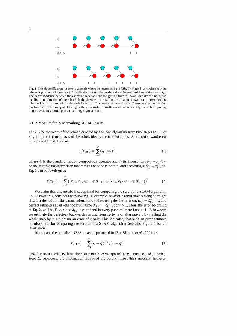
Fig. 1 This figure illustrates a simple example where the metric in Eq. 1fails. The light blue circles show thereference positions of the robotx∗i while the dark red circles show the estimated positions of therobotxi.The correspondence between the estimated locations and the ground truth is shown with dashed lines, andthe direction of motion of the robot is highlighted with arrows. In the situation shown in the upper part, therobot makes a small mistake at the end of the path. This results ina small error. Conversely, in the situationillustrated on the bottom part of the figure the robot makes a small error of the same entity, but at the beginningof the travel, thus resulting in a much bigger global error.

3.1 A Measure for Benchmarking SLAM Results

Let x1:T be the poses of the robot estimated by a SLAM algorithm from time step 1 toT. Letx∗1:T be the reference poses of the robot, ideally the true locations. A straightforward errormetric could be defined as

ε(x1:T) =T

∑t=1

(xt ⊖x∗t )2, (1)

where⊕ is the standard motion composition operator and⊖ its inverse. Letδi, j = x j ⊖ xi

be the relative transformation that moves the nodexi ontox j and accordinglyδ ∗i, j = x∗j ⊖x∗i .

Eq. 1 can be rewritten as

ε(x1:T) =T

∑t=1

(

(x1⊕δ1,2⊕ . . .⊕δt−1,t)⊖ (x∗1⊕δ ∗1,2⊕ . . .⊕δ ∗

t−1,t))2

(2)

We claim that this metric is suboptimal for comparing the result of a SLAM algorithm.To illustrate this, consider the following 1D example in which a robot travels along a straightline. Let the robot make a translational error ofeduring the first motion,δ1,2 = δ ∗

1,2 +e, andperfect estimates at all other points in timeδt,t+1 = δ ∗

t,t+1 for t > 1. Thus, the error accordingto Eq. 2, will beT ·e, sinceδ1,2 is contained in every pose estimate fort > 1. If, however,we estimate the trajectory backwards starting fromxT to x1 or alternatively by shifting thewhole map bye, we obtain an error ofe only. This indicates, that such an error estimateis suboptimal for comparing the results of a SLAM algorithm.See also Figure 1 for anillustration.

In the past, the so-called NEES measure proposed in[Bar-Shalomet al., 2001] as

ε(x1:T) =T

∑t=1

(xt −x∗t )TΩt(xt −x∗t ), (3)

has often been used to evaluate the results of a SLAM approach(e.g.,[Eusticeet al., 2005b]).Here Ωt represents the information matrix of the posext . The NEES measure, however,

7

suffers from a similar problem as Eq. 1 when computingε. In addition to that, not all SLAMalgorithms provide an estimate of the information matrix and thus cannot be compared basedon Eq. 3.

Based on this experience, we propose a measure that considers the deformation energythat is needed to transfer the estimate into the ground truth. This can be done — similarto the ideas of the graph mapping introduced by Lu and Milios[1997] — by consideringthe nodes as masses and connections between them as springs.Thus, our metric is based onthe relativedisplacement between robot poses. Instead of comparingx to x∗ (in the globalreference frame), we do the operation based onδ andδ ∗ as

ε(δ ) =1N ∑

i, jtrans(δi, j ⊖δ ∗

i, j)2 + rot(δi, j ⊖δ ∗

i, j)2, (4)

whereN is the number of relative relations andtrans(·) and rot(·) are used to separateand weight the translational and rotational components. Wesuggest that both quantitiesbe evaluated individually. In this case, the error (or transformation energy) in the above-mentioned example will be consistently estimated as the single rotational error no matterwhere the error occurs in the space or in which order the data is processed.

Our error metric, however, leaves open which relative displacementsδi, j are included inthe summation in Eq. 4. Using the metric and selecting relations are two related but differentproblems. Evaluating two approaches based on a different set of relative pose displacementswill obviously result in two different scores. As we will show in the remainder of this section,the setδ and thusδ ∗ can be defined to highlight certain properties of an algorithm.

Note that some researchers prefer the absolute error (absolute value, not squared) insteadof the squared one. We prefer the squared one since it derivesfrom the motivation that themetric measures the energy needed to transform the estimated trajectory into ground truth.However, one can also use the metric using the non-squared error instead of the squared one.In the experimental evaluation, we actually provide both values.

3.2 Selecting Relative Displacements for Evaluation

Benchmarks are designed to compare different algorithms. In the case of SLAM systems,however, the task the robot finally has to solve should define the required accuracy and thisinformation should be considered in the measure.

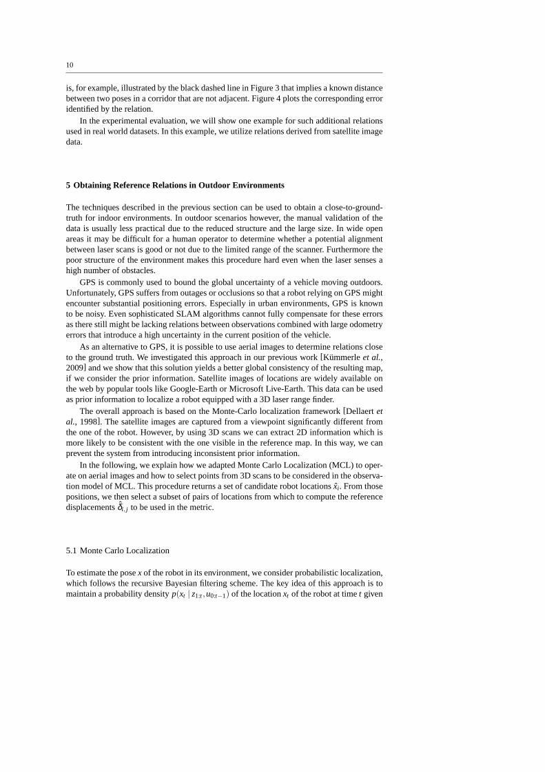
For example, a robot generating blueprints of buildings should reflect the geometry ofa building as accurately as possible. In contrast to that, a robot performing navigation tasksrequires a map that can be used to robustly localize itself and to compute valid trajectoriesto a goal location. To carry out this task, it is sufficient in most cases that the map is topolog-ically consistent and that its observations can be locally matched to the map, i.e. its spatialstructure is correctly representing the environment. We refer to a map having this propertyas being locally consistent. Figure 3 illustrates the concept of locally consistent maps whichare suited for a robot to carry out navigation tasks.

By selecting the relative displacementsδi, j used in Eq. 4 for a given dataset, the user canhighlight certain properties and thus design a measure for evaluating an approach given theapplication in mind.

For example, by adding only known relative displacements between nearby poses basedon visibility, a local consistency is highlighted. In contrast to that, by adding known rela-tive displacements of far away poses, for example, providedby an accurate external mea-surement device or by background knowledge, the accuracy ofthe overall geometry of the

8

mapped environment is enforced. In this way, one can incorporate additional knowledge (forexample, that a corridor has a certain length and is straight) into the benchmark.

4 Obtaining Reference Relations in Indoor Environments

In practice, the key question regarding Eq. 4 is how to determine thetrue relative displace-mentsbetween poses. Obviously, the true values are not available. However, we can de-termine close-to-true values by using the information recorded by the mobile robot andthe background knowledge of the human recording the datasets, which, of course, involvesmanual work.

Please note, that the metric presented above is independentof the actual sensor used. Inthe remainder of this paper, however, we will concentrate onrobots equipped with a laserrange finders, since they are probably the most popular sensors in robotics at the moment.Toevaluate an approach operating on a different sensor modality, one has two possibilities togenerate relations. One way would be to temporarily mount a laser range finder on the robotand calibrate it in the robot coordinate frame. If this is notpossible, one has to providea method for accurately determining the relative displacements between two poses fromwhich an observation has been taken that observes the same part of the space.

4.1 Initial Guess

In our work, we propose the following strategy. First, one tries to find an initial guess aboutthe relative displacement between poses. Based on the knowledge of the human, a wrong ini-tial guess can be easily discarded since the human “knows” the structure of the environment.In a second step, a refinement is proposed based on manual interaction.

4.1.1 Symeo System

One way for obtaining good initial guesses with no or only very few interactions can bethe use of the Symeo Positioning System LPR-B[Symeo GmbH, 2008]. It works similar toa local GPS system but indoors and can achieve a localizationaccuracy of around 5 cm to10 cm. The problem is that such a system designed for industrial applications is typicallynot present at most robotics labs. If available, however, itis well suited for a rather accurateinitial guess of the robot’s position.

4.1.2 Initial Estimate via SLAM Approaches

In most cases, however, researchers in robotics will have SLAM algorithms at hand that canbe used to compute an initial guess about the poses of the robot. In the recent years, severalaccurate methods have been proposed to serve as such a guess (see Section 2). By manuallyinspecting the estimates of the algorithm, a human can accept, refine, or discard a match andalso add missing relations.

It is important to note that the output is not more than an initial guess and it is used toestimate the visibility constraints which will be used in the next step.

9

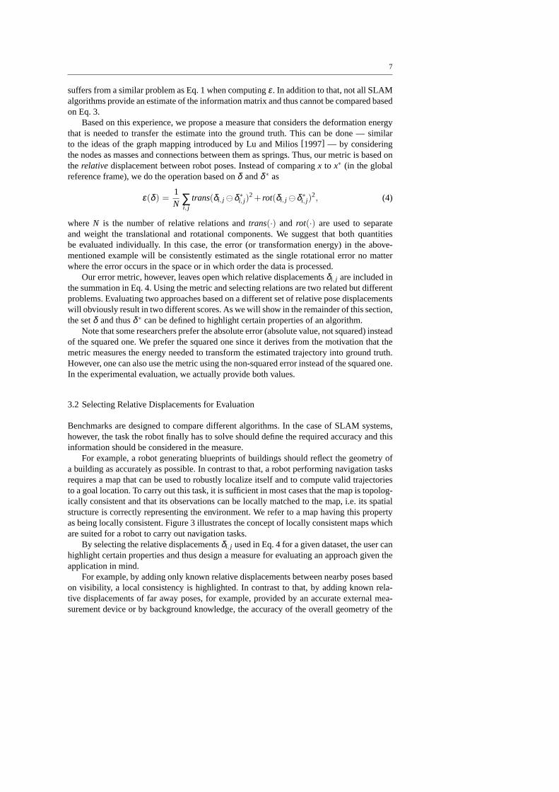
Fig. 2 User interface for matching, accepting, and discarding pairs of observations.

4.2 Manual Matching Refinement and Rejection

Based on the initial guess about the position of the robot fora given time step, it is possibleto determine which observations in the dataset should have covered the same part of thespace or the same objects. For a laser range finder, this can easily be achieved. Betweeneach visible pair of poses, one adds a relative displacementinto a candidate set.

In the next step, a human processes the candidate set to eliminate wrong hypotheses byvisualizing the observation in a common reference frame. This requires manual interactionbut allows for eliminating wrong matches and outliers with high precision, since the user isable to incorporate his background knowledge about the environment.

Since we aim to find the best possible relative displacement,we perform a pair-wiseregistration procedure to refine the estimates of the observation registration method. It fur-thermore allows the user to manually adjust the relative offset between poses so that thepairs of observations fit better. Alternatively, the pair can be discarded.

This approach might sound labor-intensive but with an appropriate user interface, thistask can be carried out without a large waste of resources. For example, for a standard datasetwith 1,700 relations, it took an unexperienced user approximately four hours to extract therelative translations that then served as the input to the error calculation. Figure 2 shows ascreen-shot of the user interface used for evaluation.

It should be noted that for the manual work described above some kind of structure inthe environment is required. The manual labor might be very hard in highly unstructuredscenes.

4.3 Other Relations

In addition to the relative transformations added upon visibility and matching of observa-tions, one can directly incorporate additional relations resulting from other sources of infor-mation, for example, given the knowledge about the length ofa corridor in an environment.By adding a relation between two poses — each at one side of thecorridor — one can incor-porate knowledge about the global geometry of an environment if this is available. This fact

10

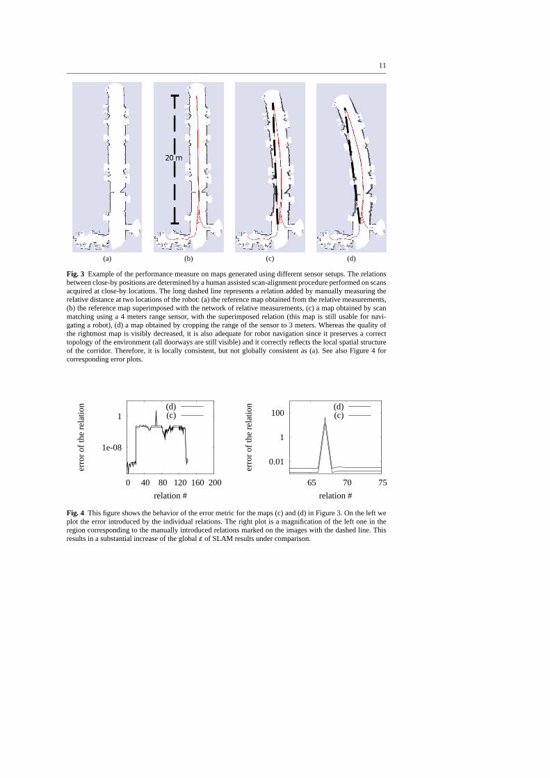
is, for example, illustrated by the black dashed line in Figure 3 that implies a known distancebetween two poses in a corridor that are not adjacent. Figure4 plots the corresponding erroridentified by the relation.

In the experimental evaluation, we will show one example forsuch additional relationsused in real world datasets. In this example, we utilize relations derived from satellite imagedata.

5 Obtaining Reference Relations in Outdoor Environments

The techniques described in the previous section can be usedto obtain a close-to-ground-truth for indoor environments. In outdoor scenarios however, the manual validation of thedata is usually less practical due to the reduced structure and the large size. In wide openareas it may be difficult for a human operator to determine whether a potential alignmentbetween laser scans is good or not due to the limited range of the scanner. Furthermore thepoor structure of the environment makes this procedure hardeven when the laser senses ahigh number of obstacles.

GPS is commonly used to bound the global uncertainty of a vehicle moving outdoors.Unfortunately, GPS suffers from outages or occlusions so that a robot relying on GPS mightencounter substantial positioning errors. Especially in urban environments, GPS is knownto be noisy. Even sophisticated SLAM algorithms cannot fully compensate for these errorsas there still might be lacking relations between observations combined with large odometryerrors that introduce a high uncertainty in the current position of the vehicle.

As an alternative to GPS, it is possible to use aerial images to determine relations closeto the ground truth. We investigated this approach in our previous work[Kummerleet al.,2009] and we show that this solution yields a better global consistency of the resulting map,if we consider the prior information. Satellite images of locations are widely available onthe web by popular tools like Google-Earth or Microsoft Live-Earth. This data can be usedas prior information to localize a robot equipped with a 3D laser range finder.

The overall approach is based on the Monte-Carlo localization framework[Dellaertetal., 1998]. The satellite images are captured from a viewpoint significantly different fromthe one of the robot. However, by using 3D scans we can extract2D information which ismore likely to be consistent with the one visible in the reference map. In this way, we canprevent the system from introducing inconsistent prior information.

In the following, we explain how we adapted Monte Carlo Localization (MCL) to oper-ate on aerial images and how to select points from 3D scans to be considered in the observa-tion model of MCL. This procedure returns a set of candidate robot locations ˆxi . From thosepositions, we then select a subset of pairs of locations fromwhich to compute the referencedisplacementsδi, j to be used in the metric.

5.1 Monte Carlo Localization

To estimate the posex of the robot in its environment, we consider probabilistic localization,which follows the recursive Bayesian filtering scheme. The key idea of this approach is tomaintain a probability densityp(xt | z1:t ,u0:t−1) of the locationxt of the robot at timet given

11

(a) (b) (c) (d)

Fig. 3 Example of the performance measure on maps generated using different sensor setups. The relationsbetween close-by positions are determined by a human assistedscan-alignment procedure performed on scansacquired at close-by locations. The long dashed line represents a relation added by manually measuring therelative distance at two locations of the robot: (a) the reference map obtained from the relative measurements,(b) the reference map superimposed with the network of relative measurements, (c) a map obtained by scanmatching using a 4 meters range sensor, with the superimposed relation (this map is still usable for navi-gating a robot), (d) a map obtained by cropping the range of thesensor to 3 meters. Whereas the quality ofthe rightmost map is visibly decreased, it is also adequate forrobot navigation since it preserves a correcttopology of the environment (all doorways are still visible)and it correctly reflects the local spatial structureof the corridor. Therefore, it is locally consistent, but not globally consistent as (a). See also Figure 4 forcorresponding error plots.

1e-08

1

0 40 80 120 160 200

erro

r of

the

rela

tion

relation #

(d)(c)

0.01

1

100

65 70 75

erro

r of

the

rela

tion

relation #

(d)(c)

Fig. 4 This figure shows the behavior of the error metric for the maps (c) and (d) in Figure 3. On the left weplot the error introduced by the individual relations. The right plot is a magnification of the left one in theregion corresponding to the manually introduced relations marked on the images with the dashed line. Thisresults in a substantial increase of the globalε of SLAM results under comparison.

12

(a) (b)

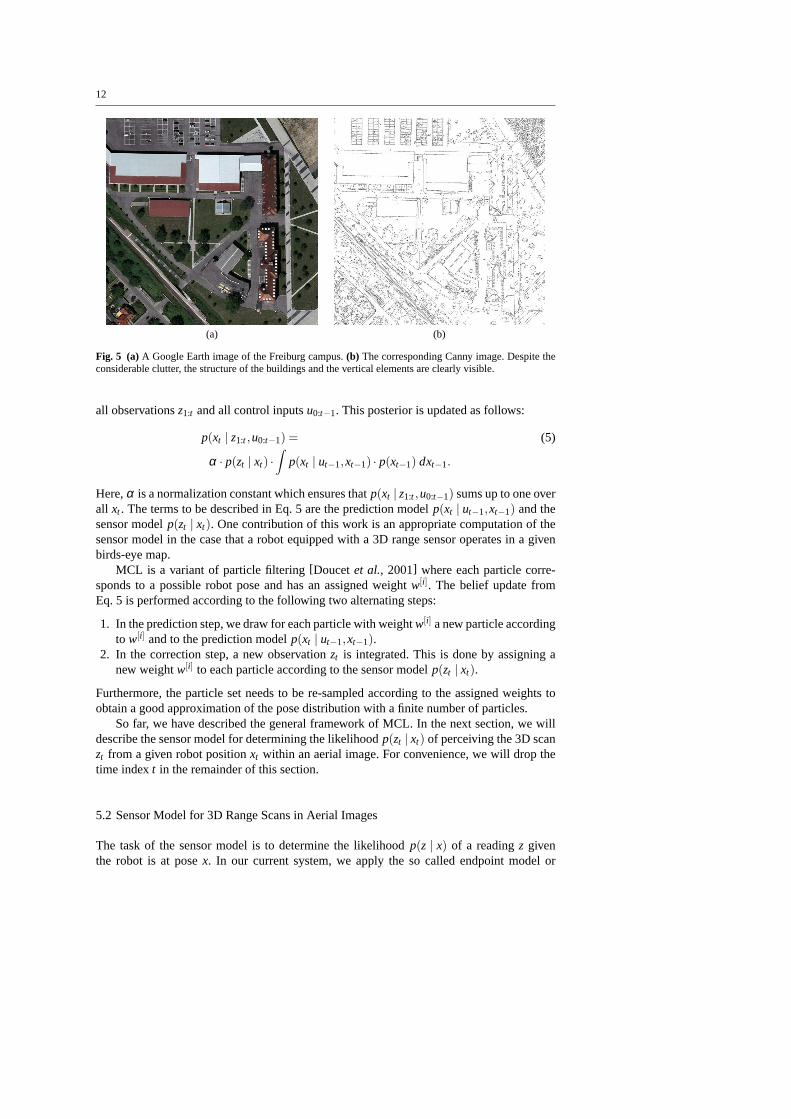
Fig. 5 (a)A Google Earth image of the Freiburg campus.(b) The corresponding Canny image. Despite theconsiderable clutter, the structure of the buildings and the vertical elements are clearly visible.

all observationsz1:t and all control inputsu0:t−1. This posterior is updated as follows:

p(xt | z1:t ,u0:t−1) = (5)

α · p(zt | xt) ·∫

p(xt | ut−1,xt−1) · p(xt−1) dxt−1.

Here,α is a normalization constant which ensures thatp(xt | z1:t ,u0:t−1) sums up to one overall xt . The terms to be described in Eq. 5 are the prediction modelp(xt | ut−1,xt−1) and thesensor modelp(zt | xt). One contribution of this work is an appropriate computation of thesensor model in the case that a robot equipped with a 3D range sensor operates in a givenbirds-eye map.

MCL is a variant of particle filtering[Doucetet al., 2001] where each particle corre-sponds to a possible robot pose and has an assigned weightw[i]. The belief update fromEq. 5 is performed according to the following two alternating steps:

1. In the prediction step, we draw for each particle with weight w[i] a new particle accordingto w[i] and to the prediction modelp(xt | ut−1,xt−1).

2. In the correction step, a new observationzt is integrated. This is done by assigning anew weightw[i] to each particle according to the sensor modelp(zt | xt).

Furthermore, the particle set needs to be re-sampled according to the assigned weights toobtain a good approximation of the pose distribution with a finite number of particles.

So far, we have described the general framework of MCL. In thenext section, we willdescribe the sensor model for determining the likelihoodp(zt | xt) of perceiving the 3D scanzt from a given robot positionxt within an aerial image. For convenience, we will drop thetime indext in the remainder of this section.

5.2 Sensor Model for 3D Range Scans in Aerial Images

The task of the sensor model is to determine the likelihoodp(z | x) of a readingz giventhe robot is at posex. In our current system, we apply the so called endpoint modelor

13

likelihood fields[Thrunet al., 2005]. Let zk be the endpoints of a 3D scanz. The endpointmodel computes the likelihood of a reading based only on the distances between a scan pointzk re-projected onto the map according to the posex of the robot and the point in the mapdk

which is closest to ˆzk as:

p(z | x) = f (‖z1− d1‖, . . . ,‖zk− dk‖). (6)

If we assume that the beams are independent and the sensor noise is normally distributed wecan rewrite Eq. 6 as

f (‖z1− d1‖, . . . ,‖zk− dk‖) ∝ ∏j

e(zj−d j )2

σ2 . (7)

Since the aerial image only contains 2D information about the scene, we need to select aset of beams from the 3D scan, which are likely to result in structures that can be identifiedand matched in the image. In other words, we need to transformboth the scan and the imageinto a set of 2D points which can be compared via the functionf (·).

To extract these points from the image we employ the standardCanny edge extractionprocedure[Canny, 1986]. The idea behind this is that if there is a height gap in the aerialimage, there will often also be a visible change in intensityin the aerial image and weassume that this intensity change is detected by the edge extraction procedure. In an urbanenvironment, such edges typically correspond to borders ofroofs, trees, fences or otherstructures. Of course, the edge extraction procedure returns a lot of false positives that donot represent any actual 3D structure, like street markings, grass borders, shadows, and otherflat markings. All these aspects have to be considered by the sensor model.

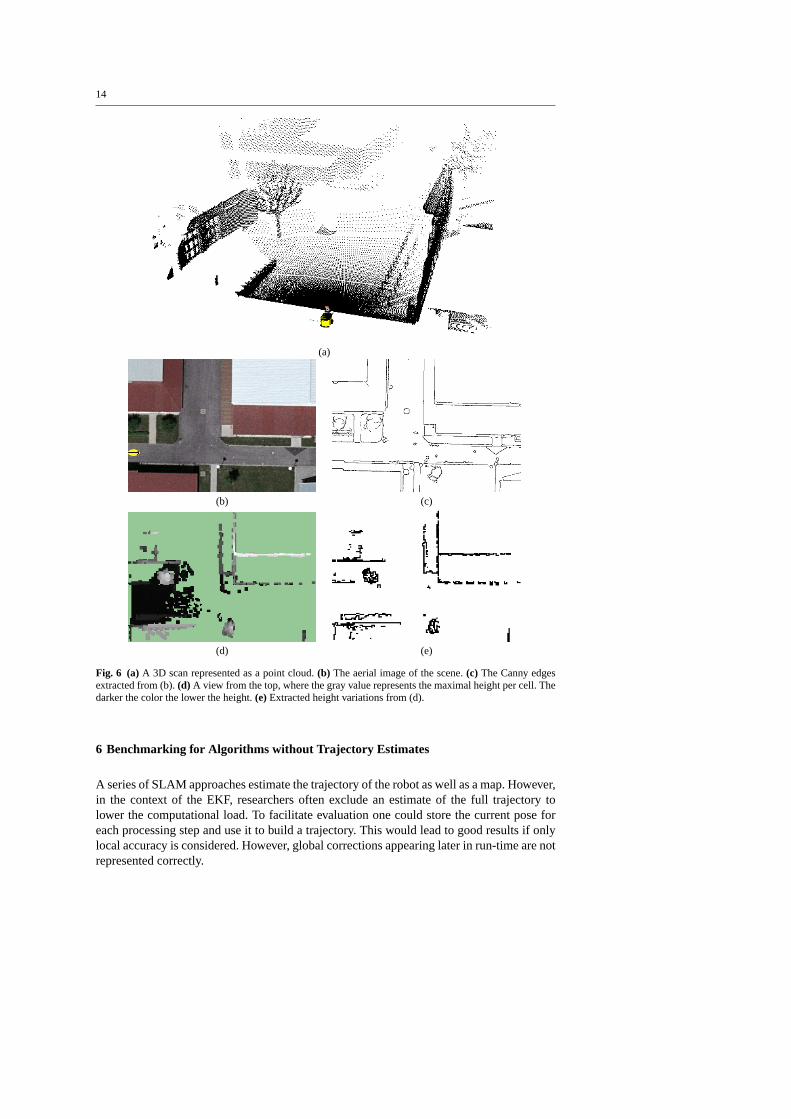
A straightforward way to address this problem is to select a subset of beamszk fromthe 3D scan which will then be used to compute the likelihood.The beams which shouldbe considered are the ones which correspond to significant variations along thez directionof the 3D scan. For vertical structures, a direct matching between the extracted edges andthe measurements of a horizontal 2D laser range scanner can be performed, as discussed byFruh and Zakhor[2004]. If a 3D laser range finder is available, we also attempt to matchvariations in height that are not purely vertical structures, like trees or overhanging roofs.This procedure is illustrated by the sequence of images in Figure 6.

In the current implementation, we considered variations inheight of 0.5 m and aboveas possible positions of edges that could also be visible in the aerial image. The positionsof these variations relative to the robot can then be matchedagainst the Canny edges of theaerial image in a point-by-point fashion, similar to the matching of 2D-laser scans againstan occupancy grid map. Additionally, we employ a heuristic to detect when the prior is notavailable, i.e., when the robot is inside of a building or under overhanging structures. This isbased on the 3D perception. If there is a ceiling which leads to range measurements abovethe robot no global relations from the localization are integrated, since we assume that thearea the robot is sensing is not visible in the aerial image.

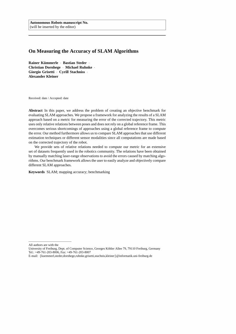
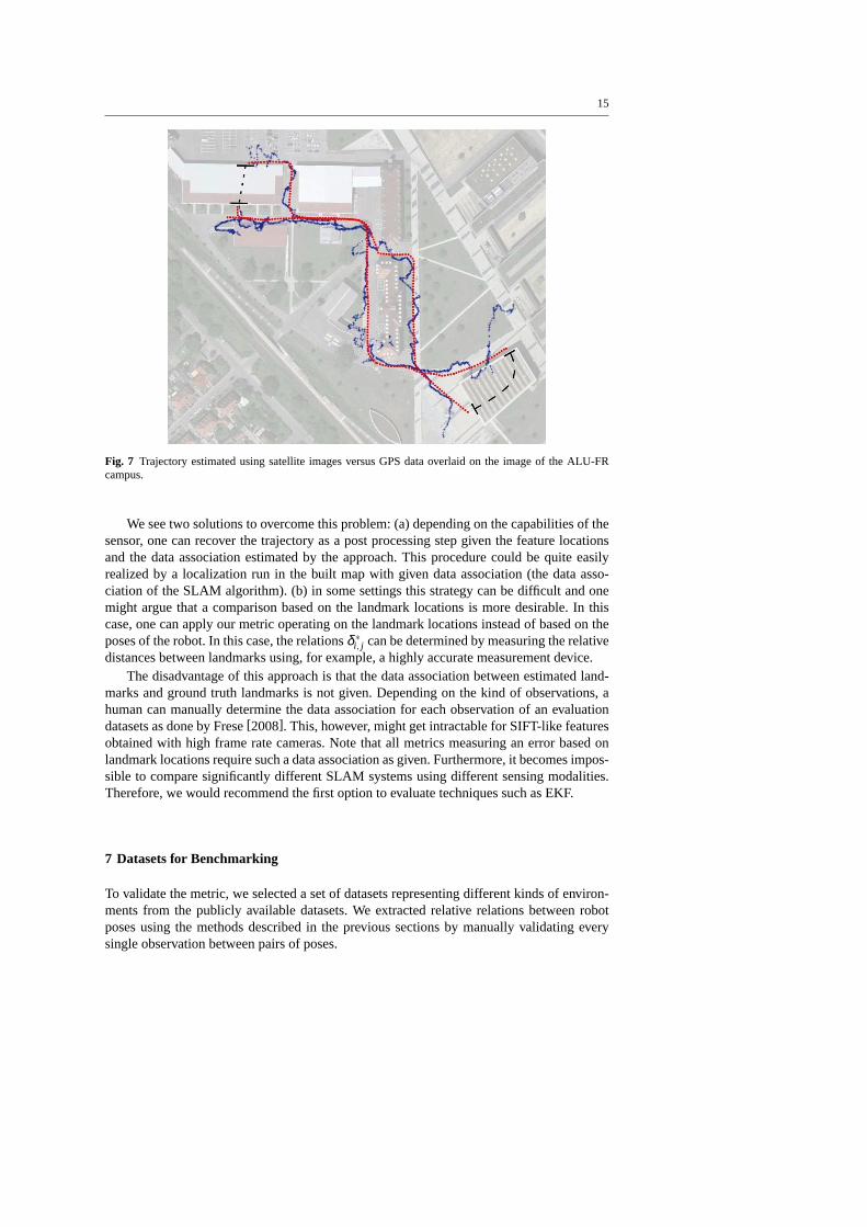
Figure 7 shows an example trajectory estimated with this technique (in red) and theGPS positions (in blue). As can be seen, the estimates are more accurate than the GPSdata. Thus the improved guess facilitates the manual verification of the data. Note that theapproach presented here is used to obtain the candidate relations for outdoor datasets. Ahuman operator has to accept or decline all relations found by the approach.

14

(a)

(b) (c)

(d) (e)

Fig. 6 (a) A 3D scan represented as a point cloud.(b) The aerial image of the scene.(c) The Canny edgesextracted from (b).(d) A view from the top, where the gray value represents the maximalheight per cell. Thedarker the color the lower the height.(e)Extracted height variations from (d).

6 Benchmarking for Algorithms without Trajectory Estimates

A series of SLAM approaches estimate the trajectory of the robot as well as a map. However,in the context of the EKF, researchers often exclude an estimate of the full trajectory tolower the computational load. To facilitate evaluation onecould store the current pose foreach processing step and use it to build a trajectory. This would lead to good results if onlylocal accuracy is considered. However, global correctionsappearing later in run-time are notrepresented correctly.

15

Fig. 7 Trajectory estimated using satellite images versus GPS data overlaid on the image of the ALU-FRcampus.

We see two solutions to overcome this problem: (a) dependingon the capabilities of thesensor, one can recover the trajectory as a post processing step given the feature locationsand the data association estimated by the approach. This procedure could be quite easilyrealized by a localization run in the built map with given data association (the data asso-ciation of the SLAM algorithm). (b) in some settings this strategy can be difficult and onemight argue that a comparison based on the landmark locations is more desirable. In thiscase, one can apply our metric operating on the landmark locations instead of based on theposes of the robot. In this case, the relationsδ ∗

i, j can be determined by measuring the relativedistances between landmarks using, for example, a highly accurate measurement device.

The disadvantage of this approach is that the data association between estimated land-marks and ground truth landmarks is not given. Depending on the kind of observations, ahuman can manually determine the data association for each observation of an evaluationdatasets as done by Frese[2008]. This, however, might get intractable for SIFT-like featuresobtained with high frame rate cameras. Note that all metricsmeasuring an error based onlandmark locations require such a data association as given. Furthermore, it becomes impos-sible to compare significantly different SLAM systems usingdifferent sensing modalities.Therefore, we would recommend the first option to evaluate techniques such as EKF.

7 Datasets for Benchmarking

To validate the metric, we selected a set of datasets representing different kinds of environ-ments from the publicly available datasets. We extracted relative relations between robotposes using the methods described in the previous sections by manually validating everysingle observation between pairs of poses.

16

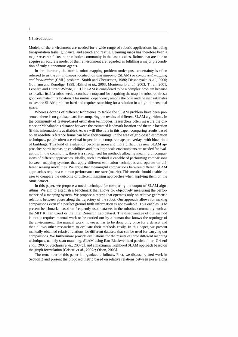
Fig. 8 Maps obtained by the reference datasets used to validate ourmetric. From top to bottom and left toright: MIT Killian Court (Boston), ACES Building (Austin),Intel Research Lab (Seattle), MIT CS Building(Boston), building 079 University of Freiburg, and the University Hospital in Freiburg. The depicted mapof the University Hospital was obtained by using the background information extracted from the satelliteimages.

17

As a challenging indoor corridor-environment with a non-trivial topology includingnested loops, we selected the MIT Killian Court dataset1 (Infinite Corridor) and the datasetof the ACES building at the University of Texas, Austin2. As a typical office environmentwith a significant level of clutter, we selected the dataset of building 079 at the Univer-sity of Freiburg, the Intel Research Lab dataset3, and a dataset acquired at the CSAIL atMIT. For addressing outdoor environments, we recorded a newdataset at the park area ofthe University Hospital, Freiburg. To give a visual impression of the scanned environments,Figure 8 illustrates maps obtained by executing state-of-the-art SLAM algorithms[Grisettiet al., 2007b; 2007c; Olson, 2008]. All datasets, the manually verified relations, and mapimages are available online at:http://ais.informatik.uni-freiburg.de/slamevaluation/

8 Experimental Evaluation

This evaluation is designed to illustrate the properties ofour method. We selected three pop-ular mapping techniques, namely scan matching, a Rao-Blackwellized particle filter-basedapproach, and a graph-based solution to the SLAM problem andprocessed the datasets dis-cussed in the previous section.

We provide the scores obtained from the metric for all combinations of SLAM approachand dataset. This will allow other researchers to compare their own SLAM approachesagainst our methods using the provided benchmark datasets.In addition, we also presentsub-optimally corrected trajectories in this section to illustrate how inconsistencies affectthe score of the metric. We will show that our error metric is well-suited for benchmarkingand this kind of evaluation.

8.1 Evaluation of Existing Approaches using the Proposed Metric

In this evaluation, we considered the following mapping approaches:

Scan Matching: Scan matching is the computation of the incremental, open loop maxi-mum likelihood trajectory of the robot by matching consecutive scans[Lu and Milios,1994; Censi, 2006]. In small environments, a scan matching algorithm is generally suf-ficient to obtain accurate maps with a comparably small computational effort. However,the estimate of the robot trajectory computed by scan matching is affected by an in-creasing error which becomes visible whenever the robot reenters in known regionsafter visiting large unknown areas (loop closing or place revisiting).

Grid-based Rao-Blackwellized Particle Filter (RBPF) for SLAM: We use the RBPFimplementation described in[Grisetti et al., 2007b; Stachnisset al., 2007b] which isavailable online[Stachnisset al., 2007a]. It estimates the posterior over maps and tra-jectories by means of a particle filter. Each particle carries its own map and a hypothesisof the robot pose within that map. The approach uses an informed proposal distributionfor particle generation that is optimized to laser range data. In the evaluation presentedhere, we used 50 particles. Note that a higher number of samples may improve the per-formance of the algorithm.

1 Courtesy of Mike Bosse2 Courtesy of Patrick Beeson3 Courtesy of Dirk Haehnel

18

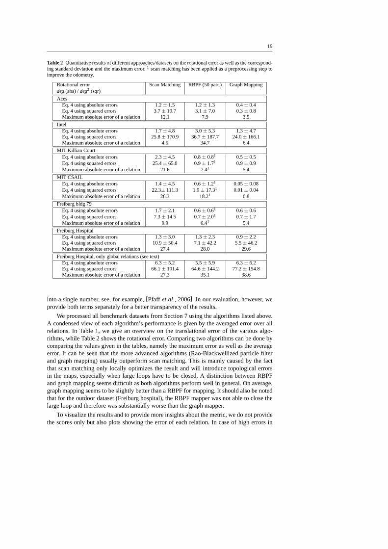
Table 1 Quantitative results of different approaches/datasets onthe translation error as well as the corre-sponding standard deviation and the maximum error.1 scan matching has been applied as a preprocessingstep to improve the odometry.

Translational error Scan Matching RBPF (50 part.) Graph Mappingm (abs) /m2 (sqr)

AcesEq. 4 using absolute errors 0.173± 0.614 0.060± 0.049 0.044± 0.044Eq. 4 using squared errors 0.407± 2.726 0.006± 0.011 0.004± 0.009Maximum absolute error of a relation 4.869 0.433 0.347

IntelEq. 4 using absolute errors 0.220± 0.296 0.070± 0.083 0.031± 0.026Eq. 4 using squared errors 0.136± 0.277 0.011± 0.034 0.002± 0.004Maximum absolute error of a relation 1.168 0.698 0.229

MIT Killian CourtEq. 4 using absolute errors 1.651± 4.138 0.122± 0.3861 0.050± 0.056Eq. 4 using squared errors 19.85± 59.84 0.164± 0.8141 0.006± 0.029Maximum absolute error of a relation 19.467 2.5131 0.765

MIT CSAILEq. 4 using absolute errors 0.106± 0.325 0.049± 0.0491 0.004± 0.009Eq. 4 using squared errors 0.117± 0.728 0.005± 0.0131 0.0001± 0.0005Maximum absolute error of a relation 3.570 0.5081 0.096

Freiburg bldg 79Eq. 4 using absolute errors 0.258± 0.427 0.061± 0.0441 0.056± 0.042Eq. 4 using squared errors 0.249± 0.687 0.006± 0.0201 0.005± 0.011Maximum absolute error of a relation 2.280 0.8561 0.459

Freiburg HospitalEq. 4 using absolute errors 0.434± 1.615 0.637± 2.638 0.143± 0.180Eq. 4 using squared errors 2.79± 18.19 7.367± 38.496 0.053± 0.272Maximum absolute error of a relation 15.584 15.343 2.385

Freiburg Hospital, only global relations (see text)Eq. 4 using absolute errors 13.0± 11.6 12.3± 11.7 11.6± 11.9Eq. 4 using squared errors 305.4± 518.9 288.8± 626.3 276.1± 516.5Maximum absolute error of a relation 70.9 65.1 66.1

Graph Mapping: This approach computes a map by means of graph optimization[Grisettiet al., 2007c]. The idea is to construct a graph out of the sequence of measurements. Ev-ery node in the graph represents a pose along the trajectory taken by the robot and thecorresponding measurement obtained at that pose. Then, a least square error minimiza-tion approach is applied to obtain the most-likely configuration of the graph. In general,it is non-trivial to find the constraints, often referred to as the data association problem.Especially in symmetric environments or in situations withlarge noise, the edges in thegraph may be wrong or imprecise and thus the resulting map mayyields inconsistencies.In our current implementation of the graph mapping system, we followed the approachof Olson[2008] to compute constraints.

For our evaluation, we manually extracted the relations forall datasets mentioned in theprevious section. The manually extracted relations are available online, see Section 7. Wethen carried out the mapping approaches and used the corrected trajectory for computing theerror according to our metric. Please note, that the error computed according to our metric(as well as for most other metrics too) can be separated into two components: a translationalerror and a rotational error. Often, a “weighting-factor” is used to combine both error terms

19

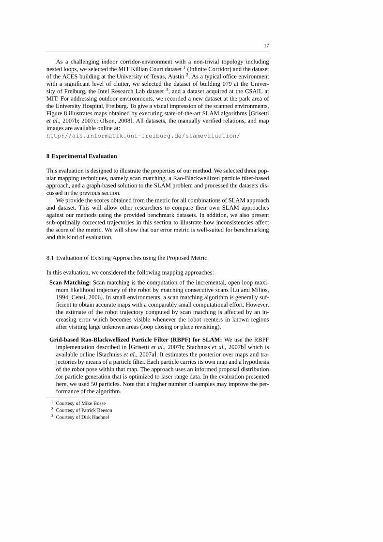
Table 2 Quantitative results of different approaches/datasets onthe rotational error as well as the correspond-ing standard deviation and the maximum error.1 scan matching has been applied as a preprocessing step toimprove the odometry.

Rotational error Scan Matching RBPF (50 part.) Graph Mappingdeg(abs) /deg2 (sqr)

AcesEq. 4 using absolute errors 1.2± 1.5 1.2± 1.3 0.4± 0.4Eq. 4 using squared errors 3.7± 10.7 3.1± 7.0 0.3± 0.8Maximum absolute error of a relation 12.1 7.9 3.5

IntelEq. 4 using absolute errors 1.7± 4.8 3.0± 5.3 1.3± 4.7Eq. 4 using squared errors 25.8± 170.9 36.7± 187.7 24.0± 166.1Maximum absolute error of a relation 4.5 34.7 6.4

MIT Killian CourtEq. 4 using absolute errors 2.3± 4.5 0.8± 0.81 0.5± 0.5Eq. 4 using squared errors 25.4± 65.0 0.9± 1.71 0.9± 0.9Maximum absolute error of a relation 21.6 7.41 5.4

MIT CSAILEq. 4 using absolute errors 1.4± 4.5 0.6± 1.21 0.05± 0.08Eq. 4 using squared errors 22.3± 111.3 1.9± 17.31 0.01± 0.04Maximum absolute error of a relation 26.3 18.21 0.8

Freiburg bldg 79Eq. 4 using absolute errors 1.7± 2.1 0.6± 0.61 0.6± 0.6Eq. 4 using squared errors 7.3± 14.5 0.7± 2.01 0.7± 1.7Maximum absolute error of a relation 9.9 6.41 5.4

Freiburg HospitalEq. 4 using absolute errors 1.3± 3.0 1.3± 2.3 0.9± 2.2Eq. 4 using squared errors 10.9± 50.4 7.1± 42.2 5.5± 46.2Maximum absolute error of a relation 27.4 28.0 29.6

Freiburg Hospital, only global relations (see text)Eq. 4 using absolute errors 6.3± 5.2 5.5± 5.9 6.3± 6.2Eq. 4 using squared errors 66.1± 101.4 64.6± 144.2 77.2± 154.8Maximum absolute error of a relation 27.3 35.1 38.6

into a single number, see, for example,[Pfaff et al., 2006]. In our evaluation, however, weprovide both terms separately for a better transparency of the results.

We processed all benchmark datasets from Section 7 using thealgorithms listed above.A condensed view of each algorithm’s performance is given bythe averaged error over allrelations. In Table 1, we give an overview on the translational error of the various algo-rithms, while Table 2 shows the rotational error. Comparingtwo algorithms can be done bycomparing the values given in the tables, namely the maximumerror as well as the averageerror. It can be seen that the more advanced algorithms (Rao-Blackwellized particle filterand graph mapping) usually outperform scan matching. This is mainly caused by the factthat scan matching only locally optimizes the result and will introduce topological errorsin the maps, especially when large loops have to be closed. A distinction between RBPFand graph mapping seems difficult as both algorithms performwell in general. On average,graph mapping seems to be slightly better than a RBPF for mapping. It should also be notedthat for the outdoor dataset (Freiburg hospital), the RBPF mapper was not able to close thelarge loop and therefore was substantially worse than the graph mapper.

To visualize the results and to provide more insights about the metric, we do not providethe scores only but also plots showing the error of each relation. In case of high errors in

20

a block of relations, we label the relations in the maps. Thisenables us to see not onlywhere an algorithm fails, but can also provide insights as towhy it fails. Inspecting thosesituations in correlation with the map helps to understand the properties of algorithms andgives valuable insights on its capabilities. For three datasets, a detailed analysis using theseplots is presented in Section 8.2 to Section 8.4. The overallanalysis provides the intuitionthat our metric is well-suited for evaluating SLAM approaches.

8.2 MIT Killian Court

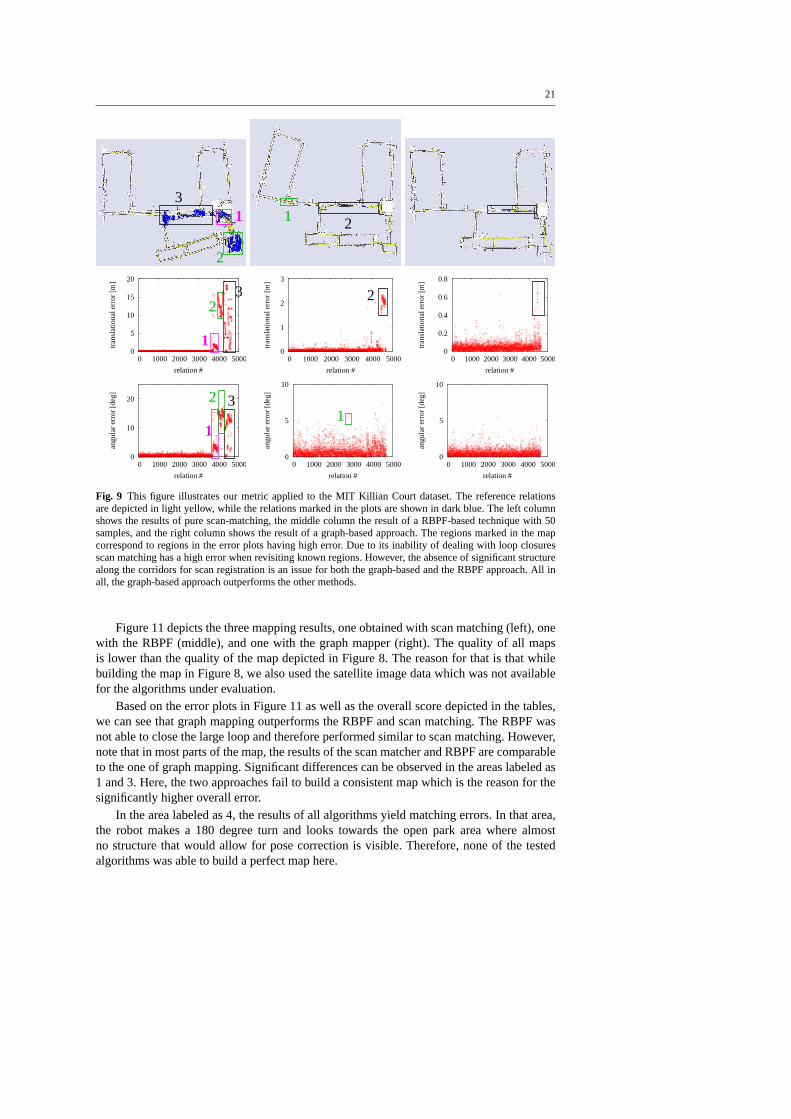
The MIT Killian Court dataset has been acquired in a large indoor environment, wherethe robot mainly observed corridors lacking structures that support accurate pose correc-tion. The robot traverses multiple nested loops – a challenge especially for the RBPF-basedtechnique. We extracted close to 5,000 relations between nearby poses that are used forevaluation. Figure 9 shows three different results and the corresponding error distributionsto illustrate the capabilities of our method. Regions in themap with high inconsistenciescorrespond to relations having a high error. The absence of significant structure along thecorridors results in a small or medium re-localization error of the robot in all compared ap-proaches. In sum, we can say the graph-based approach outperforms the other methods andthat the score of our metric reflects the impression of a humanabout map quality obtained byvisually inspecting the mapping results (the vertical corridors in the upper part are supposedto be parallel).

8.3 Freiburg Indoor Building 079

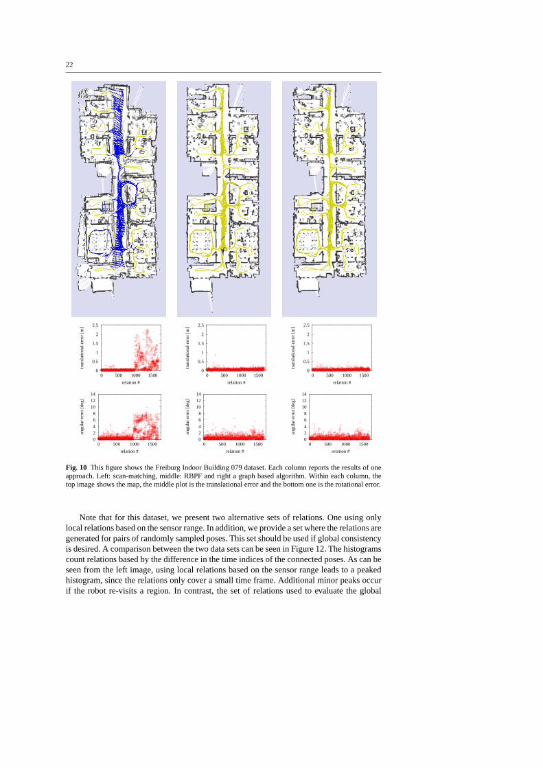
The building 079 of the University of Freiburg is an example for an indoor office environ-ment. The building consists of one corridor which connects the individual rooms. Figure 10depicts the results of the individual algorithms (scan matching, RBPF, graph-based). In thefirst row of Figure 10, the relations having a translational error greater than 0.15 m are high-lighted in blue.

In the left plot showing the scan matching result, the relations plotted in blue are gen-erated when the robot revisits an already known region. These relations are visible in thecorresponding error plots (Figure 10 first column, second and third row). As can be seenfrom the error plots, the relations with a number greater than 1,000 have a larger error thanthe rest of the dataset. The fact that the pose estimate of therobot is sub-optimal and that theerror accumulates can also be seen by the rather blurry map and that some walls occur twice.In contrast to that, the more sophisticated algorithms, namely RBPF and graph mapping, areable to produce consistent and accurate maps in this environment. Only very few relationsshow an increased error (illustrated by dark blue relations).

8.4 Freiburg University Hospital

This dataset consists of 2D and 3D laser range data obtained with one statically mountedSICK scanner and one mounted on a pan-tilt unit. The robot wassteered through a park areathat contains a lot of bushes and which is surrounded by buildings. Most of the time, therobot was steered along a bike lane with cobble stone pavement. The area is around 500 mby 250 m in size.

21

0

10

20

0 1000 2000 3000 4000 5000

angu

lar

erro

r [d

eg]

relation #

0

5

10

15

20

0 1000 2000 3000 4000 5000

tran

slat

iona

l err

or [m

]

relation #

0

1

2

3

0 1000 2000 3000 4000 5000

tran

slat

iona

l err

or [m

]

relation #

0

5

10

0 1000 2000 3000 4000 5000

angu

lar

erro

r [d

eg]

relation #

0

0.2

0.4

0.6

0.8

0 1000 2000 3000 4000 5000

tran

slat

iona

l err

or [m

]

relation #

0

5

10

0 1000 2000 3000 4000 5000

angu

lar

erro

r [d

eg]

relation #

3

2

1

2

1

2 3

1

3

1

2

21

Fig. 9 This figure illustrates our metric applied to the MIT Killian Court dataset. The reference relationsare depicted in light yellow, while the relations marked in the plots are shown in dark blue. The left columnshows the results of pure scan-matching, the middle column the result of a RBPF-based technique with 50samples, and the right column shows the result of a graph-basedapproach. The regions marked in the mapcorrespond to regions in the error plots having high error. Due to its inability of dealing with loop closuresscan matching has a high error when revisiting known regions.However, the absence of significant structurealong the corridors for scan registration is an issue for both the graph-based and the RBPF approach. All inall, the graph-based approach outperforms the other methods.

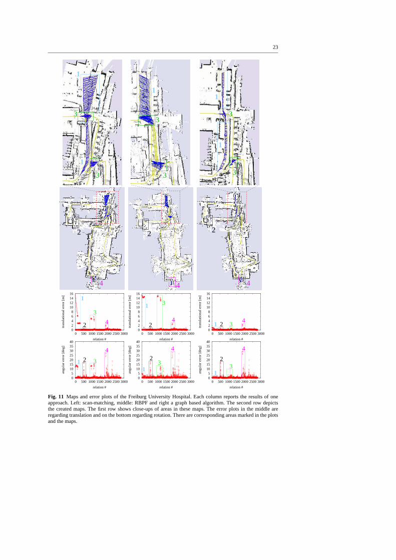
Figure 11 depicts the three mapping results, one obtained with scan matching (left), onewith the RBPF (middle), and one with the graph mapper (right). The quality of all mapsis lower than the quality of the map depicted in Figure 8. The reason for that is that whilebuilding the map in Figure 8, we also used the satellite imagedata which was not availablefor the algorithms under evaluation.

Based on the error plots in Figure 11 as well as the overall score depicted in the tables,we can see that graph mapping outperforms the RBPF and scan matching. The RBPF wasnot able to close the large loop and therefore performed similar to scan matching. However,note that in most parts of the map, the results of the scan matcher and RBPF are comparableto the one of graph mapping. Significant differences can be observed in the areas labeled as1 and 3. Here, the two approaches fail to build a consistent map which is the reason for thesignificantly higher overall error.

In the area labeled as 4, the results of all algorithms yield matching errors. In that area,the robot makes a 180 degree turn and looks towards the open park area where almostno structure that would allow for pose correction is visible. Therefore, none of the testedalgorithms was able to build a perfect map here.

22

0

0.5

1

1.5

2

2.5

0 500 1000 1500

tran

slat

iona

l err

or [m

]

relation #

0

0.5

1

1.5

2

2.5

0 500 1000 1500

tran

slat

iona

l err

or [m

]

relation #

0

0.5

1

1.5

2

2.5

0 500 1000 1500

tran

slat

iona

l err

or [m

]

relation #

0 2 4 6 8

10 12 14

0 500 1000 1500

angu

lar

erro

r [d

eg]

relation #

0 2 4 6 8

10 12 14

0 500 1000 1500

angu

lar

erro

r [d

eg]

relation #

0 2 4 6 8

10 12 14

0 500 1000 1500

angu

lar

erro

r [d

eg]

relation #

Fig. 10 This figure shows the Freiburg Indoor Building 079 dataset. Each column reports the results of oneapproach. Left: scan-matching, middle: RBPF and right a graphbased algorithm. Within each column, thetop image shows the map, the middle plot is the translational error and the bottom one is the rotational error.

Note that for this dataset, we present two alternative sets of relations. One using onlylocal relations based on the sensor range. In addition, we provide a set where the relations aregenerated for pairs of randomly sampled poses. This set should be used if global consistencyis desired. A comparison between the two data sets can be seenin Figure 12. The histogramscount relations based by the difference in the time indices of the connected poses. As can beseen from the left image, using local relations based on the sensor range leads to a peakedhistogram, since the relations only cover a small time frame. Additional minor peaks occurif the robot re-visits a region. In contrast, the set of relations used to evaluate the global

23

0 5

10 15 20 25 30 35 40

0 500 1000 1500 2000 2500 3000

an

gu

lar

err

or

[de

g]

relation #

0 5

10 15 20 25 30 35 40

0 500 1000 1500 2000 2500 3000

an

gu

lar

err

or

[de

g]

relation #

0 5

10 15 20 25 30 35 40

0 500 1000 1500 2000 2500 3000

an

gu

lar

err

or

[de

g]

relation #

0 2 4 6 8

10 12 14 16

0 500 1000 1500 2000 2500 3000

tra

nsl

atio

na

l err

or

[m]

relation #

0 2 4 6 8

10 12 14 16

0 500 1000 1500 2000 2500 3000

tra

nsl

atio

na

l err

or

[m]

relation #

0 2 4 6 8

10 12 14 16

0 500 1000 1500 2000 2500 3000

tra

nsl

atio

na

l err

or

[m]

relation #

4

1

1

3

3

2

1

23

4

3

4

1 2

4

2

1

1

3

3

4

3

2

1

3

3

1

4

2

4321

4

31

2

32

1

4

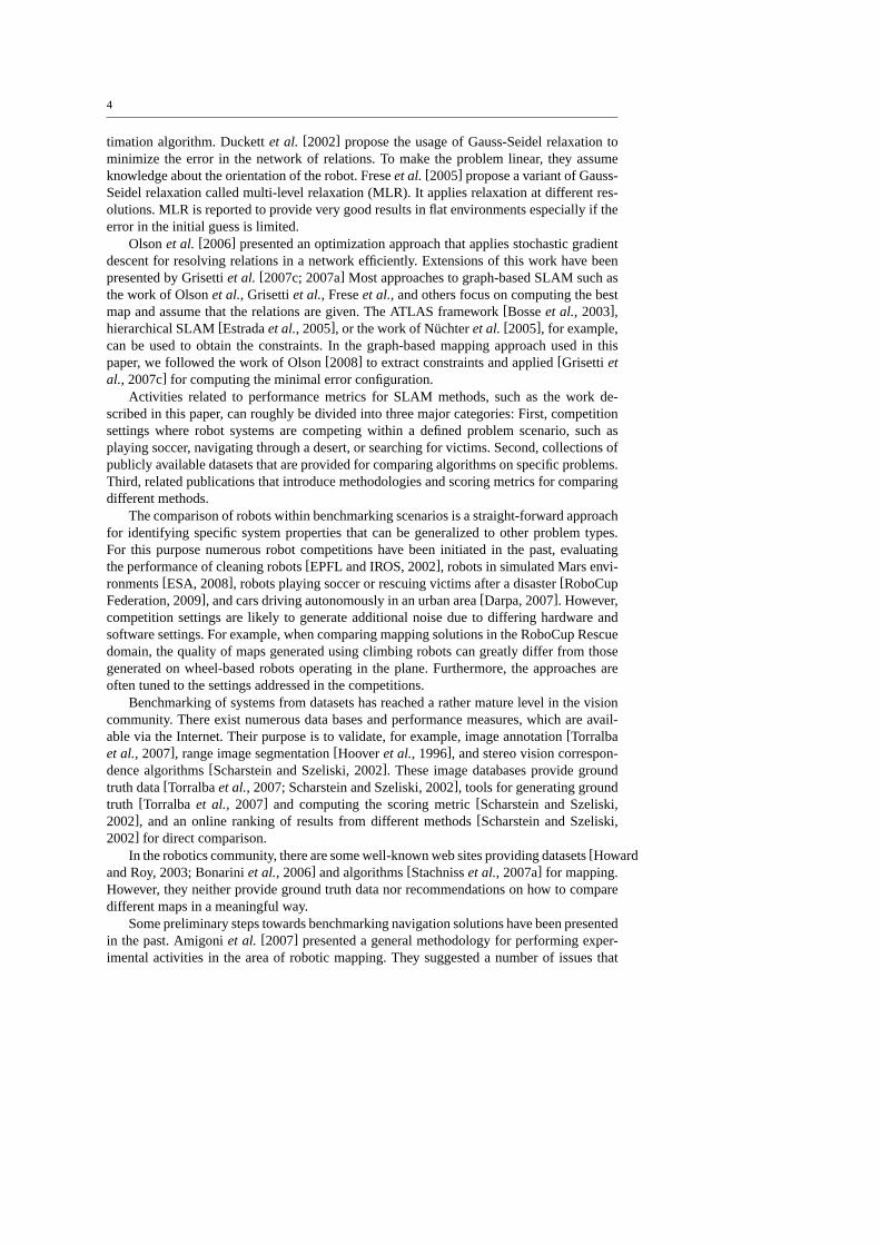
Fig. 11 Maps and error plots of the Freiburg University Hospital. Each column reports the results of oneapproach. Left: scan-matching, middle: RBPF and right a graphbased algorithm. The second row depictsthe created maps. The first row shows close-ups of areas in these maps. The error plots in the middle areregarding translation and on the bottom regarding rotation. There are corresponding areas marked in the plotsand the maps.

24

1

10

100

1000

0 1000 2000 3000 4000 5000 6000 7000

coun

t

# sensor readings between poses

0

1

2

3

4

5

0 1000 2000 3000 4000 5000 6000 7000

coun

t

# sensor readings between poses

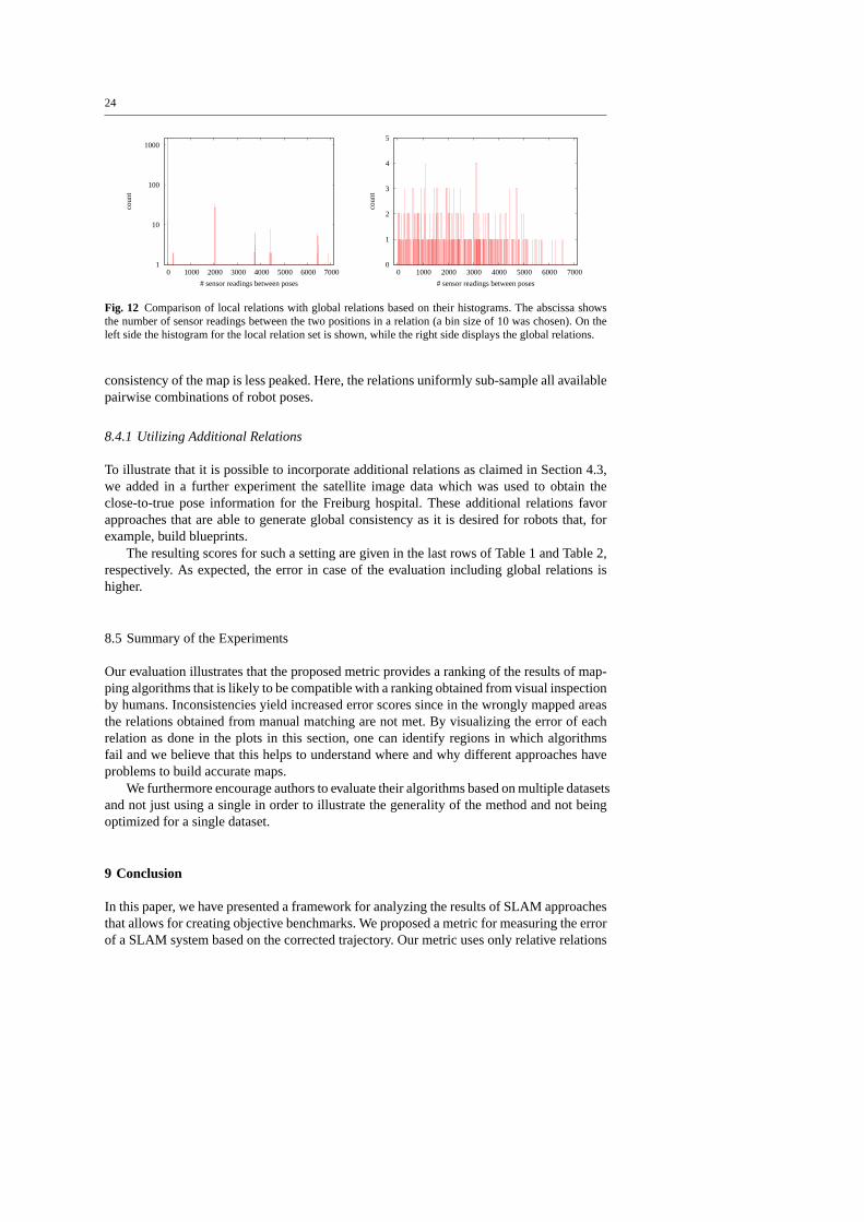
Fig. 12 Comparison of local relations with global relations based ontheir histograms. The abscissa showsthe number of sensor readings between the two positions in a relation (a bin size of 10 was chosen). On theleft side the histogram for the local relation set is shown, while the right side displays the global relations.

consistency of the map is less peaked. Here, the relations uniformly sub-sample all availablepairwise combinations of robot poses.

8.4.1 Utilizing Additional Relations

To illustrate that it is possible to incorporate additionalrelations as claimed in Section 4.3,we added in a further experiment the satellite image data which was used to obtain theclose-to-true pose information for the Freiburg hospital.These additional relations favorapproaches that are able to generate global consistency as it is desired for robots that, forexample, build blueprints.

The resulting scores for such a setting are given in the last rows of Table 1 and Table 2,respectively. As expected, the error in case of the evaluation including global relations ishigher.

8.5 Summary of the Experiments

Our evaluation illustrates that the proposed metric provides a ranking of the results of map-ping algorithms that is likely to be compatible with a ranking obtained from visual inspectionby humans. Inconsistencies yield increased error scores since in the wrongly mapped areasthe relations obtained from manual matching are not met. By visualizing the error of eachrelation as done in the plots in this section, one can identify regions in which algorithmsfail and we believe that this helps to understand where and why different approaches haveproblems to build accurate maps.

We furthermore encourage authors to evaluate their algorithms based on multiple datasetsand not just using a single in order to illustrate the generality of the method and not beingoptimized for a single dataset.

9 Conclusion

In this paper, we have presented a framework for analyzing the results of SLAM approachesthat allows for creating objective benchmarks. We proposeda metric for measuring the errorof a SLAM system based on the corrected trajectory. Our metric uses only relative relations

25

between poses and does not rely on a global reference frame. This overcomes serious short-comings of approaches using a global reference frame to compute the error. The metric evenallows for comparing SLAM approaches that use different estimation techniques or differentsensor modalities.

In addition to the proposed metric, we provide robotic datasets together with relativerelations between poses for benchmarking. These relationshave been obtained by manu-ally matching observations and yield a high matching accuracy. We present relations forself-recorded datasets with laser range finder data as well as for a set of log-files that arefrequently used in the SLAM community to evaluate approaches. In addition, we providean error analysis for three mapping systems including two modern laser-based SLAM ap-proaches, namely a graph-based approach as well as system based on a Rao-Blackwellizedparticle filter. We believe that our results are a valuable benchmark for SLAM researcherssince we provide a framework that allows for objectively andcomparably easy analyzingthe results of SLAM systems.

Acknowledgments

This work has partly been supported by the DFG under contractnumber SFB/TR-8 and theEuropean Commission under contract numbers FP6-2005-IST-6-RAWSEEDS, FP7-231888-EUROPA, and FP6-IST-045388-INDIGO. The authors gratefully thank Mike Bosse, PatrickBeeson, and Dirk Haehnel for providing the MIT Killian Court, the ACES, and the Intel Re-search Lab datasets.

References

[Amigoni et al., 2007] F. Amigoni, S. Gasparini, and M. Gini. Good experimental methodologies for roboticmapping: A proposal. InProc. of the IEEE Int. Conf. on Robotics & Automation (ICRA), 2007.

[Balagueret al., 2007] B. Balaguer, S. Carpin, and S. Balakirsky. Towards quantitative comparisons of robotalgorithms: Experiences with SLAM in simulation and real world systems. InIROS 2007 Workshop, 2007.

[Bar-Shalomet al., 2001] Y Bar-Shalom, X.R. Li, and T. Kirubarajan.Estimation with Application to Track-ing and Navigation. Jonh Wiley and Sons, 2001.

[Bonariniet al., 2006] A. Bonarini, W. Burgard, G. Fontana, M. Matteucci, D.G. Sorrenti, and J. D. Tar-dos. Rawseeds a project on SLAM benchmarking. InProceedings of the IROS’06 Workshop on Bench-marks in Robotics Research, 2006. available online at http://www.robot.uji.es/EURON/pdfs/Lecture NotesIROS06.pdf.

[Bosseet al., 2003] M. Bosse, P.M. Newman, J.J. Leonard, and S. Teller. An ALTAS framework for scalablemapping. InProc. of the IEEE Int. Conf. on Robotics & Automation (ICRA), pages 1899–1906, Taipei,Taiwan, 2003.

[Burgardet al., 2009] W. Burgard, C. Stachniss, G. Grisetti, B. Steder, R. Kummerle, C. Dornhege,M. Ruhnke, A. Kleiner, and J. D. Tardos. A comparison of slam algorithms based on a graph of rela-tions. InProc. of the Int. Conf. on Intelligent Robots and Systems (IROS), 2009. To appear.

[Canny, 1986] J. Canny. A computational approach to edge detection. IEEE Trans. Pattern Anal. Mach.Intell., 8(6):679–698, 1986.

[Censi, 2006] A. Censi. Scan matching in a probabilistic framework. In Proc. of the IEEE Int. Conf. onRobotics & Automation (ICRA), pages 2291–2296, 2006.

[Darpa, 2007] Darpa. Darpa Urban Challenge, 2007. http://www.darpa.mil/grandchallenge/.[Dellaertet al., 1998] F. Dellaert, D. Fox, W. Burgard, and S. Thrun. Monte carlo localization for mobile

robots. InProc. of the IEEE Int. Conf. on Robotics & Automation (ICRA), Leuven, Belgium, 1998.[Dellaert, 2005] F. Dellaert. Square Root SAM. InProc. of Robotics: Science and Systems (RSS), pages

177–184, Cambridge, MA, USA, 2005.[Dissanayakeet al., 2000] G. Dissanayake, H. Durrant-Whyte, and T. Bailey. A computationally efficient

solution to the simultaneous localisation and map building (SLAM) problem. In Proc. of the IEEEInt. Conf. on Robotics & Automation (ICRA), pages 1009–1014, 2000.

26

[Doucetet al., 2001] A. Doucet, N. de Freitas, and N. Gordan, editors.Sequential Monte-Carlo Methods inPractice. Springer Verlag, 2001.

[Duckettet al., 2002] T. Duckett, S. Marsland, and J. Shapiro. Fast, on-line learning of globally consistentmaps.Autonomous Robots, 12(3):287 – 300, 2002.

[EPFL and IROS, 2002] EPFL and IROS. Cleaning Robot Contest,2002.http://robotika.cz/competitions/cleaning2002/en.

[ESA, 2008] ESA. Lunar robotics challenge, 2008. http://www.esa.int/esaCP/SEM4GKRTKMFindex 0.html.[Estradaet al., 2005] C. Estrada, J. Neira, and J.D. Tardos. Hierachical SLAM: Real-time accurate mapping

of large environments.IEEE Transactions on Robotics, 21(4):588–596, 2005.[Eusticeet al., 2005a] R. Eustice, H. Singh, and J.J. Leonard. Exactly sparse delayed-state filters. InProc. of

the IEEE Int. Conf. on Robotics & Automation (ICRA), pages 2428–2435, 2005.[Eusticeet al., 2005b] R. Eustice, M. Walter, and J.J. Leonard. Sparse extended information filters: Insights

into sparsification. InProc. of the Int. Conf. on Intelligent Robots and Systems (IROS), pages 641–648,Edmonton, Cananda, 2005.

[Freseet al., 2005] U. Frese, P. Larsson, and T. Duckett. A multilevel relaxation algorithm for simultaneouslocalisation and mapping.IEEE Transactions on Robotics, 21(2):1–12, 2005.

[Frese, 2006] U. Frese. Treemap: Ano(logn) algorithm for indoor simultaneous localization and mapping.Autonomous Robots, 21(2):103–122, 2006.

[Frese, 2008] U. Frese. Dlr spatial cognition data set. http://www.informatik.uni-bremen.de/agebv/en/DlrSpatialCognitionDataSet, 2008.

[Fruh and Zakhor, 2004] C. Fruh and A. Zakhor. An automated method for large-scale, ground-based citymodel acquisition.International Journal of Computer Vision, 60:5–24, 2004.

[Grisetti et al., 2007a] G. Grisetti, S. Grzonka, C. Stachniss, P. Pfaff, andW. Burgard. Efficient estimationof accurate maximum likelihood maps in 3D. InProc. of the Int. Conf. on Intelligent Robots and Systems(IROS), San Diego, CA, USA, 2007.

[Grisetti et al., 2007b] G. Grisetti, C. Stachniss, and W. Burgard. Improved techniques for grid mappingwith rao-blackwellized particle filters.IEEE Transactions on Robotics, 23:34–46, 2007.

[Grisetti et al., 2007c] G. Grisetti, C. Stachniss, S. Grzonka, and W. Burgard. A tree parameterization forefficiently computing maximum likelihood maps using gradient descent. InProc. of Robotics: Scienceand Systems (RSS), 2007.

[Gutmann and Konolige, 1999] J.-S. Gutmann and K. Konolige. Incremental mapping of large cyclic envi-ronments. InProc. of the IEEE Int. Symposium on Computational Intelligence in Robotics and Automation(CIRA), 1999.

[Hahnelet al., 2003] D. Hahnel, W. Burgard, D. Fox, and S. Thrun. An efficient FastSLAMalgorithm forgenerating maps of large-scale cyclic environments from raw laser range measurements. InProc. of theInt. Conf. on Intelligent Robots and Systems (IROS), pages 206–211, 2003.

[Hermosilloet al., 2003] J. Hermosillo, C. Pradalier, S. Sekhavat, C. Laugier,and G. Baille. Towards motionautonomy of a bi-steerable car: Experimental issues from map-building to trajectory execution. InProc. ofthe IEEE Int. Conf. on Robotics & Automation (ICRA), 2003.

[Hooveret al., 1996] A. Hoover, G. Jean-Baptiste, X. Jiang, P. J. Flynn, H.Bunke, D. B. Goldgof, K. K.Bowyer, D. W. Eggert, A. W. Fitzgibbon, and R. B. Fisher. An experimental comparison of range imagesegmentation algorithms.IEEE Transactions on Pattern Analysis and Machine Intelligence, 18(7):673–689, 1996.

[Howard and Roy, 2003] A. Howard and N. Roy. Radish: The robotics data set repository, standard data setsfor the robotics community, 2003. http://radish.sourceforge.net/.

[Julieret al., 1995] S. Julier, J. Uhlmann, and H. Durrant-Whyte. A new approach for filtering nonlinearsystems. InProc. of the American Control Conference, pages 1628–1632, 1995.

[Kaesset al., 2007] M. Kaess, A. Ranganathan, and F. Dellaert. iSAM: Fastincremental smoothing andmapping with efficient data association. InProc. of the IEEE Int. Conf. on Robotics & Automation (ICRA),2007.

[Kummerleet al., 2009] R. Kummerle, B. Steder, C. Dornhege, A. Kleiner, G. Grisetti, and W. Burgard.Large scale graph-based SLAM using aerial images as prior information. InProc. of Robotics: Scienceand Systems (RSS), 2009.

[Leonard and Durrant-Whyte, 1991] J.J. Leonard and H.F. Durrant-Whyte. Mobile robot localization bytracking geometric beacons.IEEE Transactions on Robotics and Automation, 7(4):376–382, 1991.

[Lu and Milios, 1994] F. Lu and E. Milios. Robot pose estimation in unknown environments by matching2d range scans. InIEEE Computer Vision and Pattern Recognition Conference (CVPR), pages 935–938,1994.

[Lu and Milios, 1997] F. Lu and E. Milios. Globally consistent range scan alignment for environment map-ping. Autonomous Robots, 4:333–349, 1997.

27

[Montemerloet al., 2003] M. Montemerlo, S. Thrun, D. Koller, and B. Wegbreit. FastSLAM 2.0: An im-proved particle filtering algorithm for simultaneous localization and mapping that provably converges. InProc. of the Int. Conf. on Artificial Intelligence (IJCAI), pages 1151–1156, 2003.

[Nuchteret al., 2005] A. Nuchter, K. Lingemann, J. Hertzberg, and H. Surmann. 6d SLAM with approxi-mate data association. InProc. of the 12th Int. Conference on Advanced Robotics (ICAR), pages 242–249,2005.

[Olsonet al., 2006] E. Olson, J. Leonard, and S. Teller. Fast iterative optimization of pose graphs with poorinitial estimates. InProc. of the IEEE Int. Conf. on Robotics & Automation (ICRA), pages 2262–2269,2006.

[Olson, 2008] E. Olson.Robust and Efficient Robotic Mapping. PhD thesis, Massachusetts Institute ofTechnology, Cambridge, MA, USA, 2008.

[Pfaff et al., 2006] P. Pfaff, W. Burgard, and D. Fox. Robust monte-carlo localization using adaptive like-lihood models. In H.I. Christiensen, editor,European Robotics Symposium 2006, volume 22 ofSTARSpringer tracts in advanced robotics, pages 181–194. Springer-Verlag Berlin Heidelberg, Germany, 2006.

[Ranganathanet al., 2007] A. Ranganathan, M. Kaess, and F. Dellaert. Loopy sam. In Proc. of theInt. Conf. on Artificial Intelligence (IJCAI), 2007.

[RoboCup Federation, 2009] RoboCup Federation. RoboCup Competitions, 2009. http://www.robocup.org.[Scharstein and Szeliski, 2002] D. Scharstein and R. Szeliski. Middlebury stereo vision page, 2002.

http://www. middlebury. edu/stereo.[Smith and Cheeseman, 1986] R. C. Smith and P. Cheeseman. On the representation and estimation of spa-

tial uncertainty.International Journal of Robotics Research, 5(4):56–68, 1986.[Smith et al., 1990] R. Smith, M. Self, and P. Cheeseman. Estimating uncertain spatial realtionships in

robotics. In I. Cox and G. Wilfong, editors,Autonomous Robot Vehicles, pages 167–193. Springer Verlag,1990.

[Stachnisset al., 2007a] C. Stachniss, U. Frese, and G. Grisetti. OpenSLAM.org – give your algorithm tothe community. http://www.openslam.org, 2007.

[Stachnisset al., 2007b] C. Stachniss, G. Grisetti, N. Roy, and W. Burgard. Evaluation of gaussian proposaldistributions for mapping with rao-blackwellized particlefilters. In Proc. of the Int. Conf. on IntelligentRobots and Systems (IROS), 2007.

[Symeo GmbH, 2008] Symeo GmbH. http://www.symeo.de, 2008.[Thrun and colleagues, 2006] S. Thrun and colleagues. Winning the darpa grand challenge.Journal on Field

Robotics, 2006.[Thrunet al., 2004] S. Thrun, Y. Liu, D. Koller, A.Y. Ng, Z. Ghahramani, andH. Durrant-Whyte. Simultane-

ous localization and mapping with sparse extended information filters. Int. Journal of Robotics Research,23(7/8):693–716, 2004.

[Thrunet al., 2005] S. Thrun, W. Burgard, and D. Fox.Probabilistic Robotics. MIT Press, 2005.[Thrun, 2001] S. Thrun. An online mapping algorithm for teams of mobile robots.Int. Journal of Robotics

Research, 20(5):335–363, 2001.[Torralbaet al., 2007] A. Torralba, K. P. Murphy, and W. T. Freeman. Labelme: the open annotation tool,

2007. http://labelme.csail.mit.edu/.[Uhlmann, 1995] J. Uhlmann.Dynamic Map Building and Localization: New Theoretical Foundations. PhD

thesis, University of Oxford, 1995.[Wulf et al., 2008] O. Wulf, A. Nuchter, J. Hertzberg, and B. Wagner. Benchmarking urban six-degree-of-

freedom simultaneous localization and mapping.Journal of Field Robotics, 25(3):148–163, 2008.[Yguel et al., 2007] M. Yguel, C.T.M. Keat, C. Braillon, C. Laugier, and O.Aycard. Dense mapping for

range sensors: Efficient algorithms and sparse representations. InProc. of Robotics: Science and Systems(RSS), 2007.