On maximum likelihood estimation in sparse - Deep Blue

Computational Statistics & Data Analysis 1 (1983) 3-15 North-Holland Publishing Company

On maximum likelihood estimation in sparse contingency tables

Morton B. BROWN Department of Biostatistics, University of Michigan, Ann Arbor, MI 48109, USA and Department of Statistics, Tel-Aviv University, Tel-Aviv, Israel

Camil FUCHS Department of Statistics, Tel-Aviv University, Tel-Aviv, lsrael and Department of Statistics, University of Haifa, Mt. Carmel, Haifa, Israel

Received September 1982 Revised December 1982

Abstract: Log-linear and logistic models can be fitted to data in contingency tables either by an iterative proportional fitting algorithm or by an iteratively reweighted Newton-Raphson algorithm. Both algorithms provide maximum likelihood (ML) estimates of the expected cell frequencies and of the parameters of the model. When random zeros occur in the contingency table, numerical problems may be encountered in obtaining the ML estimates when using one or both of the algorithms. Problems in the estimation of the model's parameters, expected cell frequencies and degrees of freedom are described. An explicit formula is given for the evaluation of the degrees of freedom.

Keywords: Log-linear model, Multiway contingency table, Sparse table, Newton-Raphson, Iterative proportional fitting, Logistic regression.

1. I n t r o d u c t i o n

The two common methods to obtain maximum likelihood (ML) estimates of the parameters of a log-linear model are to apply either an iterative proportional fitting (IPF) or an iteratively reweighted Newton -Raphson (NR) algorithm. When all cells in the frequency table have positive expected frequencies under the model fitted, both the expected frequencies and the parameter estimates are obtained from the IPF or N R solutions; also there is no difficulty in determining the degrees of freedom (df) of the chi-square test-of-fit of the model.

A sparse frequency table has many cell frequencies equal to zero and, as a result, one or more expected cell frequencies for a given model may be identically zero, In this article we discuss difficulties that may occur when

(a) estimating the expected cell frequencies (b) determining the df of the test-of-fit (c) obtaining the parameter estimates

of a log-linear model fitted to a sparse frequency table.

0167-9473/83/0000-0000/$03.00 © 1983 North-Holland

4 M.B. Brown, C. Fuchs / MLE in sparse tables

For both the NR and IPF algorithms there may be difficulties in identifying cells with zero expected values. Improper identification of such cells will also cause the degrees of freedom (df) for the test-of-fit of the log-linear model to be incorrectly calculated.

When the frequency table is sparse, an additional problem is the overparametrization of the model or, equivalently, the aliasing of design vectors in the log-linear model. Although the expected values of the cell frequencies are unique, the parameter estimates can differ when different implementations of the NR algorithm or of the matrix pivoting routine are used. In addition, the determination of the degrees of freedom also depends upon the number of nonestimable parameters. This number is often evaluated by determining the rank of a singular matrix which may be affected by problems of numerical accuracy. We present an explicit formula to evaluate the number of nonestimable parameters.

When the NR algorithm is used, the log-linear model is explicitly specified by the design matrix and by the inclusion or exclusion of cells with zero frequencies from the data input vector. The exclusion of a cell from the data input vector implicitly defines the cell as a structural zero.

2. ML estimation of expected values, parameters and degrees of freedom

The log-linear model can be expressed in matrix notation as

In F = XX

[5] where F is the vector of expected cell frequencies, h is the vector of parameters in the model, and X is the design matrix in which each row represents a cell.

Each h-term fulfils the constraints that its sum over each of its indices is zero. Furthermore, let f be the vector of observed frequencies and W be a diagonal matrix with F along the diagonal. The matrix W is a generalized inverse of the asymptotic variance matrix of In F.

When an index has two levels and represents a dependent variable, the log-linear model can be represented as a logistic model [3] with a vector of parameters to. The logistic parameters to are twice the corresponding log-linear parameters X.

2.1. Algorithms to obtain M L estimates

Maximum likelihood estimates of the expected cell frequencies under a specified log-linear model can be obtained either by an iterative proportional fitting (IPF) algorithm (see, e.g., [4]) or by an iteratively reweighted least squares algorithm such as a Newton-Raphson (NR) algorithm with the weights modified at each iteration (see, e.g., [9]).

The IPF algorithm is applied to the cell frequencies in the observed frequency table. Therefore, if the data are presented in any other form, such as individual data records, the computer program first forms the frequency table and the marginal subtables corresponding to the model configurations. Using these margi-

M.B. Brown, C. Fuchs / MLE in sparse tables 5

nal subtables the IPF algorithm iterates to obtain the ML expected values. The N e w t o n - R a p h s o n type of algorithm finds a set of parameter estimates 2~

such that

F = exp( X~ )

for which the partial derivatives of

with respect to the parameters X are simultaneously zero. These )~ are the maximum likelihood estimates [10]. Note that W is reevaluated at each iteration using the currently best estimates of the expected cell frequencies F.

The estimates of the parameters ~ of the logistic model can be obtained by the NR algorithm in a manner similar to that described above for the log-linear model.

2.2. Expected values

When there is a zero in a marginal configuration defined by a log-linear model, the cells comprising that marginal zero have expected values that are zero. The IPF algorithm sets the expected values for these cells to zero on the first iteration. However, if a cell that has a zero expected value does not correspond to a marginal zero, the IPF algorithm will not estimate the expected value as identically zero, al though the estimated expected value asymptotically approaches zero as more iterations are performed. The simplest example of this occurs in a 2 × 2 × 2 table when there are two cells with observed frequencies equal to zero but the two cells are in different rows, columns and layers. When the log-linear model that has all two-factors interactions but no three-factor interaction is fitted to the data, there are two zero expected frequencies. However, the IPF estimates of these expected frequencies converge very slowly to zero ([4], p. 70).

Programs implementing the NR algorithm apply the algorithm to the data vector that is read as input. When the data vector contains only the observed data (such as, case-by-case or nonzero cell frequencies), the vector f to which the algorithm is applied will not contain cells with observed frequencies equal to zero. Since the algori thm assumes implicitly that the sum of the observed frequencies is equal to the sum of the expected ones over all cells in the vector f (i.e., l ' f = I 'F ) , the expected frequencies of all cells that are not represented in the data vector are set equal to zero. That is, the cells that are omitted because they have zero observed frequencies will also have zero expected frequencies.

This error can be avoided by inserting into jr and X all cells with nonzero expected frequencies. Thus f must contain zeros for all cells with observed frequencies equal to zero but whose expected frequencies are nonzero. Hence the vec:or of cell frequencies to be used as input to the N R algorithm depends on the log-linear model to be fitted.

The above problem with observed zeros does not arise when the N R algorithm is used to fit a logistic model.


2.3. Parameter estimates

When there are no zero expected values, X can be estimated from the loga- rithms of the expected frequencies as in the ANOVA model which has one observation per cell. However, if the expected value of any cell is zero, In F is not defined for that cell. Parameter estimates can be obtained by solving the set of simultaneous equations

Y= XX

where Y is a column vector containing In F for all nonzero F. The parameter estimates 2~ and their asymptotic standard errors (ASEs) are

obtained as

X ~-- ( X t W X ) - i X t W y ( 1 )

since the ASEs of f, are equal to the square roots of the diagonal elements of ( X ' W X ) -~. When X ' W X is nonsingular, these estimates are identically those obtained by the N R algorithm at the last iteration.

When the model is overparametrized, X ' W X is singular. More than one solution for 2( is possible. We recommend solving for the parameter estimates of lower-order terms and setting the coefficients of the higher-order aliased terms to zero.

Even when X ' W X is singular, all parameter estimates obtained by the NR-type algorithm may be nonzero since the algorithm can modify different subsets of the parameters at each iteration. One indication of overparametrization is when some ASEs are either very large or zero. We recommend that the estimates be obtained by re-solving for )k by (1) using the expected frequencies at the last iteration.

2.4. Degrees of freedom

When the frequency table is inseparable with respect to the model, the formula for degrees of freedom is

df = n c - n z - ( n p - nn)

where nc is the number of cells, in the table, n z is the number of cells with expected values equal to zero, n p is the number of parameters specified in the model and n n is the number of nonestimable parameters [4]. The number of cells n c is known, the number of zero expected values nz can usually be counted and the number of parameters n p c a n easily be evaluated. The number of nonestimable parameters can be obtained explicitly as described in the Appendix.

Alternatively, if the matrix X ' W X is formed, its rank is equal to r i p - n n. However there may be problems of numerical accuracy in the determination of the rank.

Incautious use of the N R algorithm in computer programs may result in the following kinds of errors when evaluating the degrees of freedom. The vector of frequencies f may have more than one entry per cell and therefore n c is overestimated. This error can be avoided by evaluating the df for both the model


of interest and for the saturated model - the difference in df between the two models is the df for the chi-square test of goodness-of-fit. Since the NR algorithm cannot produce an expected value that is exactly zero, a tolerance limit [2,6] must be set to identify any cells with 'zero' expected frequency; an incorrect tolerance limit may give an incorrect value for n z. Lastly the rank of the matrix X ' W X may be incorrectly evaluated. Hence care must be taken when evaluating the df for a sparse table.

3. An example of errors that arise in fitting models to sparse tables

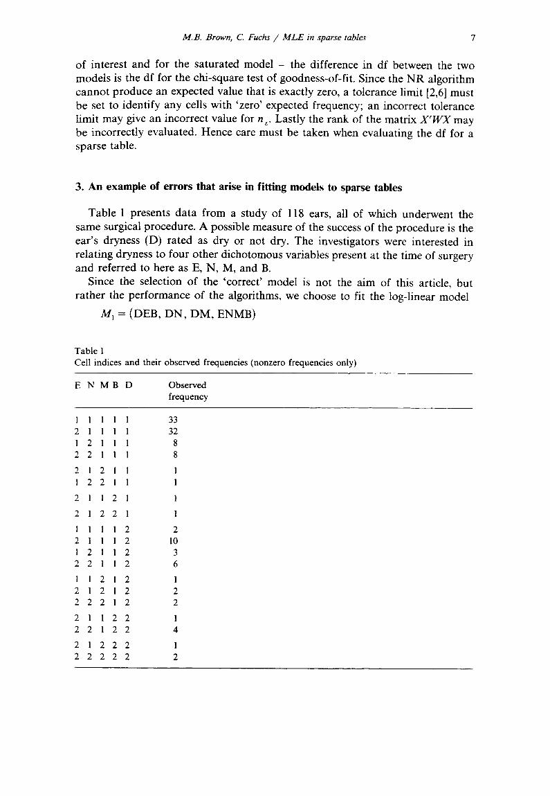
Table 1 presents data from a study of 118 ears, all of which underwent the same surgical procedure. A possible measure of the success of the procedure is the ear's dryness (D) rated as dry or not dry. The investigators were interested in relating dryness to four other dichotomous variables present at the time of surgery and referred to here as E, N, M, and B.

Since the selection of the 'correct' model is not the aim of this article, but rather the performance of the algorithms, we choose to fit the log-linear model

M~ = (DEB, DN, DM, ENMB)

Table 1 Cell indices and their observed frequencies (nonzero frequencies only)

E N M B D Observed frequency

1 1 1 1 1 33 2 1 1 1 1 32 1 2 1 1 1 8 2 2 1 1 1 8

2 1 2 1 1 1

1 2 2 1 1 1

2 1 1 2 1 1

2 1 2 2 1 1

1 1 1 1 2 2 2 1 1 1 2 10 1 2 1 1 2 3 2 2 1 1 2 6

1 1 2 1 2 1 2 1 2 1 2 2 2 2 2 1 2 2

2 1 1 2 2 1 2 2 1 2 2 4

2 1 2 2 2 1 2 2 2 2 2 2


where DEB, DN, DM, ENMB are the configurations that define the sufficient statistics and the marginal subtables that are used in the IPF iterations. The model is hierarchical but not direct [4].

The original table contains 13 random zeros. The marginal DEB table (obtained by summing over N and M) contains two zero frequencies and the marginal ENMB table contains four zero frequencies. The zeros in the marginal subtables force eight cells to have expected frequencies equal to zero under model M 1 •

If dryness (D) is treated as a dependent variable, the above model M~ corresponds to a logistic model where the logit of D is a function of the main effects of all four other variables and of the interaction between E and B. This logistic model will be referred to as L~. Each term in L I corresponds to a term in M~: to to A D, to E to A ED, ton to AND, toM to A MD, toB to A BD and toEB to A EBD where

the superscript identifies the term in the appropriate model. If all expected values were nonzero, each estimated to-term would be twice the corresponding A-term.

The log-linear model M~ wasfi t ted to the data by (a) IPF using BMDP4F [5], (b) NR using GLIM [1] a n d / o r a program based on Haberman [9],

and the logistic model L~ was fitted by (c) NR using GLIM or BMDPLR [7]. All computations were performed in single precision on the CDC 6600 com-

puter at Tel-Aviv University. The CDC 6600 computer has a 60-bit word, 48-bit mantissa, which produces at least 12 digits of numerical accuracy.

3.1. Expected values

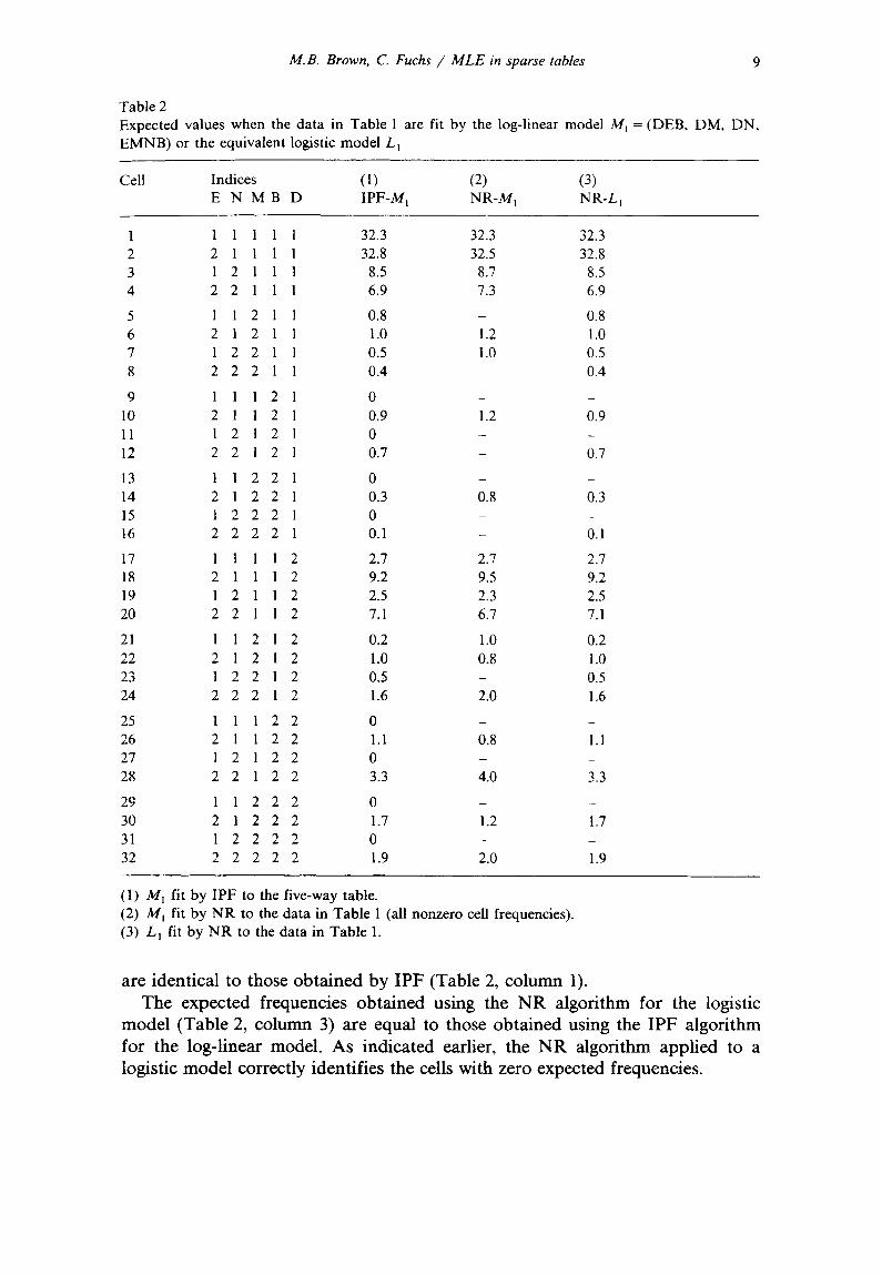
Table 2 presents the expected values obtained by: (1) Using IPF to fit the log-linear model M~ to the observed frequencies in all

cells. (2) Using

Table 1 (i.e., (3) Using

Table 1. Using the

NR to fit the log-linear model M~ to the observed frequencies in to all nonzero observed frequencies). N R to fit the logistic model L~ to the observed frequencies in

IPF algorithm eight-cells have expected values identically equal to zero (cells 9, 11, 13, 15, 25, 27, 29 and 31). Therefore the model can be fitted to the data with any or all of these cells defined as structural zeros. None of the other cells have expected values equal to zero although cells 5, 8, 12, 16 and 23 have observed zero frequencies.

When the model M~ is fitted by the NR algorithm to the data from Table l, the expected frequencies differ from those yielded by IPF. The N R values are identical to the ones obtained by applying the IPF algorithm to the data in the frequency table in which all observed zei'os are defined to be structural zeros. However, when the f vector is composed of the 19 observed cell frequencies in Table 1 and of the 5 zeros corresponding to the cells with zero observations but nonzero expected values, the expected frequencies obtained by the N R algorithm


T a b l e 2 Expected values when the data in T a b l e 1 are fit by the log-linear model M~

E M N B ) or the equivalent logistic model L~

= ( D E B , D M , D N ,

Cel l Indices (I) (2) (3) E N M B D I P F - M I N R - M I N R - L 1

1 1 1 1 1 1 32.3 32.3 32.3

2 2 1 1 1 1 32.8 32.5 32.8

3 1 2 1 1 1 8.5 8.7 8.5

4 2 2 1 1 1 6.9 7.3 6.9

5 I 1 2 1 1 0.8 - 0.8

6 2 1 2 1 1 1.0 1.2 1.0

7 1 2 2 1 1 0.5 1.0 0.5

8 2 2 2 1 1 0.4 - 0.4

9 1 1 1 2 1 0 - -

10 2 1 1 2 1 0.9 1.2 0.9

11 1 2 1 2 1 0 - -

12 2 2 1 2 1 0.7 - 0.7

13 1 1 2 2 1 0 - -

14 2 1 2 2 1 0.3 0.8 0.3

15 1 2 2 2 1 0 - -

16 2 2 2 2 1 0.1 - 0.1

17 1 1 1 1 2 2.7 2.7 2.7

18 2 1 1 1 2 9.2 9.5 9.2

19 1 2 1 1 2 2.5 2.3 2.5

20 2 2 1 1 2 7.1 6.7 7.1

21 1 1 2 1 2 0.2 1.0 0.2

22 2 1 2 1 2 1.0 0.8 1.0

23 1 2 2 1 2 0.5 - 0.5

24 2 2 2 1 2 1.6 2.0 1.6

25 1 1 1 2 2 0 - -

26 2 1 1 2 2 1.1 0.8 1.1

27 1 2 1 2 2 0 - -

28 2 2 1 2 2 3.3 4.0 3.3

29 1 1 2 2 2 0 - -

30 2 1 2 2 2 1.7 1.2 1.7

31 1 2 2 2 2 0 - -

32 2 2 2 2 2 1.9 2.0 1.9

(1) M I fit b y I P F to the f ive -way table .

(2) M1 fit b y N R to the data in T a b l e 1 (all n o n z e r o cell frequencies). (3) L 3 fit b y N R to the data in T a b l e 1.

are identical to those obtained by IPF (Table 2, column 1). The expected frequencies obtained using the NR algorithm for the logistic

model (Table 2, column 3) are equal to those obtained using the IPF algorithm for the log-linear model. As indicated earlier, the NR algorithm applied to a logistic model correctly identifies the cells with zero expected frequencies.


3. 2. Parameter estimates and degrees of freedom

Let us first exialuate the df for the model

M 1 = (ENMB, DEB, DN, DM).

There are 32 cells (no), eight of which have zero expected values (nz). The number of parameters in the model is 22 (the mean effect, five main effects, 10 two-factor interactions, five three-factor interactions and one four-factor interaction). However, five parameters are nonestimable. Therefore the df are

df = 3 2 - 8 - ( 2 2 - 5 ) = 7.

(Using the explicit formula described in the Appendix, the values of np(X z) - nn(~ z) are zeros for ~EB, ~DEB, ~ENB, ~EMB, ~ENMB and one for all other effects in the model.)

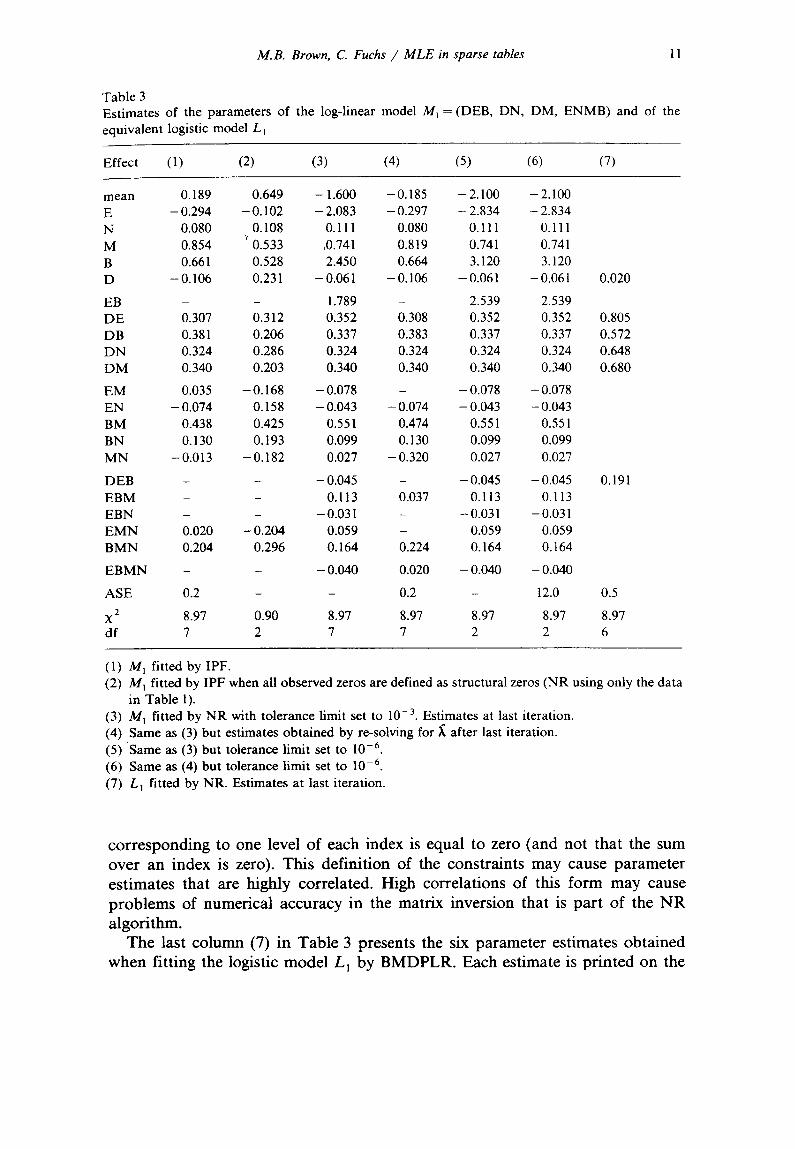
The parameter estimates of the log-linear model fitted by the IPF algorithm to data in sparse tables are obtained as

( x'wx)-'x'wr

where Y = In F at the last iteration of the IPF algorithm. Since Mt is overparametrized, X ' W X is singular. The matrix sweeping (pivoting) routine used by BMDP4F does not pivot on the five effects XEB, ADEB, AENB, hEMB and AENMB. The first column in Table 3 reports the estimates obtained for the other 17 parameters. The magnitude of a typical asymptotic standard error for a parameter estimate is given by the ASE in Table 3.

The solution produced by N R when the input data are the nonzero frequencies only (Table 3, column 2) is the same as that obtained by BMDP4F when all 13 cells with observed frequencies equal to zero are defined as structural zeros. Although the same number of parameters are estimated as in the first column, the estimates of all the parameters differ between the two analyses. The df are 2 since now there are effectively five fewer cells in the table.

Columns 3 and 4 in Table 3 present NR solutions produced at the two stages (at the end of the NR iterations and after re-solving using the expected values from the N R solution) when the tolerance limit [6] used for pivoting is 10 -3. Again five parameters are not estimated but they differ from those in column 1. Therefore some of the parameter estimates agree with those of IPF in column 1 but others differ; the parameter estimates that differ are aliased with one or more nonestimated parameters.

Columns 5 and 6 present a second pair of N R solutions when the tolerance limit for pivoting is set to 10 -6 . This tolerance limit is not sufficient to prevent pivoting on the nonestimable parameters. Therefore all parameters are estimated, but many of the ASEs are very large. Since the rank of X ' W X is overestimated (by 5 in our example), the calculated degrees of freedom are also in error (too small by 5).

Note: GLIM produces a different set of parameter estimates for both log-linear and logistic models. The constraints used by GLIM are that the parameter


Tab le 3 Es t imates of the parameters of the log-l inear model Mt

equ iva len t logistic model L I

= (DEB, DN, DM, E N M B ) and of the

Effect (1) (2) (3) (4) (5) (6) (7)

m e a n 0.189 0.649 - 1.600 - 0 . 1 8 5 - 2 . 1 0 0 - 2 . 1 0 0

E - 0 . 2 9 4 - 0 . 1 0 2 - 2 . 0 8 3 - 0 . 2 9 7 - 2 . 8 3 4 - 2 . 8 3 4

N 0.080 0.108 0.111 0.080 0.111 0.111 "t

M 0.854 0.533 ,0.741 0.819 0.741 0.741

B 0.661 0.528 2.450 0.664 3.120 3.120

D - 0 . 1 0 6 0.231 - 0 . 0 6 1 - 0 . 1 0 6 - 0 . 0 6 1 - 0 . 0 6 1 0.020

EB - - 1.789 - 2.539 2.539

D E 0.307 0.312 0.352 0.308 0.352 0.352 0.805

DB 0.381 0.206 0.337 0.383 0.337 0.337 0.572

D N 0.324 0.286 0.324 0.324 0.324 0.324 0.648

D M 0.340 0.203 0.340 0.340 0.340 0.340 0.680

E M 0.035 - 0.168 - 0.078 - - 0.078 - 0.078

E N - 0.074 0.158 - 0.043 - 0.074 - 0.043 - 0.043

BM 0.438 0.425 0.551 0.474 0.551 0.551

BN 0.130 0.193 0.099 0.130 0.099 0.099

M N - 0.013 - 0.182 0.027 - 0.320 0.027 0.027

D E B - - - 0 . 0 4 5 - - 0 . 0 4 5 - 0 . 0 4 5 0.191

EBM - - 0.113 0.037 0.113 0.113

EBN - - - 0.031 - - 0.031 - 0.031

E M N 0.020 - 0.204 0.059 - 0.059 0.059

B M N 0.204 0.296 0.164 0.224 0.164 0. i 64

E B M N - - - 0.040 0.020 - 0.040 - 0.040

A S E 0.2 - - 0.2 - 12.0 0.5

X 2 8.97 0.90 8.97 8.97 8.97 8.97 8.97

df 7 2 7 7 2 2 6

(1) M~ fitted by IPF.

(2) M I fit ted by IPF when all observed zeros are defined as s t ructural zeros ( N R us ing only the data

in Tab le 1).

(3) Mt fitted by N R with to le rance l imit set to 10 -3. Est imates at last i teration.

(4) Same as (3) bu t est imates ob t a ined by re-solving for A after last i teration.

(5) S a m e as (3) bu t tolerance l imit set t o 10 - 6 .

(6) Same as (4) bu t tolerance l imit set to 10 -6 .

(7) L I fitted by NR. Est imates at last i terat ion.

corresponding to one level of each index is equal to zero (and not that the sum over an index is zero). This definition of the constraints may cause parameter estimates that are highly correlated. High correlations of this form may cause problems of numerical accuracy in the matrix inversion that is part of the NR algorithm.

The last column (7) in Table 3 presents the six parameter estimates obtained when fitting the logistic model L 1 by BMDPLR. Each estimate is printed on the


line that corresponds to the equivalent term in model MI: w to ~D, wE t o ~DE, etc. This program does not re-solve for the parameter estimates after the last iteration. Therefore all parameter estimates are nonzero although w EB is aliased with three others, w E, W a and w. Two estimates w N and w M are, as expected, equal to twice the estimate of kDN and X DM respectively.

4. Discuss ion

When using the NR algorithm, the vector of frequencies used as input must include all cells but those having zero expected values under the model to be fitted. Cells with zero observed frequencies should be included unless their expected values under the log-linear model are zero. The parameter estimates should be obtained by re-solving for the estimates using the expected frequencies from the last iteration. The degrees of freedom may be computed using the rank of X ' W X but there may be a loss of accuracy if the wrong tolerance limit is used. The explicit formula given in the Appendix can be used instead.

When parameter estimates are aliased with others, problems in interpretation of the coefficients arise. We choose to retain the lower order parameter estimates among those that are aliased and to omit (set to zero) the higher order estimates. Algorithms that do not choose among the aliased parameter estimates produce estimates with very large asymptotic standard errors.

When the number of estimable parameters is less than the number of parameters, it is not possible to replace the model by the model excluding the nonestimable parameters and then expect to obtain the same results. For example, in Mt there are five nonestimable parameters. A model excluding the five nonestimable parameters is

M 2 = (DM, DN, ENM, NMB).

When this model is fitted to the data, the chi-square statistic is 15.24 with 15 df as compared to 8.97 with 7 df when model M l is fitted. The difference in df is due in part to the fact that fitting model M 2 produces no zero expected values whereas fitting M I creates 8 zeros. That is, the difference in df between two nested models is also affected by the difference in the number of zero expected values produced by the two models. The models M 1 and M 2 do not differ in the parameters estimated, but do differ in the chi-square tests-of-fit and dfs. Therefore, the difference between their chi-squares is not a test solely for the difference in estimable parameters between the two models; what is being tested is the difference in the lack-of-fit between the two models.

Additionally, the difference in df of two models that differ by a single effect may exceed the number of parameters associated with that effect. For example, when the model

M 3 = (B, ENMD)

is fitted to the data, six cells have zero expected values. Therefore

df (M3)= 3 2 - 6 - ( 1 7 - 3 )= 12.

M.B. Brown, C. Fuchs / M L E in sparse tables 13

However, if the model

M 4 ~" (B, ENM, END, EMD, NMD)

is fitted, there are no zero expected values and

df ( M 4 ) = 3 2 - 0 - ( 1 6 - 0) = 16.

Models M 3 and M 4 differ in only one effect ?~ENMD that defines a single parameter; therefore their df's should differ by one. The df's differ by four (and not one) because the addition of ~ENMD caused six zero expected values that resulted in three parameters becoming aliased with other parameters.

Both the IPF and the NR algorithms can produce the maximum likelihood estimates in sparse contingency tables. However, it is necessary to be aware of the numerical and conceptual problems that can arise when using the algorithms to fit log-linear models. Due to the rapid proliferation of new computer programs to fit these models, we recommend that the results from one program be cross-validated against the results from another, preferably one using a different algorithm.

Although proper implementation of both algorithms yields identical estimates for the class of hierarchical models described in this paper, the choice of which algorithm is preferable depends on the characteristics of the problem and of the computational facilities available. In general, if the model is direct and there are no structural zeros, the expected values can be stated explicitly and the IPF algorithm requires only one iteration. Otherwise, its rate of convergence is linear. In all cases the rate of convergence of the N R algorithm is quadratic [11]. However, the NR algorithm requires that a p x p covariance matrix be formed at each iteration, where p is the number of parameters to be estimated. If p is large, the computation of the covariance matrix will offset any gain due to fewer iterations. There are other classes of models for which the IPF algorithm is either very slow to converge, such as when the categories are ordered, or inapplicable, such as when the model is not hierarchical.

If all expected values in a sparse frequency table are small, the asymptotic properties of the maximum likelihood estimates and the chi-square statistics cannot be assumed to hold. Haberman [8] shows that the asymptotic properties are applicable when both the sample size and the number of cells in the table are large, even if individual expected frequencies are small. In addition, the test of the difference between two models is more robust than each of the tests of the individual models (Haberman, personal communication).

Appendix - An explicit formula for the number of nonestimable parameters

Let kz represent an effect in the log-linear model. Form the marginal subtable T O corresponding to the configuration Z. Let n0(k z) = number of zeros in table To, n~(k z) = number of zeros in all subtables formed by collapsing T O over exactly

one index in Z,


n2(~k z) = number of zeros in all subtables formed by collapsing T o over exactly two indices in Z,

n k (~z) = number of zeros in all subtables formed by collapsing To over exactly k indices in Z.

In the above, as soon as n i (~ z) is zero for any i, then nj (~ z) is zero for a l l j > i. The number of nonest imable parameters in ~z is

n o ( X z ) = , , 0 ( X z ) - n , ( X z ) + n 2 ( X z) . . . . + . . . .

The total number of nonestimable parameters is

no=En°(X z) where the summation is over all terms in the log-linear model.

The df can now be calculated as

df = n c - n z - ( n p - n , ) .

The above was derived empirically and is implemented in BMDP4F [5]. We have not as yet found any problems for which the above calculation of df is not correct.

Acknowledgements

Special thanks are due to Professor Y. Sadeh and Dr. E. Berko from the ENT Department, Meir Hospital, Kfar Saba, Israel, for permission to use the data in our example and to Professor Gad Nathan of the Department of Statistics, Hebrew University, for his assistance. Support for this research was provided in part by a subcontract from BMDP Statistical Software, Inc.

References

[ 1 ] R.J. Baker and J.A. Nelder, General Linear Interactive Modeling (GLIM). Release 3 (Numerical Algorithms Group, Oxford, 1978).

[2] K.N. Berk, Tolerance and condition in regression computations, J. Amer. Statist. Assoc. 72 (1977) 863-866.

[3] Y.M.M. Bishop, Full contingency tables, logits and split contingency tables, Biometrics 25 (1969) 545-562.

[4] Y.M.M. Bishop, S.E. Fienberg and P.W. Holland, Discrete Multivariate Analysis: Theory and Practice, 2nd ed. (MIT Press, Cambridge, MA, 1976).

[5] M.B. Brown, P4F - Two-way and multiway frequency measures of association and the log-linear model (complete and incomplete tables), in: W.J. Dixon (Ed.), BMDP Statistical Software (University of California Press, Los Angeles, 1981) 143-206.

[6] M.A. Efroymson, Multiple regression analysis, in: A. Ralston and H. Wilf (Eds.), Mathematical Methods for Digital Computers (John Wiley, New York, 1960) 191-203.

[7] L. Engelman, PLR - Stepwise logistic regression, in: W.J. Dixon (Ed.), BMDP Statistical Software (University of California Press, Los Angeles, 1981) 330-344.


[8] S.J. Haberman, Log-linear models and frequency tables with small expected cell counts, Annals of Statistics 5 (1977) 1148-1169.

[9] S.J. Haberman, Analysis of Qualitative Data - Vol 2, New Developments (Academic Press, New York, 1979).

[10] R.J. Jennrich and R.H. Moore, Maximum likelihood estimation by means of nonlinear least squares, in: Proceedings of the Statistical Computing Section, American Statistical Association (1975) 57-65.

[11] W.J. Kennedy, Jr. and J.E. Gentle, Statistical Computing (Marcel Dekker, New York, 1980).

Documents

On maximum likelihood estimation in sparse - Deep Blue