On-Line Nonlinear Dynamic Data Reconciliation Using Extended Kalman Filtering ...€¦ · · 2018-02-20Iran. J. Chem. Chem. Eng. Vol. 28, No. 3, 2009 1 On-Line Nonlinear Dynamic

Iran. J. Chem. Chem. Eng. Vol. 28, No. 3, 2009

1

On-Line Nonlinear Dynamic Data Reconciliation

Using Extended Kalman Filtering: Application to a

Distillation Column and a CSTR

Farzi, Ali

Department of Chemical Engineering, Faculty of Chemistry, University of Tabriz, Tabriz, I.R. IRAN

Mehrabani-Zeinabad, Arjomand*+

Department of Chemical Engineering, Isfahan University of Technology, 84156-83111 Isfahan, I.R. IRAN

Bozorgmehry Boozarjomehry, Ramin

Department of Chemical Engineering and Petroleum, Sharif University of Technology, Tehran, I.R. IRAN

ABSTRACT: Extended Kalman Filtering (EKF) is a nonlinear dynamic data reconciliation

(NDDR) method. One of its main advantages is its suitability for on-line applications. This paper

presents an on-line NDDR method using EKF. It is implemented for two case studies, temperature

measurements of a distillation column and concentration measurements of a CSTR. In each

time step, random numbers with zero mean and specified variance were added to simulated results

by a random number generator. The generated data are transferred on-line to a developed data

reconciliation software. The software performs NDDR on received data using EKF method.

Comparison of data reconciliation results with simulated measurements and true values

demonstrates a high reduction in measurement errors, while benefits high speed data reconciliation

process.

KEY WORDS: Data reconciliation, Nonlinear dynamic Data reconciliation, Extended kalman

filtering, Distillation column, CSTR, Object-oriented programming.

INTRODUCTION

Process plant measurements inherently contain

random and gross errors due to various sources such as

environmental, instrumental and human factors. These

data can affect performance of controlling systems and

decrease performance of controlled processing systems.

Thus these errors must be removed or alternatively their

effect on the performance of systems must be reduced.

Data Reconciliation (DR) is an optimization method

for elimination of random errors from measured data of

processing systems. It uses process models as constraint,

* To whom correspondence should be addressed.

+ E-mail: [email protected]

1021-9986/09/3/1 14/$/3.40

Iran. J. Chem. Chem. Eng. Farzi, A., et al. Vol. 28, No. 3, 2009

2

and statistical properties of measurements. DR can be

performed in both steady-state and dynamic conditions.

Many researches have been done within the framework of

Linear and Nonlinear Steady-State Data Reconciliation

(LSSDR and NSSDR). But enhancing the performance of

Linear and Nonlinear Dynamic DR (LDDR and NDDR)

in the contexts are still open and some methods have been

proposed for NDDR ([1-9]). Extended Kalman Filtering

is a most widely used method for nonlinear dynamic

processing systems such as control, diagnosis and data

reconciliation. It has a high performance and can be

applied on-line to different types of process measurements.

This method is not extensively used for NDDR and its

different aspects are not addressed. Only few papers are

devoted to EKF. Almasy [1] presented a method, namely

Dynamic Balancing, for dynamic reconciliation of state

measurements using linear models and accordingly linear

Kalman Filtering.

Some of the papers only compared EKF method with

other methods, [2 , 3]. Karajala et al. [9] used a recurrent

neural network for system identification and applied EKF

for data rectification via the trained network. Only two

conference papers are devoted to direct application of

Kalman Filtering in data reconciliation, [10,11]

This paper initially explains on-line NDDR using

EKF. Then application of on-line data reconciliation of

measurements using EKF on a distillation column and a

CSTR as two case studies is presented in order to show

its benefits. It is assumed that errors in measurements are

only random errors with zero mean and normal

distribution, N (0,σ).

THEORY

EKF is an important method for NDDR applications.

One of the forms of a process plant model that this

method can be applied on, is in the following form,

assuming no disturbances:

( ) wu,xfdt

dx+= (1)

( ) ε+= u,xhy (2)

where x, y and u are vectors of state variables,

measurements and input variables, respectively. Clearly,

f and h are non-linear functions of x and u. In physico-

chemical processes these equations are obtained by

conservation law of mass and energy.

The vector of modeling errors and disturbances is

shown by w and that of random errors in measurements is

shown by ε. To application of EKF, the above model

must be successively linearized around a known

neighborhood of a state vector at time t1, x(t1), namely x1:

( ) ( ) ( ) wu,xfuuJxxJdt

dx111f1f

1u1x++−+−≅ (3)

( ) ( ) ( ) ε++−+−≅ 111h1h u,xhuuJxxJy1u1x

( ) ( ) ε++−+−= 11h1h yuuJxxJ1u1x

where 1xfJ ,

1ufJ , 1xhJ and

1uhJ are Jacobian matrices

of f and h with respect to x and u at x1 and u1

respectively:

11

1u

11

1x

uu,xxx

f

uu,xxu

fx

fJ,

x

fJ

====

��

��

∂

∂=�

��

��

∂

∂= (4)

11

1u

11

1h

uu,xxx

h

uu,xxu

fx

hJ,

x

hJ

====

��

��

∂

∂=�

��

��

∂

∂=

1y is the vector of estimated values of measurements

at t=t1. In many cases u does not explicitly exist in

measurement equation (Eq. (2)). Thus h is usually an

function of x only, so Jh will be used in place of 1xhJ and

also 1f

J and 2fJ in place of

1xfJ and 1ufJ , respectively.

Because EKF can be applied on discrete state-space

models, Eq. (3) must be discretized. Assuming that 1f

J ,

x1, 2fJ , u and f(x1,u1) are constant within the time

domain of (k-1)T to kT, the final result is in the following

form:

[ ] [ ] [ ] wM1kBu1kAxkx ++−+−= (5)

[ ] [ ] ε+= kxJkz h

( )21

1f

f1

fTJ

JJIAB,eA −−==

( ) ( )[ ] 1111

f1 Buu,xfJxAIM1

−−−= −

where k is the time step for data acquisition and T is

the sampling time. The details of derivation are presented

in Appendix A.

Now, Eq. (5) can be used for EKF. Matrixes of 1f

J ,

2fJ and Jh can be calculated in each time step or in

some specified time steps, depending on the required

accuracy and nonlinearity level of the model equations.

Iran. J. Chem. Chem. Eng. On-Line Nonlinear Dynamic Data ... Vol. 28, No. 3, 2009

3

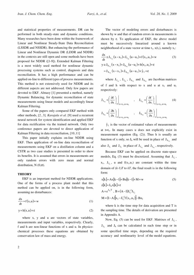
Fig. 1: Implemented distillation column.

For [ ]1kxx1 −= and [ ]1kuu1 −= , the above equation

can be simplified:

[ ] [ ] ( ) [ ] [ ]( )1ku,1kxfJIA1kxkx1

f1−−−+−= −

EKF steps are just like traditional KF except that in

each step a linearization on the model equations must be

done in order to get a linear set of state-space equations

for use in KF. The details of applying KF are not

presented here and can be found in the literature [12].

Now for on-line NDDR the following steps are necessary:

a) acquisition of new measurements from the plant,

b) calculation of Jacobian matrices of state and

measurements equations using estimated values in

previous step,

c) application of KF on refreshed linear system, and

calculation of estimates for states and measurements, the

reconciled measurements.

CASE STUDIES

The following two examples illustrate the performance

of EKF on NDDR of distillation column and a CSTR.

In both cases Kalman gain is dynamic and reaches a

steady state value within a certain time domain.

Case 1: NDDR by EKF applied to a methanol-water

distillation column

In order to illustrate the application of described

method, a distillation column is simulated.

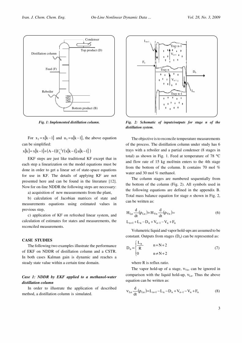
Fig. 2: Schematic of inputs/outputs for stage n of the

distillation system.

The objective is to reconcile temperature measurements

of the process. The distillation column under study has 6

trays with a reboiler and a partial condenser (8 stages in

total) as shown in Fig. 1. Feed at temperature of 78 °C

and flow rate of 15 kg mol/min enters to the 4th stage

from the bottom of the column. It contains 70 mol %

water and 30 mol % methanol.

The column stages are numbered sequentially from

the bottom of the column (Fig. 2). All symbols used in

the following equations are defined in the appendix B.

Total mass balance equation for stage n shown in Fig. 2,

can be written as:

( ) ( )=ρ+ρ VnVnLnLndt

dH

dt

dH (6)

nn1nnn1n FVVDLL +−+−+ −+

Volumetric liquid and vapor hold-ups are assumed to be

constant. Outputs from stages (Dn) can be represented as:

�

��

+≠

+==

2Nn0

2NnR

L

D

n

n (7)

where R is reflux ratio.

The vapor hold-up of a stage, νVn, can be ignored in

comparison with the liquid hold-up, νLn. Thus the above

equation can be written as:

( ) nn1nnn1nLnLn FVVDLLdt

d+−+−−=ρν −+ (8)

Condenser

Top product (D)Distillation column

Feed (F)

Reboiler

Bottom product (B)

Ln

Tray n-1

Vn-1

Dn

Fn

Ln+1

Vn+1

Tray n-1

Tray n


4

Mass balance equation for component i can also be

written in the following form, neglecting the vapor hold-

up:

( )Ln Ln i,n n 1 i,n 1 n i,n

dx L x L x

dt+ +ν ρ = − − (9)

n,fnn,in1n,i1nn,in xFyVyVxD +−+ −−

Assuming that vapor phase is ideal and variation of

liquid volume with pressure is negligible, the equilibrium

relation for the i-th component can be represented by:

*iiii PxPy γ= (10)

or

iii xKy = (11)

where

P

PK

*ii

i

γ= (12)

In practice, liquid and vapor phases on a given stage

are not in equilibrium. In order to determine the actual

rate of mass transfer, plate efficiency is implemented:

n,i1n,i

n,i1n,in

x)e(x

xxE

−

−=

+

+ (13)

where the parameter xi,n+1(e) is the composition of the

component i in liquid phase at equilibrium with vapor

leaving stage n. Its value can be replaced by Eq. (11).

( ) ��

��

� ρ+ρν=ρν

dt

dx

dt

dxx

dt

d Lnn,i

n,iLnLnn,iLnLn (14)

Multiplying Eq. (9) by En and using Eqs. (11) and

(14), finally the following result is obtained:

n,41n,in,3n,in,21n,in,1n,i

JxJxJxJdt

dx++−= −+ (15)

LnLnn

1nn,1

E

LJ

ρν= +

(16)

( ) ( )( )+

ρν

−−−+=

+

LnLnn

1nnnnnnn,inn,2

E

LLE1LDVKEJ (17)

dt

d1 Ln

Ln

ρ

ρ

LnLn

1n,i1nn,3

KVJ

ρν=

−− (18)

LnLn

n,fnn,4

xFJ

ρν= (19)

The last term in Eq. (17) can also be replaced by the

result of Eq. (8).

Heat balance equation is used to calculate vapor flow

rates:

( )�=

−−−− ++λ+m

1i

1n1n,ii,V1n,ii1nn,Fn TySyVhF (20)

( )++λ− ��==

+++

m

1i

nn,ii,Vn,iin

m

1i

1n1n,ii,L1n TySyVTxSL

=− ��==

m

1i

nn,ij,Ln

m

1i

nn,ii,Ln TxSLTxSD

n,cn,cn

m

l,i

n,c

m

1i

n,ii,VVnn,ii,LLn Qqdt

dTMySxS −+

�

�

��

�+ν+ν � �

=

For the computation of temperature variations in each

column stage within a time domain, the column model

can be completed by the implementation of equilibrium

equations. Summing of Eq. (10) over the number of

components results:

�=

γ=m

1i

*iii PxP (21)

Differentiating the above equation with respect to

time gives:

�=

��

��

� γ+γ+γ=

m

1i

i*ii

i*ii

*i

iidt

dPx

dt

dxP

dt

dPx

dt

dP (22)

The vapor pressure, *iP , is only a function of

temperature, while activity coefficient, γi, is a function

of temperature and components concentrations. By

differentiating from *iP with respect to T, substituting the

result into Eq. (22), assuming isobaric conditions,

rewriting it with respect to T, and noting the two

component system of water-methanol in this process, the

following equation concluded:

�=

��

��

� γ+γ

��

�� γ

+γ−γ

+γ

−=2

1i

i*ii

*i

ii

2*22

*22

1*11

*11

1

dt

dPx

dt

dPx

dt

dPxP

dt

dPxP

dt

dx

dt

dT (23)


5

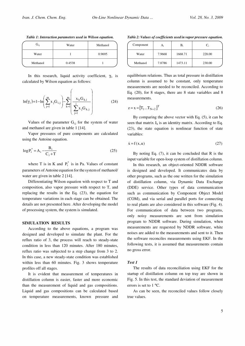
Table 1: Interaction parameters used in Wilson equation.

Gi,j Water Methanol

Water 1 0.9695

Methanol 0.4538 1

In this research, liquid activity coefficient, γi, is

calculated by Wilson equation as follows:

( ) ��

�=

=

=��

�

�

��

�

�

−��

��

�−=γ

m

1kj

1j

j,kj

i,kkm

1j

j,iji

Gx

GxGxln1ln (24)

Values of the parameter Gi,j for the system of water

and methanol are given in table 1 [14].

Vapor pressures of pure components are calculated

using the Antoine equation.

TC

BAPlog

i

ii

*i

+−= (25)

where T is in K and *iP is in Pa. Values of constant

parameters of Antoine equation for the systemof methanol/

water are given in table 2 [14].

Differentiating Wilson equation with respect to T and

composition, also vapor pressure with respect to T, and

replacing the results in the Eq. (23), the equation for

temperature variations in each stage can be obtained. The

details are not presented here. After developing the model

of processing system, the system is simulated.

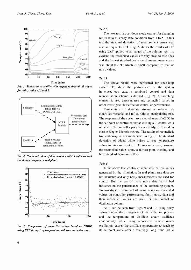
SIMULATION RESULTS

According to the above equations, a program was

designed and developed to simulate the plant. For the

reflux ratio of 3, the process will reach to steady-state

condition in less than 120 minutes. After 180 minutes,

reflux ratio was subjected to a step change from 3 to 2.

In this case, a new steady-state condition was established

within less than 60 minutes. Fig. 3 shows temperature

profiles off all stages.

It is evident that measurement of temperatures in

distillation column is easier, faster and more economic

than the measurement of liquid and gas compositions.

Liquid and gas compositions can be calculated based

on temperature measurements, known pressure and

Table 2: Values of coefficients used in vapor pressure equation.

Component Ai Bi Ci

Water 7.9668 1668.71 228.00

Methanol 7.8786 1473.11 230.00

equilibrium relations. Thus as total pressure in distillation

column is assumed to be constant, only temperature

measurements are needed to be reconciled. According to

Eq. (20), for 8 stages, there are 8 state variables and 8

measurements.

[ ]T2N1 T...Txz +== (26)

By comparing the above vector with Eq. (5), it can be

seen that matrix Jh is an identity matrix. According to Eq.

(23), the state equation is nonlinear function of state

variables:

)u,x(fx =� (27)

By noting Eq. (7), it can be concluded that R is the

input variable for open-loop system of distillation column.

In this research, an object-oriented NDDR software

is designed and developed. It communicates data by

other programs, such as the one written for the simulation

of distillation column, via Dynamic Data Exchange

(DDE) service. Other types of data communication

such as communication by Component Object Model

(COM), and via serial and parallel ports for connecting

to real plants are also considered in this software (Fig. 4).

For communication of data between two programs,

only noisy measurements are sent from simulation

program to NDDR software. During simulation, when

measurements are requested by NDDR software, white

noises are added to the measurements and sent to it. Then

the software reconciles measurements using EKF. In the

following tests, it is assumed that measurements contain

no gross error.

Test 1

The results of data reconciliation using EKF for the

startup of distillation column on top tray are shown in

Fig. 5. In this test, the standard deviation of measurement

errors is set to 1 °C.

As can be seen, the reconciled values follow closely

true values.


6

Fig. 3: Temperature profiles with respect to time of all stages

for reflux ratios of 3 and 2.

Fig. 4: Communication of data between NDDR software and

simulation program or real plant.

Fig. 5: Comparison of reconciled values based on NDDR

using EKF for top tray temperature with true and noisy ones.

Test 2

The next test in open-loop mode was set for changing

reflux ratio at steady-state condition from 3 to 5. In this

test the standard deviation of measurement errors was

also set equal to 1 °C. Fig. 6 shows the results of DR

using EKF applied to all stages of the column. As it is

evident, the reconciled values are very close to true ones

and the largest standard deviation of measurement errors

was about 0.2 °C which is small compared to that of

noisy values.

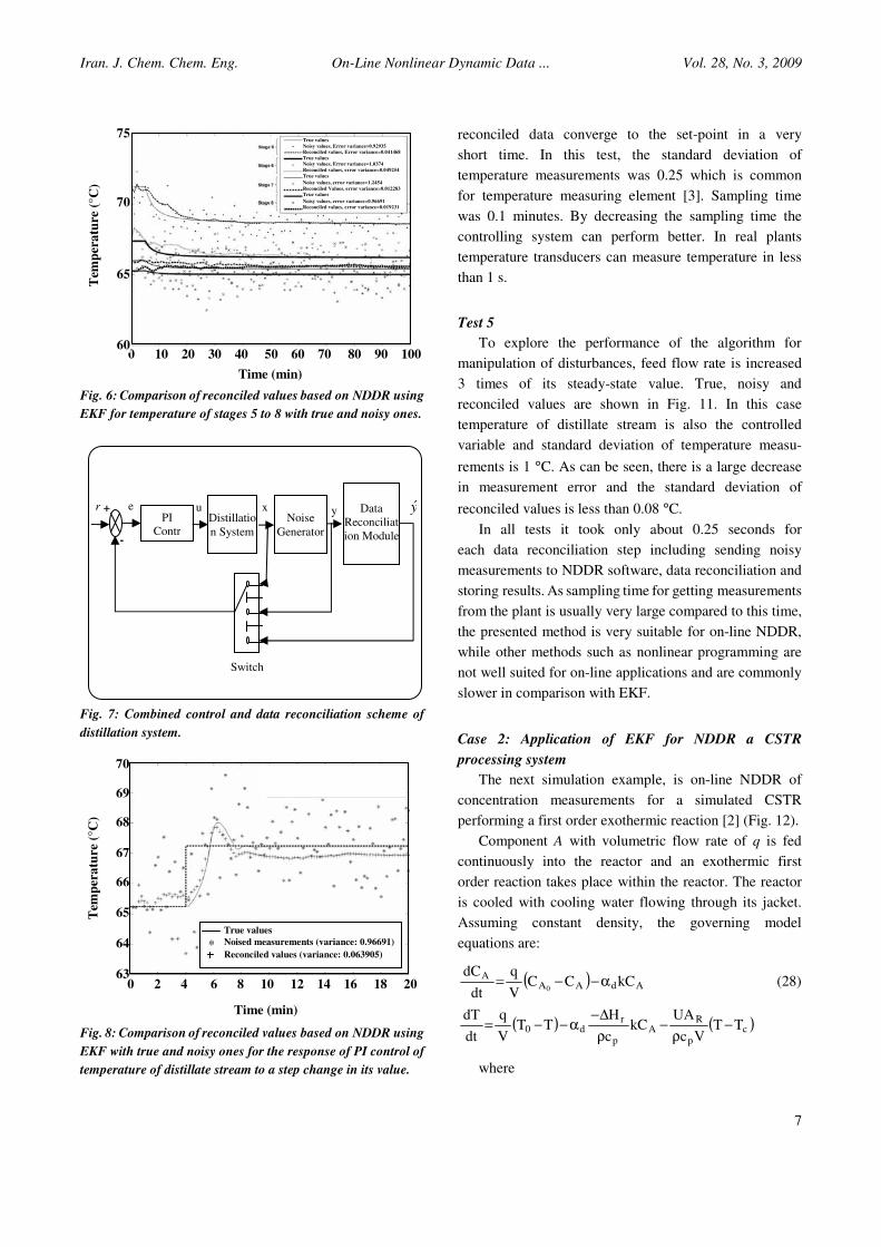
Test 3

The above results were performed for open-loop

system. To show the performance of the system

in closed-loop case, a combined control and data

reconciliation scheme is defined (Fig. 7). A switching

element is used between true and reconciled values in

order investigate their effect on controller performance.

Temperature of distillate stream is selected as

controlled variable, and reflux ratio as manipulating one.

The response of the system to a step change of +2 °C in

the set-point of controlled variable using a PI controller is

obtained. The controller parameters are adjusted based on

classic Ziegler-Nichols method. The results of reconciled,

true and noisy values are depicted in Fig. 8. The standard

deviation of added white noises to true temperature

values in this case is set to 1 °C. As can be seen, however

the reconciled values show a fair set-point tracking, and

have standard deviation of 0.25.

Test 4

In the above test, controller input was the true values

generated by the simulation. In real plants true data are

not available and only noisy measurements are used for

control. But the use of these noisy data has a bad

influence on the performance of the controlling system.

To investigate the impact of using noisy or reconciled

values on controller performance, firstly noisy data and

then reconciled values are used for the control of

distillation column.

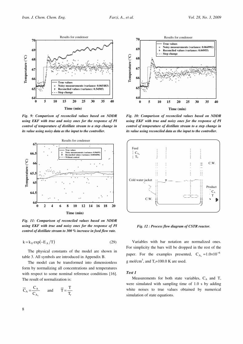
As it can be seen from Figs. 9 and 10, using noisy

values causes the divergence of reconciliation process

and the temperature of distillate stream oscillates

continuously while using reconciled values avoids

oscillation, causes the distillate temperature to reach to

its set-point value after a relatively long time while

NDDR

Module

Simulator

Real Plant

Simulated measured

(noisy) data via

DDE/COM/DLL

Real measured

(noisy) data via

Serial/Parallel Ports

Reconciled data

(for various

applications)

0 40 80 120 160 200 240

Time (min)

100

96

92

88

84

80

76

72

68

64

Tem

per

atu

re (

°C)

0 50 100 150

Time (min)

84

82

80

78

76

74

73

70

68

Tem

per

atu

re (

°C)

Tray ≠1

Tray ≠2

Feed plateTray ≠4

Tray ≠5

Tray ≠6

Exit from condenser

Reboiler

True values

Noised measurements (variance: 1.1371)

Reconciled values (variance: 0.020413) *


7

Fig. 6: Comparison of reconciled values based on NDDR using

EKF for temperature of stages 5 to 8 with true and noisy ones.

Fig. 7: Combined control and data reconciliation scheme of

distillation system.

Fig. 8: Comparison of reconciled values based on NDDR using

EKF with true and noisy ones for the response of PI control of

temperature of distillate stream to a step change in its value.

reconciled data converge to the set-point in a very

short time. In this test, the standard deviation of

temperature measurements was 0.25 which is common

for temperature measuring element [3]. Sampling time

was 0.1 minutes. By decreasing the sampling time the

controlling system can perform better. In real plants

temperature transducers can measure temperature in less

than 1 s.

Test 5

To explore the performance of the algorithm for

manipulation of disturbances, feed flow rate is increased

3 times of its steady-state value. True, noisy and

reconciled values are shown in Fig. 11. In this case

temperature of distillate stream is also the controlled

variable and standard deviation of temperature measu-

rements is 1 °C. As can be seen, there is a large decrease

in measurement error and the standard deviation of

reconciled values is less than 0.08 °C.

In all tests it took only about 0.25 seconds for

each data reconciliation step including sending noisy

measurements to NDDR software, data reconciliation and

storing results. As sampling time for getting measurements

from the plant is usually very large compared to this time,

the presented method is very suitable for on-line NDDR,

while other methods such as nonlinear programming are

not well suited for on-line applications and are commonly

slower in comparison with EKF.

Case 2: Application of EKF for NDDR a CSTR

processing system

The next simulation example, is on-line NDDR of

concentration measurements for a simulated CSTR

performing a first order exothermic reaction [2] (Fig. 12).

Component A with volumetric flow rate of q is fed

continuously into the reactor and an exothermic first

order reaction takes place within the reactor. The reactor

is cooled with cooling water flowing through its jacket.

Assuming constant density, the governing model

equations are:

( ) AdAAA

kCCCV

q

dt

dC0

α−−= (28)

( ) ( )cp

RA

p

rd0 TT

Vc

UAkC

c

HTT

V

q

dt

dT−

ρ−

ρ

Δ−α−−=

where

u eDistillatio

n System-

r xPI

Contr

+ Data

Reconciliat

ion Module

Switch

Noise

Generator

yy

0 10 20 30 40 50 60 70 80 90 100

Time (min)

75

70

65

60

Tem

per

atu

re (

°C)

0 2 4 6 8 10 12 14 16 18 20

Time (min)

70

69

68

67

66

65

64

63

Tem

per

atu

re (

°C)

True values

Noisy values, Error variance=0.92935

Reconciled values, Error variance=0.041468

True values

Noisy values, Error variance=1.0374

Reconciled values, error variance=0.049254

True values

Noisy values, error variance=1.2454

Reconciled Values, error variance=0.012283

True values

Noisy values, error variance=0.96691

Reconciled values, error variance=0.019231

True values


Reconciled values (variance: 0.063905) *


8


using EKF with true and noisy ones for the response of PI

control of temperature of distillate stream to a step change in

its value using noisy data as the input to the controller.



control of distillate stream to 300 % increase in feed flow rate.

( )TEexpkk A0 −= (29)

The physical constants of the model are shown in

table 3. All symbols are introduced in Appendix B.

The model can be transformed into dimensionless

form by normalizing all concentrations and temperatures

with respect to some nominal reference conditions [16].

The result of normalization is:

rA

AA

T

TTand

C

CC

r

==



control of temperature of distillate stream to a step change in

its value using reconciled data as the input to the controller.

Fig. 12 : Process flow diagram of CSTR reactor.

Variables with bar notation are normalized ones.

For simplicity the bars will be dropped in the rest of the

paper. For the examples presented, 6A 100.1C

r

−×=

g mol/cm3, and Tr=100.0 K are used.

Test 1

Measurements for both state variables, CA and T,

were simulated with sampling time of 1.0 s by adding

white noises to true values obtained by numerical

simulation of state equations.

0 5 10 15 20 25 30 35 40

Time (min)

70

69

68

67

66

65

64

Tem

per

atu

re (

°C)

Results for condenser

0 5 10 15 20 25 30 35 40

Time (min)

70

69

68

67

66

65

64

Tem

per

atu

re (

°C)


0 2 4 6 8 10 12 14 16 18 20

Time (min)

67

66.5

66

65.5

65

64.5

64

Tem

per

atu

re (

°C)


C.W.

Feed

Product

Cold water jacket

C.W.

CA0

T0

CA

T

True values

Noisy measurements (variance: 0.065483)

Reconciled values (variance: 0.54505)

Step change

*

True values



Without control

*

True values



Step change

*


9

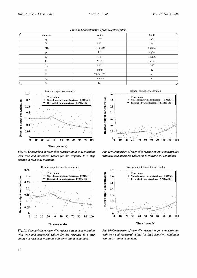
The simulation initialized at a steady-state condition

of 5.6C0A = , 5.3T0 = , 1531.0CA = and T=4.6091. A

step change of 6.5 to 7.5 in feed concentration was

performed at t = 30 s. The method of EKF was applied on

noisy measurements. The reconciled, true and noisy

measurements with respect totime are shown in Fig. 13.

The estimated values contain a lower level noise in

comparison with the simulated measurements. As shown,

the reconciled data follow the true values very closely.

The standard deviation of errors in reconciled values is

0.0013 which is 38 times smaller than standard deviation

of errors in measurements (0.05).

In reality, steady-state values of CA and T, i.e. initial

conditions for Eq. (30), are also measured and may

contain some errors. In order to see the effect of

uncertainty in steady state measurements, random noises

with the same standard deviation have been added into

the simulated steady-state and dynamic results and the

performance of EKF method is checked.

As shown in Fig. 14, the fitness of reconciled values

with true ones is very good. They have a standard

deviation of 0.0052 which is much lower than 0.05 for

noisy measurements.

Test 2

To show the benefits of EKF in highly transient

behavior of the system a more challenging test was

performed by beginning the simulation in a transient state.

The feed temperature T0 was held constant at 4.6091 and

the feed concentration was sequentially stepped from 7.5

to 8.5 at time 40s and to 5.5 at time 60s. The reconciled

values of CSTR measurements were significantly

smoother than the simulated measurements (Fig. 15).

( ) AdAAA

CkCCV

q

dt

Cd0

α−−= (30)

( ) ( )cp

RA

rp

Ard0 TT

Vc

UACk

Tc

CHTT

V

q

dt

Tdr −

ρ−

ρ

Δα−−=

��

��

� −=

r

A0

TT

Eexpkk

where

The standard deviation of the results is 0.0034. By

introducing noises to initial conditions, the standard

deviation of the results becomes 0.0076 (Fig. 16).

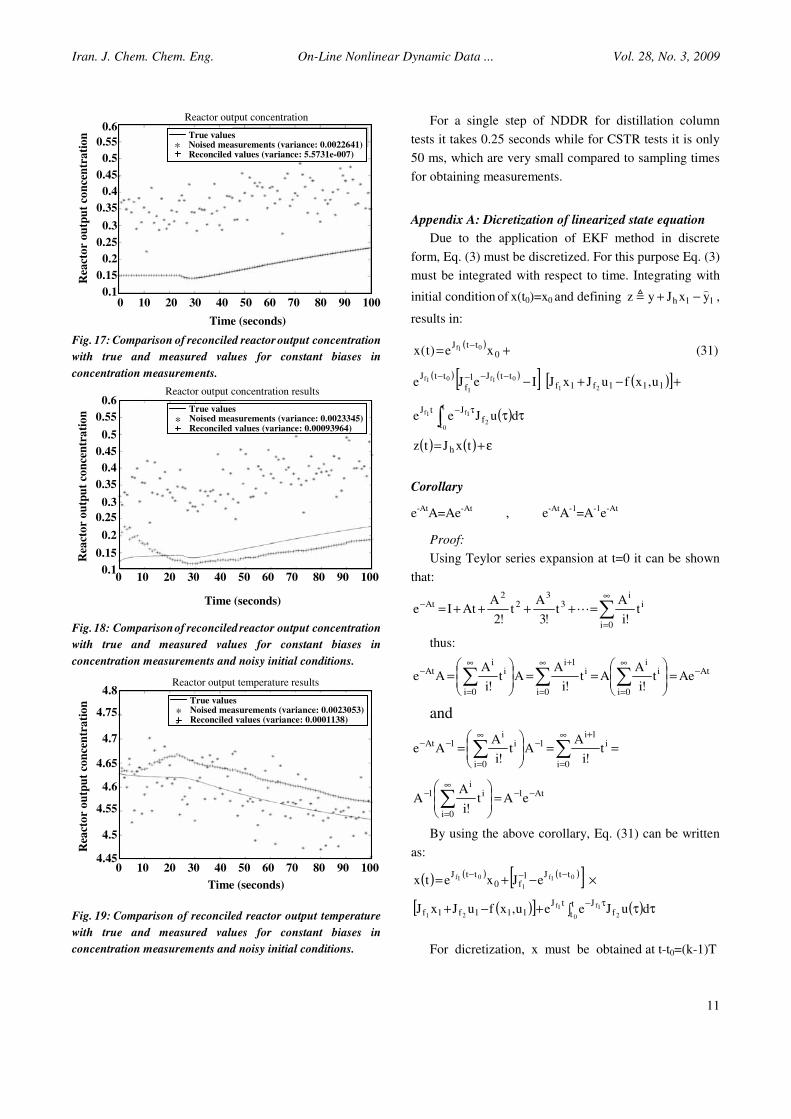
Test 3

To evaluate the ability of the algorithm to deal with

biases, a test was performed. The bias is defined as the

mean value of the measurements. A constant bias of 0.2

was added to all concentration measurements. A step

change from 6.5 to 6.0 was performed on feed

concentration at t = 25 s. Fig. 17 shows the results which

completely fit true values. But by introducing random

noises into initial conditions, the mean value of results

becomes nonzero, however this mean value (-0.0166) is

very small compared to the mean value of noises (0.2)

(Fig. 18).

To show the effect of reconciliation of unbiased

measurements when biases in some other measurements

exist, the results for temperature measurements

reconciliation for the last case are also shown in Fig. 19.

As it is evident, reconciled values have a bias with mean

value of 0.037 while noisy temperature measurements do

not contain any biases. Computation time for all reactor

tests was about 50 ms in each single step of NDDR

using EKF.

CONCLUSIONS

The advantages of EKF algorithm for on-line

nonlinear dynamic data reconciliation are presented. It is

used for NDDR of a two-component distillation column

and a CSTR. Different tests are performed for two cases

to show the performance of EKF method for on-line

NDDR. Results show considerable decrease in

measurement errors. Results of the application of EKF

show a high performance even for highly nonlinear

systems. Also in the case of existence of noises in initial

conditions, the reconciled values based on the application

of EKF are converged to the true values after a short time

since the start of the run by removing noises.

When measurements contain constant biases, the filter

successfully removes noises from measurements, but it

introduces a very small bias to reconciled values compared

to the original bias. This is due to the formulation of EKF

that no penalties have been considered for biases. Thus, it

will be more convenient to apply a gross error detection

algorithm before applying EKF.

The other main advantage of this algorithm is that it is

very fast for performing a single step of NDDR. This

method can reconciliate measurements very quickly.


10

Table 3: Characteristics of the selected system.

Parameter Value Units

q 10-5 m3/s

V 0.001 m3

-ΔHr -1.130×108 J/kgmol

ρ 1.0 Kg/m3

cp 4184 J/kg.K

U 20.92 J/m2.s.K

AR 0.001 M2

Tc 340.0 K

K0 7.86×1012 s-1

EA 14090.0 K

αd 1.0 ⎯

Fig. 13: Comparison of reconciled reactor output concentration

with true and measured values for the response to a step

change in feed concentration.


with true and measured values for the response to a step

change in feed concentration with noisy initial conditions.


with true and measured values for high transient conditions.


with true and measured values for high transient conditions

whit noisy initial conditions.

Reactor output concentration results

0 10 20 30 40 50 60 70 80 90 100

Time (seconds)

0.35

0.3

0.25

0.2

0.15

0.1

0.05

0

Rea

cto

r o

utp

ut

con

cen

tra

tio

n

Reactor output concentration

0 10 20 30 40 50 60 70 80 90 100

Time (seconds)

0.35

0.3

0.25

0.2

0.15

0.1

0.05

0

Rea

cto

r o

utp

ut

con

cen

tra

tio

n

0 10 20 30 40 50 60 70 80 90 100

0.7

0.6

0.5

0.4

0.3

0.2

0.1

0

Rea

cto

r o

utp

ut

con

cen

tra

tio

n


0 10 20 30 40 50 60 70 80 90 100

Time (seconds)

0.7

0.6

0.5

0.4

0.3

0.2

0.1

0

Rea

cto

r o

utp

ut

con

cen

tra

tio

n


True values


Reconciled values (variance: 1.5722e-006) *

True values



True values



True values




11


with true and measured values for constant biases in

concentration measurements.

Fig. 18: Comparisonof reconciled reactor output concentration


concentration measurements and noisy initial conditions.

Fig. 19: Comparison of reconciled reactor output temperature


concentration measurements and noisy initial conditions.

For a single step of NDDR for distillation column

tests it takes 0.25 seconds while for CSTR tests it is only

50 ms, which are very small compared to sampling times

for obtaining measurements.

Appendix A: Dicretization of linearized state equation

Due to the application of EKF method in discrete

form, Eq. (3) must be discretized. For this purpose Eq. (3)

must be integrated with respect to time. Integrating with

initial condition of x(t0)=x0 and defining h 1 1z y J x y+ −�� ,

results in:

( )+=

−0

ttJxe)t(x 01f (31)

( ) ( )[ ] ( )[ ]+−+−−−−−

111f1fttJ1

f

ttJu,xfuJxJIeJe

21

01f

1

01f

( )� τττ−t

tf

JtJ

02

1f1f duJee

( ) ( ) ε+= txJtz h

Corollary

e-At

A=Ae-At

, e-At

A-1

=A-1

e-At

Proof:

Using Teylor series expansion at t=0 it can be shown

that:

�∞

=

− =++++=0i

ii

33

22

At t!i

At

!3

At

!2

AAtIe �

thus:

At

0i

ii

0i

i1i

0i

ii

AtAet

!i

AAt

!i

AAt

!i

AAe

−∞

=

∞

=

+∞

=

− =��

��

�==�

��

��

�= ��

and

==��

��

�= ��

∞

=

+−

∞

=

−−

0i

i1i

1

0i

ii

1Att

!i

AAt

!i

AAe

At1

0i

ii

1eAt

!i

AA

−−∞

=

− =��

��

��

By using the above corollary, Eq. (31) can be written

as:

( ) ( ) ( )[ ] ×−+=−−− 01f

1

01fttJ1

f0ttJ

eJxetx

( )[ ] ( )� ττ+−+τ−t

t fJtJ

111f1f0 2

1f1f

21duJeeu,xfuJxJ

For dicretization, x must be obtained at t-t0=(k-1)T

0 10 20 30 40 50 60 70 80 90 100

Time (seconds)

0.6

0.55

0.5

0.45

0.4

0.35

0.3

0.25

0.2

0.15

0.1

Rea

cto

r o

utp

ut

con

cen

tra

tio

n


0 10 20 30 40 50 60 70 80 90 100

Time (seconds)

0.6

0.55

0.5

0.45

0.4

0.35

0.3

0.25

0.2

0.15

0.1

Rea

cto

r o

utp

ut

con

cen

tra

tio

n


0 10 20 30 40 50 60 70 80 90 100

Time (seconds)

4.8

4.75

4.7

4.65

4.6

4.55

4.5

4.45

Rea

cto

r o

utp

ut

con

cen

tra

tio

n

Reactor output temperature results

True valuesNoised measurements (variance: 0.0022641) Reconciled values (variance: 5.5731e-007)

*

True valuesNoised measurements (variance: 0.0023345) Reconciled values (variance: 0.00093964)

*

True valuesNoised measurements (variance: 0.0023053) Reconciled values (variance: 0.0001138)

*


12

and t-t0=kT. Assuming that 1f

J , x1, 2fJ , u and f(x1,u1) are

constant within this time domain, it can be shown that:

( )[ ] ( ) ( )[ ]×−+=− −−− T1k1f

1

1fJ1

f0T1kJ

eJxeT1kx

( )[ ] ( )[ ]{ } ( )[ ]T1kuJIeJu,xfJxJ2

01f

121 ftT1kJ1

f11f1f −−+−+−−−

( ) [ ] ( )[ ]+−+−+= −111f1f

KTJ1f0

kTf u,xfuJxJeJxekTx21

f1

[ ]{ } =−−− uJIeJ

2

01f

1 ftkTJ1

f

( ) ( )[ ]{ T1kJ1f

TJ0

T1kJTJ1f

1

1f1f1f eJexee−−−−

−+

( )[ ]+−+ 111f1f u,xfuJxJ21

[ ]{ } ( )[ ]}=−− −−−− T1kuJeeJ2

f01f

1 fTJtT1kJ1

f

( )[ ]{ +− T1kxeTJ

1f

( )[ ] ( )[ ]+−+−−−

111f1fT1kJ1

fTJ

u,xfuJxJeJE21

1f

1

1f

( )[ ]{ } ( )[ ]−−− −−−T1kuJeeJ

2

f01f

1 fTJtT1kJ1

f

( )[ ] ( )[ ]−−+−−−

111f1fT1kJ1

f u,xfuJxJeJ21

1f

1

( )[ ]{ } ( )[ ]}=−−−−− T1kuJIeJ

2

02f

1 ftT1kJ1

f

( )[ ]{ +− T1kxeTJ

2f

[ ] ( )[ ]+−+− −−−111f1f

1f

1f

TJu,xfuJxJJJe

2111

1f

[ ] ( )[ ]}=−−−− T1kuJeIJ

2

1f

1 fTJ1

f

( )[ ]+− T1kxeTJ

1f

[ ] ( )[ ]+−+− −−111f1f

1f

TJ1f u,xfuJxJJeJ

211

1f

[ ] ( )[ ]=−− −− T1kuJJJe211

1f

f1

f1

fTJ

( )[ ]+− T1kxeTJ

1f

( ) ( )[ ]+−+− −111f1f

1TJu,xfuJxJJeI

211f

2f

( ) ( )[ ]=−− − T1kuJJIe21

1f

f1

fTJ

( )[ ] ( )×−+−TJTJ

1f1f eIT1kxe

( )[ ]( ) ( )[ ]111

f1f1

f1 u,xfJT1kuuJJx121

−− −−−+

Where in discrete form it can be written as:

[ ] [ ] [ ] M1kuB1kxAkx +−⋅+−⋅= (32)

[ ] [ ] ε+= kxJkz h

( )21

1f

f1

fTJ

JJIAB,eA −−==

( ) ( )[ ] 1111

f1 Buu,xfJxAIM1

−−−= −

APPENDIX B: LIST OF SYMBOLS

1- List of used symbols in mathematical model of

distillation column

Symbols

Dn Product flow rate from stage n (g mol/min)

En Murphree efficiency for stage n

Fn Feed flow rate to stage n (g mol/min)

Gk,I Interaction parameter between components

k and i, Eq. (16)

hf,n Enthalpy of feed stream entering stage n (J/g mol)

Ki K-value of component i at system

temperature and pressure

Ki,n K-value of component i on stage n

Ln Liquid a flow rate on stage n (g mol/min)

Mc,n Heat capacity of stage n (J/K)

m Total number of components = 2

P Total pressure (Pa)

Pi* Vapor pressure of component i at system

temperature (Pa)

Qc,n Heat entered to stage n (J/min)

qc,n Heat loss from stage n (J/min)

SL,I Liquid heat capacity of component i (J/g mol.K)

SV,I Vapor heat capacity of component i (J/g mol.K)

T System temperature (K)

Tn Temperature on stage n (K)

t Time (min)

Vn Gas flow rate on stage n (g mol/min)

νLn Liquid hold-up on stage n (m3)

νVn Gas hold-up on stage n (m3)

xi Molar composition of component i in liquid phase

xi,n Molar composition of component i in

liquid stream on stage n

xi,n (e) Molar composition of

component i in liquid phase in equilibrium with

yi,n at system temperature and pressure on stage n

xf,n Molar composition of methanol in feed

stream entering to stage n

yi Molar composition of component i in vapor phase

yi,n Molar composition of component i

in vapor stream on stage n

Greek Symbol

γi Activity coefficient of component i at

system temperature

λI Heat of vaporization of component i (J/ g mol)

ρLn, ρVn Liquid and vapor molar density on stage n,

respectively (g mol /m3)


13

Subscripts

i, j, k Component indices

n Stage index

2- List of used symbols in mathematical model of CSTR

Symbols

AR Cross section of reactor tank (m2)

CA Concentration of reactor content (kg mol/m3)

0AC Concentration of component A in feed (kg mol/m3)

rAC Reference value of reactant concentration =

1.0×10-3

kg mol/m3

AC Normalized concentration )C/C(rAA

cp Heat capacity of reactor content (J/kg.K)

EA Activation energy of the reaction (K)

ΔHR Heat of reaction

k Reaction rate constant (s-1

)

k0 Constant coefficient in Arhenius equation

q Feed flow rate (m3/s)

T Temperature of reactor content (K)

T0 Feed temperature (K)

Tc Temperature of cooling water (K)

Tr Reference value of temperature = 100 K

T Normalized temperature (T/Tr)

U Overall heat transfer coefficient

between reactor content and jacket (W/m2.K)

V Volume of reactor content (m3)

Greek Symbols

αd Catalyst deactivation constant (dimensionless)

ρ Density of reactor content (kg/m3)

Received : 28th February 2008 ; Accepted : 24th February 2009

REFRENCES

[1] Almasy, G. A., Principles of Dynamic Balancing,

AIChE Journal, 36, p. 1321 (1991).

[2] Liebman, M. J., Edgar, T. F. and Lasdon, L. S.,

Efficient Data Reconciliation and Estimation for

Dynamic Processes using Nonlinear Programming

Techniques, Computers Chem. Engng., 16 (10/11),

p. 963 (1992).

[3] Bai, S., Thibault, J. and McLean, D. D., Dynamic

Data Reconciliation: Alternative to Kalman Filter,

Journal of Process Control, 16 (9), p. 938 (2006).

[4] Abu-el-zeet, Z. H., Becerra, V.M., Roberts, P.D.,

Combined Bias and Outlier Identification in

Dynamic Data Reconciliation, Computers Chem.

Engng., 26, p. 921 (2002).

[5] Barbosa Jr, V. P., Wolf, M. R. M., Maciel Fo, R.,

Development of Data Reconciliation for Dynamic

Nonlinear System: Application to the Polymerization

Reactor, Computers Chem. Engng., 24, p. 501

(2000).

[6] McBrayer, K. F., Soderstorm, T. A., Edgar, T. F. and

Young, R. E., The Application of Nonlinear

Dynamic Data Reconciliation to Plant Data,

Computers Chem. Engng., 22 (12), p. 1907 (1998).

[7] Meert, K., A Real-Time Recurrent Learning Network

Structure for Data Reconciliation, Artificial

Intelligence in Engineering, 12, p. 213 (1998).

[8] Chen, J., Romagnoli, J. A., A Strategy for Simul-

taneous Dynamic Data Reconciliation and Outlier

Detection, Computers Chem. Engng., 22 (4/5), p.

559 (1998).

[9] Karjala, T. W., Himmelblau, D. M., Dynamic

Rectification of Data via Recurrent Neural Network

and the Extended Kalman Filter, AIChE Journal,

42, p. 2225 (1996).

[10] Islam, K. A., Weiss, G. H. and Romagnoli, J. A.,

Nonlinear Data Reconciliation for an Industrial

Pyrolysis Reactor, 4th

European Symposium on

Computer Aided Process Engineering, p. 218

(1994).

[11] Chiari, M., Bussani, G., Grottoli, M. G. and

Pierucci, S., On-Line Data Reconciliation and

Optimization: Refinery Applications, 7th

European

Symposium on Computer Aided Process Engineering,

p. 1185 (1997).

[12] Grewal, M. S. and Andrews, A. P., “Kalman

Filtering: Theory and Practice Using MATLAB”,

Second Edition, John Wiley and Sons Inc., (2001).

[13] Narasimhan, S. and Jordache, C., “Data Recon-

ciliation and Gross Error Detection: An Intelligent

Use of Process Data”, Gulf Professional Publishing,

Houston, Texas, Nov. (1999).

[14] Mehrabni, A. Z., “Non-linear Parameter Estimation

of Distillation Column”, M.Sc. Thesis, University of

Wales, Department of Chemical Engineering, Nov.

(1986).


14

[15] Farzi, A., Mehrabani, A.Z. and Bozorgmehry, R. B.,

Data Reconciliation: Development of an Object-

Oriented Software Tool, Korean Journal of

Chemical Engineering, 25 (5), p. 955 (2008).

[16] Jang, S. S., Joseph, B. and Mukai, H., Comparison

of Two Approaches to On-Line Parameter and State

Estimation of Nonlinear Systems, Ind. Engng.

Chem. Process. Des. Dev., 25, p. 809 (1986).

Documents

On-Line Nonlinear Dynamic Data Reconciliation Using Extended Kalman Filtering ...€¦ · · 2018-02-20Iran. J. Chem. Chem. Eng. Vol. 28, No. 3, 2009 1 On-Line Nonlinear Dynamic