Embed Size (px)
Citation preview

ON-LINE NEW EVENT DETECTION AND CLUSTERING USING THE CONCEPTS OF THE COVER COEFFICIENT-BASED CLUSTERING
METHODOLOGY
A THESIS
SUBMITTED TO THE DEPARTMENT OF COMPUTER
ENGINEERING
AND THE INSTITUTE OF ENGINEERING AND SCIENCE
OF BILKENT UNIVERSITY
IN PARTIAL FULLFILLMENT OF THE REQUIREMENTS
FOR THE DEGREE OF
MASTER OF SCIENCE
by
Ahmet Vural
August, 2002

ii
I certify that I have read this thesis and that in my opinion it is fully adequate, in
scope and in quality, as a thesis for the degree of Master of Science.
Prof. Dr. Fazlı Can ( Advisor )
I certify that I have read this thesis and that in my opinion it is fully adequate, in
scope and in quality, as a thesis for the degree of Master of Science.
Asst. Prof. Dr. Uğur Güdükbay
I certify that I have read this thesis and that in my opinion it is fully adequate, in
scope and in quality, as a thesis for the degree of Master of Science.
Assoc. Prof. Dr. Özgür Ulusoy
Approved for the Institute of Engineering and Science:
Prof. Dr. Mehmet B. Baray
Director of Institute of Engineering and Science

iii
ABSTRACT
ONLINE NEW EVENT DETECTION AND CLUSTERING USING THE CONCEPTS OF THE COVER COEFFICIENT-BASED CLUSTERING
METHODOLOGY
Ahmet Vural M.S. in Computer Engineering
Supervisor: Prof. Dr. Fazlı Can August, 2002
In this study, we use the concepts of the cover coefficient-based clustering
methodology (C3M) for on-line new event detection and event clustering. The
main idea of the study is to use the seed selection process of the C3M algorithm
for the purpose of detecting new events. Since C3M works in a retrospective
manner, we modify the algorithm to work in an on-line environment.
Furthermore, in order to prevent producing oversized event clusters, and to give
equal chance to all documents to be the seed of a new event, we employ the
window size concept. Since we desire to control the number of seed documents,
we introduce a threshold concept to the event clustering algorithm. We also use
the threshold concept, with a little modification, in the on-line event detection. In
the experiments we use TDT1 corpus, which is also used in the original topic
detection and tracking study. In event clustering and event detection, we use both
binary and weighted versions of TDT1 corpus. With the binary implementation,
we obtain better results. When we compare our on-line event detection results to
the results of UMASS approach, we obtain better performance in terms of false
alarm rates.
Keywords: Clustering, on-line event clustering, on-line event detection.
iv
ÖZET
KAPLAMA KATSAYISI TABANLI KÜME OLUŞTURMA METODOLOJİSİ KULLANARAK ANINDA YENİ OLAY BELİRLEME VE KÜME
OLUŞTURMA
Ahmet Vural Bilgisayar Mühendisliği, Yüksek Lisans
Tez Yöneticisi: Prof. Dr. Fazlı Can Ağustos, 2002
Bu çalışmada, anında yeni olay belirlemek ve olay kümeleri oluşturmak amacıyla,
kaplama katsayısı tabanlı küme oluşturma metodolojisi (C3M) kavramları
kullanıldı. Çalışmanın ana teması, yeni olay belirlemek için C3M algoritmasının
tohum seçme işlemini kullanmaktır. C3M’in çalışma prensibi anında kümelemeye
uygun olmadığından, algoritmada değişiklikler yapıldı. Ayrıca, çok büyük olay
kümelerinin oluşumunu önlemek ve bütün dokümanlara, tohum olabilmeleri için
eşit şans tanımak amacıyla, pencere yöntemi kullanıldı. Tohum dokümanlarının
miktarını kontrol etmek maksadıyla, olay kümeleme işi için bir eşik kavramı
ortaya çıkarıldı. Bu kavramı, çok küçük değişikliklerle, yeni olay belirlemede de
kullanıldı. Deneyler esnasında, orjinal konu belirleme ve takip çalışmasında da
kullanılan TDT1 yığınından yararlanılmıştır. Yeni olay belirleme ve olay
kümeleme işlemlerinde TDT1 yığınının ağırlıklı ve düz uyarlamaları kullanıldı.
Düz uygulamalar için daha iyi sonuçlar elde edildi. Anında olay belirleme
alanındaki sonuçlar UMASS yaklaşımınınkilerle karşılaştırıldığında, yanlış alarm
oranları açısından daha iyi performans elde edilmiştir.
Anahtar Sözcükler: Kümeleme, anında olay kümelemesi, anında olay belirleme.

v
ACKNOWLEDGEMENTS
I would like to express my special thanks and gratitude to Prof. Dr. Fazlı
Can, from whom I have learned a lot, due to his supervision, suggestions, and
support during this research.
I am also indebted to Assoc. Prof. Dr. Özgür Ulusoy and Assist. Prof. Dr.
Uğur Güdükbay for showing keen interest to the subject matter and accepting to
read and review this thesis.
I would like to thank to Turkish Armed Forces for giving this great
opportunity.
I would like to thank all my colleagues and dear friends for their help and
support.

vi
Anneme ve Ablalarıma.

vii
Contents
1 Introduction ....................................................................................................1
1.1 Definitions ..................................................................................................1
1.2 Research Contributions ...............................................................................3
1.3 Thesis Overview .........................................................................................4
2 Related Work ..................................................................................................5
2.1 New Event Detection Approaches ...............................................................6
2.1.1 CMU Approach..................................................................................7
2.1.2 The UMass Approach.........................................................................8
2.1.3 Dragon System Approach...................................................................9
2.1.4 UPenn Approach .............................................................................. 10
2.1.5 BBN Technologies' Approach .......................................................... 10
2.1.6 On-Line New Event Detection in a Multi-Resource Environment..... 11
2.2 Event Clustering Approaches .................................................................... 12
2.3 Document Clustering Approaches ............................................................. 14
2.3.2 Single-Pass Clustering...................................................................... 15
2.3.3 Cover Coefficient-based Clustering Methodology ............................ 16
3 Cover Coefficient-based Clustering Methodology: C3M............................. 17
4 Experimental Data and Evaluation Methods............................................... 24

viii
4.1 TDT Corpus.............................................................................................. 24
4.2 Evaluation................................................................................................. 26
4.2.1 Effectiveness Measures .................................................................... 26
4.2.1 Experimental Methodology .............................................................. 29
4.2.2 Preprocessing ................................................................................... 29
5 On-Line Event Clustering............................................................................. 31
5.1 Window Size............................................................................................. 31
5.2 Threshold Model....................................................................................... 34
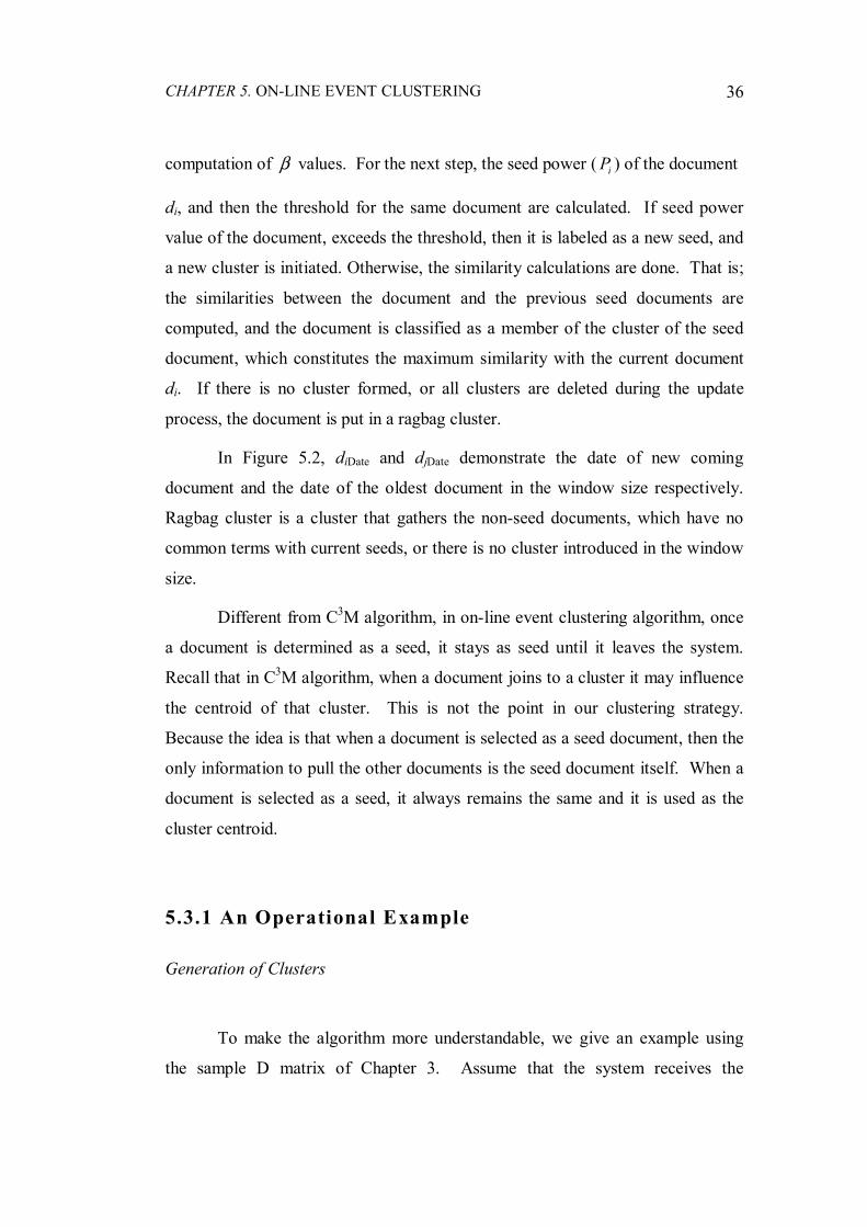
5.3 The Algorithm .......................................................................................... 35
5.3.1 An Operational Example .................................................................. 36
5.4 Experimental Results ................................................................................ 40
5.4.1 Results of Binary Implementation .................................................... 40
5.4.2 Results of Weighted Implementation................................................ 42
6 On-Line New Event Detection ...................................................................... 46
6.1 Window Size............................................................................................. 46
6.2 Threshold Model....................................................................................... 47
6.3 The Algorithm .......................................................................................... 48
6.3.1 An Operational Example .................................................................. 49
6.4 Experimental Results ................................................................................ 51
6.4.1 Results of Binary Implementation .................................................... 51
6.4.2 Results of Weighted Implementation................................................ 53
7 Conclusion and Future Work....................................................................... 57

ix
List of Figures
1.1 On-line new event detection, event tracking, event clustering and ..........2
2.1 Single-pass clustering algorithm.............................................................8
2.2 UMASS new event detection algorithm. ................................................9
2.3 BBN new event detection algorithm. .................................................... 11
2.4 New event detection and tracking algorithm......................................... 11
3.1 C3M Algorithm. ................................................................................... 18
3.2 Sample D Matrix.................................................................................. 18
3.3 S and TS ′ matrixes derived from the D matrix of Figure 3.2. ............... 20
3.4 Sample C matrix .................................................................................. 20
3.5 Some properties of the C matrix. .......................................................... 22
4.1 Judged 25 events in TDT corpus. ......................................................... 25
4.2 An example document vector. .............................................................. 30
5.1 Event evolution; Oklahoma city bombing ............................................ 33
5.2 On-line event clustering algorithm. ...................................................... 35
5.3 Final event clusters. ............................................................................. 38
5.4 Effectiveness measure results for the example data. ............................. 39
5.5 Change of effectiveness measures vs. window size (binary). ................ 41

x
5.6 Change of performance (pfr)vs. window size. ...................................... 42
5.7 Change of effectiveness measures vs. window size (weighted)............. 43
5.8 Change of performance (pfr) vs. window size. ..................................... 44
5.9 Comparison of effectiveness measures (recall, precision, F1, miss). ..... 45
5.10 Comparison of implementation performances (pfr). ............................. 45
6.1 On-line new event detection algorithm. ................................................ 48
6.2 Effectiveness measure results for the example data. ............................. 50
6.3 Change of effectiveness measures vs. window size. ............................. 52
6.4 Change of performance vs. window size. ............................................. 52
6.5 Change of effectiveness measures vs. window size. ............................. 54
6.6 Change of performance vs. window size. ............................................. 54
6.7 Comparison of effectiveness measures (recall, precision, F1, miss). ..... 55
6.8 Comparison of implementation performances.(pfr) .............................. 55

xi
List of Tables
2.1 The summary of on-line new event detection approaches ...................... 12
4.1 Two-by-two contingency table for event clustering. .............................. 27
4.2 Two-by-two contingency table for event detection. ............................... 28
5.1 Distribution of the documents in time (window size in days)................. 32
5.2 Event clustering results according to six window sizes (binary)............. 40
5.3 Event clustering results according to six window sizes (weighted). ....... 43
6.1 Final document labels. .......................................................................... 50
6.2 On-line event detection results according to four windows (binary)....... 51
6.3 On-line new event detection results according to four windows............. 53
6.4 Comparison of on-line new event detection approaches. ....................... 56
6.5 Comparison of systems presented at the first TDT workshop. ............... 56

xii
List of Symbols and Abbreviations
iα : Alpha, reverse of row sum of D matrix.
kβ : Beta, reverse of column sum of D matrix.
iδ : Decoupling coefficient.
iψ : Coupling coefficient.
iP : Cluster seed power of document di.
P : Average seed power value.
C : Document-by-document (m × m) cover coefficient matrix whose
entries, cij values, indicate the probability of selecting any term of
document (di) from document (dj), where di and dj are the
members of D matrix.
C ′ : Term-by-term (n × n) cover coefficient matrix.
C3M : Cover Coefficient based Clustering Methodology .
CBR : Cluster-Based Retrieval.
CC : Cover Coefficient.
cij : The probability of selecting any term of di from dj..
CMU : Carnegie Mellon University.
D : Document–by-term matrix, contains document vectors.
diDate : The date of new coming document.
djDate : The date of the oldest document in the current window.
DRAGON : Dragon Systems.
FS : Full Search.
JGI : Journal of Graphics Institute.

xiii
KNN : k Nearest Neighbour Algorithm.
LDC : Linguistic Data Consortium.
m : The number of documents in the database.
MUC : Message Understanding Conferences.
TDT : Topic Detection and Tracking.
tf× idf : Term Frequency times Inverse Document Frequency.
tgs : The average number of seed documents per term.
Tr : Threshold value.
UMASS : University of Massachusetts at Amherst.
WS : Window Size.
xd : The average number of distinct terms per document.

1
Chapter 1 Introduction 1.1 Definitions
We live in a quickly changing world. We do not have time to stop and rest for a
moment, if we do not want to miss the developments in the changing world. How
much can human being resist this stress? There should be a way to save our time
and our life. The computer can help, but it is not enough. In addition to
computer, an intelligent assistant system is desirable. This system should be able
to follow the current news, form of a content summary of a corpus for a quick
review, provide a temporal evolution of past events of interest, or detect new
events that demonstrate a significant content from any previously known events.
In order to find a solution to this problem, a study called Topic Detection
and Tracking (TDT) Pilot Study project [2], which is the primary motivation of
this thesis, was initiated in 1997. The aim of TDT study was to explore the
modern way of finding and following new events in a stream of broadcast news
stories. At first, the study grouped the streaming news into related topic. During
evolution, the notion of “topic” improved and specified to “event.” In the TDT
study, “event” is defined as some unique thing that happens at some point in time.
The time property distinguishes event from the meaning of “topic,” which is
identified as: a seminal event along with all related events. Story, news and

CHAPTER 1. INTRODUCTION
2
document are the elements of event, and in this thesis, they are used in turn in
place of each other.
In TDT study, there are three tasks. The segmentation task aims to
segment a continuous stream of text into its element stories. The boundaries of
the news are identified. The detection task identifies stories that discuss new
events, which have not been previously reported. The tracking task links
incoming stories to the events known to the system. The user initially identifies
the classifier of a particular event. The diagram in Figure 1.1 depicts how these
tasks are accomplished.
Figure 1.1: On-line new event detection, event tracking, event clustering and
segmentation process. Figure 1.1 is a model to visualize the processes. There are four processes
depicted in the figure. Segmentation process identifies the boundaries of each
story in the streaming news. After this process is over, the stories are labeled by
the new event detection process, as discussing new event or not. The dark ovals
Segmenter Event tracking
News stream Document labeled as seed and new event
User defined classifier
Segmented story
Cluster
Cluster seed
Event clustering results
Existing event
Event clustering
New eventdetection
Useless documents
Event tracking results Cluster member
: User defined classifier. : Existing event. : Seed or new event.

CHAPTER 1. INTRODUCTION
3
in the diagram represent the new events in the data. We can apply one of the two
processes, the event tracking or the event clustering. The event tracking process
begins with the identification of a classifier, which is created from the contents of
the document specified by the user. The classifier is then used to make on-line
decisions about subsequent documents on the news stream. If the documents are
related to the classifier, they are labeled as relevant. Otherwise, they are useless.
The last process depicted in the figure is event clustering. Event clustering is an
unsupervised problem solving process where the goal is to automatically group
documents by events that may exist in the data. The significant difference from
event tracking method is that the latter needs training documents about each event
to formulate a classifier, while the former operates without training documents.
On the other hand, new event detection problem is also unsupervised because no
training documents are required for processing the data. However, different from
event clustering, the goal of new event detection is to separate documents that
discuss new events from documents discussing existing events.
1.2 Research Contributions
The previous works that most influenced our approach, to new event detection
and event clustering, are based on single-pass clustering [33] and Cover
Coefficient based Clustering Methodology (C3M) [8]. We use the concepts of the
cover coefficient-based clustering methodology (C3M) for on-line new event
detection and event clustering.
The C3M algorithm is seed based. We use the idea of using seed selection
process of C3M algorithm for event clustering and detecting new events. We aim
to select the initial stories of the events as seed documents, and group the follower
stories around selected seeds. Documents, which are selected as seed, are also
accepted by the system as the new events.

CHAPTER 1. INTRODUCTION
4
Since C3M works in retrospective environment, we modified the algorithm
to work in on-line manner by processing the documents sequentially, and one at a
time.
We introduce a window size concept to the algorithm. This prevents
oversized clusters, and gives equal chance to all documents to be a cluster seed.
We introduce a threshold concept for the seed selection process of event
clustering. With the help of threshold, we obtain acceptable performance. A
modified version of the threshold concept is also used for the task of on-line new
event detection.
We apply the algorithm to both binary and weighted version of the TDT1
corpus. We obtain better performance with binary implementation than weighted
implementation.
1.3 Thesis Overview
In the next chapter, we provide a brief overview of on-line event clustering and
on-line event detection. This chapter also covers the approaches of the
participants of TDT study and previous literature related to these topics. Chapter3
describes the C3M algorithm. We give the necessary information about this
algorithm, which are related to our approach. In Chapter 4, we describe the TDT1
corpus and the evaluation methodologies we used to explore our approach. We
present our solutions and results for the on-line event clustering and on-line new
event detection, in Chapters 5 and 6, respectively. Conclusion and possible future
extensions are presented in Chapter 7.

5
Chapter 2
Related Work
Whole story is initiated by Topic Detection and Tracking (TDT) Pilot Study
project [2]. TDT study is a DARPA-supported program to explore the modern
way of finding and following new events in a stream of broadcast news stories.
The TDT problem consists of three major tasks:
• The Segmentation Task: The segmentation task is defined to be the task of
segmenting a continuous stream of text into its element stories. It locates
the boundaries between neighboring stories, for all stories in the corpus.
In this thesis, we do not focus on this task, since the data used in
experiments are already segmented.
• The Detection Task: The goal of the task is to identify stories that discuss
new events, which have not been previously reported. For example, a
good new event detection system should aware the user to the first story
about a specific event such as a political crisis, or an earthquake in a
particular time and place. In addition, we introduce a method, which
clusters the stories in an on-line manner.
• The Tracking Task: The tracking task is defined to be the task of linking
incoming stories with events known to the system. An event is defined

CHAPTER 2. RELATED WORK
6
(“known”) by its relationship with stories that discuss the event. In the
tracking task a target event is given, and each successive story must be
classified as to whether or not it discusses the target event [32]. This task
is not covered in the scope of this study.
The TDT Pilot Study ran from September 1996 through October 1997 [2].
The primary participants were DARPA, Carnegie Mellon University (CMU),
Dragon Systems (DRAGON), and the University of Massachusetts (UMASS) at
Amherst. The approaches of the first participants and other researches are
covered in the next section.
The TDT study is proposed to explore techniques for detecting the
emergence of new topics and for tracking the re-emergence and evolution of them.
During the first portion of TDT study, the notion of a “topic” was modified to be
an “event,” meaning some unique thing that happens at some point in time. The
notion of an event differs from a broader category of event’s specificity. For
example, “Turkish Economic crisis in February, 2001” is an event, whereas
“crisis” in general is considered a class of events. Events might be unexpected,
such as the eruption of a volcano, or expected, such as a political election.
2.1 New Event Detection Approaches
New event detection is an unsupervised learning task consists of two subtasks:
retrospective detection and on-line detection. The former is about the discovery
of previously collected and unidentified events in a static data and the latter
attempts to identify the beginning of new events from live news streaming in real-
time. Both forms of detection do not have any previous knowledge of novel
events, but have permission to use historical data for training purposes [36].
The on-line new event detection has two modes of operation: immediate
and delayed. In immediate mode, system is a strict real-time application and it
identifies whether the current document contains a new event or not before
processing the next document. In delayed mode, decisions deferred for a pre-

CHAPTER 2. RELATED WORK
7
specified time interval. For example, the system may collect news throughout the
day and presents the results of detection task at the end of the day [24].
Since our detection system works in immediate mode, some approaches to
immediate mode of on-line new event detection are considered below.
2.1.1 CMU Approach
The CMU (Carnegie Mellon University) approach used conventional vector space
model to represent the documents and traditional clustering techniques in
information retrieval to represent the events [25]. A story is presented as a vector
whose dimensions are the stemmed unique terms in the corpus, and whose
elements are the term (word or phrase) weights in the story. In choosing a term
weighting system, low weights should be assigned to high-frequency words that
occur in many documents of a collection, and high weights to terms that are
important in particular documents but unimportant in the remainder of the
collection. They used the well-known term weighting system [25] tf× idf (Term
Frequency times Inverse Document Frequency) to assign weights to terms. As a
clustering algorithm, an incremental (single-pass) clustering algorithm with a time
window is used. The algorithm is given in Figure 2.1.
A cluster is represented using a prototype vector (or centroid), which is the
normalized sum of story vectors in the cluster. The SMART [27] retrieval engine
is embedded in the system. They used a clustering strategy with a detection
threshold that managed the minimum document cluster similarity score required
for the system to label the current document as containing a new event. They also
used a combining threshold to decide whether adding a document to an existing
cluster or not. By using a constant window size, they aimed to limit the number
of comparisons.
CHAPTER 2. RELATED WORK
8
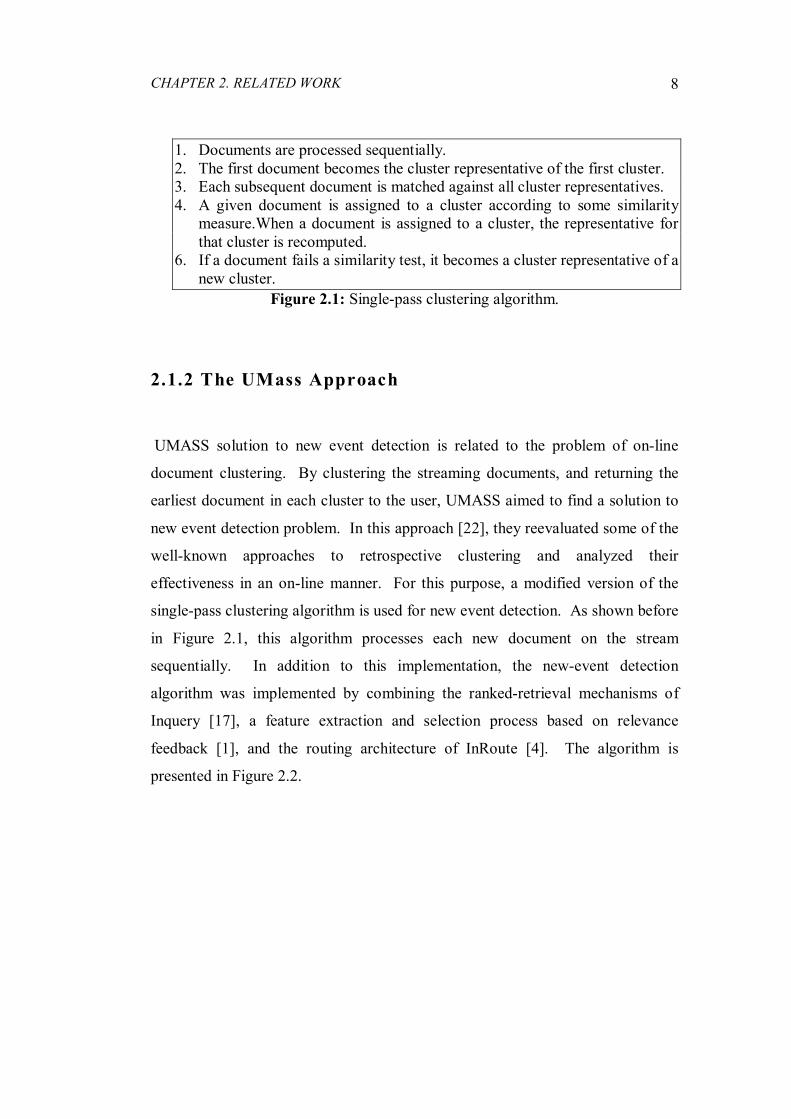
1. Documents are processed sequentially. 2. The first document becomes the cluster representative of the first cluster. 3. Each subsequent document is matched against all cluster representatives. 4. A given document is assigned to a cluster according to some similarity
measure.When a document is assigned to a cluster, the representative for that cluster is recomputed.
6. If a document fails a similarity test, it becomes a cluster representative of a new cluster.
Figure 2.1: Single-pass clustering algorithm.
2.1.2 The UMass Approach
UMASS solution to new event detection is related to the problem of on-line
document clustering. By clustering the streaming documents, and returning the
earliest document in each cluster to the user, UMASS aimed to find a solution to
new event detection problem. In this approach [22], they reevaluated some of the
well-known approaches to retrospective clustering and analyzed their
effectiveness in an on-line manner. For this purpose, a modified version of the
single-pass clustering algorithm is used for new event detection. As shown before
in Figure 2.1, this algorithm processes each new document on the stream
sequentially. In addition to this implementation, the new-event detection
algorithm was implemented by combining the ranked-retrieval mechanisms of
Inquery [17], a feature extraction and selection process based on relevance
feedback [1], and the routing architecture of InRoute [4]. The algorithm is
presented in Figure 2.2.

CHAPTER 2. RELATED WORK
9
1. Use feature extraction and selection techniques to build a query representation to define the document's content.
2. Determine the query's initial threshold by evaluating the new document with the query.
3. Compare the new document against previous queries in memory.
4. If the document does not trigger any previous query by exceeding its threshold, the document contains a new event.
5. If the document triggers an existing query, the document is not containing a new event.
6. (Optional) Add the document to the agglomeration list of queries it triggered.
7. (Optional) Rebuild existing queries using the document.
8. Add new query to memory. Figure 2.2: UMASS new event detection algorithm.
2.1.3 Dragon System Approach
The Dragon system used a language modeling approach of single word (unigram)
frequencies for cluster and document representations: their document
representation did not use tf× idf scores, as used in the UMASS system and the
CMU system. Dragon's cluster comparison methodology is based on the
KullbackLeibler distance measure [2]. They used a preprocessing step in which
an iterative k-means clustering algorithm was used to build 100 background
models (clusters) from an auxiliary corpus. Initially, the first story in the corpus is
defined as an initial cluster [2]. The remaining stories in the corpus are processed
sequentially; for each one, the “distance” to each of the existing clusters is
computed. In their decision process, a document is considered to contain a new
event when it is closer to a background model than to an existing story cluster.
As a modification, they introduced “decay term” to cause clusters to have
a limited existence in time. By adjusting the decay parameter and the overall
threshold the on-line detection system can be tuned.

CHAPTER 2. RELATED WORK
10
2.1.4 UPenn Approach
The UPenn approach used the single-link (nearest neighbor) clustering method to
characterize each event. This method begins with all stories in their own
singleton clusters. Two clusters are merged if the similarity between any story of
the first cluster and any story of the second cluster exceeds a threshold. As a
system parameter, a deferral period is defined to be the number of files (each
containing multiple stories) the system is allowed to process before it relates an
event with the stories contained in the files. To implement the clustering, the
UPenn approach takes the stories of each deferral period and creates an inverted
index. Then each story, in turn, is compared with all preceding stories (including
those from previous deferral periods). When the similarity metric for two stories
exceeds a threshold, their clusters are merged. The clusters of earlier deferral
periods cannot merge since they have already been reported. If a story cannot be
merged with an existing cluster, it becomes a new cluster, which means a new
event.
2.1.5 BBN Technologies' Approach
The BBN approach uses an incremental k-means algorithm in order to cluster the
stories. Although it is similar, the clustering algorithm they used is not precisely a
k-means algorithm, because the number of cluster, k is not given beforehand. For
every newcomer document, the algorithm tries to make appropriate changes and
modifications on the clusters, until no more change can be applied.
There are two types of metrics that are useful for the clustering algorithm:
“selection metric,” which is the maximum probability value of the BBN topic
spotting metric and “thresholding metric,” which is the binary decision metric to
add a story to a cluster. A score normalization method is used to produce
improved scores [35]. The algorithm, which is derived from Bayes' Rule, is
shown in Figure 2.3.

CHAPTER 2. RELATED WORK
11
1. Use the incremental clustering algorithm to process stories up to the end of the current modifiable window.
2. Compare each story in the modifiable window with the old clusters to determine whether each story should be merged with that cluster or used as a seed for a new cluster.
3. Modify all the clusters at once according to the new assignments. 4. Iterate steps (2)-(3) until the clustering does not change.
Figure 2.3: BBN new event detection algorithm.
2.1.6 On-Line New Event Detection in a Multi-Resource
Environment Kurt[20] used traditional vector space model to represent documents. In his MS
Thesis, the system assigns weights to terms by using tf× idf method. In order to
limit the similarity calculations between documents, time-penalty functionality
was added to the system [2, 36, 37]. In addition to novel threshold, which is very
similar with the one, used by Papka [22], another threshold, called “support
threshold,” is introduced in order to decrease the number of new event alarms. By
the help of this threshold, the number of false alarms can be decremented
enormously. The hypothesis was: If a new event is worth for alarming, it should
be supported by up-coming news in a short time. The algorithm is depicted in
Figure 2.4.
1. Prepare a vector space model of the document.
2. Remove the old documents that exceed the time window. 3. Calculate the similarities between the new document and existing
documents in the time window.
4. Calculate the decision score for the new document.
5. If the decision score is positive, then the document contains a new event. Calculate support value.
6. If the decision score is negative, the document does not contain a new event. Then, start event tracking process to find the similar stories.
7. If the support value of any event exceeds the support threshold, perform alarm process.
8. Add the new document to the time window.
Figure 2.4: New event detection and tracking algorithm.

CHAPTER 2. RELATED WORK
12
The system works on k-Nearest Neighbor (kNN) Algorithm and it detects
new events on-line, and at the same time, it performs event-tracking process.
A summary of on-line new event detection approaches is given in Table
2.1.
CMU UMass Dragon UPenn BBN Kurt
Term
weight
Ltc version
of tf-idf
tf-idf N/A tf-idf Probabil-istic tf-idf
Document
represent-
ation
Vector-
space
model
Query
representation
N/A Vector
space
model
Vector space
model
Vector space
model
Event
represent-
ation
Single-
pass
clustering
single-pass
clustering
k-means
clustering
Nearest
neighbor
clustering
Incremental
k-means
clustering
No clustering
Similarity Cosine
similarity
Previous
queries run on
new document
Distance
between
document
to clusters
Cosine
similarity
Probabilistic
similarity
Cosine
similarity
Time
window
Used Used Used N/A N/A Used
Table 2.1: The summary of on-line new event detection approaches (N/A means
no information is available).
2.2 Event Clustering Approaches
Event clustering is an unsupervised problem where the goal is to automatically
group documents by events that may exist in the data. The significant difference
from supervised methods is that the supervised clustering needs training
documents about each event to formulate a classifier, while the unsupervised
setting operates without training documents. On the other hand, new event
detection problem is also unsupervised because no training documents are
required for processing the data, however, different from event clustering, the goal

CHAPTER 2. RELATED WORK
13
of new event detection is to separate documents that discuss new events from
documents discussing existing events.
Most of the news classification research prior to Topic Detection and
Tracking (TDT) deals with classification problems using topics instead of events.
For example, Hayes et al. [16] describe a news organization system in which a
rule-based approach was used to group 500 news stories into six topics. The
filtering problem analyzed at the Text Retrieval Conferences [18], is another
example of topic-based news classification. However, some event-based research
has been reported prior to the first TDT workshop [24].
A data structure for news classification, called “Frames,” is introduced in
1975 by R. Schank. [29]. The frames are constructed manually and are coded for
a semantic organization of text extracted by a natural language parser. Frames
contain slots for structured text that can be organized at different semantic levels.
For example, frames can be coded to understand entire stories [15], or for
understanding the parts of a person's name [11].
A frame-based system that attempted to detect events on a newswire was
constructed by DeJong in 1979 [14]. He used pre-specified software objects
called sketchy scripts. Frames and scripts for general news events such as
“Vehicular Accidents”' and “Disasters” were constructed by hand. The goal of his
system was to predict which frame needed to be populated. This system was
working mainly as a natural language parser, but as a side effect, it decided
whether a document contains an event. However, it did not detect new events.
In 1997, Carrick and Watters introduced an application that matched news
stories to photo captions using a frame-based approach modeling proper nouns
[11]. They claimed that, when the extracted lexical features are used, their frame-
based approach was nearly as effective as using the same features in a word
matching approach. Another research related to frame-based representations on
news data are discussed at Message Understanding Conferences (MUC) [23].
In order to represent different aspects of the natural language parse, frames
can be used helpfully; however, as new types of events appear and existing events

CHAPTER 2. RELATED WORK
14
grow in a news environment, it is difficult to maintain the number of frames and
the details of their contents.
In general, the previous approaches to clustering were used in a
retrospective environment where all the documents were available to the process
before clustering begins. In his dissertation [22], Papka tested previous
approaches to document clustering and he evaluated their effectiveness for online
event clustering. He applied retrospective approaches to an online environment.
He reevaluated single-link, average-link, and complete-link hierarchical
agglomerative clustering strategies, but use them in a single-pass (incremental)
clustering context, in which a cluster is determined for the current document
before looking at the next document.
2.3 Document Clustering Approaches
Document clustering is an unsupervised process that groups documents similar to
each other. Since the clustering algorithm does not need any training instance or
any information describing the group, the problem of clustering is often known as
automatic document classification. Clustering has been studied extensively in the
literature [19], and the common element among clustering methods is a model of
word co-occurrence that is applicable to text classification problems in general.
By using this model, constructed clusters contain documents consist of words
common to most of the documents into that cluster. A historical account of
clustering research is given by van Rijsbergen [33], who also discusses cluster
similarity coefficients applied to simple word matching techniques. In another
research, Salton [25] discusses clustering approaches that use tf× idf
representations for text. In addition, Croft [12] introduced a probabilistically
based clustering algorithm, and several works have been presented, including by
TDT participants in the context of event clustering [2, 35].
Document clustering is also used for information retrieval purposes. The
goal of information retrieval system is to retrieve documents, which are relevant
to the query of a user. One of well-known query processing approach is cluster-

CHAPTER 2. RELATED WORK
15
based retrieval (CBR), which is a method for improving document retrieval in
terms of speed and effectiveness [27, 25]. There are many researches about CBR
[25, 28, 15, 33]. These approaches are based on the “cluster hypothesis,” which
states, “closely associated documents tend to be relevant to the same request,”
[33]. However, some databases do not obey this hypothesis, whereas some do
[34]. The results presented by Voorhees [34] as well as Croft [13] imply that some
collections and requests benefit from pre-clustering, while others do not.
Furthermore, according to Can [6], no CBR approach is better than full search
(FS), one of the well-known query processing approach, in terms of space and
time.
The previous work, which most influenced our approach to new event
detection and clustering, is based on single-pass clustering [33] and Cover
Coefficient based Clustering Methodology (C3M) [8]. In the remainder of this
section, a brief description of these methods is provided.
2.3.2 Single-Pass Clustering
Single-pass clustering or incremental clustering is an approach for creating
clusters on-line. The algorithm is discussed by van Rijsbergen [33] and depicted
before in Figure 2.1.
The single-pass algorithm sequentially processes documents using a pre-
specified order. The current document is compared to all existing clusters, and it
is merged with the most similar cluster if the similarity exceeds a certain
threshold, otherwise it starts its own cluster. The single-pass algorithm results in
faster processing than the agglomerative hierarchical clustering algorithm, even
though both approaches have an O(n2) asymptotic running time. The main
disadvantage of the single-pass method is that the effectiveness of the algorithm is
dependent on the order in which documents are processed. This is not a problem
in event clustering, because the order is fixed.

CHAPTER 2. RELATED WORK
16
2.3.3 Cover Coefficient-based Clustering Methodology
The C3M algorithm is a partitioning-type clustering algorithm, which means that
clusters cannot have common documents, and the algorithm operates in a single-
pass approach. The algorithm consists of three main parts:
• Select the cluster seeds; C3M is one of the nonhierarchical clustering
algorithms, and it is seed-based. The chosen seed must attract relevant
documents onto itself. To perform this issue, it must be calculated in a
multidimensional space that, how much seed document covers non-seeds
and what the amount of similarity is.
• Construct clusters; group the non-seed documents around the selected
seeds.
• Group documents into a ragbag cluster, which are not fit to any cluster.
C3M is covered in more details in the next chapter.

17
Chapter 3
Cover Coefficient-based
Clustering Methodology: C3M As mentioned in the second chapter, one of the previous work that most
influences our approach to new event detection and clustering is based on Cover
Coefficient based Clustering Methodology (C3M) [8]. In the remainder of this
chapter, we explain this clustering method in more details.
The C3M algorithm is a single-pass partitioning-type clustering algorithm,
which means that clusters cannot have common documents. The algorithm has
three parts, the first part determines the number of clusters and the cluster seeds,
the second part groups the non-seed documents around the selected seeds, and the
last part gathers the documents that are not fit to other clusters, into a ragbag
cluster. A brief description of the algorithm is shown in Figure 3.1.
The complexity of the algorithm is O(m × xd × tgs). In this expression, xd
is the average number of distinct terms per document, tgs is the average number of
seed documents per term, and m is the number of documents in the database [8].

CHAPTER3. COVER COEFFICIENT-BASED CLUSTERING METHODOLOGY
18
Figure 3.1: C3M Algorithm.
C3M is seed-based. The chosen seed must attract relevant documents onto
itself. To perform this complete operation, seed value must be calculated in a
multidimensional space with respect to the coverage of non-seed documents and
the amount of similarity. Using the cover coefficient (CC) concept, these
relationships are reflected in the C matrix. The algorithm constructs a C matrix
by using a D matrix that contains whole data before clustering begins, and it is a
document by term (m × n) matrix. A sample D matrix is shown below:
Figure3.2: Sample D Matrix.
654321 tttttt
5
4
3
2
1
000101110000110001001111101001
ddddd
C3M:
1. Determine number of clusters and cluster seeds.
2. Construct the clusters:
i = 1;
repeat;
if di is not a cluster seed
then
begin;
Find the cluster seed (if any) that maximally covers di; if there is
more than one cluster seed that meets this condition, assign
di to cluster whose seed power value is the greatest among
the candidates;
end;
i = i+1;
until i>m.
3. If there remain unclustered documents, group them into a ragbag cluster (some
nonseed documents may not have any covering seed document).
CHAPTER3. COVER COEFFICIENT-BASED CLUSTERING METHODOLOGY
19
By definition of Can and Özkarahan [8]: “A D matrix that represents the
document database {d1, d2, ….dm} described by the index terms T={t1, t2, ….tn} is
given. The CC matrix, C, is a document-by-document matrix whose entries cij
(1 ≤ mji ≤, ) indicate the probability of selecting any term of di from dj.”
In the Figure 3.2, each row indicates one document, and each column
indicates one individual term. To able to represent a document in D matrix, each
document must have at least one term and each term must appear at least in one
document. D matrix can be generated manually or automatically. On the other
hand C matrix is a document-by-document matrix whose entries, cij values,
indicate the probability of selecting any term of document (di) from document (dj),
where di and dj are the members of D matrix.
Two-phase experiment must be processed to generate C matrix. The C
matrix summarizes the results of two-phase experiment. At first phase the
algorithm chooses a term randomly from the terms of di, from the selected term
then it tries to draw dj. The sum of the probability values to select dj from di
forms cij, which is the member of C matrix. The best way to explain this issue is
using an analogy. It would be helpful to repeat the same analogy that is used by
Can and Özkarahan [8] about two-phase experiment: “Suppose we have many
urns and each urn contains balls of different colors. Then what is the probability
of selecting a ball of a particular color? To find this probability experimentally,
notice that first we have to choose an urn at random, and then we have to choose a
ball at random. In terms of the D matrix, what we have is the following: From
the terms (urns) of di, choose one at random. Each term appears in many
documents, or each urn contains many balls. From the selected term, try to draw a
ball of a particular color. What is the probability of getting dj, or what is the
probability of selecting a ball of a particular color? This is precisely the
probability of selecting any term of di from dj, since we are trying to draw the
selected term of di from dj at the second stage.”
If we consider iks is the event of first stage, and iks′ is the event of second
stage, then the probability P( iks , iks′ ) can be represented as P( iks )× P( iks′ ) [17].

CHAPTER3. COVER COEFFICIENT-BASED CLUSTERING METHODOLOGY
20
By using iks and D matrix, we can construct S probability matrix. Multiplying S
matrix with the transpose of S ′ ( TS ′ ) forms the m-by-m C matrix. For example,
by using D matrix in Figure 3.2, constructed S and TS ′ matrixes are shown in
Figure 3.3.
S =
0002/102/12/12/100003/13/10003/1
004/14/14/14/13/103/1003/1
, TS ′ =
0002/104/13/12/100003/12/10004/1
002/12/114/13/102/1004/1
Figure 3.3: S and TS ′ matrixes derived from the D matrix of Figure 3.2.
By multiplying the two matrixes in Figure 3.3, the C matrix, in Figure 3.4,
is constructed.
375.00.0125.0375.0125.00.0417.0417.00.0167.0
083.0277.0361.0083.0194.0188.00.0063.0563.0188.0083.0111.0194.0250.0361.0
Figure 3.4: Sample C matrix.

CHAPTER3. COVER COEFFICIENT-BASED CLUSTERING METHODOLOGY
21
Calculation of one element of the C matrix is shown below:
250.003100
21
31
21010
41
31
*
12
6
12112
=×+×+×+×+×+×=
′=∑=
c
ssck
kk
The entries of the C matrix can be defined as follows:
∑=
′×=n
kkj
Tikij ssc
1 where jkkj
T ss ′=′
This equation can be rewritten as:
,1∑
=
×××=n
kjkkikiij ddc βα 1≤ mji ≤, (3.1)
Where; iα and kβ are the reciprocals of the thi row sum and the thk
column sum, respectively, as shown below:
1
1
−
=
= ∑
n
jiji dα , 1 ≤ ,mi ≤ (3.2)
1
1
−
=
= ∑
m
jjkk dβ , 1 ≤ ,nk ≤ (3.3)
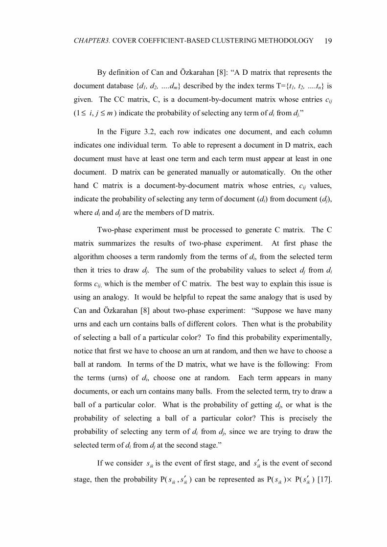
Some properties [7] of the C matrix are depicted in Figure 3.5. The proofs
of properties 1-4 are given in [7] and [10]. The proof of property 5 is given in [9].
CHAPTER3. COVER COEFFICIENT-BASED CLUSTERING METHODOLOGY
22
1. For 0,0, >≤≤≠ iiiiij cccji ( iiij cc > is possible for weighted D matrix).
2. 1...21 =+++ imii ccc (Sum of row i is equal to 1 for 1≤ mi ≤ ).
3. If non of the terms of di is used by the other documents, then iic =1; otherwise, iic <1.
4. If ijc = 0, then jic = 0, and similarly, if ijc > 0, then jic > 0; but in general,
jiij cc ≠ .
5. iic = iic = ijc = jic iff di and dj are identical.
Figure 3.5: Some properties of the C matrix.
The diagonal values of the C matrix ( iic ) is called decoupling coefficient,
and is denoted with the symbol iδ . This measure shows how much the
documents is not related to the other documents. On the contrary, coupling
coefficient is calculated by using ith row off-diagonal entries sum, it is denoted
with the symbol iψ . This coefficient indicates the extent of coupling of di with
the other documents of the database. The concepts of decoupling and coupling
coefficients, iδ ′ and iψ ′ , are the counterparts of the same concepts defined for
documents.
iδ = iic : Decoupling coefficient of di.
iψ = 1 - iδ : Coupling coefficient of di.
By following a methodology similar to the construction of the C matrix, a
term-by-term (n × n)C ′ matrix of size n by n can be formed for index terms. C ′
has the same properties with C matrix. As with the C matrix, the C ′ matrix
summarizes the results of a two-stage experiment in a term-wise manner. C ′
matrix can be defined as follows:
∑=
×××=′m
kkjkkiiij ddc
1αβ
1≤ nji ≤, (3.4)

CHAPTER3. COVER COEFFICIENT-BASED CLUSTERING METHODOLOGY
23
As mentioned before, the C3M Algorithm is seed based. In order to select
seed documents, cluster seed power for all documents is calculated, by using the
following formula:
∑=
××=n
jijiii dP
1ψδ (3.5)
This equation is used for binary D matrix, which means that; if the term
occurs in the document, the term frequency is taken as 1, it is taken as 0
otherwise. iδ provides the separation of clusters, iψ provides the connection
among the documents within a cluster, and summation provides normalization.
For weighted matrix, a modified version of cluster seed power formula is used:
∑=
′×′×××=n
jjjijiii dP
1)( ψδψδ (3.6)
After cluster seed power applied to the documents, the document that has
highest seed power is selected as candidate. Because this procedure can produce
identical seeds, to eliminate these false seeds, a threshold value is used. All
documents are sorted by their seed power values, so that identical documents are
grouped into the sorted list. If the value, which is obtained by comparing their C
matrix values is smaller than threshold value then it means that we have a false
seed. For each false seed, another document from the sorted list is considered.
This process can be applied on-line with some modifications. In the on-
line clustering environment, each document is analyzed sequentially and is either
placed into an existing cluster or initiates a new cluster and thus becomes a cluster
seed. In our approach we do not have falsified seeds, thus we do not apply false
seed elimination process. How the concepts of C3M algorithm applied to on-line
clustering and on-line event detection is the subject of Chapters 5 and 6,
respectively.

24
Chapter 4
Experimental Data and Evaluation Methods
4.1 TDT Corpus
In our experiments, we used TDT1 corpus, which is also used by the participants
of TDT pilot study. In order to support the TDT study effort, Linguistic Data
Consortium (LDC) has developed this corpus using text and transcribed speech.
TDT1 covers the documents containing news from July 1, 1994 to June 30, 1995
and includes 15,863 stories. About half of the data is taken from Reuter’s
newswire and half from CNN broadcast news transcripts. The transcripts were
produced by the Journal of Graphics Institute (JGI). The stories in this corpus are
arranged in chronological order, are structured in SGML format that has a size of
53,563 KB, and are available on the LDC web page (http://www.ldc.upenn.edu/).
A set of 25 target events has been chosen from TDT1 to support the TDT
study effort. These events include both expected and unexpected events. They
are described in some detail in documents provided as part of the TDT Corpus.
The TDT corpus was completely interpreted with respect to these events, so that
each story in the corpus is appropriately flagged for each of the target events

CHAPTER4. EXPERIMENTAL DATA AND EVALUATION METHODS
25
discussed in it. There are three possible flag values: YES (the story discusses the
event), NO (the story does not discuss the event), and BRIEF (the story mentions
the event only briefly, or merely references the event without discussion; less than
10% of the story is about the event in question). Flag values for all events are
available in the file “tdt-corpus judgments” with stories.
The average document contains 460 (210 unique) single-word features
after stemming and removing stop-words. The names of all 25 events chosen
from the TDT1 Corpus are listed in Figure 4.1.
Figure 4.1: Judged 25 events in TDT corpus.
1. Aldrich Ames spy case 2. The arrest of 'Carlos the Jackal' 3. Carter in Bosnia
4. Cessna crash on White House lawn 5. Salvi clinic murders
6. Comet collision with Jupiter 7. Cuban refugees riot in Panama
8. Death of Kim Jong II 9. DNA evidence in OJ trial
10. Haiti ousts human rights observers 11. Hall's helicopter down in N. Korea
12. Flooding in Humble, Texas 13. Breyer's Supreme Court nomination
14. Nancy Kerrigan assault 15. Kobe Japan earthquake
16. Detained U.S. citizens in Iraq 17. New York City subway bombing
18. Oklahoma City bombing
CHAPTER4. EXPERIMENTAL DATA AND EVALUATION METHODS
26
The judgments were obtained by two independent groups of assessors and
then reconciled to form a set of final judgments. Documents were judged on a
ternary scale to be irrelevant, to have content relevant to the event, or to contain
only a brief mention of the event in a generally irrelevant document. We use 1124
relevant documents in the experiments after eliminating briefs and overlaps.
4.2 Evaluation
4.2.1 Effectiveness Measures
It is desirable to have one measure of effectiveness for cross system comparisons.
Unfortunately, no measure uniquely determines the overall effectiveness
characteristics of a classification system. Several definitions for single valued
measures have emerged, and are reviewed by van Rijsbergen [33]. One
widespread approach is to evaluate text classification using F1 Measure [21],
which is a combination of recall and precision and it is defined later.
Since there does not exist an agreed upon single valued metric that
uniquely captures the accuracy of a system, it is often the case that two or more
measures are needed, and efforts to define combination measures do not
necessarily lead to an applicable measure of usefulness. In what follows, we
assume usefulness is a function of user satisfaction with the classification
effectiveness of a system. In practice, usefulness is constantly changing; one
system can be useful for some particular purpose, while it would be useless for
others. For example, consider two systems: a car alarm and a radar system for an
aircraft guiding a missile. Car alarm system may sound occasionally, especially
when it is set to oversensitive. It may be acceptable to sound occasionally when
no theft event exists, but if an alarm does not sound during an actual theft, this
means that the system is useless. In other words, the owner of the car has a low
tolerance for false alarms and no tolerance for misses. On the other hand, radar

CHAPTER4. EXPERIMENTAL DATA AND EVALUATION METHODS
27
system has a different usefulness function. It may be tolerable for the system to
miss a target, but a false targeting may cause a disaster. With these requirements
in mind, without inventing another measure, we report several effectiveness
measures, which have been previously used for the analysis of text classification
experiments.
Text classification effectiveness is often based on two measures. It is
common for information retrieval experiments to be evaluated in terms of recall
and precision, where recall measures how well the system retrieves relevant
documents and classify them correctly, and precision measures how well the
system distinguishes relevant documents from irrelevant ones in the set of
retrieved group. In addition, F1 measure [21] is used, which is the combination of
recall and precision. In TDT, and the work described here, system error rates are
used to evaluate text classification. These errors are system misses and false
alarms. The accuracy of a system improves when both types of errors approaches
to zero. In new event detection, misses occur when the system does not detect a
new event, and false alarms occur when the system indicates a document contains
a new event when in truth it does not. In addition to system error rates, we report
performance (pfr), which is based on the Euclidean distance average miss rate and
false alarm rate from the origin.
The methods for calculating the effectiveness measures for on-line event
clustering, and on-line new event detection are summarized below using modified
version of Swets’s [31] two-by-two contingency table (Tables 4.1 and 4.2):
Relevant Non-Relevant
Retrieved a b
Not Retrieved c d
Table 4.1: Two-by-two contingency table for event clustering.

CHAPTER4. EXPERIMENTAL DATA AND EVALUATION METHODS
28
Where the retrieved documents in the table are those that have been
classified by the system as positive instances of an event, and the relevant
documents are those that have been manually judged relevant to an event.
New is True Old is True
System Predicted New a b
System Predicted Old c d
Table 4.2: Two-by-two contingency table for event detection.
Assuming S represents the set of retrieved documents, and S ′ represents
the set of not retrieved documents, then:
a = number of documents in S discussing new events,
b = number of documents in S not discussing new events,
c = number of documents in S ′ discussing new events,
d = number of documents in S ′ not discussing new events;
By using the two-by-two contingency table, we can derive the
effectiveness measures as follows:
Recall = ca
aR+
= , (4.1)
Precision = ba
aP+
= , (4.2)
F1 Measure = RP
PR+
2 , (4.3)
Miss Rate = ac
cM+
= , (4.4)
False Alarm Rate = db
bFA+
= , (4.5)
Distance from Origin = 22 FM + , (4.6)
Performance (pfr) = 100 - Distance from Origin. (4.7)

CHAPTER4. EXPERIMENTAL DATA AND EVALUATION METHODS
29
The difference between event clustering and new event detection about
effectiveness calculations is that; for the former, two-by-two contingency table is
formed for each cluster that is selected as the best cluster for that event, and the
overall system effectiveness is calculated by taking the averages of each measure.
For the later, there is only one contingency table formed, and the effectiveness
measures are computed by using Table 4.2.
In the experiment results, effectiveness measures are given as rates, except
the performance (pfr).
4.2.1 Experimental Methodology
The experiments of both event detection and event clustering are executed on a
personal computer, which has Intel Pentium 550 Mhz. Central Processor Unit
(CPU) and has 128 MB of main memory.
It is considered that a time gap between bursts of topically similar stories
is often an indication of different events. It is also experienced that events are
typically reported in a brief time window (e.g., 1-4 weeks) [22]. These
determinations in mind, we applied a time windowing in days to limit the size of
comparisons. We see that time windowing influenced the CPU time. In other
words, evaluating more days results with more CPU time.
4.2.2 Preprocessing
In the preprocessing phase, we eliminate stop words from the corpus by the help
of a pre-constructed stop word list. This list consists of terms like (a, an, and, the)
that are fatal importance to the structure of English grammar (stop word list is
attached to the appendix part). In order to able to find the terms, which have the
same root, we apply Porter’s stemming algorithm [30] to the corpus. We get
stemmed word list consists of 72,034 terms and phrases. At the same time, we

CHAPTER4. EXPERIMENTAL DATA AND EVALUATION METHODS
30
construct the document vectors in the format of <docno, termno, termfrequency>
as shown in Figure 4.2. We get 15,863 document vectors containing this format.
DOC1: 1:1:2:1:3:1:4:1:5:1:6:1:7:1:8:1
DOC2: 9:1:10:1:11:1:12:1:13:1
DOC3: 3:1:6:1:15:1:16:1:17:1
DOC4: 6:1:16:1:17:1
DOC5: 2:1:3:1:4:1:5:1:7:1:8:1:17:1
.
.
DOCn: . . . . . . . . . . .
Figure 4.2: An example document vector.
This structure is used during both on-line event clustering and on-line
event detection experiments.

31
Chapter 5
On-Line Event Clustering
In this chapter, we focus on the problem of on-line mode of event clustering. We
introduce a new algorithm as a solution to the problem, with the help of C3M
algorithm.
5.1 Window Size
In our experiments, we add window size concept to the algorithm. This
prevents producing oversized clusters, and gives equal chance to all documents to
be a cluster seed. When we analyze the distribution of documents for a particular
event, we determine that the most of the documents for an event ends in a few
days from the first occurrence of that event. There are exceptions for some
events, which lasts for the most days of the year. For example, events 9, 22, 25,
listed in Table 5.1, do not follow this tendency. The details are shown in Table
5.1.
In Table 5.1, number of documents are counted for the first 10, 20, 30, 40
days of each event, and for the whole life of that particular event, that is; from the
first occurrence to the last story about that event. The table summarizes that,
stories about most of the events appear in first 30 or 40 days. At the end of the

CHAPTER 5. ON-LINE EVENT CLUSTERING
32
table, total number of documents shows a trend that the most significant window
sizes are these two day-periods.
No. of Documents in Window Events
Event Life in Days Life 40 30 20 10
1. Aldrich Ames spy case 96 8 6 5 3 2
2. The arrest of “Carlos the Jackal” 30 10 10 10 9 7
3. Carter in Bosnia 49 30 29 29 27 25
4. Cessna crash on White House lawn 2 14 2 2 2 2
5. Salvi clinic murders 60 41 34 34 33 33
6. Comet collision with Jupiter 121 45 44 44 44 6
7. Cuban refugees riot in Panama 3 2 2 2 2 2
8. Death of Kim Jong II 317 56 45 44 41 36
9. DNA evidence in OJ trial 376 114 29 12 7 4
10. Haiti ousts human rights observers 3 12 12 12 12 12
11. Hall's helicopter down in N. Korea 20 97 97 97 97 50
12. Flooding in Humble, Texas 8 22 22 22 22 22
13. Breyer's Supreme Court nomination 80 7 6 6 6 5
14. Nancy Kerrigan assault 180 2 1 1 1 1
15. Kobe Japan earthquake 127 84 82 81 81 74
16. Detained U.S. citizens in Iraq 54 44 33 32 29 11
17. New York City subway bombing 8 24 24 24 24 24
18. Oklahoma City bombing 45 273 261 249 226 215
19. Pentium chip flaw 9 4 4 4 4 4
20. Quayle's lung clot 9 12 12 12 12 12
21. Serbians down F16 10 65 65 65 65 65
22. Serb's violation of Bihac safe area 130 90 1 1 1 1
23. Faulkner's admission into the Citadel 180 7 4 4 3 3
24. Crash of US Air flight 427 140 39 37 37 36 35
25. World Trade Center bombing 360 22 1 1 1 1
Total number of documents: - 1124 863 832 790 654
Table 5.1: Distribution of the documents in time (window size in days).

CHAPTER 5. ON-LINE EVENT CLUSTERING
33
This distribution of documents is depicted in more details for a specific
event (event number 18). It has the maximum number of related stories (273)
among 25 events. Figure 5.1, is borrowed from Papka [22], illustrates the window
size concept. In this figure, we see that the most of the news about “Oklahoma
city bombing” appeared between the days of 293 and 305 (in the fist ten days).
After the second week of first occurrence of the event, it is observed that the
amount of streaming news is reduced. Most of the events in TDT1 corpus behave
as the event seen in this figure.
Figure 5.1: Event evolution; Oklahoma city bombing (adapted from Papka[22])
This tendency in mind, we use a window size concept, in order to improve
the performance of the system. The hypothesis is that; limiting the number of
documents, by processing only the documents in predetermined window size
would help to improve the effectiveness of the system. This hypothesis is verified
for events following the same tendency. However, as a disadvantage, the miss
rate of the system is increased dramatically for the events, which do not follow the
common trend.
In order to improve the performance, Papka [22] used time windowing in
his system. The main motivation of his approach is that documents closer
together on the stream are more likely to discuss similar events than documents
further apart on the stream. As depicted in Figure 5.1, when a significant new

CHAPTER 5. ON-LINE EVENT CLUSTERING
34
event occurs there are usually several related documents in the initial days. Over
time, coverage of old events is displaced by events that are more recent. Different
from our approach, Papka integrated time in the thresholding model.
5.2 Threshold Model
In the seed selection process, we apply a threshold model, which varies from
document to document. For on-line clustering subject, we aimed to find a way of
putting a threshold in front of the documents, to make the decision of flagging as
seed. Without thresholding all the documents in the corpus would be a seed, and
this would produce number of clusters equals to the number of documents in the
corpus. This is not a desired situation for event clustering. On the other hand,
when a greater value is used as a threshold, the system would give unproductive
results; in other words, the miss rate of the system would be unacceptable. Thus,
we want an appropriate number of clusters for each individual event. It is
acceptable for the system to produce at least one representative cluster for each
event; while doing this the system must classify the related stories into that
clusters. In other words, we don’t desire weak or empty clusters (without member
except the seed). As a solution, we use a threshold concept, by computing the
average P value for documents in the scope of predetermined window size, and
compare this value to the iP value of new coming document. The expression of
threshold Tr is given below:
Tr = ∑∈windowd
ii
P / (No. of documents in window) (5.1)
The idea behind this approach is that; iP value is a sign for a document
how the document is different from the others, if this value can exceed the average
P value, this means that the particular document reviews a different story, and it
deserves to be a seed of a new cluster.

CHAPTER 5. ON-LINE EVENT CLUSTERING
35
5.3 The Algorithm The on-line event-clustering algorithm constructs the cluster structure by
processing document vectors sequentially in a sing-pass manner; a simple
example of the document vector structure is given in Figure 4.2. The algorithm is
shown in Figure 5.2.
When a document (say di) arrives, the update process begins if the
difference between the dates of the oldest document and the youngest one exceeds
the pre-determined window size. In the update process, system deletes the old
documents until the date difference falls under the value of window size. If the
deleted document is a seed of a cluster, the whole cluster is deleted after
computing its effectiveness. However, the members of the deleted cluster, which
do not exceed the window size, remain in the system and they are used in the
For each new coming document di;
1. let dj= oldest document
2. if diDate– djDate* ≥ predetermined window size (WS)
repeat;
delete dj
if dj is seed
delete cluster started by dj
dj= oldest document in WS
until diDate– djDate < WS
3. calculate the seed power value iP
4. determine the threshold (Tr)
5. if iP ≥ Tr
label the document as seed and initiate a new cluster
else
if there exists any cluster
calculate cij value to decide which cluster it is attached
else
put the document in a ragbag cluster
(*) djDate = 0 if there is no previous document in the window.
Figure 5.2: On-line event clustering algorithm.
CHAPTER 5. ON-LINE EVENT CLUSTERING
36
computation of β values. For the next step, the seed power ( iP ) of the document
di, and then the threshold for the same document are calculated. If seed power
value of the document, exceeds the threshold, then it is labeled as a new seed, and
a new cluster is initiated. Otherwise, the similarity calculations are done. That is;
the similarities between the document and the previous seed documents are
computed, and the document is classified as a member of the cluster of the seed
document, which constitutes the maximum similarity with the current document
di. If there is no cluster formed, or all clusters are deleted during the update
process, the document is put in a ragbag cluster.
In Figure 5.2, diDate and djDate demonstrate the date of new coming
document and the date of the oldest document in the window size respectively.
Ragbag cluster is a cluster that gathers the non-seed documents, which have no
common terms with current seeds, or there is no cluster introduced in the window
size.
Different from C3M algorithm, in on-line event clustering algorithm, once
a document is determined as a seed, it stays as seed until it leaves the system.
Recall that in C3M algorithm, when a document joins to a cluster it may influence
the centroid of that cluster. This is not the point in our clustering strategy.
Because the idea is that when a document is selected as a seed document, then the
only information to pull the other documents is the seed document itself. When a
document is selected as a seed, it always remains the same and it is used as the
cluster centroid.
5.3.1 An Operational Example
Generation of Clusters
To make the algorithm more understandable, we give an example using
the sample D matrix of Chapter 3. Assume that the system receives the

CHAPTER 5. ON-LINE EVENT CLUSTERING
37
documents one at a time, and d1, d2 and d5 discuss the same event while d3 and d4
discusses a different event (actually we have two events).
When d1 arrives:
1δ =1 => 1ψ = 0 => 1P = 1 × 0 × 3 = 0
Tr = 010 =
1P = Tr => d1 is flagged as seed and it forms Cluster-1.
When d2 arrives:
2δ = 0.75 => 2ψ = 0.25 => 2P = 0.75 × 0.25 × 4 = 0.75
Tr = 38.02
75.00 =+
2P > Tr => d2 is flagged as seed and it forms Cluster-2.
When d3 arrives:
3δ = 0.61 => 3ψ = 0.39 => 3P = 0.61 × 0.39 × 3 = 0.71
Tr = 49.03
71.075.00 =++
3P > Tr => d3 is flagged as seed and it forms Cluster-3.
When d4 arrives:
4δ = 0.41 => 4ψ = 0.59 => 4P = 0.41 × 0.59 × 2 = 0.48
Tr = 49.04
48.071.075.00 =+++
4P < Tr => cij values must be calculated for d4 as illustrated before
in Chapter 3, and classified with the seed document that has the highest similarity
with cij.
By using Equations 3.1, 3.2, and 3.3:

CHAPTER 5. ON-LINE EVENT CLUSTERING
38
21
4 =α and 31,
21
65 == ββ => then;
( )
42.01251
3111
2110000
21
000000021
17.0611
31100000
21
43
42
41
==
××+××++++×=
=+++++×=
==
××+++++×=
c
c
c
d4 goes to Cluster-3,
since the similarity value between d4 and d3 is more than the others.
When d5 arrives:
5δ = 0.38 => 5ψ = 0.62 => 5P = 0.38 × 0.62 × 2 = 0.47
Tr = 48.05
49.048.071.075.00 =++++
5P < Tr => cij values must be calculated for d5.
By following the same procedure:
12.038.012.0
53
52
51
===
ccc
d5 goes to Cluster-2.
The clusters are shown in Figure 5.3.
Cluster-1 Cluster-2 Cluster-3 + : Cluster seed.
* : Member document relevant to the event started by the cluster seed.
# : Member document not related to the event started by the cluster seed.
Figure 5.3: Final event clusters.
In Figure 5.3, the seed documents, the relevant members, and non-relevant
members are represented by the symbols (+, *, and #) respectively. In order to
d1
+
d2
# dn +
d5 *
d3
+
d4 *

CHAPTER 5. ON-LINE EVENT CLUSTERING
39
show false alarm measure, an extra document dn is added to Cluster-2
intentionally.
Calculation of Effectiveness Measures
In the effectiveness process, for each event, we choose the best cluster from the
clusters related to the same event, note that the cluster seed determines the related
event of the corresponding cluster. The best cluster is the one that contains the
maximum number of the stories of the related event. For example, consider that
clusters 1 and 2 contain the documents discussing the same event; Cluster-2 is
chosen as the best cluster, because it contains more number of relevant elements.
Cluster 3 is the only cluster related to the next event; therefore, we include it in
our computations. Performance is computed with the help of measures covered in
Chapter 4. The results are given in Figure 5.4. Window size notion is not applied
to this sample data, because it is very small when compared to the data used in our
experiments.
Relevant Non-Relevant
Retrieved 2 1
Not Retrieved 1 2
Two-by-two contingency table for Cluster-2
Relevant Non-Relevant
Retrieved 2 0
Not Retrieved 0 4
Two-by-two contingency table for Cluster-3 With the help of effectiveness measures that covered in Chapter 4:
Recall Precision F1 Miss False Alarm
Cluster-2 0.67 0.67 0.67 0.33 0.33
Cluster-3 1 1 1 0 0
Pooled Avg. 0.84 0.84 0.84 0.17 0.17
System performance.
Figure 5.4: Effectiveness measure results for the example data.

CHAPTER 5. ON-LINE EVENT CLUSTERING
40
5.4 Experimental Results
We obtain two sets of experimental results, one set for binary D matrix and one
set for weighted. For the first set, the system takes the term frequencies of
document vectors as binary, in other words if a particular term exists in the vector
the system takes its term frequency as 1, it is taken as 0 otherwise. In order to
calculate the iP value, equation (3.5) is used. For the second set, the system
incorporates the actual term frequencies into equation (3.6). For example, if a
term appears in a document 10 times, term frequency (dij) is taken as 10.
5.4.1 Results of Binary Implementation
For obtaining binary implementation results, we execute the algorithm six times
for six different window sizes. The idea behind this execution method is that; we
aim to see the impact of different window sizes to the effectiveness results. For
each window size, the best clusters are chosen, and pooled average of
effectiveness results, containing all 25 events, is computed. These results are
depicted in Table 5.2.
EVENT CLUSTERING (BINARY)
W-SizeRecall
% Precision
% F1 %
Miss %
F-Alarm
% Performance(pfr)15 25 75 35 75 0.8 25 20 27 77 37 73 0.8 27 25 28 75 38 72 0.6 28 30 30 73 39 70 0.7 30 35 31 73 39 69 0.8 31 40 29 70 37 71 0.7 29
Table 5.2: Event clustering results according to six window sizes (binary).
In Table 5.2, we observe that; while window size expands, the probability
of retrieving relevant documents improves, in other words recall improves, until a

CHAPTER 5. ON-LINE EVENT CLUSTERING
41
peak point of this improvement, which is the window size of 35. The
experiments, after this point for windows 40, 45 and 50, show that the
performance (prf) suffers. On the contrary, general trend of precision is negative,
since the number of retrieved documents increases with the increase of window
size. The performance(pfr) measure has the same trend with recall, and it shows
that the best performance(pfr) is obtained with the window size 35. Change of
effectiveness measures and change of performances (pfr) in terms of different
window sizes are illustrated in Figures 5.5 and 5.6.
0%10%20%30%40%50%60%70%80%90%
15 20 25 30 35 40
Window Size
RecallPrecisionF1Miss
Figure 5.5: Change of effectiveness measures vs. window size (binary).
In the experiments of binary implementation, one of the events, “Cuban
refugees riot in Panama,” which has the event number of 7, cannot be clustered,
because the documents of this event cannot be chosen as seed. For this reason,
while computing the pooled averages, the effect of this event to the results reflects
in a negative way. If we execute the same experiments neglecting that particular
event, we observe an improvement of 7% and 4% in terms of recall and precision
respectively.

CHAPTER 5. ON-LINE EVENT CLUSTERING
42
22232425262728293031
15 20 25 30 35 40
Window Size
Perf
orm
ance
(pfr
)
Figure 5.6: Change of performance (pfr) vs. window size.
In Figure 5.6, it is shown that the performance (pfr) improves with the
growing size of window. We obtain the best performance (pfr) with window size
35. After this point, since the number of seed documents appeared in the same
window increases, the previous seeds and the current seeds are presented in the
same window. In other words, the seed documents from the previous event
interfere with the seed documents of the current event. This gives an alternative
to non-seed documents to join different clusters. For this reason, 35-day window
size is selected as the optimum window size for the system.
5.4.2 Results of Weighted Implementation
We follow the same procedure with the binary implementation to obtain the
results of weighted version. Different from binary, we use actual term frequencies
while computing seed power values and similarities.
In Table 5.3, we observe usually the similar results with binary
implementation. The window size 35 is again detected as the best choice for the
system in terms of miss rate and Performance (pfr).

CHAPTER 5. ON-LINE EVENT CLUSTERING
43
EVENT CLUSTERING (WEIGHTED)
W-SizeRecall
% Precision
% F1 %
Miss %
F-Alarm % Performance(pfr)
15 26 81 36 74 0.6 26 20 27 82 39 73 0.5 27 25 27 85 39 73 0.4 27 30 28 87 40 72 0.3 28 35 29 76 38 71 0.3 29 40 28 73 36 72 0.5 28
Table 5.3: Event clustering results according to six window sizes (weighted).
Change of measures (recall, precision, F1 and miss) and change of
performance(pfr)s in terms of different window sizes are illustrated in Figure 5.7
and Figure 5.8.
0%10%20%30%40%50%60%70%80%90%
100%
15 20 25 30 35 40
Window Size
Recall
Precision
F1
Miss
Figure 5.7: Change of effectiveness measures vs. window size (weighted).
In the experiments of binary implementation, recall that one of the events,
“Cuban refugees riot in Panama,” which has the event number of 7, cannot be
clustered, because the documents of this event cannot be chosen as seed. In the
situation of weighted implementation, because of the effect of actual term
frequencies, the system selects one of its two documents as seed. The reason is
that; the number of term used in the document is more than the average number of
term frequencies in that particular window size. Therefore, the seed power of the
document (TDT007817) exceeds the threshold value. With this progress, all the

CHAPTER 5. ON-LINE EVENT CLUSTERING
44
events have a representative cluster, which is a desired situation. However, as a
side affect, the number of clusters is grown by 10% according to the binary
version. For this reason, the weaker clusters are produced by the system when
comparing to the clusters of the binary implementation, and this decreases the
effectiveness.
24
25
26
27
28
29
30
15 20 25 30 35 40
Window Size
Perf
orm
ance
(pfr
)
Figure 5.8: Change of effectiveness measures vs. window size.
In Figure 5.8, results are generally similar to the binary version of the
implementations. The best Performance(pfr) is once more obtained with window
size 35.
Comparisons of binary and weighted versions of the implementation of the
algorithm are depicted in Figures 5.9 and 5.10.
Improvement in F1 measure is the effect of precision, because extra
clusters retrieve irrelevant documents, from the other cluster point of view, as well
as retrieving relevant ones. This reduces the number of members in the clusters,
and the amount of recall, nevertheless it increases precision value.

CHAPTER 5. ON-LINE EVENT CLUSTERING
45
0%10%20%30%40%50%60%70%80%90%
Recall Precision F1 Miss
BinAvgWAvg
Figure 5.9: Comparison of effectiveness measures (recall, precision, F1, miss).
22
23
24
25
26
27
28
29
30
31
15 20 25 30 35 40
Window Size
Perf
orm
ance
(pfr
)
BinaryWeighted
Figure 5.10: Comparison of implementation performances (pfr).
In Figure 5.10, the average values of performance (pfr) with respect to six
window sizes is shown for both binary and weighted implementations of the
system. Weighted version has an advantage of producing clusters for all the
events that are identified before. In spite of this advantage over binary one,
producing weak clusters decreases the overall performance (pfr) of the system.

46
Chapter 6
On-Line New Event Detection
In this chapter, we focus on the problem of on-line new event detection. We use
the same algorithm, which is used before for the problem of on-line event
clustering, with some modifications.
6.1 Window Size
To support the on-line new event detection task, we again use the window size
concept. We aim to prevent the effects of previously detected events. That is,
recall from the previous chapter that each cluster is the representative of a
different event; it means that each seed document is the sign of new event
detection process indirectly. Therefore, we want to find a way to detect the first
story of each event as a cluster seed, without constructing any clusters. By
adjusting the window size, the chance of the documents to be seed can be
changed, since each document in window has an effect on the decision of
selecting the current processed document as a seed.

CHAPTER 6. ON-LINE NEW EVENT DETECTION
47
Different from on-line event clustering, in this task, when a narrower
window is chosen, the performance improves because of the usage of a different
threshold model, which is covered in the next section.
6.2 Threshold Model
In the desired on-line new event detection system, the number of seed documents
should be equal to the number of events, and in addition, each event should be
represented with a seed. Within the context of new event detection, our previous
threshold model yields huge number of seeds. This situation is unacceptable,
since it causes a dramatic decrease in terms of precision. To provide an
acceptable precision value while increasing recall, we modify the previous
threshold model. In the threshold concept, which is used for on-line event
clustering, initially we compute the average P value for documents in the scope
of predetermined window, and then we compare this value to the iP value of new
coming document. Different from this method, in the initial step, the average P
value is computed for only the current seed documents, the seeds in the scope of
window (in order to not miss the very first document and to prevent errors, we
take the number of seed documents as 1 if there is no seed in the system). Then
we use this value as the threshold for the document that processed at that time.
Tr = ∑∈windowd
ii
P / (No. of seed documents in window) (6.1)
When a document exceeds this threshold, it is flagged as a seed document,
and it becomes a candidate new event. Because, the seed power value of the new
event should be greater than the average seed power value of the seed documents
in the window. This means that, the particular document reviews a different story,
and it deserves to be a seed, in other words a new event.

CHAPTER 6. ON-LINE NEW EVENT DETECTION
48
6.3 The Algorithm
Different from the on-line event clustering algorithm, the task of on-line new
event detection algorithm is to flag the current document in the stream as new or
old event. For this purpose, we modify the previous algorithm. Since we do not
need the clusters at the end, we exclude the clustering phase. That is, if a
document cannot exceed the threshold, the similarity computations for
classification of the document are excluded in the on-line new event detection
algorithm. With the modification in thesholding model, we aim to produce an
acceptable number of seeds, in which each event has only one representative seed
document. The algorithm is shown in Figure 6.1 and is explained with an
example in the next section.
For each new coming document di;
1. Let dj = the oldest document in window, 2. if diDate– djDate* ≥ predetermined window size (WS)
repeat delete dj
dj = the oldest document in window until diDate– djDate < (WS)
3. calculate the seed power value iP
4. calculate threshold Tr (let Tr=0 if there is no previous seed)
5. if iP ≥ Tr
label the document as seed and as a new event
else label the document as an old event
(*) djDate = 0 if there is no previous document in the window.
Figure 6.1: On-line new event detection algorithm.

CHAPTER 6. ON-LINE NEW EVENT DETECTION
49
6.3.1 An Operational Example
Selection of new events
We use the same sample D matrix of Chapter 3. Assume that, the system
receives the documents one at a time, and d1 and d3 discuss the new event while
d2, d4 and d5 discusses old events (actually we have two events).
When d1 arrives:
1δ =1 => 1ψ = 0 => 1P = 1 × 0 × 3 = 0
Tr = 010 =
1P = Tr => d1 is flagged as seed and new event.
When d2 arrives:
2δ = 0.75 => 2ψ = 0.25 => 2P = 0.75 × 0.25 × 4 = 0.75
Tr = 75.0175.0 =
2P = Tr => d2 is flagged as seed and new event.
When d3 arrives:
3δ = 0.61 => 3ψ = 0.39 => 3P = 0.61 × 0.39 × 3 = 0.71
Tr = 38.02
75.00 =+
3P > Tr => d3 is flagged as seed and new event.
When d4 arrives:
4δ = 0.41 => 4ψ = 0.59 => 4P = 0.41 × 0.59 × 2 = 0.48
Tr = 49.0346.1
371.075.00 ==++
4P < Tr => Label the document as old.

CHAPTER 6. ON-LINE NEW EVENT DETECTION
50
When d5 arrives:
5δ = 0.38 => 5ψ = 0.62 => 5P = 0.38 × 0.62 × 2 = 0.47
Tr = 49.03
71.075.00 =++
5P < Tr => Label the document as old.
The results of prediction of the system, obtained at the end of the whole
process, are shown in Table 6.1.
System Prediction
New Old
d1 d4
d2 d5
d3 -
Table 6.1: Final Document Labels.
Calculation of effectiveness measures
In the effectiveness process, we use the information given in Table 6.1. Two-by-
two contingency table in Table 4.2 is used for effectiveness calculations.
Performance is computed with the help of measures covered in Chapter 4. The
results are given in Figure 6.2. Window size notion is not applied to this sample
data, because it is very small when compared to the data used in real experiments.
New is True Old is True
System Predicted New 2 1
System Predicted Old 0 2
Two-by-two contingency table for Cluster-2 With the help of effectiveness measures that covered in Chapter 4:
Recall Precision F1 Miss False Alarm
Performance 1 0.67 0.80 0 0.33
System performance.
Figure 6.2: Effectiveness measure results for the example data.

CHAPTER 6. ON-LINE NEW EVENT DETECTION
51
6.4 Experimental Results
We apply two sets of experiments for on-line event detection as we do for event
detection before. The way we follow is similar to one that explained at the
beginning of Section 5.4.
6.4.1 Results of Binary Implementation
For obtaining binary implementation results, we execute the new event detection
algorithm for four different window sizes. The idea behind this execution method
is that; we aim to see the impact of different window sizes to the effectiveness
results. For each window size, we compute the effectiveness measures as
explained in Section 6.3. The results are obtained without any deletion or
skipping of any event. These results are depicted in Table 6.2.
Table 6.2: On-line event detection results according to four windows (binary).
Different from the event clustering results, we observe that narrowing the
window increases the performance of the system. There are some reasons: a
number of first coming documents have high seed power values, these values
reduce the chance of later document to be selected as seed. In wider windows, the
effects of these first seeds reach documents, which are quite faraway from these
seeds in terms of time. In addition narrowing the window size decreases the
probability of occurrence of documents, which are outside of the determined 25
events. This gives more chance to new events to be selected as seed, at the same
time, to be detected as new events.
EVENT DETECTION (BINARY)
W-Size Recall
% Precision
% F1 %
Miss %
F-Alarm% Performance(pfr)
5 56 50 53 44 1.27 56 10 44 65 52 56 0.5 44 15 36 75 49 64 0.3 36 20 24 75 36 76 0.2 24

CHAPTER 6. ON-LINE NEW EVENT DETECTION
52
In Table 6.2, in brief; using narrower window affects the performance in a
positive way. On the contrary, precision improves with wide windows, since the
number of documents, labeled as new, decreases with the increase of window
size. This also decreases the number of false alarms. The performance (pfr)
measure has the same trend with recall, and it shows that the best performance
(pfr) is obtained with the narrowest window, which is 5. Change of measures
(recall, precision, F1, miss) and change of performances (pfr) in terms of different
window sizes are illustrated in Figures 6.3 and 6.4.
0%10%20%30%40%50%60%70%80%
5 10 15 20
Window Size
RecallPrecisionF1Miss
Figure 6.3: Change of effectiveness measures vs. window size.
0
10
20
30
40
50
60
5 10 15 20
Window Size
Perf
orm
ance
(pfr
)
Figure 6.4: Change of performance (pfr) vs. window size.

CHAPTER 6. ON-LINE NEW EVENT DETECTION
53
In Figure 6.4, it is shown that the performance decreases with wide
windows. We obtain the best performance with window size 5. For this reason,
5-day window size is selected as the optimum window size for on-line new event
detection.
6.4.2 Results of Weighted Implementation
We follow the same procedure with the binary implementation to obtain the
results of weighted version. Different from binary, we use actual term frequencies
while computing seed power values and similarities. The results of weighted
implementation are shown in Table 6.3.
Table 6.3: On-line new event detection results according to four windows.
In Table 6.3, we observe usually the similar results with weighted
implementation. The significant point is that, precision and false alarm values are
better than the binary implementation, while the recall values are lower. This is
because, for the case of binary implementation, system selects more number of
seeds than the number of seeds for weighted case. This increases the probability
of false alarms; the system determines more candidate documents. Less number
of documents decreases the probability of false labels, for example, system labels
a document contains a new event, when in truth it does not. This reduction
improves the precision while recall suffers. Furthermore, the system gives less
false alarm reaction. The window size 5 is again detected as the best choice for
the system in terms of miss rate and performance. Change of effectiveness
measures and change of performances in terms of different window sizes are
illustrated in Figures 6.5 and 6.6.
EVENT DETECTION (WEIGHTED)
W-Size Recall
% Precision
% F1 %
Miss %
F-Alarm % Performance(pfr)
5 48 63 55 52 0.6 48 10 36 75 49 64 0.2 36 15 28 78 41 72 0.4 28 20 16 100 28 84 0.0 16

CHAPTER 6. ON-LINE NEW EVENT DETECTION
54
0%
20%
40%
60%
80%
100%
120%
5 10 15 20
Window Size
RecallPrecisionF1Miss
Figure 6.5: Change of effectiveness measures vs. window size.
0
10
20
30
40
50
60
5 10 15 20
Window Size
Perf
orm
ance
(pfr
)
Figure 6.6: Change of performance vs. window size.
In Figure 6.6, results are generally similar to the binary version of the
implementations. The best performance is once more obtained with window 5.
Comparisons of binary and weighted versions of the implementation of the
algorithm are depicted in Figures 6.7 and 6.8. The binary implementation results
are better than weighted implementation, except the precision and the false alarm
values. As mentioned before, when the on-line new event detection system uses
weighted values, it selects less number of seeds as candidate new events, and this
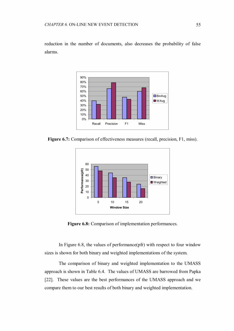
CHAPTER 6. ON-LINE NEW EVENT DETECTION
55
reduction in the number of documents, also decreases the probability of false
alarms.
0%10%20%30%40%50%60%70%80%90%
Recall Precision F1 Miss
BinAvgWAvg
Figure 6.7: Comparison of effectiveness measures (recall, precision, F1, miss).
0
10
20
30
40
50
60
5 10 15 20
Window Size
Perf
orm
ance
(pfr
)
BinaryWeighted
Figure 6.8: Comparison of implementation performances.
In Figure 6.8, the values of performance(pfr) with respect to four window
sizes is shown for both binary and weighted implementations of the system.
The comparison of binary and weighted implementation to the UMASS
approach is shown in Table 6.4. The values of UMASS are barrowed from Papka
[22]. These values are the best performances of the UMASS approach and we
compare them to our best results of both binary and weighted implementation.

CHAPTER 6. ON-LINE NEW EVENT DETECTION
56
System Corpus Miss
%
False Alarm
%
Recall
%
Precision
%
F1
UMASS TDT1 40 1.27 60 52 0.56
Binary TDT1 44 1.27 56 50 0.53 Weighted TDT1 52 0.6 48 63 0.55
Table 6.4: Comparison of on-line new event detection approaches.
In Table 6.4, the UMASS approach has better performance results than our
system, but the UMASS approach gives twice false alarms than our system, when
compared to weighted implementation.
The results of on-line new event detection approaches in TDT study are
shown in Table 6.5. These are the pooled average of 11-pass methodology. Since
only 25 events were judged, this evaluation method is introduced by TDT study in
order to expand the number of trials. But the actual effectiveness values are the
reflection of the task without using 11-pass method. In other words, the actual
system performance is the performance that determined in the 0-pass, without
skiping any document of any event.
System Miss
%
False Alarm
%
Recall
%
Precision
%
F1
UMASS 50 1.34 50 45 0.45
CMU 59 1.43 41 38 0.39 DRAGON 58 3.47 42 21 0.28
Table 6.5: Comparison of systems presented at the first TDT workshop.
In Table 6.5, the UMASS approach has the best results among the other
approaches. Since we do not have the 0-pass values of CMU and DRAGON
approaches, we just compare our system performance to the UMASS approach
values.

57
Chapter 7
Conclusion and Future Work
In this thesis, we implement and evaluate alternative solutions to on-line new
event clustering and on-line event detection problems. The results presented in
this work are based on problem definitions, evaluation methodologies, and data
developed by the topic detection and tracking (TDT) project.
The previous approaches to clustering are usually based on retrospective
solutions, where all the data are available before clustering begins. In order to
find a way to on-line classification, we use the concepts of the C3M algorithm in
an online environment, in which a cluster is determined for the current document
before looking at the next document. For this reason, we introduce an algorithm
that works in a single-pass manner, where the documents are processed
sequentially, one at a time. We use the seed selection process of C3M for
detecting new events. A document detected as new, is also used as the seed of a
cluster. In order to obtain the best performance, we aim to select the initial stories
of the events as seed documents, and group the following stories around the
selected seeds. Furthermore, to prevent producing oversized event clusters, and to
give equal chance to all documents to be the seed of a new event, we employ the
window size concept. The main motivation of this approach is that; documents
closer together on the stream are more likely to discuss similar events than

CHAPTER 7. CONCLUSION AND FUTURE WORK
58
documents further apart on the stream. In our experiments, we aim to see the
impact of different window sizes to the effectiveness results. For this purpose, we
execute the event clustering and on-line new event detection algorithms for each
window. In event clustering experiments, we observe that, the performance
improves with the growing size of window until a point, which is the window size
of 35 (days) in our case. After this point, since the number of documents
increases with the wider window size, the old seeds and the new seeds co-exist in
the same window. Accordingly, the seed documents of the previous events
interfere with the seed documents of the new events. This provides many
different clusters to non-seed documents to join and decreases the system
performance. In event detection experiments, the best window size observed 5.
Different from the event clustering results, we detect that, narrowing the window
increases the performance of the event detection system.
Since we desire to control the number of seed documents, we introduce a
threshold concept to the event clustering algorithm. We also use the threshold
concept, with a little modification, in the on-line new event detection.
We use both binary and weighted versions of TDT1 corpus, and compare
the results of both cases to each other. For the binary case, the system takes the
term frequencies of document vectors (document vectors are created from TDT1,
and they are stemmed and cleaned of stop-words), as binary, in other words if a
particular term exists in the vector, the system takes its term frequency as 1, it is
taken as 0 otherwise. On the contrary, for the weighted implementation, if a term
appears in a document 10 times; its term frequency is taken as 10. Our results
indicate that, for the case of binary event clustering, between 25%-30% of the
documents of the predetermined events are classified by the system correctly. We
obtain better results for binary implementation for event clustering over weighted
case. As an advantage of weighted implementation, the system produces at least
one cluster for each event, which is a desired situation. However, as a side affect,
the number of clusters increases by 10% with respect to the binary version.

CHAPTER 7. CONCLUSION AND FUTURE WORK
59
For the case of on-line new event detection, we use the same concepts that
are used for the event clustering. According to our experimental results for binary
case, we detect between 24%-56% of the documents discussing new events at
relatively low false alarm rates of 0.2%-1.3%. Again, we obtain better results for
the binary implementation, except the precision and false alarm rate. The false
alarm rate of weighted implementation is 54% better than the binary case. This is
because, for the case of binary implementation, system labels more documents as
new. More documents increase the probability of false labels, for example,
system labels a document as new event, when in truth it is not a new event.
Selecting more documents as new, improves the recall value but produces a
weaker false alarm rate.
Different from the event clustering results, in the on-line event detection
case, we observe that narrowing the window size improves the performance of the
system. Using narrower window limits the influence of old seeds to the new
coming events. Since the first seeds have higher seed power values, this affects
the threshold Tr. Accordingly, this high Tr value reduces the chance of new
documents to be selected as a seed. When we use a wider window size, the
effects of these first seeds reach documents, which are quite far away from these
seeds in terms of time. Narrowing the window size decreases the probability of
co-existence of relevant documents with non-relevant ones. This gives more
possibility to new events to be selected as seed.
When we don’t use the window size concept, in the case of event
clustering, the system uses 40% more CPU time, since the number of documents,
processed in a particular window size, is smaller than the whole corpus. We
obtain less number of clusters (33% of the binary implementation with the
window 35) without using window concept. This means that, the first coming
documents, which have higher seed power values, enhance the average seed
power value ( avgP ). This reflects directly to the threshold value (Tr). Since the
system could not eliminate these kinds of documents without determining a
window size, they attract most of the stories in the corpus and construct fat and

CHAPTER 7. CONCLUSION AND FUTURE WORK
60
ineffective clusters. By the help of window size concept, we give equal chance to
each document to be selected as seed. In the case of new event detection, without
using window size concept, we obtain the worst results, which have the
performance (prf) of 8. This is because, without eliminating powerful seed
documents (documents that have high seed power value) from the system, desired
documents cannot exceed the threshold, so that they are not labeled as seed.
Our results are relatively close to the results of TDT study, however, the
accuracy of our approach, even at optimal parameter settings, is far from perfect.
One of the reasons is that, our system is based on the word co-occurrences, which
means that document similarities are computed based on the term similarities.
However, this approach is insufficient for some events. As the event progresses,
many of its properties are either not initially known, or are assumed to be known
by the user, and therefore they are not necessarily clear in news text. For
example, for the event 15, about the earthquake in Kobe, Japan, this referred to
the event as “the worst disaster in Japan’s history,’’ with no explicit mention of
Kobe or the fact that the story was about an earthquake. These kinds of stories
reduce the effectiveness of the system. In order to prevent this, lexical chaining
can be incorporated with our system.
In order to obtain better event clustering and new event detection
accuracy, the same work can be repeated in the retrospective environment, for this
purpose the original C3M algorithm can be used.

61
Bibliography
[1] Allan, J., Incremental Relevance Feedback for Information Filtering, In
Proceedings of ACM SIGIR, 270-278, 1996.
[2] Allan, J., Carbonell, J., Doddington, G., Yamron, J. and Yang, Y., Topic
Detection and Tracking Pilot Study Final Report, In Proceedings of the
DARPA Broadcast News Transcription and Understanding Workshop,
February, 1998.
[3] Allan, J., Ballesteros, L., Callan, J. and Croft, W., Recent Experiments
with Inquery, In Proceedings of TREC-4, pages 49-63, 1995.
[4] Callan, J. Document ltering with Inference Networks, In Proceedings of
the 19th Annual International ACM SIGIR Conference on Research and
Development in Information Retrieval, pages 262-269, 1996.
[5] Callan, J., Croft, W. and Broglio, J., TREC and TIPSTER Experiments
with INQUERY. Information Processing & Management, 31(3):327-343,
1994.
[6] Can, F., On the Efficiency of Best Match Cluster Searches, Information
Processing & Management, Vol.30, No.3, pp. 343-361, 1994.

BIBLIOGRAPHY
62
[7] Can, F. A New Clustering Schema and It’s Use in an Information
Retrieval System Incorporating the Support of a Database Machine, Ph. D.
dissertation, Dept. of Computer Engineering, Middle East Technical
Univ., Ankara, Turkey, 1985.
[8] Can, F. and Ozkarahan, E.A., Concepts and Effectiveness of the Cover
Coefficient-based Clustering Methodology for Text Databases, ACM
Transactions on Database Systems, 15(4): 483-517, 1990.
[9] Can, F. and Ozkarahan, E. A., Effectiveness Assessment of The Cover
Coefficient-based Clustering Methodology, working paper 89-002, Dept.
of System Analysis, Miami Univ., Oxford, Ohio, Oct. 1989.
[10] Can, F. and Ozkarahan, E. A., A Clustering Scheme, In the Proceedings of
the 16 th Annual International ACM-SIGIR Conference. ACM, New York,
1983, pp, 115 – 121.
[11] Carrick, C. and Watters, C., Automatic Association of News Items, Infor-
mation Processing & Management, 33(5): 615-632, 1997.
[12] Croft, W.B., A Model of Cluster Searching Based on Classification,
Information Systems, 5(3): 189-195, 1980.
[13] Croft, W.B., and Harper, D. J., Using Probabilistic Models of Document
Retrieval without Relevance Information, Journal of Documentation, 5(3):
285-295, 1979.
[14] DeJong, G., Prediction and Substantiation: A New Approach to Natural
Language Processing, Cognitive Science, 3: 251-273, 1979.

BIBLIOGRAPHY
63
[15] Goldman, R. P., A Probabilistic Approach to Language Understanding,
Ph.D. Thesis, Brown University, 1990.
[16] Hayes, P.J., Knecht, L.E. and Cellio, M.J., A News Story Categorization
System, In Proceedings of the 2nd Conference on Applied Natural
Language Process (1988), reprinted in Readings in Information Retrieval,
K. Sparck Jones and P. Willet editors, Morgan Kaufmann Publishing, San
Francisco, CA, pp. 518- 526, 1997.
[17] Hodges, J. L. and Lehmann, E. L., Basic Concepts of Probability and
Statistics, Holden Day in San Francisco, CA., 1964.
[18] Hull, D., In Proceedings of Text Retrieval Conferences (TREC6), NIST
Special Publication, pp. 45-67, 1998.
[19] Jain, A. K., Dubes, R. C., Algorithms for Clustering Data, Prentice Hall,
Upper Saddle River, NJ, 1988.
[20] Kurt, H., On-Line New Event Detection and Tracking in A Multi-
Resource Environment, MS. Thesis, Bilkent University, 2001.
[21] Lewis, D. and Gale, W., A Sequential Algorithm for Training Text
Classifiers, In Proceedings of ACM SIGIR, 313, 1994.
[22] Papka, R., On-line New Event Detection, Clustering, and Tracking, Ph. D.
Thesis, University of Massachusetts at Amherst, September 1999.
[23] Proceedings of Message Understanding Conferences, Morgan Kaufmann,
1988.
BIBLIOGRAPHY
64
[24] Proceedings of the TDT Workshop, University of Maryland, College Park,
MD, October 1997 (Unpublished).
[25] Salton, G., Automatic Text Processing: The Transformation, Analysis and
Retrieval of Information by Computer, Reading, MA: Addison-Wesley,
1989.
[26] Salton, G., Dynamic Information and Library Processing, Englewood
Cliffs, NJ: Prentice-Hall, 1975.
[27] Salton, G., Relevance Feedback and Optimization of Retrieval
Effectiveness, in The Smart System - Experiments in Automatic
Document Processing, Prentice -Hall, Englewood Cliffs, N.J., pp. 324-
336, 1971.
[28] Salton, G. and McGill, M.J., Introduction to Modern Information
Retrieval, New York, McGraw-Hill, 1983.
[29] Schank, R., Conceptual Information Processing, Elsevier, North Holland,
New York, 1975.
[30] Sparck, Jones, Karen, and Peter Willet, 1997, Readings in Information
Retrieval, San Francisco: Morgan Kaufmann.
[31] Swets, J., Measuring the Accuracy of Diagnostic Systems, Science,
240:1285-1293, 1988.
[32] The Topic Detection and Tracking (TDT) Pilot Study Evaluation Plan,
Version 2.8, October 97.
BIBLIOGRAPHY
65
[33] van Rijsbergen, C. J., Information retrieval, 2nd ed., London: Butterworths,
1979.
[34] Voorhees, E. M., The Effectiveness and Efficiency of Agglomerative
Hierarchical Clustering in Document Retrieval, Ph. D. Thesis, Cornell
University, Ithaca, NY, 1986.
[35] Walls, F., Jin, H. Sista, S. and Schwartz, R., Topic Detection in Broadcast
News, In Proceedings of the DARPA Broadcast News Workshop, pp. 193-
198, 1999.
[36] Yang, Y., Carbonell, J., Brown, R., Pierce, T., Archibald, B. and Liu, X.,
Learning Approaches for Detecting and Tracking News Events, IEEE
Intelligent Systems, 14(4):32-43, 1999.
[37] Yang, Y., Pierce, T. and Carbonell, J., A Study on Retrospective and On-
Line Event Detection, In Proceedings of the 21st Annual International
ACM SIGIR Conference on Research and Development in Information
Retrieval, pages 28-36, 1998.

66
Appendix
The stop-word list that used for cleaning the TDT1 corpus is given in the sequel.
a about above according across added adding after afterwards again against albeit all almost alone along already also although always am among amongst an and another any anybody anyhow anyone anything anyway
anywhere apart are around as at av b be became because become becomes becoming been before beforehand behind being below beside besides between beyond both but by c can cannot canst certain
cf choose contrariwise cos could cu d day do does doesn doing dost doth double down dual during e each either else elsewhere enough et etc even ever every everybody everyone everything
everywhere except excepted excepting exception exclude excluding exclusive f far farther farthest few ff first for formerly forth forward from front further furthermore furthest g get go h had halves hardly has
hast hath have he hence henceforth her here hereabouts hereafter hereby herein hereto hereupon hers herself him himself hindmost his hither hitherto how however howsoever i ie if in inasmuch inc

APPENDIX
67
include included including indeed indoors inside insomuch instead into inward inwards is it its itself j just k kg kind km l last latter latterly less lest let like little ltd m many may maybe me meantime meanwhile might more moreover most mostly mr mrs ms much must my myself n namely need neither never
nevertheless next no nobody none nonetheless noone nope nor not nothing notwithstanding now nowadays nowhere o of off often ok on once one only onto or other others otherwise ought our ours ourselves out outside over own p per perhaps plenty provide q quite r rather really reuter reuters round s said sake same sang
save saw see seeing seem seemed seeming seems seen seldom selves sent several shalt she should shown sideways since slept slew slung slunk smote so some somebody somehow someone something sometime sometimes somewhat somewhere spake spat spoke spoken sprang sprung stave staves still such supposing t than that the thee their them themselves then thence
thenceforth there thereabout thereabouts thereafter thereby therefore therein thereof thereon thereto thereupon these they this those thou though thrice through throughout thru thus thy thyself till to together too toward towards u ugh unable under underneath unless unlike until up upon upward upwards us use used using v very via vs w want was we
week well were what whatever whatsoever when whence whenever whensoever where whereabouts whereafter whereas whereat whereby wherefore wherefrom wherein whereinto whereof whereon wheresoever whereto whereunto whereupon wherever wherewith whether whew which whichever whichsoever while whilst whither who whoa whoever whole whom whomever whomsoever whose whosoever why will wilt with within without worse worst would wow

APPENDIX
68
x y ye year yet yippee you your yours yourself yourselves z