ON INFORMATION, PRIORS, ECONOMETRICS, AND ECONOMIC MODELING

Francisco Venegas-Martínez Centro de Investigación y Docencia Económicas

Enrique de Alba Instituto Tecnológico Autónomo de México

Manuel Ordorica-Mellado* El Colegio de México

R e s u m e n : Se busca reconciliar aquellos métodos inferenciales que a través de la maximización de una funcional producen dis­tribuciones a p r i o r i no-informativas e informativas. E n particular, las distribuciones a p r i o r i de Evidencia M i n i ­max (Good, 1968), las de Máxima Información de los Datos (Zellner, 1971) y las de Referencia (Bernardo, 1979) son vistas como casos especiales de la maximización de un criterio más general. Bajo un enfoque unificador se presentan las distri­buciones a p r i o r i de Good-Bemardo-Zellner, que aplicamos en varios métodos de inferencia Bayesiana útiles en inves­tigación económica. Asimismo, utilizamos las distribuciones de Good-Bernardo-Zellner en varios modelos económicos.

A b s t r a c t : This paper attempts to reconcile al l inferential methods which by maximiz ing a criterion functional produce n o n -

i n f o r m a t i v e and i n f o r m a t i v e priors. In particular, Good ' s (1968) M in imax Evidence Priors, MEP , Zel lner 's (1971) M a x i m a l Data Information Priors, MDIP, and Bernardo's (1979) Reference Priors, RP, are seen as special cases of maximiz ing a more general criterion functional. In a unify­ing approach Good-Bernardo-Zel lner priors are introduced and applied to a number o f Bayesian inference procedures which are useful i n economic research, such as the Ka lman Filter and the Normal Linear Mode l . W e also use the Good-Bernardo-Zellner distributions in several economic models.

* We are indebted to Arnold Zellner, José M . Bernardo, Jim Berger, George C. Tiao, Manuel Mendoza, and David Mayer for valuable comments and suggestions on earlier drafts of this paper. The authors bear sole responsibility for opinions and errors.

E E c o , 14, 1, 1999 53

54 ESTUDIOS ECONÓMICOS

1. Introduction

The distinctive task in Bayesian analysis of deriving priors so that the inferential content of the data is minimally affected in the posterior distribu­tion, has been of great interest for more than 200 years since the early work of Bayes (1763). More current approaches to this problem, based on the maximization of a specific criterion functional, have been suggested by Good (1969), Zellner (1971) and Bernardo (1979).

When modeling economic systems or conducting empirical research, prior information from previous research or from our knowledge of eco­nomic theory is always available. In either case, the estimates of the pa­rameters of a regression model or the estimates of the time-varying parameters of a state-space model can usually be improved by incorporat­ing any information about the parameters beyond that contained in the sample. In this work, we provide a broad class of priors that are l ikely to be useful in a variety of situations in economic modeling.

The principle of maximum invariantized negative cross-entropy is in­troduced in Good's (1969) minimax evidence method of deriving priors. There, the initial density is taken as the square root of Fisher's information. Zellner (1971) presents, for the first time, a method to obtain priors through the maximization of the t o t a l information about the parameters provided by independent replications of an experiment (prior average information in the data minus the information in the prior). Bernardo (1979) proposed a proce­dure to produce reference priors by maximizing the expected information about the parameters provided by independent replications of an experiment (average information in the posterior minus the information in the prior).

A l l of the above methods have certain advantages: i ) Whi le Zellner's method is based on an exact finite sample criterion

functional, Good's approach uses a l imiting criterion functional, and Ber­nardo's procedure is based on asymptotic results. In Bernardo's proposal a reference prior (posterior) is defined as the limit of a sequence of priors (posteriors) that maximize finite-sample criteria. Many reference prior al­gorithms have been developed in a pragmatic approach in which results are most important. See, for instance, Berger, Bernardo and Mendoza (1989), and Berger and Bernardo (1989), (1992a), (1992b), Bernardo and Smith (1994), and Bernardo and Ramon (1997).

i i ) The criterion functional used by Bernardo is cross-entropy, which satisfies a number of remarkable properties; in particular, it is invariant

ECONOMIC MODELING 55

with respect to one-to-one transformations of the parameters (Lindley, 1956). In contrast, the total information functional employed by Zellner is invariant only for the location-scale family and under linear transforma­tions of the parameters. Addit ional side conditions are needed to generate in variance under more general transformations.

Hi) The way in which these methods have been tested is by seeing how wel l they perform in particular examples.

The evaluation is often based on contrasting the derived priors with Jeffreys' (1961), usually improper, priors which are somewhat arbitrary and inconsistent. In fact, there are cases in which one can strongly recommend avoiding Jeffreys' priors. See, for instance: Box and Tiao (1973), p. 314; Aka ike (1978), p. 58; and Berger and Bernardo (1992a), p. 37.

In this paper, we attempt to reconcile all inferential methods that pro­duce n o n - i n f o r m a t i v e and i n f o r m a t i v e priors. In our unifying approach, M in imax Evidence Priors (Good, 1968 and 1969), Max imal Data Informa­tion Priors (Zellner, 1971, 1977, 1991, 1993, and 1995) and Reference Priors (Bernardo, 1979 and 1996) are seen as special cases of maximizing an indexed criterion functional. Hence, properties of the derived priors wi l l depend on the choice of indexes from a wide range of possibilities, instead of on a few personal points of view with ad h o c modifications. In the spirit of Aka ike (1978) and Smith (1979), we can say that this w i l l look more l ike Mathematics than Psychology —without denigrating the importance of the latter in the Bayesian framework. This unifying approach wi l l enable us to explore a vast range of possibilities for constructing priors. Needless to say, a good choice w i l l depend on the specific characteristics of the problem we are concerned with. It is worthwhile mentioning that our general method extends Soofi's (1994) pyramid in a natural way by adding more vertices and including their convex hull .

This paper is organized as follows. In section 2, we wi l l introduce an indexed family of information functionals. In section 3 we wi l l state a relationship between Bernardo's (1979) criterion functional and some members of the indexed family, on the basis of asymptotic normality. In section 4, we w i l l study a Bayesian inference problem associated with convex combinations of relevant members of the proposed indexed family. Here, we w i l l introduce the Good-Bernardo-Zellner priors and their c o n ­

t r o l l e d versions as solutions to the problem of maximizing discounted entropy. We w i l l pay special attention to the existence and uniqueness of the solution to the corresponding optimization problems. In section 5, we

56 ESTUDIOS ECONÓMICOS

wi l l study the Good-Bernardo-Zellner priors as Kaiman Filtering priors. In section 6, we w i l l apply Good-Bernardo-Zellner priors to the normal linear model, In section 7, we apply Good-Bernardo-Zellner priors to a variety of situations in economic modeling. Finally, in section 8, we present conclu­sions, acknowledge limitations, and make suggestions for future research.

2. An Indexed Family of Information Functionals

In this section, we define an indexed family of information functionals and study some distinguished members. For the sake of simplicity, we w i l l remain in the single parameter case.

Suppose that we wish to make inferences about an unknown parameter 6 6 0 c 1R of a distribution P 9 , from which an observation, say, X , is available. Assume that />e has density/(JC I 9) (Radon-Nikodym derivative) with respect to some fixed dominating a-f inite measure X on 1R for al l 6 e 0 c JR. That is, d P d / d X = f ( x I 9) for all 9 e 0 c 1R and thus P Q ( A )

= J f ( x I Q)dX(x) for all Borel sets A e JR. A The Bayesian approach starts with a prior density, 7t(9), to describe

initial knowledge about the values of the parameter, 9. We w i l l assume that 71(9) is a density with respect to some a-finite measure u on IR. Once a prior distribution has been prescribed, then the information about the pa­rameter provided by the data, x is used to modify the initial knowledge, via B a y e s ' theorem, to obta in a poster ior d i s t r ibut i on of 9, namely, /(9 I x ) «c/(jt I 9)7i(9) for every in JC e IR (We use/generically to represent densities). The normalized posterior distribution is then used to make infer­ences about 9.

Let us define an infinite system of nesting functionals (cf. Venegas-Martinez,1997):

K « . 8 ( 7 t ) = J " ( 6 )0 ( ^ (8 ) . m 7- « , 8 )4 i (9 ) , (2.1)

where

G ( / ( 9 ) , F { Q ) , y, a , 8) =

ECONOMIC MODELING 57

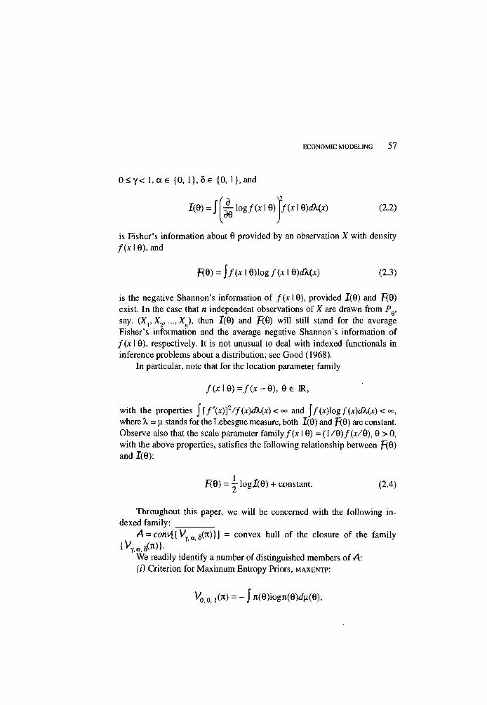
0 < Y < l , a e {0, l } , 8 e {0, l } , and

I ( e ) = J ± l o g f ( X \ Q ) \ f ( x \ Q ) d M x ) (2.2)

is Fisher's information about 9 provided by an observation X with density f ( x I 9), and

is the negative Shannon's information of f ( x I 9), provided 1(9) and R 8 ) exist. In the case that n independent observations of X are drawn from Pg,

say, ( X V X 2 , . . . , X n ) , then 1(9) and F(6) w i l l still stand for the average Fisher's information and the average negative Shannon's information of f ( x I 9), respectively. It is not unusual to deal with indexed functionals in inference problems about a distribution; see Good (1968).

In particular, note that for the location parameter family

with the properties j [ f ' ( x ) ] 2 / f ( x ) d k ( x ) < ~ and j f ( x ) l o g f ( x ) d k ( x ) <

where X. = u. stands for the Lebesgue measure, both 1(9) and R 9 ) are constant. Observe also that the scale parameter f ami l y/ ( * I 9) = (1/9)/(JC/8), 9 > 0, with the above properties, satisfies the following relationship between F(9) and 1(9):

Throughout this paper, we wi l l be concerned with the following in­dexed family:

A = c o n v [ { V y a 5 ( n ) } ] = convex hull of the closure of the family i K , a , 5 ( 7 t ) } .

We readily identify a number of distinguished members of A :

( i ) Criterion for Max imum Entropy Priors, M A X E N T P :

R Q ) = i f ( x \ Q ) l o g f ( x \ Q ) d M x ) (2.3)

/ ( ^ ! 9 ) = / ( x - 9 ) , 9 e IR,

P(6) = y logI(9) +constant. (2.4)

K o . . ( « ) = - J«(e)io gK(e)4i(9),

58 ESTUDIOS ECONÓMICOS

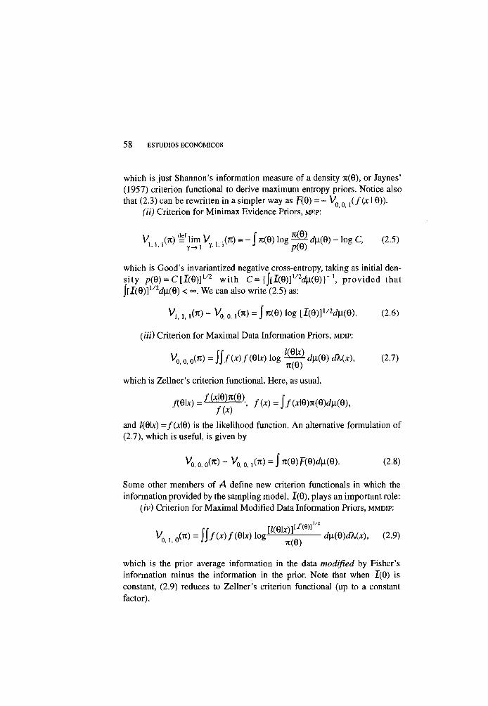
which is just Shannon's information measure of a density jt(6), or Jaynes' (1957) criterion functional to derive maximum entropy priors. Notice also that (2.3) can be rewritten in a simpler way as F(9) = - V Q Q 1 ( f ( x \ 0)).

( i i ) Criterion for M in imax Evidence Priors, MEP :

which is Good's invariantized negative cross-entropy, taking as initial den­s i t y p ( Q ) = C [1(6) ] 1 / 2 w i t h C = { j [ I ( Q ) ] l / 2 d i x ( Q ) r l , p r o v i d e d that j " [ I (0) ] 1 / 24i(9) < oo. We can also write (2.5) as:

K i , i W - K o, i ( « ) = J « ( 6 ) log [i(e)]' / 2^(0). (2.6)

( H i ) Criterion for Max ima l Data Information Priors, MDIP:

V 0 0 0(7t) = j j f ( x ) f ( 0 \ x ) log ^ d i i i Q ) d X ( x ) , (2.7) ' ' 71(9)

which is Zellner's criterion functional. Here, as usual,

f ( e \ X ) =/<*' 9>*( 9 ) , f ( x ) = S f { x \ Q ) n ( e ) d m , f i x )

and /(6bc) = f ( x \ Q ) is the likelihood function. A n alternative formulation of (2.7), which is useful, is given by

K o, o(*) - K o, M ) - i m w ) d m . (2.8)

Some other members of A define new criterion functionals in which the information provided by the sampling model, 1(9), plays an important role:

( i v ) Criterion for Max ima l Modif ied Data Information Priors, MMDIP:

V o , l , o W = [ f / W / W l o g [ / ( e ' ^ ( e ) d m d X ( x ) , (2.9)

which is the prior average information in the data m o d i f i e d by Fisher's information minus the information in the prior. Note that when 1(9) is constant, (2.9) reduces to Zellner's criterion functional (up to a constant factor).

ECONOMIC MODELING 59

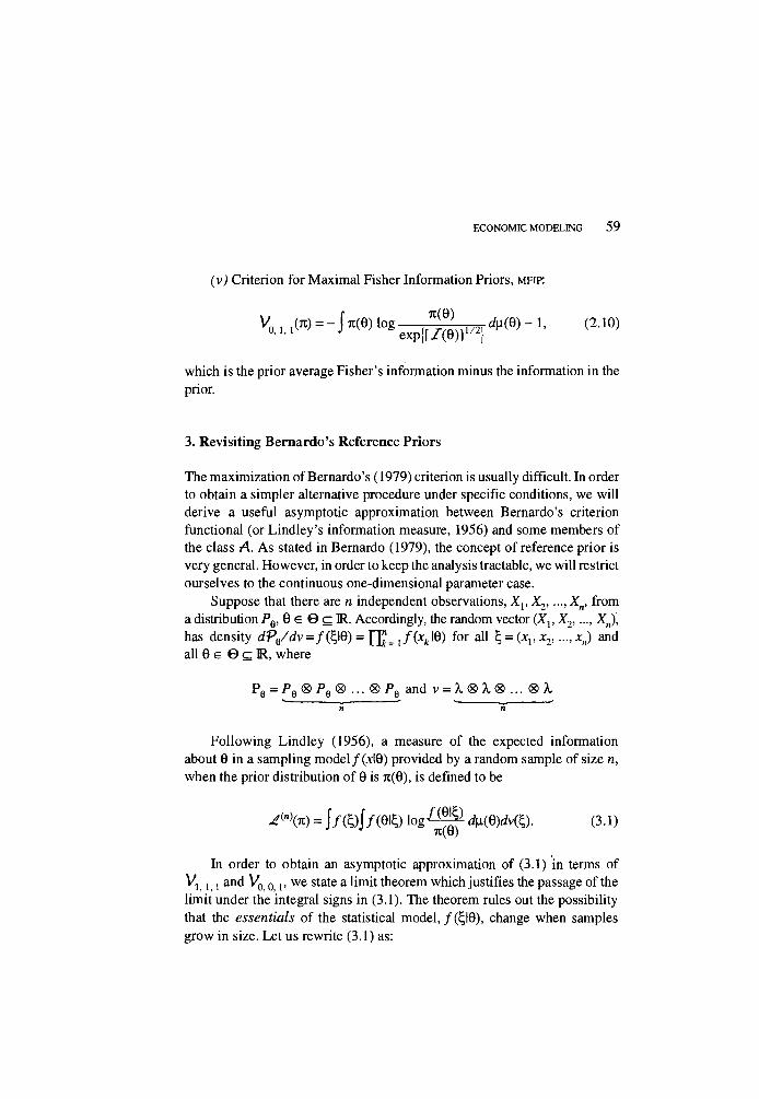
( v ) Criterion for Max ima l Fisher Information Priors, MFIP:

71(0) (2.10)

which is the prior average Fisher's information minus the information in the prior.

3. Revisiting Bernardo's Reference Priors

The maximization of Bernardo's (1979) criterion is usually difficult. In order to obtain a simpler alternative procedure under specific conditions, we w i l l derive a useful asymptotic approximation between Bernardo's criterion functional (or L indley 's information measure, 1956) and some members of the class A . A s stated in Bernardo (1979), the concept of reference prior is very general. However, in order to keep the analysis tractable, we wi l l restrict ourselves to the continuous one-dimensional parameter case.

Suppose that there are n independent observations, X v X 2 , . . . . X n , from a distribution P6, 6 € 0 ç JR. Accordingly, the random vector ( X v X 2 , X n ) ,

has density d P e / d v = / © 9 ) = J { x k \ Q ) for all t, = ( x v x 2 , ...,*„) and all 9 e 0 ç jR, where

P e = P 9 ® P 9 <g> ... <8>Pe and v = \® X® ... ®X

Fo l lowing L ind ley (1956), a measure of the expected information about 9 in a sampling model/^IG) provided by a random sample of size n ,

when the prior distribution of 9 is TC(9), is defined to be

In order to obtain an asymptotic approximation of (3.1) 'in terms of V t l , and V 0 0 v we state a l imit theorem which justifies the passage of the l imit under the integral signs in (3.1). The theorem rules out the possibility that the e s s e n t i a l s of the statistical model, / (£19), change when samples grow in size. Let us rewrite (3.1) as:

~n

• * i n \ n ) - i m i / m l o g ^ ^ d m d v { % ) . 7t(ü)

(3.1)

ECONOMIC MODELING 61

[ ( T (<O)W (co) - T ( e o ) W œ ) £ 0; (3.2) liol > n \^ J

( I X ) T h e s e q u e n c e o f r a n d o m v a r i a b l e s { l o g i / „ }~ = , w h e r e

Un = j r„(co)Wn(co)4i(co) satisfies

l im sup J WogUn\dP = 0, (3.3) e - > ~ n > l Hogt/„l>E

/>{£, e A , 9 e B ] = ¡n(B) \ f (%\Q)dv(\)d\i(Q) (3.4)

f o r a l l A G l R n a n d B G 0 .

77*en, a i n —» °°,

«¿<">(ic) - V , ,(71) = - V 0 o ,((p) + l o g C <n~ + 0(1), (3.5)

wfcere q>(z) ü r te density o/Z ~ W(0, 1), and C is taken as in ( 2 . 4 ) .

Some comments are in order: (I)-(IV) are standard regularity condi­tions, (V) states desirable properties for 1(6), (VI) is a bounded variance condition, (VII) is a smoothness condition, (VIII) is a convergence condi­tion, and (IX) says that the sequence {log <y„}~ =, is uniformly integrable with respect to P.

It can be shown (details can be found in Venegas-Martinez, 1990a) that (I)-(VI) lead to

r„(to) 4 e x p { œ V 7 ( ë ) [ Z - | c o V 7 ( ë ) ] } , (3.6)

where Z ~ N (0, 1), and (3.6) along with (VII)-(IX) imply

log Un = log J rn(co)W„(co)4i(co) 4 log V2TC/7(0) + y Z 2 -

The conclusion of the theorem follows. Note that the right-hand side of (3.5) is independent of 7t. Thus, i f conditions (I)-(LX) are fulfilled, instead of max im i z ing «4M(TC), wh ich is usually dif f icult, we can maximize V , , ,(71), which is independent of « . Note that for maximization purposes the right-hand side of (3.5) becomes a constant.

62 ESTUDIOS ECONÓMICOS

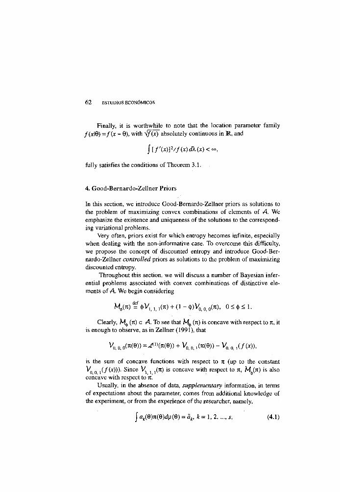
Finally, it is worthwhile to note that the location parameter family f(x\G) = f ( x - 0), with # W absolutely continuous in R , and

In this section, we introduce Good-Bernardo-Zellner priors as solutions to the problem of maximizing convex combinations of elements of A . We emphasize the existence and uniqueness of the solutions to the correspond­ing variational problems.

Very often, priors exist for which entropy becomes infinite, especially when dealing with the non-informative case. To overcome this difficulty, we propose the concept of discounted entropy and introduce Good-Ber­nardo-Zellner c o n t r o l l e d priors as solutions to the problem of maximizing discounted entropy.

Throughout this section, we w i l l discuss a number of Bayesian infer­ential problems associated with convex combinations of distinctive ele­ments of A . We begin considering

Clearly, M,,, (TC) e A . To see that M 0 (TC) is concave with respect to re, it is enough to observe, as in Zellner (1991), that

K o, o f a W ) = ^ H n m + V 0 0 ,(70(9)) - V 0 0 ,(/(*)),

is the sum of concave functions with respect to TC (up to the constant K n ,(/(*))). Since V. . ,(7i) is concave with respect to TC, M.(TC) is also concave with respect to'TC! *

Usually, in the absence of data, s u p p l e m e n t a r y information, in terms of expectations about the parameter, comes from additional knowledge of the experiment, or from the experience of the researcher, namely,

¡[f'(x)]2/f(x)dk(x)<

fully satisfies the conditions of Theorem 3.1.

4. Good-Bernardo-Zellner Priors

def

0 < ¡ , ) V o . ° - o ( 7 t ) '

J a¿(9)7i(6)4i(9) = a k , k = 1, 2 , s , (4.1)

ECONOMIC MODELING 63

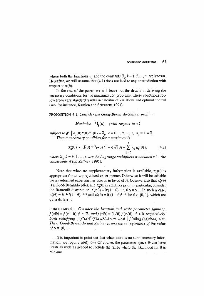
where both the functions a k and the constants a k , k = 1, 2 , s , are known. Hereafter, we w i l l assume that (4.1) does not lead to any contradiction with respect to 7t(6).

In the rest of the paper, we w i l l leave out the details in deriving the necessary conditions for the maximization problems. These conditions fol­low from very standard results in calculus of variations and optimal control (see, for instance, Kamien and Schwartz, 1991).

PROPOSIT ION 4.1. C o n s i d e r t h e G o o d - B e r n a r d o - Z e l l n e r p r o V ' - - :

M a x i m i z e M^TC) ( w i t h r e s p e c t t o i t )

s u b j e c t t o e. f ̂ (6)71(0)41(6) = a^ k ~ 0 , 1, 2, s, a Q = 1 = a Q .

T h e n a n e c e s s a r y c o n d i t i o n f o r a m a x i m u m is

S

rc;(9) - [I (0)]4>/2 e x p { f l - W F ( 0 ) + £ k k a k ( B ) } , (4.2) * = o

w h e r e 1 ^ k = 0, 1, .... s, a r e the L a g r a n g e m u l t i p l i e r s a s s o c i a t e d w / ' h e

c o n s t r a i n t s e ( c f . Z e l l n e r , 1 9 9 5 ) .

Note that when no supplementary information is available, 7^(0) is appropriate for an unprejudiced experimenter. Otherwise it wi l l be suitable for an informed experimenter who is in favor of # Observe also that n*(0) is a Good-Bernardo prior, and 7t*(0) is a Zellner prior. In particular, consider the Bernoull i distribution, '/(jrfG) = 9*(1 - 0) 1 ~ x , 0 < 0 < 1. In such a case, Ti*(6) = e- 1 / 2 (1 - 0 ) ~ I / 2 and iC0(<d) = 0 9(1 - 0 ) ' - e for 6 e [0, 1], which are quite different.

C O R O L L A R Y 4 . 1 . C o n s i d e r the l o c a t i o n a n d s c a l e p a r a m e t e r f a m i l i e s ,

/(xie) = f ( x - 6), 9 e IR, a n d f ( x \ Q ) = ( 1 / Q ) f ( x / Q ) , 6 > 0, r e s p e c t i v e l y ,

b o t h s a t i s f y i n g j [ f ' ( x ) ] 2 / f ( x ) d X ( x ) < o 0 a n d \ f ( x ) \ o g f ( x ) d X ( x ) < ^ .

T h e n , G o o d - B e r n a r d o a n d Z e l l n e r p r i o r s a g r e e r e g a r d l e s s of the v a l u e

o/(j> e (0, 1),

It is important to point out that when there is no supplementary infor­mation, we require u (9 ) < °°. O f course, the parameter space 0 can have limits as wide as needed to include the range where the likelihood for 0 is relevant.

64 ESTUDIOS ECONÓMICOS

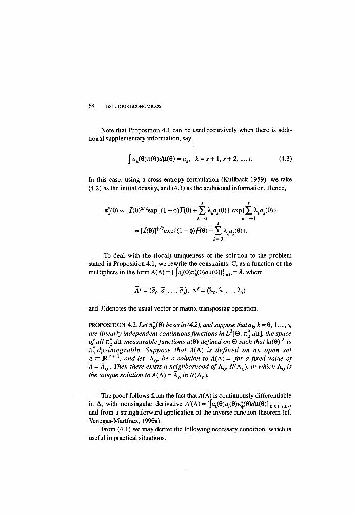
Note that Proposition 4.1 can be used recursively when there is addi­tional supplementary information, say

1^(0)70(0)41(8)=^, k = s + l , s + 2 , . . . , t . (4.3)

In this case, using a cross-entropy formulation (Kullback 1959), we take (4.2) as the initial density, and (4.3) as the additional information. Hence,

TtJiG) - [Key^expUl - <t,)F(G) + £ \ a k ( Q ) } e x p { X X ^ Q ) }

* = 0 k = s + l

= [I(0)]*/ 2exp{(l - <t>)F(8) + £ X A ( 6 ) } . i = 0

To deal with the (local) uniqueness of the solution to the problem stated in Proposition 4.1, we rewrite the constraints, C, as a function of the multipliers in the form A ( A ) = [ |at(0)Tc;(8)4i(8)]^=o = A , where

A T = ( a 0 , a , a,), A T = ( X 0 , X v X s )

and T denotes the usual vector or matrix transposing operation.

PROPOSITION 4.2. L e t TCI(0) be as in (4.2), and suppose t h a t a k , k = 0 , l , s ,

are l i n e a r l y i n d e p e n d e n t c o n t i n u o u s f u n c t i o n s in L 2 [ 0 , n l 41], the space

of a l l TCI d \ i - m e a s u r a b l e f u n c t i o n s a(B) defined on Q such that la (8) l 2 is

7t! d \ i - i n t e g r a b l e . S u p p o s e t h a t A ( A ) is d e f i n e d o n a n o p e n s e t

A <= + l , a n d l e t A 0 , be a s o l u t i o n t o A ( A ) = f o r a fixed v a l u e of

A = A 0 . T h e n t h e r e exists a n e i g h b o r h o o d of A Q , N ( A Q ) , in w h i c h A 0 is

the u n i q u e s o l u t i o n t o A ( A ) = A 0 in N ( A 0 ) .

The proof follows from the fact that A(A) is continuously differentiable in A , with nonsingular derivative A ' ( A ) = [ j a l ( Q ) a l ( Q ) n ^ Q ) d \ l ( Q ) ] o < i ; < s -

and from a straightforward application of the inverse function theorem (cf. Venegas-Martinez, 1990a).

From (4.1) we may derive the following necessary condition, which is useful in practical situations.

ECONOMIC MODELING 65

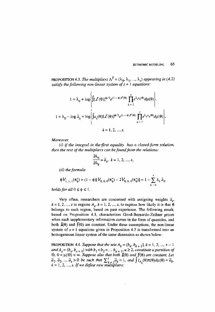
PROPOSIT ION 4.3. T h e m u l t i p l i e r s A T = (X0, X , , X ç ) a p p e a r i n g in ( 4 . 2 )

satisfy t h e f o l l o w i n g n o n - l i n e a r s y s t e m of s + 1 e q u a t i o n s :

\ = X + log

1 = X 0 - l o g ä j f c + log

k = 1

k = 1,2, . . . ,s.

M o r e o v e r ,

( i ) if t h e i n t e g r a l i n t h e first e q u a l i t y h a s a c l o s e d - f o r m s o l u t i o n ,

t h e n t h e r e s t of t h e m u l t i p l i e r s c a n b e f o u n d f r o m t h e r e l a t i o n s :

d X 0

— - = 5 „ ¿ = 1 , 2 , s, d X k

k

( i i ) t h e f o r m u l a

S

<t>K. !, + o - •)[ v 0 , o, <,(*;> - 2 K o, i ( « p ] = 1 - X \ % k = Q

h o l d s f o r a l l O < $ < 1.

Very often, researchers are concerned with assigning weights d k ,

k = \ , 2 , s to regions A k , k = 1 , 2 , s , to express how likely it is that 6 belongs to each region, based on past experience. The following result, based on Proposition 4.3, characterizes Good-Bernardo-Zellner priors when such supplementary information comes in the form of quantiles, and both 1(6) and F(6) are constant. Under these assumptions, the non-linear system of s + 1 equations given in Proposition 4.3 is transformed into an homogeneous linear system of the same dimension as shown below:

PROPOSITION 4.4. Suppose t h a t the sets A k = ( b k , b k + ,], k = 1, 2, s - 1 a n d A s = ( b s , b s + x ) w i t h b l < b 2 < ... b u + v u > 2 , c o n s t i t u t e a p a r t i t i o n of

9 , 0 < (1(0) < oo. Suppose a l s o t h a t b o t h 1(6) a n d f { Q ) a r e c o n s t a n t . L e t

a v a 2 , d s > 0 b e s u c h t h a t ^ a k = 1, a n d \ l A (6)71(6)^(6) = a h

¿ = 1 , 2 , s. If we define n e w m u l t i p l i e r s : "

66 ESTUDIOS ECONÓMICOS

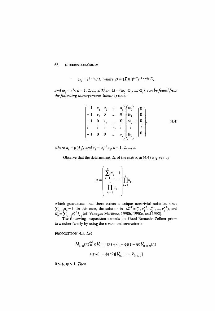
©„ = e 1 " V D where D = [ 1 ( 0 ) ] ^ ^ ~ •>»»,

and w k = e\ k = \ , 2 , . . . , s . Then, Q. = ( (0 Q , co,, m) can be f o u n d f r o m

the f o l l o w i n g h o m o g e n e o u s l i n e a r system:

- 1 " l u 2 . s

f \

0 ( 0 )

- 1 0 . . 0 0), 0

- 1 0 . 0 = 0

- 1 0 0 V (Ú 0 V S

J V J l J

(4.4)

where u k = \ i { A k ) , and vk = a ~ l u k , k = l , 2, s.

Observe that the determinant, A, of the matrix in (4.4) is given by

A : X V 1

*= i

*=i

n « *=i

which guarantees that there exists a unique nontrivial solution since J H = l a k = l . In this case, the solution is (1, \ v~2 v ; ' ) , and K = Tl= A ' 7 A ( c f Venegas-Martinez, 1990b, 1990c, and 1992).

The fol lowing proposition extends the Good-Bernardo-Zellner priors to a richer family by using the MMDIP and MFIP criteria:

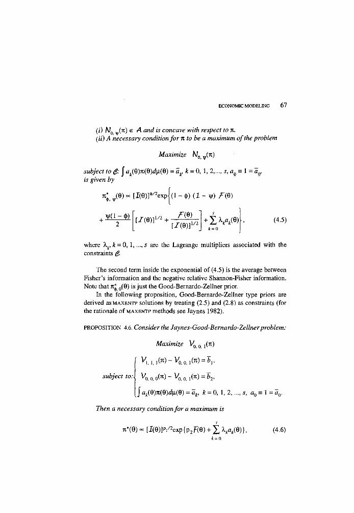
PROPOSIT ION 4.5. L e t

\ V(TC)=F 4) V , , ,(TC) + (1 - 0X1 - V ) V 0 0 0(7C)

+ ( V ( i - < t » / 2 ) [ V 0 , , + y 0 1 0 ]

0<<j>, \\i< 1. Then

ECONOMIC MODELING 67

( i ) (TC) e A a n d is c o n c a v e with r e s p e c t t o %.

( i i ) A n e c e s s a r y c o n d i t i o n f o r n t o be a m a x i m u m of the p r o b l e m

M a x i m i z e

s u b j e c t t o & \ ^(6)71(6)41(6) = a^ k = 0, 1, 2,..., s, a Q s 1 = a f f

is g i v e n by

n l , v ( 6 ) 0 0 [KSW^exp j i l - d)) (1 - v|/) f ( 6 )

2 1/2

1/2 * = 0

(4.5)

where \ , k = 0,1,.... J are the Lagrange multipliers associated with the constraints £

The second term inside the exponential of (4.5) is the average between Fisher's information and the negative relative Shannon-Fisher information. Note that TCJ 0(6) is just the Good-Bernardo-Zellner prior.

In the fol lowing proposition, Good-Bernardo-Zellner type priors are derived as M A X E N T P solutions by treating (2.5) and (2.8) as constraints (for the rationale of M A X E N T P methods see Jaynes 1982).

PROPOSIT ION 4.6. C o n s i d e r the J a y n e s - G o o d - B e r n a r d o - Z e l l n e r p r o b l e m :

M a x i m i z e V 0 0 ,(7t)

s u b j e c t t o : . V 0 0 0(TC) - V 0 0 ,(TC) = b 2 ,

1^(0)71(6)41(6) = ^ , t = 0, 1,2,..., j , a0s\=â0.

T h e n a n e c e s s a r y c o n d i t i o n f o r a m a x i m u m is

71*0) « tI(6)]P/ 2exp{p 2F(6) + X V * ( e ) } > k = 0

(4.6)

68 ESTUDIOS ECONÓMICOS

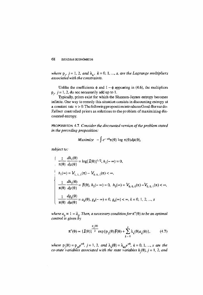
where p., j = 1, 2, a n d \ , k = 0, 1, s, a r e t h e L a g r a n g e m u l t i p l i e r s

a s s o c i a t e d with t h e c o n s t r a i n t s .

Unl ike the coefficients 4» and 1 - « ) appearing in (4.6), the multipliers p j y j = 1, 2, do not necessarily add up to 1.

Typically, priors exist for which the Shannon-Jaynes entropy becomes infinite. One way to remedy this situation consists in discounting entropy at a constant rate v > O.Thefol lowingproposit ionintroducesGood-Bernardo-Zel lner control led pr iors as solutions to the problem of max imiz ing dis­counted entropy.

PROPOSIT ION 4.7. C o n s i d e r the d i s c o u n t e d v e r s i o n of the p r o b l e m s t a t e d

in the p r e c e d i n g p r o p o s i t i o n :

M a x i m i z e - j e~ V6TC(9) log 7t(9)4t(9),

s u b j e c t t o :

i d h , ( Q )

Ai(°°> = K , , , ( « ) - M>, o,i

' 1 d h J Q ) = F(9), h J - °°) = 0, hJ°°) = Vn n n(rc) - V n n A n ) < °°,

7t(9) 4i(9) 2 2 ° ' a o ° ' a i

1 d g k ( Q ) — = a d d ) , gt(- °°) = 0, g.(°o) < oo, jfc = 0, 1, 2, s

7t(9) du(9) * S k S k

where a Q s 1 = a . T h e n , a n e c e s s a r y c o n d i t i o n f o r 7t*(9) t o be an o p t i m a l

c o n t r o l is g i v e n by

P,W

TC*(9) - [1(G)] 2 exp{p 2 (9)F(6) + X y 9 ) a t ( 9 ) } , (4.7) * = o

wrtere p.(9) = p . 0 e v 9 , j = 1 , 2 , a n d X m = X^e™, k = 0, 1 j are the

c o - s t a t e ' v a r i a b l e s a s s o c i a t e d with the state v a r i a b l e s h ( Q ) , j = 1, 2, a n d

ECONOMIC MODELING 69

g ( Q ) , k = 0 , \ , s, respectively. F u r t h e r m o r e , the constants p.Q, j = 1, 2, a n d X , k = 0, 1, s can be c o m p u t e d f r o m the f o l l o w i n g n o n - l i n e a r

system o f s + 3 e q u a t i o n s :

1 + log «,(oo) =

log{J log[I(e)F 2m(p 1 0 ) p m J ^ , X 1 0 , . . . . X J 0 ; 6)41(6)},

1 + log n2(oo) •= l og j j R 6 ) m ( p 1 0 > p 2 Q , X m , \ Q , X s Q , 6)4i(8)},

1 + log g k M = log {Ja t(9 )m(p 1 0, p 2 0 , A^,, X 1 0 , X j 0 ; 8)4i(8)},

¿ = 0 , 1 , 2, j ,

where

« ( p . o . p20. V ^10. 0 ) = f [ iW] 2 e p » R 9 ) * H I A o ° " ( e ) • u= 1 '

5. Kalman Filtering Priors

In this section, we wi l l study Good-Bernardo-Zellner priors as Kalman Filtering priors (Kalman 1960, and Kalman and Bucy 1961). We w i l l continue to work with the single parameter case, and focus our attention on the location parameter family.

Let Yv Y2,Yt be a set of indirect measurements, from a poll ing system or a sample survey, of an unobserved state variable ft. The objective is to make inferences about ft. The relationship between Yt and ft is specified by the measurement or observation equation:

y t = A f f t + e f, (5.1)

where A ( * 0 is known , and £, is the observation error distributed as W(0, 0 2) with a 2 known. Note that the main difference between the mea­surement equation and the linear model is that, in the former, the coefficient ft changes with time. Furthermore, we suppose that ft is driven by a first order autoregressive process, that is,

70 ESTUDIOS ECONÓMICOS

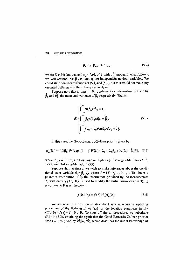
p > Z , p ( _ , + ! ! , _ „ (5.2)

where Z * 0 is known, and x\ ~ N ( 0 , a1) with o 2 known. In what follows, we wil l 'assume that p e,, and n ( are^ndependent random variables. We could state nonlinear versions of (5!l) and (5.2), but this would not make any essential difference in the subsequent analysis.

Suppose now that at time t = 0, supplementary information is given by P 0 and a 2 , the mean and variance of p 0 respectively. That is,

J TC(P 0 ) r fp 0 =l ,

J _ P 0 T C ( P o ) d P 0 = P 0 ,

f ( P 0 - P 0 ) 2 T C ( p 0 ) dp 0 = O 2 .

(5.3)

In this case, the Good-Bernardo-Zellner prior is given by

rc;(p 0) * [ I (p 0 ) ] * / 2 e x p { ( l - <b)F(Po) + \ + M o + M P o " Po) 2 } ' (5-4>

where X., j = 0, 1, 2, are Lagrange multipliers (cf. Venegas-Martinez e t a l ,

1995, and Ordorica-Mellado, 1995). Suppose that, at time t, we wish to make inferences about the condi­

tional state variable e,= P tl/ t, where /,= { Y v Y2 K f_,}. To obtain a posterior distribution of 6,, the information provided by the measurement Yr with density/(F, I 0 r), is used to modify the init ial knowledge in TC*(0,) according to Bayes ' theorem:

/(0,1 Y t ) o c f ( Y t I e,)TC*,(0,). (5.5)

We are now in a position to state the Bayesian recursive updating procedure of the Kalman Filter (KF) for the location parameter family / ( y , l 0 ) = / ( y , - 0 ) , 0 e R . To start off the K F procedure, we substitute (5.4) in (5.3), obtaining the result that the Good-Bernardo-Zellner prior at time t = 0, is given by /v(p0, a 2 ) , which describes the initial knowledge of

ECONOMIC MODELING 71

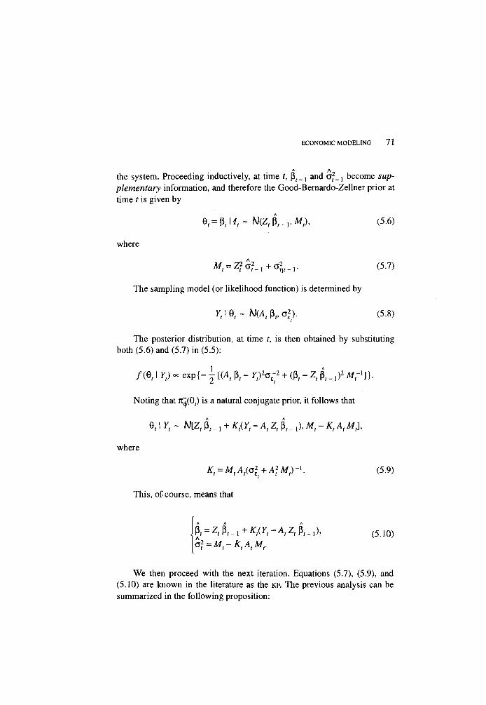
the system. Proceeding inductively, at time f, p , _ , and a j _ , become sup­

p l e m e n t a r y information, and therefore the Good-Bernardo-Zellner prior at time t is given by

e,= f j , l/ , ~ N (Z,p\-p M t ) , (5.6)

where

M l ^ Z j a 2 _ l +0-2,,.,. (5.7)

The sampling model (or l ikelihood function) is determined by

y, I 9 ( ~ N ( A , p f , o 2 ) . (5.8)

The posterior distribution, at time t, is then obtained by substituting both (5.6) and (5.7) in (5.5):

/(9,1 Yt) - exp {- j [(A, p r - Y t ) 2 o ~2 + (p, - Z ( p\ _ , ) 2 A/ ~>]}.

Not ing that TCJ(0() is a natural conjugate prior, it follows that

Qt\Yt~ N [ Z , p,_ , + ^ ( l 7 , - A , Z, p,_ ,), Af f - K t A , M t ] ,

where

Af, = A * , A r ( a 2 + A 2 M t ) ~ K (5.9)

This, of course, means that

. P r - Z / P r - l + ^ M - A Z f P f - l ) ' (5.10) a 2 = M t - A : ( A ( M ( .

We then proceed with the next iteration. Equations (5.7), (5.9), and (5.10) are known in the literature as the KF . The previous analysis can be summarized in the following proposition:

72 ESTUDIOS ECONÓMICOS

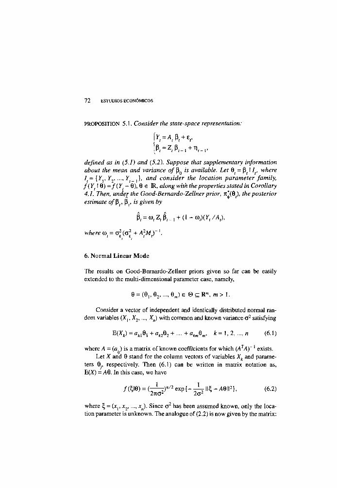
PROPOSIT ION 5.1. C o n s i d e r the s t a t e - s p a c e r e p r e s e n t a t i o n :

|P, = Z , P , _ ,

defined as in ( 5 . 1 ) a n d ( 5 . 2 ) . S u p p o s e t h a t s u p p l e m e n t a r y i n f o r m a t i o n

a b o u t the m e a n a n d v a r i a n c e of P Q is a v a i l a b l e . L e t 9 = 0 I / (, w h e r e

I , = { Y V Yv .... F ,}, a n d c o n s i d e r t h e l o c a t i o n p a r a m e t e r f a m i l y ,

f ( Y I 9) = f ( Y - 9), 9 e R, a/ong wi in ifte p r o p e r t i e s s t a t e d in C o r o l l a r y

4 . 1 . T h e n , u n d e r t h e G o o d - B e r n a r d o - Z e l l n e r p r i o r , n \ ( B ) , the p o s t e r i o r

e s t i m a t e o/P ( , P,, is g i v e n by

P, = a>,Z, p , _ , + ( l -(û,)(Yt/At),

w h e r e co, = a 2 ( a 2 + A 2 M ) ~ \ t t

6. Normal Linear Mode

The results on Good-Bernardo-Zellner priors given so far can be easily extended to the multi-dimensional parameter case, namely,

9 = ( 8 , , 9 2 , 0 J e 8 c R " , m > 1.

Consider a vector of independent and identically distributed normal ran­dom variables (X,, X 2 , X n ) with common and known variance o 2 satisfying

E ( X k ) = a H e i + a k 2 6 2 + . . . + a k m Q m , * = 1 , 2 , n (6.1)

where A = ( a . ) is a matrix of known coefficients for which ( A T A ) ~ 1 exists. Let X and 9 stand for the column vectors of variables X k and parame­

ters 6,, respectively. Then (6.1) can be written in matrix notation as, E(X) = A B . In this case, we have

= ( ^ z " ) " 7 2 e xp { - ll£ - A9II 2 }, (6.2)

where £ = ( x v x 2 , x n ) . Since a 2 has been assumed known, only the loca­tion parameter is unknown. The analogue of (2.2) is now given by the matrix:

ECONOMIC MODELING 73

TT-tog/(jtl6) a e , l o g / ( A r l e ) f ( x \ B ) d \ ( x )

A < 1,1 < m

= -hATA (6.3)

and so det[I (9)] is constant.which implies that the Good-Bernardo-Zellner prior distribution TC'O), describing a situation of vague information on 9, must be ajocally uniform prior distribution.

Let 9 be the least squares estimate for 9. Then it is known that A T A Q = A T X , E(9) = 9, and Var (9) = a 2 { A T A ) ~ l. Noting from equation (6.2) that

/ ( § 6 ) : ( 1 ^ 2

2TCG2

V J

2 e x p { - ~~~ (ll£ - A9II 2 + ( A T A ( Q - 9), 9 - 9 ))}, 2 a 2

and applying Bayes' theorem, we get as the posterior distribution of 9

m i ' i i /(9I£) = ( 2 n ) ~ 2 ( d e t [ ^ A T A ] ) H x p { - \ ( \ A T A { Q - 9), 9 - 9 )}.

If supplementary information about the mean, c, and the variance-co-variance matrix, D , is now incorporated, then the (informative) Good-Ber­nardo-Zellner prior is given by

n'Aß) = (2rc)" 2(det[Z>])~2 exp { - j { D ~ \ Q - c), 0 - c ) } .

The posterior distribution is now

/(9l£) = (27i)"T(det[S])2

x exp {- \ < B[9 - ( ( D B ) ^ c + ^ B ~ l A T A Q ) ] 0

( ( D B ) - i c + J - B - , A T A Q ) ) } , a 2

w h e r e ß ^ D - ' + ^ j A 7 ) ! .

74 ESTUDIOS ECONÓMICOS

7. Good-Bernardo-Zellner Priors in Economic Modeling

In this section we apply Good-Bernardo-Zellner priors to a variety of situations in economic modeling.

E x a m p l e 7.1

Let us examine the behavior of an individual who learns about the parame­ters of her/his utility function under inflation. If we think of the parameters as random variables, then the information gained from experience (con­sumption) is incorporated into a prior distribution. Once a prior is available, the agent makes consumption decisions. To illustrate this process, we shall borrow some ideas from Calvo (1986). Let us consider a small open econ­omy with a single infinitely-lived consumer in a world with a single perish­able consumption good. Suppose that the good is freely traded, and its domestic price level, P , is determined by the purchasing power parity condition, namely P = P * E , where P* is the foreign-currency price of the good, and E is the nominal'exchange'rate. Throughout the paper, we w i l l assume, for the sake of simplicity, that P* is equal to 1. We also assume that the exchange-rate initial value, E , 'is known and equal to 1.

The expected utility function of a representative individual at the pre­sent, t = 0, has the following separable form:

V = f \ f u { c t ; Q ) e - n d L ( Q ) d Q (7.1)

where « ( c ; 6) is the utility of consumption; cf is consumption; 6 > 0 is a parameter related to the utility index; r is the subjective rate of discount; rc(9) is a prior distribution describing initial knowledge of 6 coming from the experience of the consumer before t = 0 (the present).

Let us assume that: 1) the representative individual has perfect fore­sight of the inflation rate so P/P, = q = qe, that is, she/he accurately per­ceives the rate at which inflation is proceeding, the value P(0) is assumed to be known, 2) there are no barriers to free trade, 3) the international interest rate is equal to r, 4) capital mobility is perfect. If i is the nominal interest rate then r = i + qe. Denoting income and government lump-sum transfers by y t

and g t respectively, we can write the consumer's budget constraint, at time / = 0, as

ECONOMIC MODELING 75

«o + l (y + g , ) e - " d t = \ ( c . + i m t ) e - r ' d t , (7.2) 0 0

where for the sake of simplicity we have chosen y ; = y = constant. The con­sumer holds two assets: cash balances, m = M / P , where M is the nominal

t t t t stock of money; and an international bond, £ . The bond pays a constant interest rate r (i.e., pays r units of the consumption good per unit of time). Thus, the consumer's wealth, a f is defined by

a t = m t + k t , (7.3)

where a Q is exogenously determined. Furthermore, we suppose that the rest of the world does not hold domestic currency.

Consider a cash-in-advance constraint of the Clower-Lucas-Feenstra form, m t > etc,, where c, is consumption, and a > 0 is the time that money must be held to finance consumption. Given that i > 0, the cash-in-advance constraint w i l l hold with equality,

m , = a c , (7.4)

For the sake of concreteness, let us suppose that u(ct\ 8) = - e~9c.

Plainly, u c > 0 and u c c < 0. Moreover, let us assume that there is supplemen­tary information about 6 > 0 in terms of the mean value E[8] = l / X . We also assume that 1(8) and F(9) are constant, i.e., before supplementary information becomes available, initial knowledge is vague. In such a case, fol lowing Proposition 4.1, the Good-Bernardo-Zellner prior is given by TC*(8) = e" x e , 8 > 0, and (7.1) can be written as

V=r\f-e-^ + ^ d d ] e r t d t = f - ( - V l f r ' d t . (7.5) Jo [Jo J Jo ct + X

In maximiz ing (7.5) subject to (7.2) the first-order condition for an interior solution is:

1 = X ( \ + a i ) , (7.6) ( c + X)

where X is the Lagrange multiplier associated with (7.2).We assume a government budget constraint of the form

76 ESTUDIOS ECONÓMICOS

f g . e - " d t = b 0 + \ ( m t + q m , ) e - r < d t , (7.7) 0 0

where b denotes the government's holding of international bonds. Let us denote by/ the total bond holding of the economy, i.e., /= k { + b . Then by (7.2) and (7.7) we get

/ 0 + f y e - r ' d t = \ c . e - r ' d t . (7.8) o o

Suppose that expected inflation (depreciation) takes the values q\ in [0, T ] and q\ in (T, °°), where T > 0 and q\ < q\. Since X is time-invariant, we have

A / l + q ( r ^ t T c 2 = A c i + X ( A - l ) , 0 < A = \ \ + a { r + q l ) < l <7-9)

where c, is consumption in [0, T ] and c 2 is consumption in (T, «>).

O n the other hand, from (7.8), we obtain

which leads to

c2 = (y + r f 0 ) e r T + c , ( l - e r T ) (7.11)

The perfect foresight equilibrium consistent with the consumer's opti­mal decisions and government behavior is the intersection point, ( c p c 2), between (7.9) and (7.11). Observe that, in (7.9), a once-and-for-all increase in X, which results in a decrease in the mean value, E[8] = 1/X, w i l l decrease the value of the intercept, X(A - 1), which in turn increases c,. In other words, X reinforces the effect of the rate of time preference. Thus, an increase in X

causes a rise in present consumption and a fall in future consumption.

Other possibilities of supplementary information, using the notation in (4.1), are listed below. In some cases, however, it might only be possible to analyze the equilibrium via numerical methods.

( i ) If a,(9) = 161 and 5, = cx, c t>0, then the Good-Bernardo-Zellner prior is

1 —i-101 K * ( Q ) = — e « ,

2 a

ECONOMIC MODELING 77

which is a Laplace distribution. ( i i ) If

k ( 9 ) = e

k(e)=* e and

ä = - - + ß , ß e 1R a

ä, = « p T ( l + - ) 2 a

where K is Euler 's constant, then TC*(8) = c x e ^ - ^ e x p } - e a ( f l -P' } , which is a Gumbel (or extreme value) distribution.

( H i ) If

W9> fl,(9)

a 2 (0) = 9

a 3(9) = log9

and

« , = 1

5 2 = | , - a > 0 , ß > 0

a 3 = \|/(a)-logP

where7 is the usual indicator function and, as before, V|/(ct) is the p r i

function, then TC*(9) = ^ (P6) a " 1 pe " p e , which is a Gamma distribution

(or Erlang distribution, i f a is a positive integer). ( i v ) If

a 2 (9) = eP, p > 0 [ and

fl,(6) = log9

äj = 1

ä, = - , a > 0 2 a

- K log a p ß

where K is Euler 's constant, then TC*(9) = a P 9 p ~ V 0 * , which'is a Weibull distribution.

E x a m p l e 7.2

We wi l l develop Good-Bernardo-Zellner interval estimates to test conver­gence of rational expectations. Consider a simple macroeconomic model

ECONOMIC MODELING 79

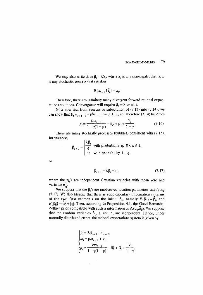
We may also write ft as ft = X \ where x , is any martingale, that is, x

is any stochastic process that satisfies

E { x l + l \ I , ) = x r

Therefore, there are infinitely many divergent forward rational expec­tations solutions. Convergence w i l l require ft = 0 for all t.

Note now that from successive substitution of (7.13) into (7.14), we can show that E , m t + j _ x = p/'m, _ = 0, 1 , a n d therefore (7.14) becomes

p m , _ , _ g - + p V ; _ 6

1 - 7 ( 1 - P) K ' 1 - Y

There are many stochastic processes (bubbles) consistent with (7.15), for instance,

P\+i

X f t — with probabi l i ty q, 0 < q < 1,

q 0 with probabi l i ty 1 - q,

or

ft+1 = Xf t + r i ( , (7.17)

where the TI/S are independent Gaussian variables with mean zero and variance a 2 .

We suppose that the ft's are unobserved location parameters satisfying (7.17). We also assume that there is supplementary information in terms of the two first moments on the in i t ia l (30, namely £{|30}=P0 and £{p2} =o2+ pg. Then, according to Proposition 4.1, the Good-Bernardo-Zellner prior compatible with such a information is N ( % , c 2 ) . We suppose that the random variables p0, e ( and r\, are independent. Hence, under normally distributed errors, the rational expectations system is given by

ft^ft^+Tl,.,,

p m ' ~ ' - 5 - | Q I V ' P l 1 - 7 ( 1 - p) y P i 1-y'

80 ESTUDIOS ECONÓMICOS

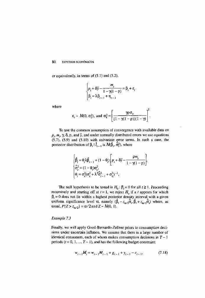
or equivalent^, in terms of (5.1) and (5.2),

m

1 - 7 ( 1 - p )

where -|2

e, ~ N(0, a 2 ) , and a 2 = y p o v

[1 - 7 ( 1 - P ) ] ( l - 7 )

To test the common assumption of convergence with available data on p t , m,, y, 5, p, and y, and under normally distributed errors we use equations (5.7), (5.9) and (5.10) with univariate error terms. In such a case, the posterior distribution of p, 11,_ , is N(P,, a 2 ) , where

CT(2 = ( l - e f ) a 2 ,

The null hypothesis to be tested is H 0 : p > 0 for all t > 1. Proceeding recursively and starting off at f = 1, we reject H 0 i f a f appears for which P, = 0 does not lie within a highest posterior density interval with a given uniform significance level a , namely (p, - Z a / 2 O t , P, + Z a / 2 c r ( ) where, as usual, P { Z > Z a / 1 ) = a / 2 and Z ~ \/(0, 1).

Finally, we w i l l apply Good-Bernardo-Zellner priors to consumption deci­sions under uncertain inflation. We assume that there is a large number of identical consumers, each of whom makes consumption decisions in T- 1 periods (f = 0, 1 , T - 1), and has the following budget constraint:

p^G^P^j+O-e, ) p + S y -1 -7 (1 - p ) '

w t _ x M t = w t _ x M t _ , + g , _ l + y , _ l - ct_l, (7.18)

ECONOMIC MODELING 81

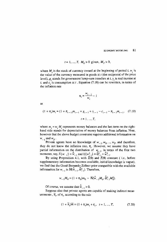
t = 1, T, M 0 > 0 g iven, M T > 0 ,

where M f is the stock of currency owned at the beginning of period r, w ( is the value of the currency measured in goods at t (the reciprocal of the price level), gt stands for government lump-sum transfers at t, y t is real income at t, and c 'is consumption at t. Equation (7.18) can be rewritten, in terms of the inflation rate

as

"t-1 . 71, = 1

(1 +7t ( )m, = ( l +TC,_ , ) « , _ , + y , _ , - c , _ , - n f _ , / « , _ , , (7.19)

i = 1, r ,

where m ( = w f M ( represents money balances and the last term on the right-hand side stands for depreciation of money balances from inflation. Note, however that the above budget constraint requires additional information on w_ and w T .

Private agents have no knowledge of w _ p w Q , w r and therefore, they do not know the inflation rate, n t . However, we assume they have partial information on the distribution of w _ v in terms of the first two moments, say, E{ w_,} = w _ , and E{w2_,} = a l , + w 2 _ , .

B y using Proposition 4.1, with 1(9) and F(9) constant ( i.e., before supplementary information becomes available, initial knowledge is vague), we find that the Good-Bernardo-Zellner prior compatible with the available information for w_ , is N ( w _ , , & ,). Therefore,

w_ i M 0 = (1 + 7t 0 )m 0 ~ W(w_ X M 0 , a 2 . X M 2 ) .

Of course, we assume that vv_, > 0. Suppose also that private agents are capable of making indirect meas­

urements , 7t,, of 7tr, according to the rule

(1 +7C f)m = ( l + 7 t ( ) m , + £,, t = l , . . . , T , (7.20)

82 ESTUDIOS ECONÓMICOS

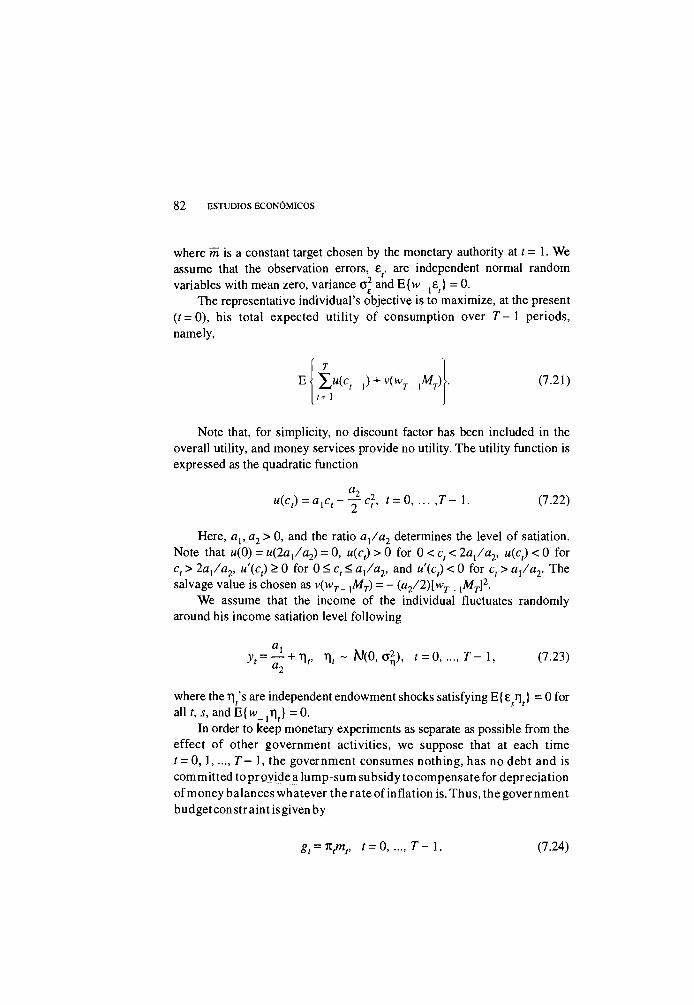
where m is a constant target chosen by the monetary authority at t = 1. We assume that the observation errors, e, are independent normal random variables with mean zero, variance a 2 and E{w_ ,£ (} = 0.

The representative individual's objective is" to maximize, at the present (f = 0), his total expected uti l i ty of consumption over T-\ periods, namely,

(7.21)

Note that, for simplicity, no discount factor has been included in the overall utility, and money services provide no utility. The utility function is expressed as the quadratic function

u ( c t ) = a l C t - ^ c l t = 0,...,T-\. (7.22)

Here, a v a 2 > 0, and the ratio a / a 2 determines the level of satiation. Note that « (0) = u ( 2 a / a 2 ) = 0, u ( c ) > 0 for 0 < c, < 2 a / a 2 , u ( c , ) < 0 for c, > 2 a / a 2 , u ' ( c , ) > 0 for 0 < c, < a / a 2 , and u { c ) < 0 for c, > a / a 2 . The salvage value is chosen as v (w r _ X M T ) = - ( a 2 / 2 ) [ w T _ , M T ] 2 .

We assume that the income of the individual fluctuates randomly around his income satiation level following

V f = f i + T i f , Ti, ~ AJ(0, a 2 ) , t = 0,...,T-\, (7.23)

where the n ' s are independent endowment shocks satisfying E{e r\} = 0 for a l l f , j , a n d E { W _ I T i < } = 0 .

In order to keep monetary experiments as separate as possible from the effect of other government activities, we suppose that at each time f = 0 , 1 , T - 1, the government consumes nothing, has no debt and is committed to pr ovide a lump-sum subsidy to compensate for depreciation of money balances whatever the rate of inflation is. Thus , the gover nment budget constr aint is given by

g , = n / n p i = 0 T - 1. (7.24)

ECONOMIC MODELING 83

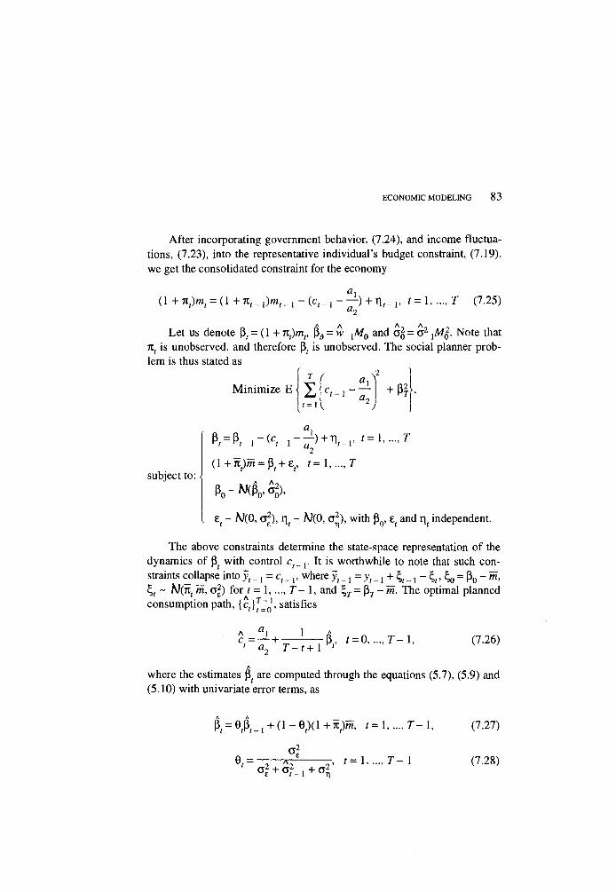
After incorporating government behavior, (7.24), and income fluctua­tions, (7.23), into the representative individual's budget constraint, (7.19), we get the consolidated constraint for the economy

( l + n t ) m t = ( l + n t _ l ) m t _ l - ( c t _ l - ^ - ) + T\t_l, r = 1, T (7.25)

Let us denote ft = (1 + n t ) m r ft, = H>_ ,A/0 and a 2 = a 2 XM%. Note that

n, is unobserved, and therefore ft is unobserved. The social planner prob­lem is thus stated as

M i n i m i z e E + ß2-

P t = P, i - ( c < i L) + r'/ v t = l , . . . , T

( l +Tc )m = ft+e 1 = 1 , . . . , T subject to: <|

P o ~ W ( P o ^ o ) '

e ; ~ N/(0, a 2 ) , r\t ~ N ( 0 , a 2 ) , with (3Q, e ( and r i ( independent.

The above constraints determine the state-space representation of the dynamics of ft with control ct_x. It is worthwhile to note that such con­straints collapse into y , _ x = c t _ x , where y t _ x = y t . x + ^ t _ x - 4 0 = Po ~ »». ^ ~ W(TC;m, o 2 ) for t = 1 , 7 - 1, and £ r = P r - m . The optimal planned consumption path, { c , ) ^ t satisfies

c = — + P , / = 0. t = o , r - 1 , (7.26)

where the estimates ft are computed through the equations (5.7), (5.9) and (5.10) with univariate error terms, as

ft = G ( f t _ , + ( ! - 9 ^ ( 1 + ^ » 1 , /=!,..., 7 - 1 , (7.27)

, /=!, . . . , 7 - 1 (7.28)

84 ESTUDIOS ECONÓMICOS

ö 2 = ( l - 6 ( ) C T 2 , f = l , . . . , T - l (7.29)

Moreover, the optimal salvage value is reached at

ß r = 0 r ß r _ , + (1 - e r ) ( l + n r ) m > 0.

8. Summary and Conclusions

We have presented, in a unifying framework, a number of wel l-known methods that maximize a criterion functional to obtain non-informative and informative priors. Our general procedure is, by itself, capable of dealing with a range of interesting issues in Bayesian analysis. However, in this paper, we have limited our attention to Good-Bernardo-Zellner priors as well as their application to Bayesian inference.

The choice of a prior distribution depends on experience and knowl­edge. Thus, it is impossible to choose a prior that w i l l always be applicable to all circumstances. In our approach the Good-Bernardo-Zellner priors provide a broad class of prior distributions that are appropiate for use in a variety of situations in economic theory and applied econometrics.

Throughout the paper, we have emphasized the existence and unique­ness of the solutions to the corresponding variational and optimal control problems. There are, of course, many other members of the class A that deserve much more attention than what we have attempted here. Needless to say, more work w i l l be required in this direction. Results w i l l be reported in future work.

References

Aka ike , H . (1978). " A New Look at the Bayes Procedure" , B i o m e t r i k a , no. 65, pp. 53-59.

Bayes, T. (1763). " A n Essay Towards So lv ing a Problem in the Doctrine o f Chan­ces " , reprinted in B i o m e t r i k a (1958). no. 45, pp. 243-315.

Berger, J . O. and J . M . Bernardo (1992a). " O n the Development o f Reference P r i o r s " , in J . M . Bernardo e t a/.(eds.), B a y e s i a n S t a t i s t i c s , no. 4, pp. 35-60.

( 1992b). " Ordered Group Reference Priors with Appl icat ion to a Mul t inomia l P r ob l em" , B i o m e t r i k a , no. 79, pp. 25-37.

(1989). "Es t imat ing a Product o f Means: Bayesian Analys is with Reference Pr i o r s " , Journal of the A m e r i c a n Statistical A s s o c i a t i o n , no. 84, pp. 200-207.

ECONOMIC MODELING 85

and M . Mendoza (1989). " O n Priors that Max im i z e Expected Informat ion" , i n J . K l e i n and J . Lee (eds.), R e c e n t D e v e l o p m e n t s i n S t a t i s t i c s a n d t h e i r

A p p l i c a t i o n s , pp. 1-20. Bernardo, J . M . (1996). "Noninformat ive Priors Do Not Exist : A D i s cuss i on " ,

J o u r n a l of S t a t i s t i c a l P l a n n i n g a n d I n f e r e n c e .

(1979). "Reference Posterior Distributions for Bayesian Inference", J o u r n a l

o f t h e R o y a l S t a t i s t i c a l S o c i e t y , B 4 1 , pp. 113-147. and J . M . Ramón (1997). A n I n t r o d u c t i o n t o B a y e s i a n R e f e r e n c e A n a l y s i s :

I n f e r e n c e o n t h e R a t i o o f M u l t i n o m i a l P a r a m e t e r s , Tech. Rep. 3-97, Univer ­sität de Valenc ia , Spain.

and A . F . M . Smith (1994). B a y e s i a n T h e o r y , John Wi l ey & Sons, W i l e y Series in Probabil i ty and Mathematical Statistics.

B o x , G . E . P. and G . C . T iao (1973). B a y e s i a n I n f e r e n c e a n d S t a t i s t i c a l A n a l y s i s ,

Addison-Wesley Series i n Behavioral Science, Quantitative Methods. Ca lvo , G . A . (1986). "Temporary Stabilization: Predetermined Exchange Rates " ,

J o u r n a l of P o l i t i c a l E c o n o m y , no. 94, pp. 1319-1329. Good , I. J . (1969). " W h a t is the Use of a Distr ibut ion?" , Krishnaiah (ed.), M u l t i v a ­

riate A n a l y s i s , V o l . IT, New York , Academic Press, pp. 183-203. (1968). " U t i l i t y o f a D is t r ibut ion" , A t o r e , no. 219.

Jaynes, E . T. (1982). O n t h e R a t i o n a l e of M a x i m u m - E n t r o p y M e t h o d s , Procedures of the I E E E , no. 70, pp. 939-952.

(1957). " Information Theory and Statistical Mechan i cs " , P h y s i c a l R e v i e w ,

no. 106, pp. 620-630. Jeffreys, H . (1961). T h e o r y of P r o b a b i l i t y , 3rd. edition, Oxford University Press. Ka iman, R. E . and R. Buey (1961). " N e w Results in Linear Fi l tering and Prediction

Theory " , T r a n s a c t i o n s A S M E , S e r i e s D. J. of B a s i c E n g i n e e r i n g , no. 83, pp. 95-108.

Ka iman, R. E . (1960). " A New Approach to Linear Fi l tering and Prediction Pro­b l ems " , T r a n s a c t i o n s A S M E , S e r i e s D. J. of B a s i c E n g i n e e r i n g , no. 82, pp. 35-45. .

Kamien , M . I. and N . L . Schwartz (1991). D y n a m i c O p t i m i z a t i o n , the C a l c u l u s of

V a r i a t i o n s a n d O p t i m a l C o n t r o l i n E c o n o m i c s a n d M a n a g e m e n t , 2nd. edi­tion, Amsterdam, North Hol land.

Ku l lback , S. (1959). I n f o r m a t i o n T h e o r y a n d S t a t i s t i c s , New York , John Wi l ey & Sons.

L ind ley , D . V . (1956). " O n a Measure of Information Provided by an Exper iment " , A n n a l s of M a t h e m a t i c a l S t a t i s t i c s , no. 27, pp. 986-1005.

Ordor ica-Mel lado, M . (1995). E l F i l t r o d e K a i m a n en laplaneación demográfica,

Ph. D . Dissertation, Department of Operations Research, Engineering Graduate School , U N A M .

Smith, C . A . B . (1979). "D i s cuss i on of Professor Bernardo's paper", J o u r n a l o f t h e

R o y a l S t a t i s t i c a l S o c i e t y , B 4 1 , p p . 134-135. S o o f i . E . S. (1994). "Cap tur ing the Intangible Concept of Information", J o u r n a l of

t h e A m e r i c a n S t a t i s t i c a l A s s o c i a t i o n , no. 89, pp. 1243-1254.

86 ESTUDIOS ECONOMICOS

Venegas-Martínez, F. (1997). O n I n f o r m a t i o n F u n c t i o n a l a n d P r i o r s , M e m o r i a del X I I Foro Nac ional de Estadística, Asociación Mex icana de Estadística, INEGI, pp. 183-188.

(1992). "En t ropy Max imiza t ion and Cross-Entropy Min imiza t ion : A Matr ix A p p r o a c h " , A g r o c i e n c i a , Serie Matemáticas Aplicadas, Estadística y C o m p u ­tación, pp. 71-77.

(1990a). " O n Regularity and Optimality Condit ions for M a x i m u m Entropy P r i o r s " , T h e B r a z i l i a n J o u r n a l o f P r o b a b i l i t y a n d S t a t i s t i c s , no. 4, pp. 105-136.

(1990b). "Información suplementaria a pr ion , aspectos c o m p u t a c i o n e s y clasificación'' Estadística, Interamerican Statistical Institute, no. 42, pp. 64-80.

, . 1 9 9 0 C )J " I n [ o r m a c , o n , suplementaria a pr ion C o n t r i b u t i o n s t o Prob­

a b i l i t y a n d M a t h e m a t i c a l S t a t i s t i c s , Acts of the IV Lat in-Amencan Meet ing

\ R de A ba and M . Ordonca-Mel lado (1995 . A n Economist s Gu.de to the Ka iman Fi l ter , E s t u d i o s Económicos, E l Coleg io de Mex i co , vo l . 1U, no. 2,

•7,, P P l 2 n o o 5 , w . o t , D . p i . „ . , n t I f f- p . „ Zel lner, A . ( 995). Past and Recent Results on Max ima l Data Informat.on Pnors ,

G r Ä f i DS M E S T ' f

U n l v et

r s l t y o f C h l c a ë ° (manuscnp ). (1993). Mode s Pr ior Informat.on and Bayes.an Analys is , presented at

the Conference on Informat.onal Aspects o f Bayes.an Stat.st.cs in Honor o f H .

Akfinn'A° " & p e a r m \TÍm\1SSU! £ f T k e ÍT of Econometrics. (1991). "Bayes .an Methods and Entropy in Economics and E c o n o m i c s ,

i n W . T. Grandy and L . H . Schick (eds.), M a x i m u m E n t r o p y a n d B a y e s i a n

M e t h o d s , Netherlands, K luwer , pp. 17-31. „ (1977). " M a x . m a l Data Informat.on Pnor D.stnbuüons", m A . A y k a c and

C . B ruma l (eds.), N e w D e v e l o p m e n t s i n t h e A p p l i c a t i o n o f B a y e s i a n M e t h o d s ,

Amsterdam, North-Hol land, pp. 201-232. (1971). A n I n t r o d u c t i o n t o B a y e s i a n I n f e r e n c e i n E c o n o m e t r i c s , New

York , John Wi l ey & Sons.