On including travel time reliability of road traffic in ... · The standard deviation, variance, range, percentiles and derived measures such as buffer index3 fall into this group

1

On including travel time reliability of road traffic in appraisal Gerard C. de Jonga,b,* and Michiel C.J. Bliemerc a Significance, The Netherlands b Institute for Transport Studies, University of Leeds, UK c Institute of Transport and Logistics Studies, The University of Sydney Business School, Australia * Corresponding author at: Significance, Koninginnegracht 23, 2514 AB The Hague, The Netherlands. Tel.:+31-70-3121533. Email address: [email protected] (G. de Jong).

mailto:[email protected]

2

Abstract In many countries, decision-making on proposals for national or regional infrastructure projects in passenger and freight transport includes carrying out a cost-benefit analysis for these projects. Reductions in travel times are usually a key benefit. However, if a project also reduces the variability of travel time, travellers, freight operators and shippers will enjoy additional benefits, the ‘reliability benefits’. Until now, these benefits are usually not included in the cost-benefit analysis. To include reliability of travel or transport time in the cost-benefit analysis of infrastructure projects not only monetary values of reliability, but also reliability forecasting models are needed. As a result of an extensive feasibility study carried out for the German Federal Ministry of Transport, Building, and Urban Development this paper aims to provide a literature overview and outcomes of an expert panel on how best to calculate and monetise reliability benefits, synthesised into recommendations for implementing travel time reliability into existing transport models in the short, medium, and long term. The paper focuses on road transport, which has also been the topic for most of the available literature on modelling and valuing transport time reliability.

Keywords: travel time reliability, travel time variability, road traffic, appraisal

3

1. Introduction

The valuation of travel time reliability (also called: value of variability, VOR) has been receiving considerable attention in recent years, in freight and especially in passenger transport. The main motivation behind this focus on the VOR lies in the desire to include travel time variability in cost-benefit analyses (CBA) of transport projects and policies. But for inclusion of variability in CBA, not only VORs are needed, but also models/methods that predict the impact of infrastructure projects and other transport policies on travel time variability as well as models/methods that predict the likely behavioural responses of travellers, shippers and carriers to changes in travel time variability (as part of the transport models that are used to provide the transport inputs to the CBA).

It has been widely recognised that travellers do not only take travel time into account, but also travel time reliability. In the presence of travel time unreliability, travellers typically allow more time (headstart) for their trips in order to reduce the possibility of arriving late at their destination. Reducing the unreliability (in other words, increasing the travel time reliability) means that this extra time allowance could be decreased or avoided completely, presenting a clear user benefit. It has been argued that travel time unreliability costs are of about the same magnitude as travel time costs. Therefore, in project appraisal there may not only be user benefits in terms of travel time savings, but also in terms of travel time unreliability. By not including travel time reliability in CBA an important user benefit may be discarded, which may result in different project rankings or infrastructure not being built while including reliability benefits could mean a benefit-cost ratio above one. As such, inclusion of travel time reliability is important for assessing projects and policies.

Governments from all over the world are currently considering including travel time reliability benefits in project appraisal. At this moment, only few countries (such as Australia and New Zealand) have included travel time reliability explicitly in CBA. In various other countries (including the UK, the US, Sweden, Denmark, the Netherlands and Germany) policy makers and researchers have started to work on these topics. This paper provides an international review of studies on forecasting travel time variability. Some of these postulate a relation between variability and travel time, others establish a variability-flow relation (similar to a speed-flow relation), controlling for factors such as seasonal variation, weather, road works, accidents, road geometry and traffic management. Besides a review of the literature, this paper also presents practical recommendations at different levels of complexity and effort on how to include reliability in project appraisal. Forecasting travel (or transport) time variability is important for both road and rail transport (potentially also for waterways transport). However, so far almost all the studies on this topic have been dealing with road transport only, and in our review of the literature we necessarily follow the same tracks. Furthermore, almost all literature on forecasting models for road travel time reliability does not distinguish between passenger cars, buses and freight transport vehicles (because a lack of reliable data to make these distinctions).

This paper is based on a project carried out for the German Federal Ministry of Transport, Building and Urban Development (BMVBS)1. The research question was whether and how reliability in road, rail and inland waterways transport could be integrated into the cost-benefit analysis (CBA) of Federal Transport Infrastructure Plan in Germany (BVWP). In this paper, we will be looking at the wider issue how reliability can be included in any country’s project appraisal in the short, medium and long run, generalising the lessons learned for the German case whenever possible. The project looked at passenger and freight transport and focussed on reliability of travel (transport) time, and included an extensive review of the national and international literature, interviews with decision-makers in freight transport and interviews to collect expert opinions (from 21 teams/individuals across the world). A key event was an expert workshop on including reliability in project appraisal

1 Now called the German Federal Ministry of Transport and Digital Infrastructure (BMVDI).

4

that took place on 29 November 2011 in Berlin, with 27 participants from Germany, the UK, the Netherlands, Sweden, Norway and the US.

This paper will focus on day-to-day travel time variations instead of with-in day variations. The day-to-day variations (i.e., variations in travel time when departing at the same time each day) are typically most of interest, as this is the uncertainty that travellers and shippers predominantly have to deal with.

Including travel time reliability in the CBA involves three issues, namely (i) deriving a monetary value of reliability: the value of reliability (VOR), (ii) incorporating the reaction of infrastructure users in passenger and freight transport to reliability in transport forecasting models, and (iii) forecasting the impact of infrastructure projects on reliability. In the Netherlands (e.g. Significance et al., 2013), the first one is typically referred to as the P-side (P of price), and the last two refer to the Q-side (Q of quantity). In the CBA for reliability benefits, in the end one multiplies P with Q. In the UK (e.g. Bates, 2010), a different distinction is made, namely the first two issues are combined into demand issues, and the third one is considered a supply issue. In this paper we will use the terms P- and Q-side.

In Section 2 we discuss which operational definition of reliability is most appropriate for including reliability in CBA. The literature on the VOR has been reviewed in a few recent papers. Therefore, our treatment of the P-side will be very brief (Section 3). In Section 4 we then describe the experiences in developing forecasting models and in forecasting methods for the impact of infrastructure projects of reliability in a number of countries (issues (ii) and (iii) mentioned above). Recommendations for the inclusion of reliability in project appraisal are presented in Section 5, and finally Section 6 gives a summary and conclusions.

2. Travel time reliability definitions and measures

2.1 Two groups of operational definitions

Many definitions of reliability of travel time or transport time2 are used in the literature. We are specifically looking for an operational definition that is appropriate for use in CBA (and in the transport models that provide inputs to the CBA).

In general, two main groups of commonly used operational definitions of reliability can be found in the literature. The first one defines reliability as a measure of dispersion of the travel time distribution. The standard deviation, variance, range, percentiles and derived measures such as buffer index3 fall into this group. This leads to the ‘mean-dispersion’ model 4, which in its simplest form is defined as (taking the standard deviation as the dispersion measure):

RTC TCU [1]

where U is the utility, βC is the cost coefficient (to be estimated), C is the travel or transport cost, βT is the time coefficient (to be estimated), T is the travel or transport time, βR is the reliability coefficient (to be estimated), is the standard deviation of the travel or transport time distribution and is the disturbance term. The value of time (VOT, also referred to as the value of travel time

2 We use travel time for passenger travel and transport time for freight transport.

3 The Buffer-Index is the percentage share of additional travel time that a traveller has to leave earlier than on

average in order to still be on time in 95% of the cases: (T95-M)/M, where T95 is the 95th percentile of the travel time distribution and M is the mean travel time.

4 In the literature this is often called the ‘mean-variance’ model. We use ‘mean-dispersion’ here, since in

practice most models use the mean and another measure of the dispersion than the variance, such as the standard deviation.

5

savings, VTTS) may be defined as the marginal rate of substitution between travel time and travel cost in the above utility function. It can be calculated by dividing the time coefficient by the cost coefficient, i.e. ./ CTVOT The value of reliability (the marginal rate of substitution between reliability and cost) is calculated in a similar way, namely ./ CRVOR

The second group defines schedule delay. Following the equilibrium scheduling model of Vickrey (1969) and Small (1982), the scheduling consequences of reliability are expressed as the expectation on the number of minutes one arrives (or departs) earlier or later than one’s preferred arrival (departure) time.. The Vickrey/Small utility function has the following form:

LateEarlyTCU LateEarlyTC [2]

where βEarly is the coefficient on early arrival (to be estimated), Early is the Schedule delay early (in number of minutes earlier than preferred), βLate is the coefficient on late arrival (to be estimated), and Late is the schedule delay late (in number of minutes later than preferred).5 The value of

schedule delay early (VOSDEarly) and late (VOSDLate) can be calculated as CEarlyVOSDEarly /

and ./ CLateVOSDLate

There is a theoretical equivalence relation (under certain assumptions) between the Vickrey/Small scheduling approach (after taking expectations) and an approach using the mean and the standard deviation of travel time (Bates et al, 2001; Fosgerau and Karlström, 2010).6. Therefore, it is theoretically possible to calculate a dispersion measure (and hence a VOR) from a departure time choice model. The best approach will depend on how one can obtain the best empirical data and which model would fit best in the transport forecasting model system that is used (Börjesson et al., 2012).

In principle, it is possible to estimate both a coefficient on the standard deviation (or variance) and on the schedule delay terms. Such a utility function looks like:

LateEarlyTCU LateEarlyRTC [3]

In practice, it is often difficult to find significant coefficients for both βR as well as for βEarly and βLate (Hollander, 2006; Carrion and Levinson, 2012), though some authors have been able to estimate all such parameters within a single model (e.g. Tseng, 2008; Arellana et al., 2012) Note that the interpretation of the VOR derived from a pure mean-dispersion model might be different from the interpretation of the VOR from the combined model, since all scheduling costs in [1] might be included in the VOR, whereas they are not all captured by the VOR derived from [3]. Studies that investigated the equivalence between the scheduling approach and the mean-dispersion approach using empirical data found a substantial difference in the numerical outcomes between both approaches (Börjesson et al., 2012).

Defining reliability also means defining punctuality and robustness. We define punctuality as deviations from the published timetable (so this is only relevant for public transport) and robustness

5 To account for uncertain travel time, expectations of all terms should be taken, as in Bates et al. (2001).

6 A related alternative scheduling model was presented by Vickrey (1973) and re-introduced by Tseng and

Verhoef (2008). This model starts from the time-varying utility of time spent at the origin and the destination location. Fosgerau and Engelson (2011) have shown that with random travel time (independent of departure time), the optimal expected utility in this model depends only on the mean and the variance of travel time. They derived basically the same result for scheduled services. This implies that there is also an equivalence relation between the Vickrey/Tseng/Verhoef scheduling model and a model with the mean and the variance of travel time.

6

as what happens in the case of calamities (extreme events; so this refers to the far right-hand side tail of the travel time distribution).

2.2 The experts’ choice

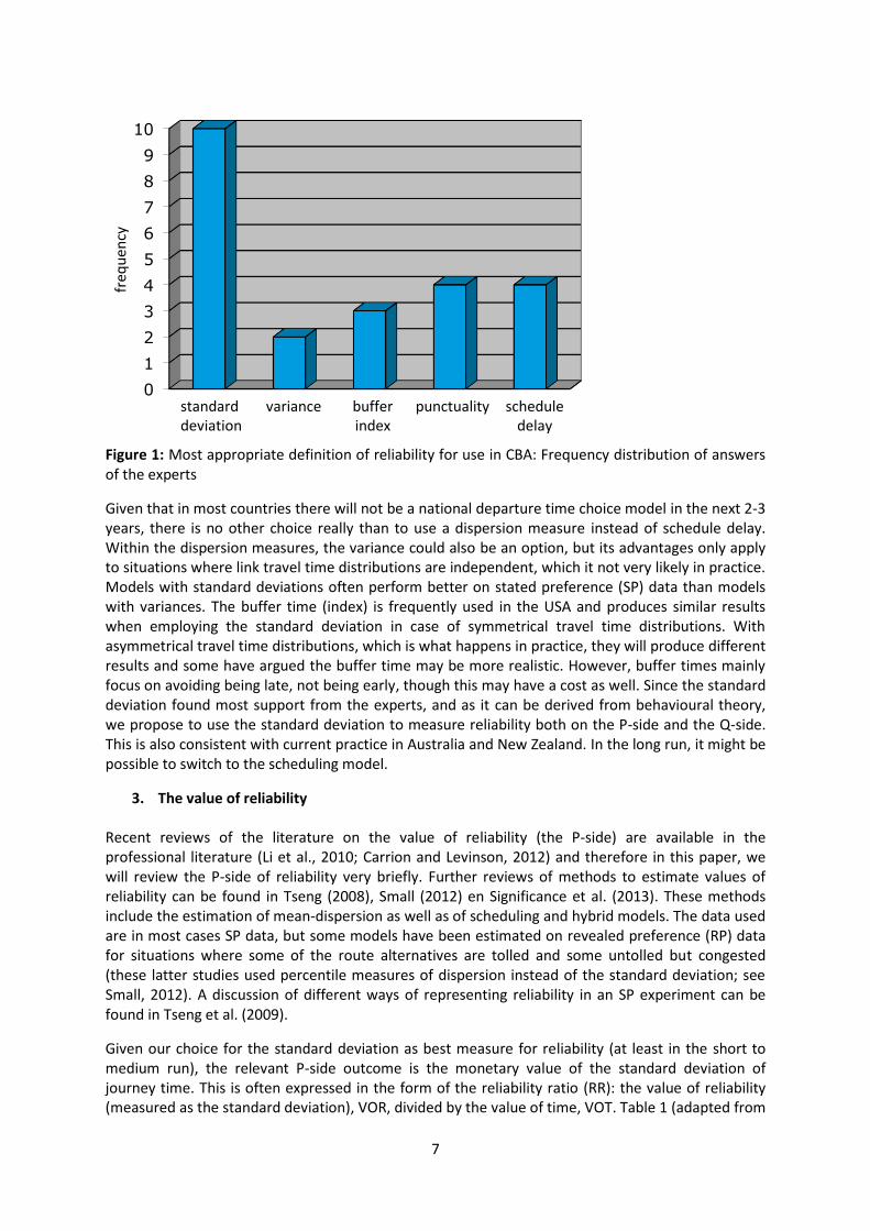
We interviewed international experts7 on travel and transport time reliability. One of the questions was which operational definition of reliability they would recommend for including reliability in the CBA in the next 2-3 years (in the context of Germany, that has federal transport models which do not include scheduling models of the type discussed above; but this is true of almost every national or regional transport model used across the world for appraisal). Below is a chart of the frequency distribution of the answers of the experts. From Figure 1 it is very clear that the standard deviation has most support among the experts as a measure of reliability that can be included in the CBA in 2-3 years from now.

2.3 Proposed use of the standard deviation, arguments for and against

We also reviewed the literature on arguments for and against different operational definition and asked the experts to give their arguments for and against. With respect to the standard deviation we obtained the following arguments.8 Arguments for using the standard deviation are: (i) it has an indirect base in theory, since Fosgerau and Karlström (2010) showed the formal equivalence with the scheduling model (at least for modes without timetables, such as the car), (ii) it can be empirically measured, (iii) it is relatively easy to include in standard transport models (since it does not require including a scheduling model to the transport model, but only an extra reliability term in choices like mode and route choice), (iv) related to the previous, since it requires no formal scheduling model, it also does not require preferred arrival times (PATs), for which specific survey interviews would be needed or reverse engineering (Kristoffersson, 2011), (v) it often provides a good fit to stated preference (SP) data (choices between alternatives that differ in terms of reliability are often well explained by a model that includes the standard deviation), (vi) it can capture a residual (non-scheduling-related) value (e.g. anxiety), (vii) it is a natural way to summarise a distribution (together with the mean). Arguments against using the standard deviation are: (i) it is rather sensitive to outliers, (ii) it is dependent on other aspects (such as other moments) of the travel time distribution, though it does not properly pick up the form of the tail and skew, (iii) it is not additive over links: even when link travel times are independent of each other, simple summation of standard deviations (unlike the variance) over links will not give the standard deviation of the route that uses these links. Choosing variance may resolve the last argument, however, in a congested network, congestion spreads backwards from the original bottleneck, creating dependence among the travel times of adjacent links. In this situation, the variance is not additive over links either.

7 John Bates, Richard Batley, Maria Börjesson, Jonas Eliasson, Leonid Engelson, Mogens Fosgerau, Tony

Fowkes, Joel Franklin, Justin Geistefeldt, Askill Halse, Bruce Hellinga, David Hensher, Yaron Hollander, Juergen Janssen, Anders Karlström, Paul Koster, Hao Li, Tim Lomax, Hani Mahmassani, Rich Margiotta, Kai Nagel, Juan de Dios Ortúzar Salas, Stefanie Peer, John Polak, Farideh Ramjerdi, Piet Rietveld, Henrik Swahn, Lori Tavasszy, Erik Verhoef, Inge Vierth, Peter Vovsha, Tom van Vuren, Mark Wardman, Pim Warffemius.

8 Arguments for and against other measures can be found in Significance et al. (2012).

7

Figure 1: Most appropriate definition of reliability for use in CBA: Frequency distribution of answers of the experts

Given that in most countries there will not be a national departure time choice model in the next 2-3 years, there is no other choice really than to use a dispersion measure instead of schedule delay. Within the dispersion measures, the variance could also be an option, but its advantages only apply to situations where link travel time distributions are independent, which it not very likely in practice. Models with standard deviations often perform better on stated preference (SP) data than models with variances. The buffer time (index) is frequently used in the USA and produces similar results when employing the standard deviation in case of symmetrical travel time distributions. With asymmetrical travel time distributions, which is what happens in practice, they will produce different results and some have argued the buffer time may be more realistic. However, buffer times mainly focus on avoiding being late, not being early, though this may have a cost as well. Since the standard deviation found most support from the experts, and as it can be derived from behavioural theory, we propose to use the standard deviation to measure reliability both on the P-side and the Q-side. This is also consistent with current practice in Australia and New Zealand. In the long run, it might be possible to switch to the scheduling model.

3. The value of reliability Recent reviews of the literature on the value of reliability (the P-side) are available in the professional literature (Li et al., 2010; Carrion and Levinson, 2012) and therefore in this paper, we will review the P-side of reliability very briefly. Further reviews of methods to estimate values of reliability can be found in Tseng (2008), Small (2012) en Significance et al. (2013). These methods include the estimation of mean-dispersion as well as of scheduling and hybrid models. The data used are in most cases SP data, but some models have been estimated on revealed preference (RP) data for situations where some of the route alternatives are tolled and some untolled but congested (these latter studies used percentile measures of dispersion instead of the standard deviation; see Small, 2012). A discussion of different ways of representing reliability in an SP experiment can be found in Tseng et al. (2009).

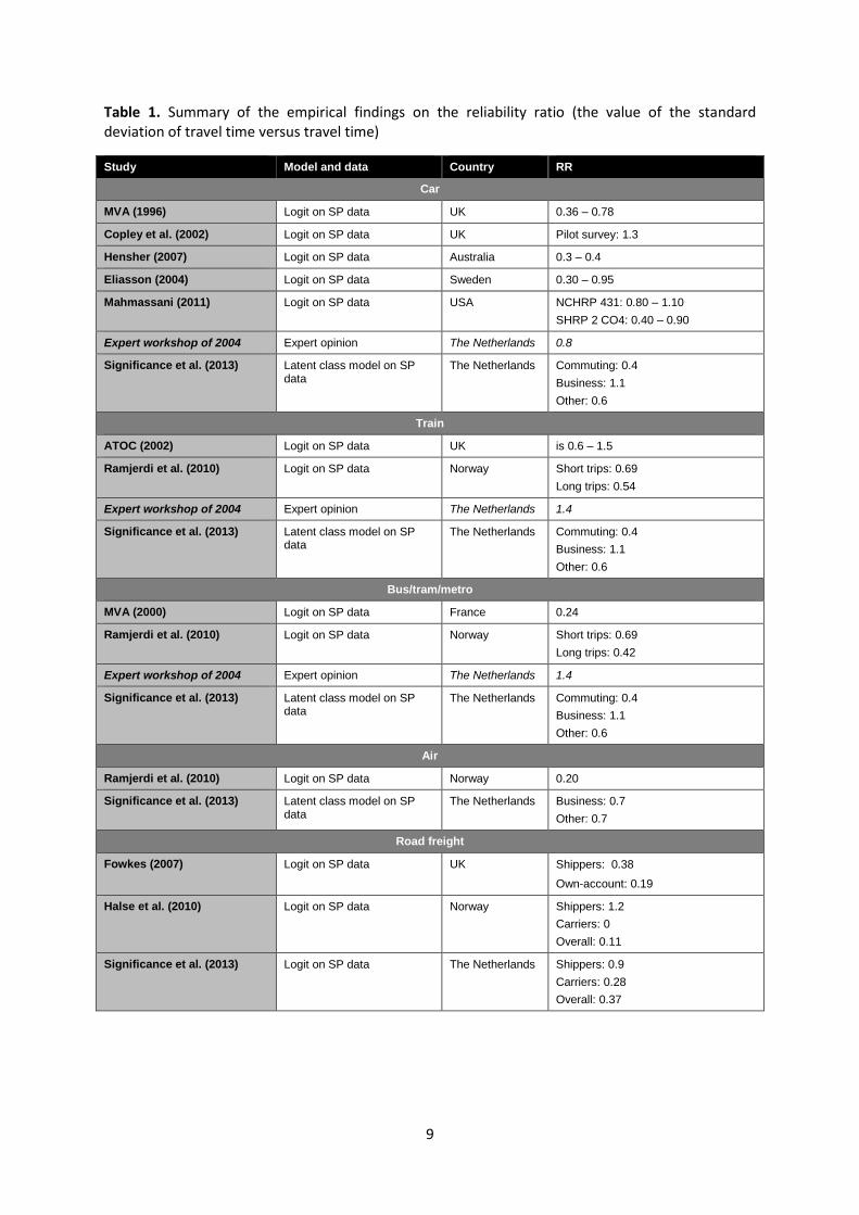
Given our choice for the standard deviation as best measure for reliability (at least in the short to medium run), the relevant P-side outcome is the monetary value of the standard deviation of journey time. This is often expressed in the form of the reliability ratio (RR): the value of reliability (measured as the standard deviation), VOR, divided by the value of time, VOT. Table 1 (adapted from

0

1

2

3

4

5

6

7

8

9

10

standarddeviation

variance bufferindex

punctuality scheduledelay

freq

uen

cy

8

Significance et al., 2013; also see Kouwenhoven et al., 2014, and de Jong et al., 2014) summarises empirical outcomes for various countries on the RR in passenger and freight transport that all use the same metric. Of course there is no guarantee that estimates for the standard deviation of travel time and thus for the RR are spatially transferable, so the preferred approach is estimating models on local data. More information about the international expert workshop in The Netherlands in 2004 can be found in Hamer et al. (2005). For passenger transport we obtain RRs between 0.2 and 1.5, with some concentration just below 1. The freight transport RR values are in general lower: between 0.1 and 0.4, but please note that the VOTs (used in the denominator of the RR) are substantially higher for a truck than for a car.

4. Review of travel time reliability forecasting models In this section we look at the Q-side, i.e. we will review travel time reliability forecasting models proposed in different countries for road transport. Most of these models deal with both passenger and freight transport (cars and trucks), though many studies do not make an explicit distinction between the two. United Kingdom In the United Kingdom, the Department for Transport (DfT) organised a seminar in 2001 to set out the research agenda on reliability. It was agreed that the biggest knowledge gaps were on the supply side (how can reliability be explained from its influencing factors?) and most of the subsequent research has indeed been on this topic, particularly for road transport. Nevertheless, despite some progress, Bates (2010) concluded that priority should continue to be given to the supply side. Arup (2003) estimated a relation between travel time reliability and congestion, based on the observation that variability is likely to be greater as flows reach capacity. They use the so-called congestion index (CI) as a key explanatory variable of variability, where CI is defined as the ratio of the mean travel time to the free flow travel time for a journey (note: not for a link). This gives model-users a simple way of generating travel time variances from standard data that already exists on mean travel times. Reliability or variability of travel time is measured as the coefficient of variation (CV = ratio of standard deviation to mean). Relationships between CV and CI were estimated (using route data from London and Leeds) and reported in Arup (2003). It was noticed that there was a tendency for the journey CV to decline with journey length D. The ‘compromise equation’ using both the London and Leeds data was of the form (included in the latest WebTAG guidance, Unit 3.5.7):

285.0781.0148.0 DCICV [4]

The above Arup model focuses on day-to-day variability of travel time. Frith et al. (2004) developed a model for incidents (such as car accidents) using data for dual carriageways. This model, called INCA (building on an older model called INCIBEN), explains how queues are formed when an incident happens, and can calculate benefits of fewer incidents and of additional capacity and takes account of changes in reliability. Sirivadidurage et al. (2009) extended INCA to include day-to-day variability as well, and also to include other road interurban and rural road types than just the dual carriageways. The measure of reliability that is used for motorways (and other non-urban roads) is the standard deviation.

9

Table 1. Summary of the empirical findings on the reliability ratio (the value of the standard deviation of travel time versus travel time)

Study Model and data Country RR

Car

MVA (1996) Logit on SP data UK 0.36 – 0.78

Copley et al. (2002) Logit on SP data UK Pilot survey: 1.3

Hensher (2007) Logit on SP data Australia 0.3 – 0.4

Eliasson (2004) Logit on SP data Sweden 0.30 – 0.95

Mahmassani (2011) Logit on SP data USA NCHRP 431: 0.80 – 1.10

SHRP 2 CO4: 0.40 – 0.90

Expert workshop of 2004 Expert opinion The Netherlands 0.8

Significance et al. (2013) Latent class model on SP data

The Netherlands Commuting: 0.4

Business: 1.1

Other: 0.6

Train

ATOC (2002) Logit on SP data UK is 0.6 – 1.5

Ramjerdi et al. (2010) Logit on SP data Norway Short trips: 0.69

Long trips: 0.54




Business: 1.1

Other: 0.6

Bus/tram/metro

MVA (2000) Logit on SP data France 0.24

Ramjerdi et al. (2010) Logit on SP data Norway Short trips: 0.69

Long trips: 0.42




Business: 1.1

Other: 0.6

Air

Ramjerdi et al. (2010) Logit on SP data Norway 0.20


The Netherlands Business: 0.7

Other: 0.7

Road freight

Fowkes (2007) Logit on SP data UK Shippers: 0.38

Own-account: 0.19

Halse et al. (2010) Logit on SP data Norway Shippers: 1.2

Carriers: 0

Overall: 0.11

Significance et al. (2013) Logit on SP data The Netherlands Shippers: 0.9

Carriers: 0.28

Overall: 0.37

10

Australia and New Zealand

In Australia and New Zealand, the Australian Transport Council (2006) and the NZ Transport Agency (2010) adopt the standard deviation of travel times are a measure of travel time unreliability. Both countries use the same method to calculate standard deviations. Similar to the method proposed in the UK, it computes the standard deviation as a function of the level of congestion on a road. Instead of using a congestion index, the volume-capacity ratio is used to describe the level of congestion on a specific road section or intersection. The following equation is used for calculating the standard deviation on a link/intersection level:

1exp1

00

CVb

sss [5]

where 0s is the lowest (uncongested) value of the standard deviation, s is the maximum (congested) value, V/C denotes the volume-capacity ratio, and b is a parameter. These values are different for different road types and intersection section types. For example, for a motorway, 0s 0.083, s 0.90, and b = -52, for an urban arterial road 0s 0.117, s 0.89, and b = -28, for a signalised intersection 0s 0.120, s 1.25, and b = -32, while for an unsignalised intersection

0s 0.017, s 1.20, and b = -22. In order to compute the route standard deviations, the square of all standard deviations is taken (creating variances), them summed along each route, and then a square root is taken. This way of obtaining the route standard deviation clearly ignores possible correlations between roads and intersections.

Wang (2014) contains a description of the road travel time reliability model for New South Wales (Australia). It explains the buffer time (defined as the 95th percentile minus the median of the travel time distribution) as a function of day-to-day traffic variation and road incidents (including the likelihood of being impacted by an incident and incident delay). This equation can be applied to data from a traffic flow model in combination with crash statistics. In project appraisal, the resulting predicted buffer time is given the same weight per minute as travel time.

The Netherlands

In The Netherlands, Besseling et al. (2004) try to develop a practical and provisional way to include variability in CBA and recommend, based on a literature research, multiplying the travel time benefits by 1.25 to include variability.

Meeuwissen et al. (2004) developed the model SMARA, which adopts a Monte Carlo simulation approach in order to create travel time distributions. In each simulation run, it takes a specific instance from the supply and demand distributions, and then computes a static user equilibrium assignment assuming vertical queues. Since the static assignment procedure does not consider horizontal (physical) queues as a (quasi) dynamic model would, the generated travel time distributions are only a rough approximation.

Efforts to include travel time variability in the Dutch National Model (LMS) for transport and the related New Regional Models (NRM) are reported in Kouwenhoven et al. (2005). The objective of this study was to develop a tool to predict future travel time reliability of networks, using exogenous variables that are available in the model (traffic intensity, speed, route length, speed limit). The study only deals with road traffic (though the model system is multimodal). Induction loop detectors provided speeds and traffic intensity measurements on the Dutch road network (in this case only highways). In the data set, the speeds and intensities are averaged over 15-minute (day-to-day) periods in the morning and evening peak, 212 routes with lengths between 2 and 120 km were identified on this network. Four reliability indicators were defined: (i) probability that a trip is ‘on time’ , (ii) probability that a journey is ‘not too long’, (iii) 10th percentile of the speed distribution

11

(T10), and (iv) 90th percentile of the speed distribution (T90). The best explanatory variable for probability ‘on time’ and ‘not too long’ turned out to be speed measured as route length divided by mean journey time, with a correction for the speed limit. The two percentile measures also depend on mean travel time, mean speed limit and journey length, such that improving journey times will also improve reliability. The impact of accidents (normal and severe), road works and rainfall were included in the regressions as factors that shift the speed curve away from the speed under perfect conditions. Also there is a conversion to reliability measured as the standard deviation, which is then used together with provisional values of reliability from Hamer et al. (2005) (also see de Jong et al., 2009) to calculate the unreliability costs.

Van Lint et al. (2007) state that travel time reliability indicators are mostly related to properties of the day-to-day travel time distribution on for example a freeway corridor. They study a particular time-of-day (and day-of-week) for a longer time, such as a year. This distribution is wide and heavily skewed; it has a long right tail. These very long travel times (much longer than expected) impose the highest costs for society. From this they conclude that most of the currently used unreliability measures (variance, standard deviation) should be used and interpreted with some reservations, since they do not explicitly account for the skewness, and are sensitive to outliers. They propose an unreliability indicator that includes both a measure of the width of the travel time distribution ((T90-T10)/T50) and of its skewness ((T90-T50)/(T50-T10)), where T denotes percentiles.

Tu (2009) develops a function where travel time unreliability on a motorway section is explained by the traffic inflow to that section. Unreliability is measured as the difference between the 90th and the 10th percentile of the travel distribution (at a given traffic inflow). He defines unreliability to include both travel time variability as well as travel time instability. If the traffic is below a critical transition inflow, travel time will be certain (no variability) and stable. Between this level and the critical capacity inflow, travel time will be uncertain and unstable. Above the critical capacity inflow level (that is in a situation close to capacity where a traffic breakdown can occur any time), travel times will be more certain but the traffic flow unstable (it is very likely that a few minutes later congestion will set in with ensuing smaller flows and longer travel times). Tu’s equations for unreliability distinguish between these regimes. An approximate travel time unreliability function is given by:

TTUR(qin) = TTUR0 (1+ (qin/ttr)) [6]

where TTUR(qin) is the travel time unreliability for a given inflow qin, TTUR0 is the free flow travel

time unreliability, ttr is the critical travel time unreliability inflow, and and are parameters. In a separate analysis, Tu relates travel time reliability to road geometry, speed limits, accidents and weather. The reliability equations were calibrated to speed measurement data (at 10 minutes intervals) at various motorways in The Netherlands (converted to travel times using a trajectory method). Li et al. (2009) proposes a dynamic network model with route and departure time choice with fluctuating network capacities. Travel time reliability is assumed to influence these travel choices via a generalized cost function, consisting of the mean travel time, the standard deviation of travel time, and early and late schedule delay components. A Monte Carlo simulation approach is adopted in order to determine the network travel time reliability is using many draws from the distribution of network capacities. An important finding is, that the travel time reliability (in terms of standard deviation) does not exhibit an increasing relationship with the mean travel time. Therefore, they conclude that a simple (often linear) relationship between the standard deviation and the mean travel time is not valid.

Hellinga (2011) analysed the relationship between the standard deviation of route travel times, versus the annual average travel time. He used data loop detector data from a single motorway and calculated travel times for 255 non-holiday workdays in 2009. Taking out extreme travel time data that occur as a result of an incident, severe weather, temporary road closures and other non-

12

recurrent conditions, an almost linear relationship (with R2 of 0.89) was found between the average travel time (TT) and the standard deviation ( ):

TT9589.0091.11 [7]

Peer et al. (2012) try to provide simple prediction rules for variability for road traffic. They are only looking at variations in travel times that are not expected by drivers. They use two different concepts of travel time variability, depending on whether the driver has only rough or fine information on expected travel times. In the first (rough information) they assume that for a given road link expected travel time is constant across all working days. In the second (fine information), expected travel times reflect day-specific factors such as the weather or the day of the week, season. In both cases they use the standard deviation of travel time as the variability measure. Speeds from loop detectors from 145 different highway segments are used to perform separate regressions for each segment and each 15-minute period. They find both for the rough and the fine information case a positive relation between variability and mean delay (the difference between observed and free flow travel time), but the relation is not linear: the first derivative of variability with respect to mean delay is decreasing in delay. For longer delays, the relationship is close to linear.

Kouwenhoven (2014) contains model estimations on detection loop data (for motorways) and camera data (for other roads). This work is meant as the successor of Kouwenhoven et al. (2005) and the estimated models were implemented as a new post-processing module of the Dutch national model LMS and regional models NRM. The data for estimation refer to 251 working days in 2012 for 250 motorway routes (between 2 and 225 km long) and 40 non-motorway routes (between 1 and 11 km) per 15-minute period. Many different specifications were tried to explain the standard deviation of a route and time period combination, using the literature that is also reviewed in this paper. The best results are obtained when using a combination of a linear and logarithmic function for the mean delay, and an added linear term for the route length. Higher order terms were not found significant.

σ = a + b.MD + c.ln(MD+1) + d.D [8]

MD is the mean delay (the difference between observed and free flow travel time), D is route length, and a, b, c and d are coefficients to be estimated.

Sweden

In Sweden, Eliasson (2006) uses two weeks of continuous travel time measurements on 84 links on street and road in around central Stockholm. The data is split into 15-minute periods. The relative standard deviation is then calculated (this is the standard deviation of travel time divided by travel time) and explained in a regression analysis. The main explanatory variable is a measure of congestion: travel time divided by free flow travel time. Using a traffic model that can predict the amount of congestion, one can also calculate the changes in the amount of unreliability, for use in CBA. The SILVESTER model, as used in Kristoffersson and Engelson (2008) and Kristofferson (2011), is a dynamic mode, route, and departure time model including a reliability forecasting model (based on Eliasson, 2006). The departure time choice model contains terms for scheduling delays and for the standard deviation of the travel times. This model has been used to study the impacts of the Stockholm congestion charging and many alternative variants of the charging scheme. SILVESTER is one of very few operational transport models in the world where reliability affects the behaviour of travellers and where the reliability benefits do not come from a post-processing module.

13

Denmark

In Denmark, Fosgerau and Fukuda (2010) used speed and traffic flow measurement data on a road with four consecutive links with a total length of 11 km connecting to the city centre of Copenhagen. This data consists of minute by minute observations of travel time in the morning peak for over five months. They estimated models for the mean travel time and reliability measured as the interquartile range (75th-25th percentile), using non-parametric techniques. They found that the standardised travel distribution is far from a Normal distribution but close to a stable distribution. The latter distribution however does not give a good description of extreme delays, which are overestimated (fatter extreme right tails than observed). This could be remedied by truncating the stable distribution. They also found that the standardised travel times seem to be close to independent across links of the same route. This makes calculating the travel time distribution (or reliability) for the route on the basis of the results for the links considerably easier.

United States

In the United States, since 2005 the Transportation Research Board (TRB) has a research program SHRP2 (Strategic Highway Research Program) with four components: safety, renewal, reliability and capacity. The reliability component includes several projects to reduce and prevent non-recurrent congestion and develop a tool for identifying and evaluating the costs and effectiveness of design features (of highways) that can improve travel time reliability. Within SHRP 2, L04 studies the issue of incorporating reliability performance measures in operations and planning modelling tools. TRB SHRP2 describes congestion and reliability measures on more than 300 corridors in big metropolitan regions in the US. This report however focuses on hours and additional travel time, not on including reliability in the CBA. Within SHRP2, L03 studies analytical procedures for determining impacts of reliability mitigation strategies. In this project, models have been developed to estimate the standard deviation of (link or route) travel times as a function of the mean travel time. To be more precise, several researchers have shown an almost linear relationship between the standard deviation of route travel times and the normalized route travel time (which is the route travel time divided by the route distance). Mahmassani (2011) illustrated this on two networks (Washington DC and Irvine CA). Linear regression models were fitted on this data of the form

σ = a + b (T / D) [9]

where σ is the standard deviation of (T/D) on a route (OD) level, T is the route travel time, D is the travel distance, and a and b are parameters to be estimated. The fit of this model, as indicated by the R2, was 0.67. It was recognized that a distinction has to be made between recurrent (typical day) congestion, and non-recurrent congestion due to incidents, weather, and special events. Transportation models will typically only produce results for recurrent congestion, on which they are calibrated. Let the travel time index be defined by

TIi = Ti / Ti0 [10]

where TIi is the travel time index for day i for a certain route and departure time, Ti is the travel time, and Ti

0 is the free-flow travel time. Let TI denote the mean travel time index over all days. Then the following empirical relationship has been estimated, that converts the recurrent travel time index by the overall (recurrent plus non-recurrent) travel time index TIall:

TIall = 1.0274 TI1.2204 [11]

In other words, they determine the non-recurrent travel time delays as a supplement on the recurrent travel time delays. Then in the next step another empirical relationship is estimated, that expresses the relationship between the standard deviation σ on a route with the overall travel time index:

14

σ = 0.6182 (TIall -1) 0.5404 [12]

Gayah et al. (2013) try to explain the phenomenon that is sometimes observed in empirical data for a single bottleneck within a small urban network that the travel time variance is larger during congestion recovery than during the onset of congestion. They develop a theoretical model for day-to-day travel time variation that includes hysteresis loops and validated this model successfully on micro-simulation data for Orlando, Florida.

Germany

In Germany a study was carried out recently for the BMVDI to estimate establish a function explaining the travel time reliability on motorways (Geistefeldt et al., 2014). This study used a power-law function between the standard deviation and the mean delay:

σ = a (MD)b [13]

The estimation took place on simulated data, obtained using a macroscopic traffic simulation model (that has been validated on empirical data on traffic flows and travel times that were available for a specific part of Germany (Hessen)). All previously mentioned relations can be used to obtain the impact of a project or policy on reliability, by first taking its impact on travel time or link flow and then using the estimated relation between the standard deviation of travel time and this variable. However, some policy measures have very different impacts on travel time and travel time reliability. The introduction of a maximum speed for instance is likely to increase travel times, but may reduce variability by making speeds more homogeneous. Several projects have therefore expressed impacts on reliability without making use of travel time as intermediate variable, often by distinguishing ‚‘typical‘ sorts of policy measures for which the impact can be looked up in a table. Examples of such studies are Mott MacDonald (2009) for UK motorways and Palsdottir (2011) for policy measures on motorways roads in The Netherlands. The reliability component of SHRP2 in the US also includes a project to develop a tool for identifying and evaluating the costs and effectiveness of design features (of highways) that can improve travel time reliability.

5. Recommendations for the medium, medium to long and long term Based on the literature review and the results from the expert interviews and the meeting, we can say there is some kind of agreement on the methodology to use in order to assess unreliability in cost-benefit analyses, although not all researchers and experts have identical views. It is clear that it is a complex topic and that more research is needed to provide answers to several questions. Nevertheless, we feel confident that the recommendations made in this section will be in agreement with the opinion of the majority of the experts. We think these recommendations are valid for all countries and regions that carry out CBAs for project appraisal using (aggregate or disaggregate) transport models that can produce route travel times, but do not contain a departure time choice (scheduling) model.

5.1 Three methods: a simple feasible approach, an intermediate approach, an ideal approach

Below, we describe three different methods. The first method is a simple approach that can be implemented within 2 to 3 years and does not require any adjustments with respect to the transport model and has a short computation time. The second method is a more advanced approach that can be implemented within 3 to 5 years, but requires some changes to the transport model and has a longer computation time. The third method can to some extent be referred to as the ideal model

15

that could be implemented in 10+ years, but requires significant changes to the transport model, and due to necessary simulations requires very long computation times.

Method 2 builds on method 1, and could be developed as an extension after first having carried out method 1. Method 3 is a different approach in several ways: if method 1 and 2 would be carried out first, some elements from these alternatives could be re-used, but several things would have to be developed again –but differently– from the start.

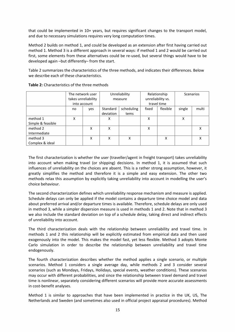
Table 2 summarizes the characteristics of the three methods, and indicates their differences. Below we describe each of these characteristics.

Table 2: Characteristics of the three methods

The network user takes unreliability

into account

Unreliability measure

Relationship unreliability vs.

travel time

Scenarios

no yes Standard deviation

scheduling tems

fixed flexible

single multi

method 1 Simple & feasible

X X X X

method 2 Intermediate

X X X X

method 3 Complex & ideal

X X X X X

The first characterization is whether the user (traveller/agent in freight transport) takes unreliability into account when making travel (or shipping) decisions. In method 1, it is assumed that such influences of unreliability on the choices are absent. This is a rather strong assumption, however, it greatly simplifies the method and therefore it is a simple and easy extension. The other two methods relax this assumption by explicitly taking unreliability into account in modelling the user’s choice behaviour.

The second characterization defines which unreliability response mechanism and measure is applied. Schedule delays can only be applied if the model contains a departure time choice model and data about preferred arrival and/or departure times is available. Therefore, schedule delays are only used in method 3, while a simpler dispersion measure is used in methods 1 and 2. Note that in method 3 we also include the standard deviation on top of a schedule delay, taking direct and indirect effects of unreliability into account.

The third characterization deals with the relationship between unreliability and travel time. In methods 1 and 2 this relationship will be explicitly estimated from empirical data and then used exogenously into the model. This makes the model fast, yet less flexible. Method 3 adopts Monte Carlo simulation in order to describe the relationship between unreliability and travel time endogenously.

The fourth characterization describes whether the method applies a single scenario, or multiple scenarios. Method 1 considers a single average day, while methods 2 and 3 consider several scenarios (such as Mondays, Fridays, Holidays, special events, weather conditions). These scenarios may occur with different probabilities, and since the relationship between travel demand and travel time is nonlinear, separately considering different scenarios will provide more accurate assessments in cost-benefit analyses.

Method 1 is similar to approaches that have been implemented in practice in the UK, US, The Netherlands and Sweden (and sometimes also used in official project appraisal procedures). Method

16

2 resembles some of the current plans in these countries, but there are hardly any practical examples yet (an exception is the SILVESTER model for Stockholm, that also includes features of method 3). Alternative 3 clearly goes beyond today’s best practice, and in some ways even beyond the state-of-the art: further research will be needed to make this possible.

5.2 Method 1: Least comprehensive – most feasible

In this method, the transport models are not altered to include reliability. To include reliability in the CBA, a new separate reliability module will be developed, that uses outputs of the transport model to predict future values of reliability. This is a so-called post-processing module; its outputs will not feed back to the transport model: there is only a one-way-communication between the transport model and the new reliability module. A disadvantage of this is that the transport demand in the transport model and the reliability model will not be fully consistent: in reality, agents (travellers and other decision-makers in freight transport) will react to changes in reliability, and the demand that the transport models produce will not be in equilibrium with the predicted reliability levels. In this method, we assume that agents will not react to changes in reliability, and we calculate the consequences of reliability changes for society at unchanged behaviour. Such a post-processing procedure is also applied in Australia and New Zealand, although we propose to adopt a different computation method.

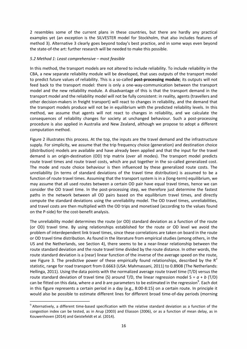
Figure 2 illustrates this process. At the top, the inputs are the travel demand and the infrastructure supply. For simplicity, we assume that the trip frequency choice (generation) and destination choice (distribution) models are available and have already been applied and that the input for the travel demand is an origin-destination (OD) trip matrix (over all modes). The transport model predicts route travel times and route travel costs, which are put together in the so-called generalized cost. The mode and route choice behaviour is then influenced by these generalized route costs. The unreliability (in terms of standard deviations of the travel time distribution) is assumed to be a function of route travel times. Assuming that the transport system is in a (long-term) equilibrium, we may assume that all used routes between a certain OD pair have equal travel times, hence we can consider the OD travel time. In the post-processing step, we therefore just determine the fastest paths in the network between all OD pairs based on the equilibrium travel times, and directly compute the standard deviations using the unreliability model. The OD travel times, unreliabilities, and travel costs are then multiplied with the OD trips and monetised (according to the values found on the P-side) for the cost-benefit analysis.

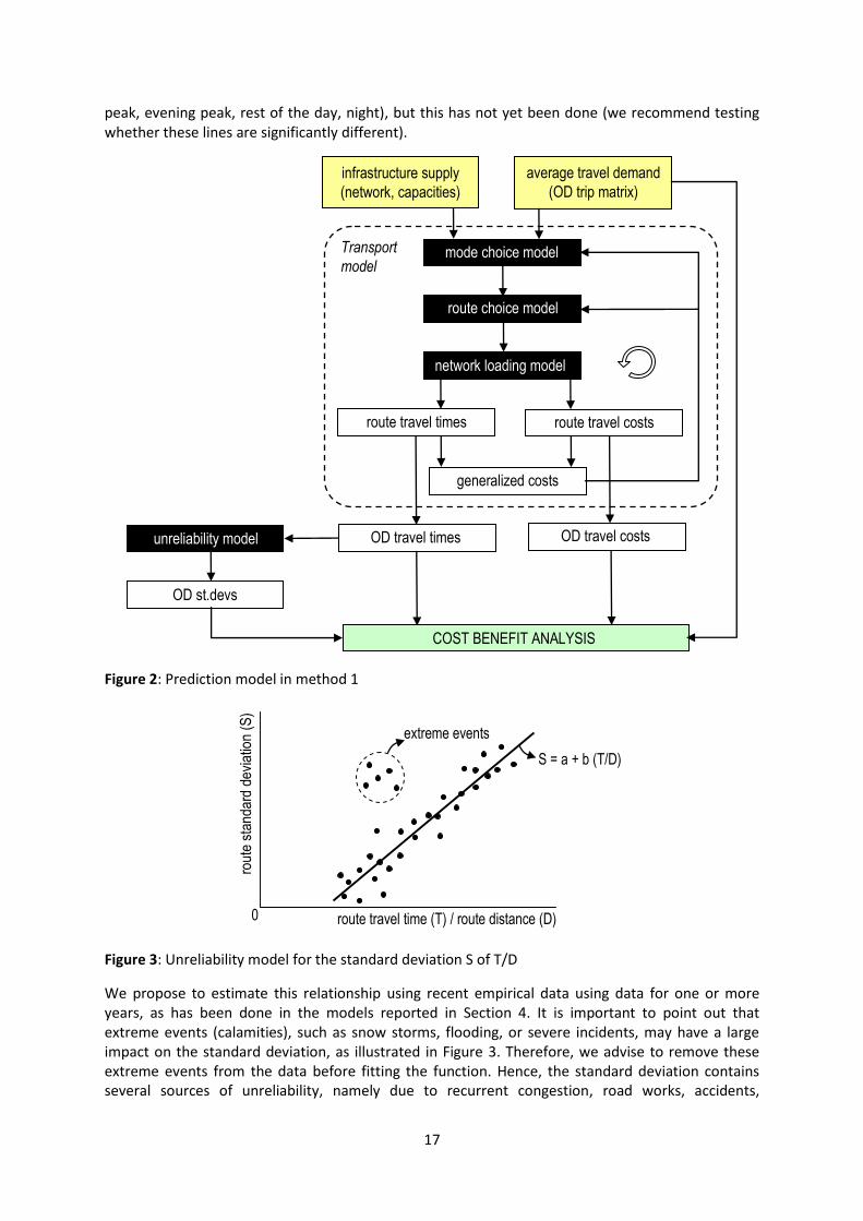
The unreliability model determines the route (or OD) standard deviation as a function of the route (or OD) travel time. By using relationships established for the route or OD level we avoid the problem of interdependent link travel times, since these correlations are taken on board in the route or OD travel time distribution. As found in the literature from empirical studies (among others, in the US and the Netherlands, see Section 4), there seems to be a near-linear relationship between the route standard deviation and the route travel time divided by the route distance. In other words, the route standard deviation is a (near) linear function of the inverse of the average speed on the route, see Figure 3. The predictive power of these empirically found relationships, described by the R2 statistic, range for road transport from 0.6663 (USA: Mahmassani, 2011) to 0.8908 (The Netherlands: Hellinga, 2011). Using the data points with the normalized average route travel time (T/D) versus the route standard deviation of travel time (S) around T/D, the linear regression model S = a + b (T/D) can be fitted on this data, where a and b are parameters to be estimated in the regression9. Each dot in this figure represents a certain period in a day (e.g., 8:00-8:15) on a certain route. In principle it would also be possible to estimate different lines for different broad time-of-day periods (morning

9 Alternatively, a different time-based specification with the relative standard deviation as a function of the

congestion index can be tested, as in Arup (2003) and Eliasson (2006), or as a function of mean delay, as in Kouwenhoven (2014) and Geistefeldt et al. (2014).

17

peak, evening peak, rest of the day, night), but this has not yet been done (we recommend testing whether these lines are significantly different).

Figure 2: Prediction model in method 1

Figure 3: Unreliability model for the standard deviation S of T/D

We propose to estimate this relationship using recent empirical data using data for one or more years, as has been done in the models reported in Section 4. It is important to point out that extreme events (calamities), such as snow storms, flooding, or severe incidents, may have a large impact on the standard deviation, as illustrated in Figure 3. Therefore, we advise to remove these extreme events from the data before fitting the function. Hence, the standard deviation contains several sources of unreliability, namely due to recurrent congestion, road works, accidents,

mode choice model

route choice model

network loading model

route travel times route travel costs

average travel demand

(OD trip matrix)

infrastructure supply

(network, capacities)

generalized costs

Transport

model

OD st.devs

mnreliability model

COST BENEFIT ANALYSIS

unreliability model OD travel times OD travel costs

route travel time (T) / route distance (D)

rou

te s

tan

da

rd d

evi

atio

n (

S)

extreme events

S = a + b (T/D)

0

18

unexpected weather conditions, and the random component in day-to-day variation in travel times. This will provide an approximation of the unreliability of the system, without considering robustness (sensitivity of the network to extreme events).

An alternative to the above approach would be to use an unreliability model as a function of the inflow. However, there are several drawbacks to this approach, as denoted by Hellinga (2011). First of all, the model needs to be calibrated for each route, it is unknown whether the parameters can be transferred to other routes. Secondly, it is unclear how the model will behave with different on- and off-ramps. Thirdly, policies or measures that do not influence the inflow will have no impact on the estimated travel time reliability. Therefore, we do not recommend this approach. Explaining reliability on the basis of travel time has some practical consequences. First this makes it difficult to simulate the impact of policies (such as changing the maximum speed) that have a very different effect on mean travel time and on reliability. Such policy situations can be seen as moving to a fundamentally different line, which however would be very difficult to estimate because data is lacking. For policies such as supplying additional road capacity, the estimated line can be used as it is, with mean travel time and the standard deviation moving in the same direction. Also one might argue that if the standard deviation would be proportional to travel time, than one could include reliability benefits in the CBA simply by a multiplicative factor times the travel time benefits. This argument does not hold however, because in the reliability model every travel time should be divided by its corresponding distance (e.g. at the OD level). So there still is a case for calculating the size of the reliability benefits for each route or OD.

5.3 Method 2: Intermediate

This alternative includes everything that was also in the first alternative, but extended with scenarios and a feedback loop in the prediction model that takes reliability into account in the agents’ behaviour. In method 1, the reactions of the travellers and the decision-makers in freight transport to changes in reliability are not taken into account. As in method 1, we propose to use the standard deviation as the measure that defines unreliability.

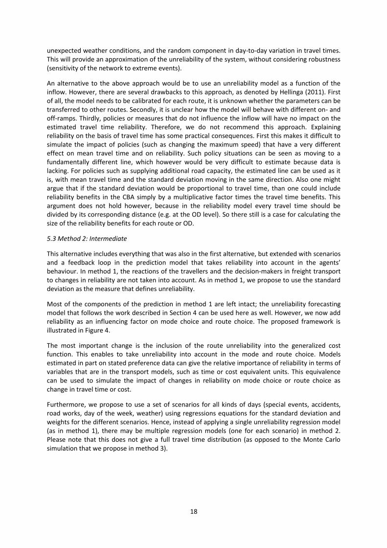
Most of the components of the prediction in method 1 are left intact; the unreliability forecasting model that follows the work described in Section 4 can be used here as well. However, we now add reliability as an influencing factor on mode choice and route choice. The proposed framework is illustrated in Figure 4.

The most important change is the inclusion of the route unreliability into the generalized cost function. This enables to take unreliability into account in the mode and route choice. Models estimated in part on stated preference data can give the relative importance of reliability in terms of variables that are in the transport models, such as time or cost equivalent units. This equivalence can be used to simulate the impact of changes in reliability on mode choice or route choice as change in travel time or cost.

Furthermore, we propose to use a set of scenarios for all kinds of days (special events, accidents, road works, day of the week, weather) using regressions equations for the standard deviation and weights for the different scenarios. Hence, instead of applying a single unreliability regression model (as in method 1), there may be multiple regression models (one for each scenario) in method 2. Please note that this does not give a full travel time distribution (as opposed to the Monte Carlo simulation that we propose in method 3).

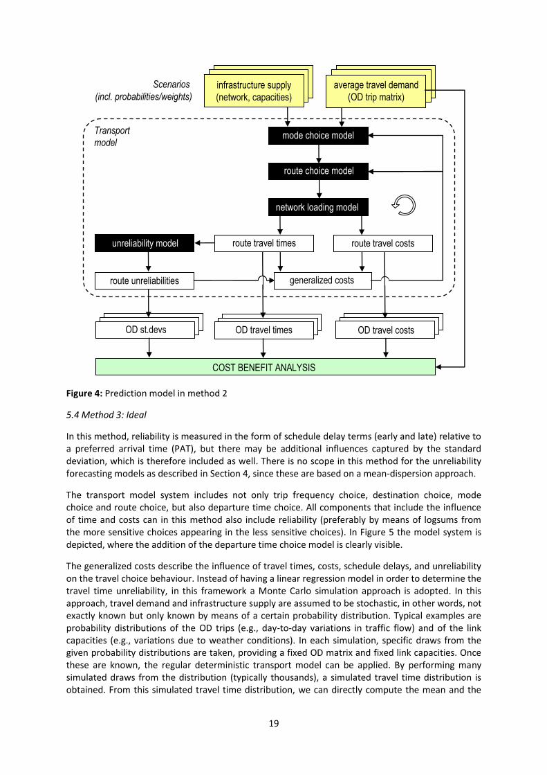
19


5.4 Method 3: Ideal

In this method, reliability is measured in the form of schedule delay terms (early and late) relative to a preferred arrival time (PAT), but there may be additional influences captured by the standard deviation, which is therefore included as well. There is no scope in this method for the unreliability forecasting models as described in Section 4, since these are based on a mean-dispersion approach.

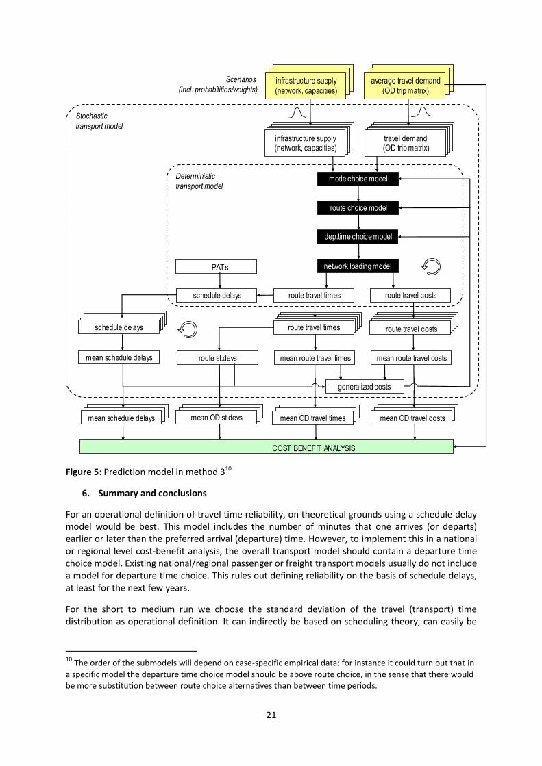
The transport model system includes not only trip frequency choice, destination choice, mode choice and route choice, but also departure time choice. All components that include the influence of time and costs can in this method also include reliability (preferably by means of logsums from the more sensitive choices appearing in the less sensitive choices). In Figure 5 the model system is depicted, where the addition of the departure time choice model is clearly visible.

The generalized costs describe the influence of travel times, costs, schedule delays, and unreliability on the travel choice behaviour. Instead of having a linear regression model in order to determine the travel time unreliability, in this framework a Monte Carlo simulation approach is adopted. In this approach, travel demand and infrastructure supply are assumed to be stochastic, in other words, not exactly known but only known by means of a certain probability distribution. Typical examples are probability distributions of the OD trips (e.g., day-to-day variations in traffic flow) and of the link capacities (e.g., variations due to weather conditions). In each simulation, specific draws from the given probability distributions are taken, providing a fixed OD matrix and fixed link capacities. Once these are known, the regular deterministic transport model can be applied. By performing many simulated draws from the distribution (typically thousands), a simulated travel time distribution is obtained. From this simulated travel time distribution, we can directly compute the mean and the

mode choice model

route choice model




(OD trip matrix)



generalized costs

Transport

model

route unreliabilities

mnreliability model


unreliability model

OD travel times OD travel costsOD st.devs

Scenarios

(incl. probabilities/weights)

20

standard deviation, but also the arrival time distribution. We can also compute a schedule delay early term or a schedule delay late term for each draw. Hence, instead of including a fixed relationship between the mean travel time and the standard deviation of travel time (from empirical data), the whole distribution is simulated. This provides a large degree of flexibility in which the effect of any possible scenario can be simulated, and is not restricted to a linear relationship. In method 1 and 2, we considered the unreliability to be an increasing function of the travel time. This may not always be the case (example: decreasing the speed limit from 120 km/h to 80 km/h will increase the travel time, but may decrease the unreliability because of speed harmonisation). Such a flexible relationship as in method 3 should therefore be preferred. On the other hand, such a simulation approach is very time consuming, as for each iteration in the transport model, a Monte Carlo simulation needs to be conducted. Even with current computational power and parallelization techniques, such an approach is not (yet) feasible on practical networks. Furthermore, when relying on model predicted travel times, scheduling terms and standard deviations instead of empirical travel times and standard deviations, it is essential that the model is able to predict these values with a sufficient accuracy. Traditional static network loading techniques are not adequate, hence one has to rely on quasi-dynamic or dynamic network loading procedures in which the location of the queues and the length of the queues are explained well. This adds to the computational complexity of the whole system.

Under strict assumptions in traditional static traffic assignment models, it may be possible to avoid Monte Carlo simulations and express travel time unreliability analytically. For example, Uchida (2014) shows that travel time variances can be approximated analytically by assuming independence between link travel times or assuming fixed exogenous correlation coefficients between link flows. However, both assumptions are unrealistic and limit the applicability. As in method 2, scenarios are still used in this method, in which different days of the week or holiday periods can have different travel demand and infrastructure supply probability distributions.

This method requires a stated/revealed preference survey that goes beyond that in method 1 and 2 in that it will also include departure and arrival time as attributes or as choice alternatives (see for instance the description in Arellana et al., 2013). Also the survey should ask for PATs for the observed trip. It would be best to try to include both schedule delay terms and the standard deviation of travel time as explanatory variables for the choices made, because there may be scope for the simultaneous presence of both.

21


6. Summary and conclusions

For an operational definition of travel time reliability, on theoretical grounds using a schedule delay model would be best. This model includes the number of minutes that one arrives (or departs) earlier or later than the preferred arrival (departure) time. However, to implement this in a national or regional level cost-benefit analysis, the overall transport model should contain a departure time choice model. Existing national/regional passenger or freight transport models usually do not include a model for departure time choice. This rules out defining reliability on the basis of schedule delays, at least for the next few years.

For the short to medium run we choose the standard deviation of the travel (transport) time distribution as operational definition. It can indirectly be based on scheduling theory, can easily be

10 The order of the submodels will depend on case-specific empirical data; for instance it could turn out that in

a specific model the departure time choice model should be above route choice, in the sense that there would be more substitution between route choice alternatives than between time periods.

mean schedule delays mean OD travel times mean OD travel costsmean OD st.devs

mode choice model

route choice model




(OD trip matrix)



generalized costs


route travel times route travel costsschedule delays

Stochastic

transport model

travel demand (OD trip matrix)

infrastructure supply(network, capacities)

dep.time choice model

schedule delays

PATs

mean route travel times mean route travel costsroute st.devsmean schedule delays

Deterministic

transport model

Scenarios

(incl. probabilities/weights)

22

calculated from available data and often provides a good explanation of choices made in SP experiments. It also was the measure that was recommended by most experts that we interviewed.

The existing variation in travel time is caused by demand variation over times-of-day and between days of the week and seasons, the weather, road works and other works, accidents and extreme events and calamities. We recommend excluding the latter two influences from the operationalisation of reliability, but including all variation that travellers and freight operators (can) know in the expected time benefit and the remaining unknown variation in the reliability benefits.

To include travel time reliability (or transport time reliability for freight transport) in the cost-benefit analysis, three types of information are needed:

Monetary values to convert reliability benefits into money units;

A model that predicts how the infrastructure projects that need to be evaluated will influence reliability;

A model that predicts the reactions of travellers and decision-makers in freight transport (or of more aggregate transport demand) to changes in reliability.

Most studies on travel time reliability in the international literature deal with the first issue, the P-side of reliability. Some countries now have official values of reliability available, also for reliability defined as the standard deviation of travel time. The first and second issue (together the ‘Q-side’ of reliability) have been studied to a lesser degree. Practically all of these studies on the Q-side have dealt with road transport, trying to explain the standard deviation of travel time on motorways from travel time, inverse speed, congestion or traffic flow. The data used for this were automatic induction loop speed and flow measurements or GPS data. For public transport, it is common practice in some countries to monitor the deviations from the timetable as a measure reliability, but there are very few studies on modelling the Q-side of reliability in public transport, including van Oort (2011) on urban public transport and Hollander (2006), Hollander and Liu (2008) and Hollander and Buckmaster (2010) on the reliability of buses. To our best knowledge, regression relationships as have been estimated for road transport have not been reported for rail transport yet. For rail, deviations from the timetable are often not so much caused by congestion-related factors (crowding), but by technical or logistical problems at the operational vehicle or infrastructure level. Nevertheless, it should be possible to estimate equations explaining the standard deviation of travel time from the explanatory variables, which may include technical disturbances (trains, tracks) and excess demand, but also policy measures (such as electrification) directly.

For road transport (including passenger cars, vans, trucks and buses), we distinguish 3 methods to deal with the Q-side of reliability:

Method 1, which is relatively easy to implement in the next two-three years;

Method 2, which would take more effort and about three-five years to implement;

Method 3, which contains the ideal long-run solution. In method 1, the transport model will not be changed, but its outputs in terms of road travel times between origins and destination will be used to calculate the standard deviation of travel time for the reference case (without the infrastructure project) and the policy case (with the project). This will be done using a regression for road transport at the route level that needs to be estimated on data on travel times on motorways and other main roads. This unreliability model will then be a post-processing module, that is positioned after the transport model and that will provide reliability benefits for use in the cost-benefit analysis.

In method 2, reliability will also be included in the mode choice and route choice components of the transport models. In method 3, Monte Carlo simulation will give variations in demand and capacity

23

that lead to differences in travel time, from which one can calculate the average and standard deviation, for use in the cost-benefit analysis.

As stated in the introduction, including travel time reliability benefits is important in economic appraisal and policy making. Methods 1 and 2 outlined above present short term and medium term solutions to include such user benefits in cost-benefit analysis, which governments can implement within five years into existing transport models.

Acknowledgments This review was part of a project financed by the German Federal Ministry of Transport, Building and Urban Development (Bundesministerium für Verkehr, Bau und Stadtentwicklung, BMVBS, now BMVDI). We would like to thank the BMVBS and the experts we interviewed for their contributions to this project. The views and recommendations presented in this paper reflect opinions of the authors of this paper, and not necessarily the opinion of BMVBS/BMVDI. The useful comments and suggestions of two anonymous referees are gratefully acknowledged. References Arellana, J., Daly, A., Hess, S., Ortúzar, J. de D. and Rizzi, L. (2012) Development of Surveys for Study of Departure Time Choice. Transportation Research Record: Journal of the Transportation Research Board 2303: pp. 9-18.

Arellana, J., Ortúzar, J. de D. and Rizzi, L. (2013) Survey data to model time-of-day choice: methodology and findings. in Transport Survey Methods: Best Practice for Decision Making, eds J. Zmud., M. Lee-Gosselin, M. Munizaga and J.A. Carrasco, pp. 479-505. Emerald, Bingley (UK).

Arup (2003) Frameworks for Modelling the Variability of Journey Times on the Highway Network. Arup, London.

Association of Train Operating Companies (ATOC) (2002) Passenger Demand Forecasting Handbook. ATOC, London.

Australian Transport Council (2006) National guidelines for transport system management in Australia, Volume 5 (Background material). Canberra, Australia.

Bates, J. (2010) Stock-take of Travel Time Variability, produced for ITEA Division, UK Department for Transport. Abingdon, November 2010.

Bates, J., Polak J., Jones, P. and Cook, A. (2001) The valuation of reliability for personal travel. Transportation Research E (Logistics and Transportation Review), 37-2/3, pp. 191-229.

Besseling, P., de Groot, W. and Verrips, A. (2004) Economische toets op de Nota Mobiliteit, CPB document 65, CPB, The Hague.

Börjesson, M., Eliasson, J. and Franklin, J.P. (2012) Valuations of travel time variability in scheduling versus

mean–variance models. Transportation Research B, 46 (7), pp. 855-873.

Carrion, C. and D. Levinson (2012) Value of travel time reliability: A review of current evidence. Transportation Research A, 46, pp. 720-741.

Copley, G., Murphy, P. and Pearce, D. (2002) Understanding and valuing journey time variability. European Transport Conference – 2002, Cambridge.

Eliasson, J. (2004) Car drivers’ valuations of travel time variability, unexpected delays and queue driving. European Transport Conference – 2004, Strasbourg.

Eliasson, J. (2006) Forecasting travel time variability. European Transport Conference – 2006, Strasbourg.

Fosgerau, M. and Engelson, L. (2011) The value of travel time variance. Transportation Research B, 45(1), pp.

24

1-8.

Fosgerau, M. and Fukuda D. (2010) Valuing travel time variability: characteristics of the travel time distribution on an urban road. working paper, DTU Denmark.

Fosgerau, M. and Karlström, A. (2010) The value of reliability. Transportation Research B, 44(1), pp. 38-49.

Fowkes, T. (2007) The design and interpretation of freight stated preference experiments seeking to elicit behavioural valuations of journey attributes. Transportation Research B, 41, pp. 966-980.

Frith, B.A., Fearon, J., Sutch, T.E. and Lunt, G. (2004) Updating and validating parameters for incident appraisal model INCA. TRL Published Report PPR 020.

Gayah, V.V., Dixit, V.V. and Guler, S.I. 92013) Relationship between mean and day-to-day variation in travel time in urban networks. EURO Journal of Transportation and Logistics, DOI 10.1007/s13676-013-0032-2.

Geistefeldt, J., Hohmann, S. and Wu, N. (2014) Ermittlung des Zusammenhangs von Infrastruktur und Zuverlässigkeit des Verkehrsablaufs für den Verkehrsträger Straße – Schlussbericht für Bundesministerium für Verkehr und digitale Infrastruktur. Ruhr Universität Bochum.

Halse, A., Samstad, H. Killi, M. Flügel, S. and Ramjerdi, F (2010) Valuation of freight transport time and reliability (in Norwegian). TØI report 1083/2010, Oslo.

Hamer, R., De Jong, G.C. and Kroes, E.P. (2005) The value of reliability in Transport – Provisional values for the Netherlands based on expert opinion. RAND Technical Report Series, TR-240-AVV, Netherlands.

Hellinga, B. (2011) Defining, Measuring, and Modelling Transportation Network Reliability. Final report, Delft University of Technology, the Netherlands.

Hensher, D.A. (2007) Valuation of Travel Time Savings, prepared for the Handbook in Transport Economics, edited by André de Palma, Robin Lindsey, Emile Quinet, Roger Vickerman (Edward Elgar Publisher).

Hollander, Y. (2006) Direct versus indirect models for the effects of unreliability. Transportation Research A, 40(9), pp. 699-711.

Hollander, Y. and Buckmaster, M. (2010) The reliability component in project evaluation. Paper presented at the 89th Annual Meeting of the Transportation Research Board, January 2010, Washington D.C.

Hollander, Y. and Liu, R. (2008) Estimation of the Distribution of Travel Times by Repeated Simulation. Transportation Research C, Vol. 16, No. 2, pp. 212-231.

Jong, G.C. de, Kouwenhoven, M.L.A., Kroes, E.P., Rietveld, P. and Warffemius P.(2009) Preliminary monetary values for the reliability of travel times in freight transport. European Journal of Transport and Infrastructure Research, Issue 9(2), pp. 83-99.

Jong, G.C. de, Kouwenhoven, M., Bates, J.J., Koster, P., Verhoef, E.T., Tavasszy, L. and Warffemius, P. (2014) New SP-values of time and reliability for freight transport in the Netherlands. Transportation Research E, 64, pp. 71-87.

Kouwenhoven, M., Jong, G.C. de, Koster, P., Berg, V.A.C. van den, Verhoef, E.T., Bates, J.J., and Warffemius, P. (2014) New values of time and reliability in passenger transport in The Netherlands. Research in Transportation Economics, 47, pp. 37-49.

Kouwenhoven, M.L.A., Schoemakers, A., Grol, R. Van, Kroes, E.P. (2005) Development of a tool to assess the reliability of Dutch road networks. European Transport Conference – 2005, Strasbourg.

Kristoffersson, I. (2011) Impacts of time-varying cordon pricing: validation and application of mesoscopic model for Stockholm, Transport Policy, DOI:10.1016/j.tranpol.2011.06.006.

Kristoffersson, I. and Engelson, L. (2008) Estimating preferred departure times of road users in a large urban network. European Transport Conference, Noordwijkerhout, The Netherlands.

Li, H., Bliemer, M.C.J. and Bovy, P. H. L. (2009) Modeling departure time choice with stochastic networks involved in network design. Transportation Research Record (TRR), 2091, pp. 61-69.

Li, Z., Hensher, D.A. and Rose, J.M. (2010) Willingness to Pay for Travel Time Reliability for Passenger Transport: A Review and some New Empirical Evidence. Transportation Research E, 46 (3), pp. 384-403.

25

Lint, J.W.C. van, van Zuylen, H.J. and Tu, H. (2007) Travel time reliability on freeways: Why measures based on variance tell only half the story. Transportation Research A, 42 (1), pp. 258-277.

Mahmassani, H.S. (2011) Incorporating reliability performance measures in planning and operations modelling tools, SHRP2 L04 report, Annual Meeting of the Transportation Research Board, Washington DC.

Meeuwissen, A.M.H., Snelder, M. and Schrijver, J.M. (2004) Statistische analyse variabiliteit reistijden voor SMARA. TNO Inro report V&V/2004-31, 04-7N-112-73401.

Mott MacDonald (2009) Development of INCA to incorporate single carriageways and managed motorways – PPRO 04/03/17, Summary report. Department for Transport, London.

MVA (1996) Benefits of reduced travel time variability; report to DfT. MVA, London.

MVA (2000) Etude de l’impact des phénomènes d’irregularité des autobus – Analyse des resultats. MVA, Paris.

NZ Transport Agency (2010) Economic evaluation manual (volume 1), Wellington, New Zealand.

Oort, N. van (2011) Service Reliability and Urban Public Transport Design. T2011/2, TRAIL Thesis Series, the Netherlands.

Palsdottir, K.E. (2011) Ex-post analysis on effects of policy measures on travel time reliability, Master thesis, Delft University of Technology.

Peer, S., Koopmans, C. and Verhoef, E.T. (2012) Prediction of travel time variability for cost-benefit analysis. Transportation Research A, 46, pp. 79-90.

Ramjerdi, F., Flügel, S., Samstad, H. and Killi, M. (2010) Value of time, safety and environment in passenger transport – Time. TØI report 1053B/2010. Institute of Transport Economics, Oslo.

Significance, Goudappel Coffeng, and NEA (2012) Erfassung des Indikators Zuverlässigkeit des Verkehrsablaufs im Bewertungsverfahren der Bundesverkehrswegeplanung: Schlussbericht (2e Entwurf). Bundesministerium für Verkehr, Bau und Stadtentwicklung, Berlin, Germany.

Significance, VU University, John Bates Services, TNO, NEA, TNS NIPO and PanelClix (2013) Values of time and reliability in passenger and freight transport in The Netherlands. Report for the Ministry of Infrastructure and the Environment, Significance, The Hague.

Small, K.A. (1982) The Scheduling of Consumer Activities: Work Trips. American Economic Review, 72, pp. 467-

479.

Small, K.A. (2012) Valuation of travel time. Economics of Transportation, 1, pp. 2-14.

Sirivadidurage, s., Gordon, A., White, C. and Watling, D. (2009) Forecasting day to day variability on the UK motorway network, European Transport Conference 2009.

Tseng, Y.Y. (2008) Valuation of travel time reliability in passenger transport. PhD thesis, Tinbergen Institute, VU University Amsterdam.

Tseng, Y.Y. and Verhoef, E.T. (2008) Value of time by time of day: A stated-preference study. Transportation

Research B, 42(7-8), pp. 607-618.

Tseng, Y.Y., Verhoef, E.T., Jong, G.C. de, Kouwenhoven, M. and Hoorn, A.I.J.M. van der (2009) A pilot study

into the perception of unreliability of travel times using in-depth interviews. Journal of Choice Modelling,

2(1), pp. 8-28.

Uchida, K. Estimating the value of travel time and of travel time reliability in road networks (2014)

Transportation Research B, 66, pp. 129-147

Vickrey, W.S. (1969) Congestion theory and transport investment. American Economic Review 59, pp. 251-261.

26

Vickrey, W.S. (1973) Pricing, metering, and efficiently using urban transport facilities. Highway Research Record 476, pp. 36-48.

Wang, B. (2014) Economic evaluation of travel time reliability in road project planning: a practitioner’s perspective, paper presented at the 26

th ARRB Conference, Sydney.

Documents

On including travel time reliability of road traffic in ... · The standard deviation, variance, range, percentiles and derived measures such as buffer index3 fall into this group