On Holders, Blades and Other Tie-In Sales

Alain Egli ∗

University of Bern

revised February 2005

Abstract

Tie-in sales have a bad image because of anti-competitive effects. No-

tably, tying contracts allow monopolists to carry over monopoly power

into markets where they meet competition. Most of the literature as-

sumes a firm being monopolist in one market and facing competition

in another. In contrast, we analyze two firms which both are mo-

nopolists in one market and competitors in the other. Under such a

symmetric structure tying has competitive effects. Tie-in sales may

increase the consumers’ expected utility. By tying their products, the

firms insure consumers against uncertain future demand.

Keywords: Tie-in sales, leverage theory of tying, competition, ex-

pected utility.

JEL-Classification Numbers: D21, D31, D43, L11

∗Universitat Bern, Volkswirtschaftliches Institut, Abteilung fur Wirtschaftstheorie,

Schanzeneckstrasse 1, Postfach 8573, CH-3001 Bern, Switzerland, alain.egli@vwi.unibe.ch.

I thank Winand Emons, Armin Hartmann, Thomas Liebi, and Gerd Muehlheusser for

helpful discussions.

1 Introduction

Tie-in sales force the buyer of a product (tying good) to buy one or more

other goods (tied good) exclusively from the same supplier. A classic example

of tie-in sales is the former IBM selling rule. IBM required its lessees of com-

puting machines to purchase the associated punching cards from IBM too1.

Another example are blade holders and blades. By technical means blade

holder manufacturers force their customers to also purchase their blades.

Printers and ink cartridges, electric toothbrush and brushes, or hot glue gun

and glue sticks are other examples for tie-in sales.

One of the most cited and contended rationale for tie-in sales is the lever-

age theory of tying. This theory holds that a firm may try to leverage its

monopoly power from one market to another where it faces competition.

Consider a multiproduct firm which is monopolist in a specific market and

one of many competitors in the other markets. By tying, the monopolist

links the purchase of the monopolized good to the purchase of the competi-

tively sold good. The tying firm extends its monopoly power to competitive

markets to strengthen its position there. Exponents of the leverage theory

attribute anticompetitive effects to such a behavior. Whinston (1990) de-

scribes leverage as a mechanism to foreclose sales in the competitive market,

thereby monopolizing it. Carbajo, de Meza, and Seidman (1990) find that

bundling, a special form of tying, causes rivals in the competitive market to

act less aggressively.

In most leverage models firm j has a monopoly in one market and faces

(imperfect) competition in another. The classic tie-in example fits this de-

scription very well: IBM has a monopoly position in the market for comput-

ing machines and faces competition in the market for punching cards. But

1See, e.g., Whinston (1990) on how tying commitments may be made.

1

is the assumption that only firm j has a monopoly in one market appropri-

ate for all cases? Take for instance the shaving systems industry. This case

describes a symmetric market structure. We understand symmetric as two

firms j and i competing in one market and having some market power in

the other market. Competition prevails in the market for blade holders. But

as soon as customers buy a holder from firm j, they are forced to buy the

blades from the same firm j. Customers do so unless it pays to buy blade

holder and blades from firm i. Hence, firm j has a monopoly in the market

for blades with respect to all customers who buy holders from firm j. The

same is true for firm i. This symmetric structure holds for many real world

situations.

Only a few authors in the literature about bundling allow for a symmetric

structure. Matutes and Regibeau (1988, 1992), and Economides (1989) focus

on bundling of compatible complementary goods produced by multi-product

firms and the compatibility decision itself. Chen (1997) analyzes a situation

with two duopolists competing in a primary market. The two duopolists can

bundle the primary market good with one or more other goods produced

under perfectly competitive conditions. Chen shows that at least one firm

in the duopoly market bundles. Although the duopolistic firms offer a ho-

mogeneous good and compete in prices they earn positive profits. Bundling

enables the firms to differentiate their goods and thus reduces price compe-

tition. It is the competition softening effect described by Carbajo, de Meza,

and Seidmann.

We focus in our model on a pure symmetric situation. Two firms each

tie two goods. With tie-in sales both firms have market power in one market

and compete against each other in another market. We compare the outcome

under tying with the outcome if the firms do not tie. Without tying, firms’

2

pricing decisions for one good do not depend on the pricing decisions for the

other good. Because prices for the two goods are independent we refer to the

case without tying as independent pricing.

The comparison between the outcome for tying and the outcome for inde-

pendent pricing allows us to address two questions. First, what is the effect

from tie-in sales on competition. We show that the leverage of monopoly

power through tying does not necessarily have anti-competitive effects. The

second question is how do tie-in sales affect consumers’ utility. In our model,

consumers do not know if they need to shave little or a lot. Expenditures

for blades are uncertain. Ex ante, consumers have an expected utility from

shaving. We show that consumers may enjoy a higher expected utility under

tie-in sales than under independent pricing. In particular, tie-in sales may

insure buyers against uncertain future demand just because of leveraging.

The intuition for this result is simple. Without tie-in sales, firms sell and

price each good independently of the other good. Prices equal marginal costs.

With tie-in sales, firms only sell corresponding holders and blades. Due to

competition in the holder market, shaving system suppliers price the holder

below marginal costs to attract consumers. Firms incur losses on holders.

To cover the losses on holders, firms set blade prices above marginal costs.

But holder prices below marginal costs can overcompensate the consumers

for higher blade prices. While consumers’ expected wealth is equal with tie-

in sales and independent pricing, the variance in consumers’ expenditures

differs. Consumers buy a holder for sure. The benefit from holder prices

below marginal costs is certain. Since this benefit is certain, tying-induced

pricing behavior reduces the variance of consumers’ expenditures compared

to independent pricing. If consumers are risk averse, the increase in utility

due to reduced expenditure variance can overcompensate higher blade prices.

3

Consumers can be better off under tie-in sales than under independent pric-

ing.

Like the leverage theory of tying, the literature about tie-in sales and

risk reduction uses the approach with a monopoly in the tying good market.

Burstein (1988) states that tying contracts combined with leases insure the

risk averse lessee against uncertain future demand. Such a tying arrangement

can achieve the effects of variable rental arrangements. Suppose a seller needs

a machine and material to produce a good. How much material the seller

processes depends on uncertain demand for her good. Leasing the machine

and buying the material also from the lessor allows the lessee to use the

machine at a variable renting price.

In line with the preceding rationale for tie-ins, Liebowitz (1983) describes

various agreements between a provider and a purchaser of a machine with a

belonging commodity. He finds that tie-in sales reduce a firm’s performance

risk. Especially, the risk reduction hypothesis can also explain the lowered

price of the tying good and the raised price for the tied good.

Firms may use tie-in sales to speed early adoption of a new capital good.

Lunn (1990) illustrates this variant of the risk reduction rationale for tying

contracts. A firm markets a new capital-embodied innovation. Potential

users are uncertain about the innovation’s usefulness and profitability. To

encourage the new product’s early adoption the innovator offers a tying con-

tract. Purchasers buy (lease) the innovation tied to the purchase of some

other innovator’s product. By lowering the (rental) price on the tying prod-

uct and raising the tied good’s price above the competitive level, the seller

reduces the risk to the buyer (lessee).

A more formal approach by Kamecke (1998) develops the risk-reduction

hypothesis further. A monopolist with private information about the quality

4

of a basic product overcomes informational inefficiency by tying in a comple-

mentary commodity. Selling the basic product at a low price and the tied

good at a supracompetitive level signals the basic product’s high quality. Tie-

in sales serve as an instrument to send price signals which overcome problems

of asymmetric information in the introductory phase of a new durable prod-

uct.

In section 2 we set up a model with consumers which have perfectly cor-

related demand. All consumers have either the same high or low demand for

blades. To obtain a benchmark, section 3.1 solves the model under indepen-

dent pricing. The following section determines the equilibrium if the firms

use tie-in sales. Section 3.3 compares the outcomes from sections 3.1 and

3.2. Section 4 introduces a more fundamental utility function and consumers

who are different ex post. In sections 4.1 and 4.2 we derive the firms’ pricing

behavior when consumers are heterogeneous and demand for blades is not

completely inelastic. Next, we analyze the effects from tying on consumers’

utility in the extended framework. Section 5 concludes.

2 The Model

Consider a set of identical consumers of measure 1. Consumers want to shave,

say. To do so, they need a blade holder and one set of blades. Products are

bundled as follows: A is a blade holder plus one set of blades. B is just a

set of blades. Consumers’ willingness to pay for A is r. If the consumer has

a blade holder, her willingness to pay for B is also r. Because the consumer

can shave when buying good A or buying good B while having a holder, the

reservation price is the same for good A and B. In the following we stick to

5

the willingness to pay as maximum amount of money buyers are willing to

give up for the benefit from shaving. Hence, the reservation price represents

the monetary benefit of being well shaved.

With probability π consumers’ demand for good B is low, ql. Demand is

high, qh, with probability 1 − π. We assume that consumers’ demands are

perfectly correlated. The realization of high or low demand is the same for all

consumers. Demand is thus completely inelastic up to the reservation price.

With probability π consumers demand the amount ql of good B if the price

is less or equal to r. Otherwise, demand for good B is zero. Analogously,

demand is qh with probability 1− π if the price for good B does not exceed

consumers’ willingness to pay. The reservation price is common knowledge.

Each consumer has initial income I. Income is such that spending for

shaving is small relative to income. In sections 3.2 and 4.2 we show that the

price for a set of blades does not exceed the price for package A, pA ≥ pB.

Thus, the consumers buy package B if they already have a holder. The

consumers’ utilities are

U(r, pA, pB) =

U(I + r − pA + ql(r − pB)) if demand is low,

U(I + r − pA + qh(r − pB)) if demand is high.

The utility function U(·) is strictly increasing and strictly concave, that is

U ′(·) > 0 and U ′′(·) < 0. Concavity of the expected utility function implies

risk aversion. Buying good A and good B at prices pA and pB yields expected

utility:

E[U ] = πU(I + r − pA + ql(r − pB)) + (1− π)U(I + r − pA + qh(r − pB)).

Two firms serve markets A and B. The costs are the same for both firms.

Fixed costs are zero. Marginal costs are cA for good A and cB for good B.

Unit costs for good A are higher than for good B. For simplicity marginal

6

costs for blades are equal to or greater than one. Furthermore, marginal costs

are smaller than the consumers’ willingness to pay, r > cA > cB ≥ 1. This

assumption ensures that the consumer buys the goods if priced at marginal

costs. Firm j, j = 1, 2, offers the goods at prices pjA and pjB. The firms

compete in standard Bertrand manner in both markets. Potential demand

is one in market A and q ∈ {ql, qh} with ql > 1 in market B.

If the firms do not tie, good A is compatible with the other firm’s good

B. The consumers can use blades from firm 1 in conjunction with blade

holders from firm 2 and vice versa. In contrast to independent pricing, tie-in

sales restrict the consumers in using good A with the competitor’s good B.

If firms price independently, firm j faces demand DjA(p1A, p2A) for good A,

and DjB(p1B, p2B) for B,

DjA =

1 if pjA < piA,

0.5 if pjA = piA,

0 if pjA > piA

and DjB =

q if pjB < piB,

0.5q if pjB = piB,

0 if pjB > piB.

We analyze a two stage game for independent pricing and tying. Inde-

pendent pricing allows buyers to combine the firms’ products. Tying coerces

consumers to buy good B associated with good A, i.e. both goods from the

same firm.

At the first stage firms simultaneously choose prices pjA for good A. By

assumption, this price holds for the first and second period2. Then, con-

sumers buy good A and payoffs in market A are realized. Given first stage

prices and demand, firms simultaneously choose prices pjB in market B at

the second stage. Similar to the first stage, consumers purchase good B in

2The assumption that package A’s prices remain fixed prevents consumers from waiting

until stage 2 to buy the holder. We exclude the sequential pricing problem arising from

durable goods to focus on the tie-ins’ effect on competition.

7

the second stage and firms earn profits. We assume that, at the beginning

of stage 2, all players know if total demand q for good B is low or high. We

solve the game by backwards induction. In short, the events take place as

follows:

Stage 1: The firms simultaneously choose prices for package A. Consumers

buy good A and payoffs are realized.

Stage 2: At first, all players learn if demand q is high or low. The firms si-

multaneously set the price for good B. Consumers purchase the blades

from the original firm or switch seller. Firms and consumers realize

their payoffs.

3 Homogeneous Consumers With Perfectly

Correlated Demand

3.1 Independent Pricing

In this section we derive the firms’ behavior without tying. We refer to these

results as the independent pricing equilibrium, (IP ).

Suppose we are at stage 2. Then, whatever happened in stage 1, both

firms set prices equal marginal costs, pjB = cB for j = 1, 2. Given that the

firms price at marginal costs in stage 2, they will also price at marginal costs

in stage 1. The standard Bertrand result that prices equal marginal costs is

the subgame-perfect Nash equilibrium.

Proposition 1 In the independent pricing equilibrium firms set prices equal

to marginal costs in all markets.

8

3.2 Tie-In Sales

At the second stage, firm j is a monopolist for customers who bought good A

from j. But firm j can not extract consumers’ surplus without restrictions.

First, the price for B does not exceed the firm’s own price for good A,

pB ≤ pA. If this were the case, consumers would substitute B by A. Firm

j’s profits would drop because marginal costs for B are lower than for A.

Secondly, consumers can change their supplier. Consumers switch as soon as

their utility is higher by buying an access package A and q − 1 units of B

from the initial seller’s rival than by buying q units of B from the initial firm.

In the second stage, demand corresponds to the demand for B. Package A

renders the same utility as already having a holder and buying B. Therefore,

consumers buy q − 1 packages B if they switch supplier. Formally, the no-

switching condition is as follows:

U(I − pT

jA + q(r − pjB)) ≥ U

(I − pT

jA + r − pTiA + (q − 1)(r − piB)

)

Note that the benefit from shaving in the first stage does not appear in the

no-switching condition. The consumers used up the blades contained in A.

Firm j ensures that the consumers who bought its package A do not

change firm. Then, firm j serves the fraction D∗jA corresponding to the

amount of sold packages A in stage 1. Total demand is qD∗jA. In the second

stage, firm j maximizes its profit subject to pjB ≤ pTjA and the no-switching

condition:

maxpjB

qD∗jA(pjB − cB)

s.t.

pjB ≤ pTjA,

pjB ≤ pTiA + (q − 1)piB

q,

9

where pTjA denotes firm j’s price for the first good set at stage 1. The no-

switching condition also implies that firm j does not set a price for B above

firm i’s price for A:

pjB ≤ pTiA + (q − 1)piB

q≤ pT

iA.

Because profits are increasing in the price for B, firm j sets its price as

high as possible. We now show that the firms set prices for B equal to their

prices for A. Assume firm j charges a price pjB ≤ (pTiA+(q−1)piB)/q and firm

i sets piB = pTiA. Then, firm j’s price for B is pjB ≤ pT

iA. This is equivalent

to the first constraint, because firm j’s price for A is smaller or equal to firm

i’s price. Otherwise, firm j did not sell any holders in stage 1. Now, assume

the firms set prices

p1B =(pT

2A + (q − 1)p2B)

q,

p2B =(pT

1A + (q − 1)p1B)

q.

The solution to this system of equations is pTjB = pT

jA. Consequently, firm j

sets the same price for B as for A.

With the pricing behavior at the second stage we now turn to the first

stage. The firms are no longer monopolists, they compete in prices for good

A demand. Consumers buy from the firm whose prices guarantee a higher

expected utility. Anticipating second stage prices the consumers’ expected

utilities when buying from firm j is:

πU(I + r − pjA + ql(r − pTjB)) + (1− π)U(I + r − pjA + qh(r − pT

jB)).

Because the firms’ pricing behavior is the same at the second stage, con-

sumers buy from the firm with the lower good A price. Consequently, the

standard Bertrand argument holds and the firms drive each other down to

10

zero profits. But not only profits on product A are zero, expected overall

profits Πj are zero. So, the firms set the price pTjA such that overall profits

are zero:

Πj =[(pT

jA − cA) + πql(pTjB − cB) + (1− π)qh(p

TjB − cB)

]= 0.

Plugging in the result from stage 2, pTjB = pT

jA, firm j’s price for A is

pTjA =

cA + cB(πql + (1− π)qh)

1 + πql + (1− π)qh

.

Multiplying cA and cB with the denominator of equilibrium prices gives:

cB(1 + πql + (1− π)qh) < cA + cB(πql + (1− π)qh) < cA(1 + πql + (1− π)qh).

Because cA > cB equilibrium prices lie between marginal costs.

Proposition 2 In the tie-in sales equilibrium the firms set the same price

pTjA for both products. The price for good A is below marginal costs cA and

the price for good B is above marginal costs cB. Each firm serves half the

market.

3.3 Comparison of Consumers’ Utility

Because the firms’ behavior is symmetric we suppress the index j in the

following. According to proposition 1, prices equal marginal costs under

independent pricing. If the firms use tie-in sales they set the same price for

each good. Then, the consumers expect the utility E[UIP ] under independent

pricing and utility E[UT ] under tying:

E[UIP ] = πU(I + r − cA + ql(r − cB)) + (1− π)U(I + r − cA + qh(r − cB)),

E[UT ] = πU(I + (1 + ql)(r − pTA)) + (1− π)U(I + (1 + qh)(r − pT

A)).

11

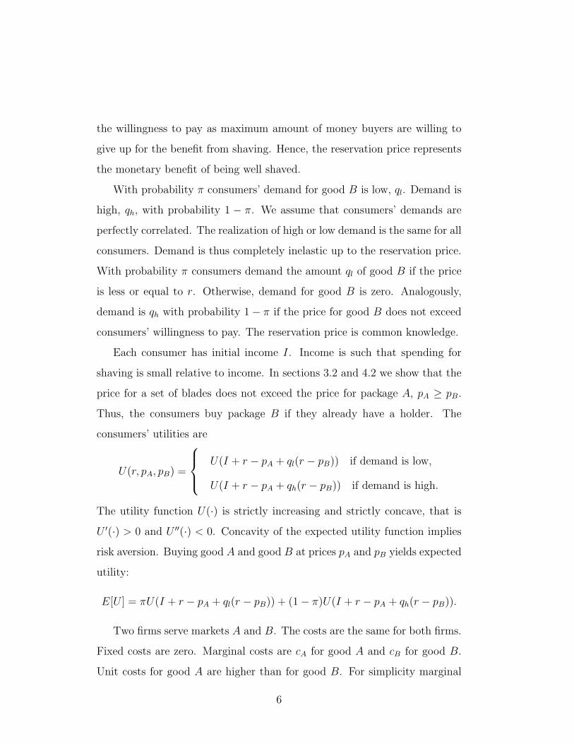
Let the arguments in the utility function be consumers’ wealth. If de-

mand is low, consumers’ wealth is higher under tying than under indepen-

dent pricing. However, if consumers have high demand, tie-in sales lead to

lower wealth than independent selling does. Hence, consumers enjoy higher

expected utility with tie-in sales if demand is low and expect lower utility if

demand is high. Figure 1 shows graphically that expected utility under ty-

ing lies above expected utility under independent pricing. Because expected

wealth is the same for the two selling regimes consumers have higher expected

utility under tying.

Expected Wealth x

U(x)

E[UIP]

E[UT]

Figure 1: Expected Utility

To see the tie-ins’ favorable effect for risk averse consumers let the con-

sumers’ wealth from a close and comfortable shave be lotteries. The lottery

under independent pricing LIP pays r − cA + ql(r − cB) with probability π

and r− cA + qh(r− cB) with probability 1−π. Tying is the lottery LT which

gives (1+ ql)(r−pTA) if demand is low and (1+ qh)(r−pT

A) if demand is high.

The expected value is the same for both lotteries. But the lotteries’ risks

measured by their variance differ. Since the tie-in price is higher than B’s

12

marginal costs the tying lottery exhibits a smaller variance.

V ar[LIP ] = (r − cB)2π(1− π)(qh − ql)2

> (r − pTA)2π(1− π)(qh − ql)

2 = V ar[LT ]

Since consumers are risk averse they are better off under tying. If the firms

tie their products, they set prices for the holder with blades below marginal

costs. For blades only, the price is above marginal costs. The consumers

benefit from the reduced good A price with certainty. Whereas the higher

blade prices adversely affect the buyers only with some probability. Tie-in

sales insure consumers against uncertain future demand.

4 Consumer Heterogeneity and a More Fun-

damental Utility Function

Hitherto, demand for package B is exogenous and the same for all consumers.

A more fundamental utility function endogenizes demand for B. This exten-

sion also entails that the demand in the second stage is no longer completely

inelastic. The strictly concave function U(·) defined on individuals’ incomes

and benefits from a clean shave exhibits risk aversion. However, the marginal

benefit from shaving decreases as the number of shaves increases. Consumers’

utility is

U(r, pA, pB) = U(I − pA + r ln(q + 1)− pBq),

where q is demand for blades only. Buying package A and q units of package

B renders benefit r ln(q + 1). The willingness to pay r ∈ [r, r] is a random

variable with uniform distribution. Consumers and firms both know the

reservation price’s density function f(r) = 1/(r− r). The reservation price’s

13

lower bound is greater than the marginal costs for A. This assumption en-

sures that consumers buy package A even if their demand for subsequent

blades was zero.

The game’s timing remains unchanged. Ex ante, the reservation price r

is unknown. The consumers learn their reservation price at the second stage,

after buying package A.

4.1 Independent Pricing

At the second stage consumers buy blades from the cheaper supplier because

they can freely combine handle and blades. Therefore, firms price B at

marginal costs. Given the prices for good B equal marginal costs, the firms

also charge marginal costs for good A in the first stage. Proposition 1 still

holds.

4.2 Tie-In Sales

After buying package A, consumers only demand blades at the second stage.

Knowing their reservation prices, consumers demand q units of package B.

Note that buyers used up package A’s blades. Thus, only shaves in the

second stage yield a benefit. A consumer with reservation price r demands

the amount q which maximizes his utility. Let q∗(r, pB) denote the consumers’

optimal demand for B at price pB depending on their willingness to pay:

q∗(r, pB) = arg maxq

U(I − pA + r ln(q)− pBq).

The first order condition for the consumers’ maximization problem deter-

mines the optimal demand q∗(r, pB) = r/pB. Because any critical point of a

concave function is a global maximizer, q∗(r, pB) is the optimal demand in

stage two for a consumer who is willing to pay r.

14

If the firms tie their goods, they have monopoly power in the second

stage. Like in section 3.2 two restrictions limit this monopoly power. First,

the firms do not price package B higher than package A. Secondly, buyers

still can change firms. Therefore, it is possible that firm j does not sell B

to all consumers who initially bought A from j. Consumers with j’s handle

buy good B from firm j or buy A and subsequent goods B from i. If the

consumers’ utility is higher in the latter case, they switch firm. Denote the

individual who is indifferent between staying at firm j and switching to firm

i by rj. Then, firm j supplies the set Rj of consumers. If firm j served the

fraction α of consumers in the first stage it’s maximization problem in the

second stage is:

maxpjB

α(pjB − cB)

∫

Rj

q∗ (r, pjB) f(r)dr

s.t.

pjB ≤ pTjA,

r ln(q∗(r, pjB))− (q∗(r, pjB)) pjB

≥ r ln(q∗(r, piB))− (q∗(r, piB)− 1) piB − pTiA.

Again, we show that the price for B equals the price for A. Consider the

firms’ no switching constraints for the indifferent consumers:

rj ln

(rj

pjB

)− rj = ri ln

(ri

piB

)− ri + piB − pT

iA

ri ln

(ri

piB

)− ri = rj ln

(rj

pjB

)− rj + pjB − pT

jA

The consumer with reservation price rj initially bought A from firm j and

is indifferent between buying q∗ sets of B from j and buying A plus q∗ − 1

sets of B from i. In the same way, the consumer with ri who first purchased

i’s holder is indifferent between staying with i and switching to firm j. We

15

next show that these indifferent consumers have the same willingness to pay,

rj = ri.

Assume the situation ri < rj. Further, suppose that consumers with

r > rj stay with firm j while consumers with r < ri stick to firm i as

depicted in figure 2. However, it is impossible then that consumers with

jrir r r

consumer r> jr stays at firm j

consumer r> ir switches from firm i to firm j consumer r< ir stays at firm i

consumer r< jr switches from firm j to firm i

Figure 2: Firms’ Indifferent Consumers with ri < rj

r ∈ [ri, rj] change from j to i while consumers with the same reservation

prices switch from i to j. Hence, ri ≥ rj.

Now assume ri > rj and consumers with r > rj stay with firm j while

consumers with r < ri stick to firm i. Figure 3 illustrates this situation.

Then, a consumer with reservation price ri who initially bought from firm

irjr r r

consumer r> jr stays at firm j

consumer r> ir switches from firm i to firm j

consumer r< ir stays at firm i

consumer r< jr switches

from firm j to firm i

Figure 3: Firms’ Indifferent Consumers with ri > rj

16

j has a higher utility than the indifferent consumer ri who initially bought

from firm i.

ri ln

(ri

pjB

)− ri > ri ln

(ri

piB

)− ri + piB − piA.

Obviously, r ln(r/pB) − r is decreasing in pB for all r. The consequence

is that firm i’s price for package B is higher than firm j’s price, pjB <

piB. Similarly, a consumer with willingness to pay rj who initially bought

from firm i must have a higher utility than the indifferent consumer rj. It

follows that piB < pjB which contradicts the first consequence and hence the

assumption ri > rj is not valid.

It follows from the analysis above that the firms’ indifferent consumers

have the same willingness to pay r. Substituting firm j’s LHS of the no-

switching condition into i’s RHS gives pTiA − piB = pjB − pT

jA. Only identical

prices for package A and B solve this equation, pTjA = pjB, j = 1, 2.

Given the pricing behavior at the second stage, the firms set prices for

good A at the first stage. Like in section 3.2, the firms use second stage

profits to subsidize price reductions for A to compete for demand. The firms

charge the price for handle with blades such that overall profits from selling

package A and B are zero. Accordingly, the price pjA solves the equation

πj = pjA − cA + (pjB − cB)E[q∗(r, pB)] = 0.

At the first stage, firm j expects demand E[q∗(r, pjB)] = (r + r)/(2pB) =

µr/pB for blades. Plugging consumers’ expected demand in firm j’s zero

profit condition and replacing blade price by the price for the access package

gives a quadratic equation in pjA. The solution for pjA ∈ R+ is:

pTjA = pT

jB =1

2cA − 1

2µr +

1

2

√(µr − cA)2 + 4µrcB.

17

Easy algebra shows that the price pTjA is always positive. Furthermore,

the price is smaller than package A’s marginal costs and greater than B’s

marginal costs. Finally, Proposition 2 still holds.

4.3 Comparison of Consumers’ Utility

Because demand for package B is not completely inelastic the effects from tie-

in sales are ambiguous. The utility function’s general form precludes a direct

comparison between expected utility under tying and independent pricing.

Therefore, we point out the combinations under which tie-ins provide the

buyers a higher expected utility.

Let the argument in the utility function be consumers’ wealth again.

Then, the selling scheme with higher expected wealth and lower variation

is superior. We first show that wealth’s variance under tying is lower than

under independent pricing. Then, we characterize the cost values for which

tying leads to higher wealth compared to marginal pricing.

In the following analysis we neglect the income I. Income is deterministic

and equal under the two selling schemes. The benefit from shaving in mon-

etary terms is a random variable W = r ln(r/pB + 1)− r − pA. The general

form for a random variables’ spread assigns wealth’s variance as

σ2W = E

[(r ln

(r

pB

+ 1

)− r

)2]−

(E

[r ln

(r

pB

+ 1

)− r

])2

.

Note that the variance is independent of A’s price. The consumers always

buy package A and know its price with certainty. So, pA has no effect on

wealth’s variance. Differentiating the variance with respect to the price pB

18

gives

∂σ2W

∂pB

=− 2E

[(r ln

(r

pB

+ 1

)− r

)r2

rpB + p2B

]

+ 2E

[r ln

(r

pB

+ 1

)− r

]

︸ ︷︷ ︸f(r)

E

[r2

rpB + p2B

]

︸ ︷︷ ︸g(r)

.

Denote the first term inside the expectation by f(r) and the second term

by g(r). The function g(r)’s derivative with respect to r is always positive.

Differentiating the other function f(r) makes

ln

(r

pB+ 1

)+

r

r + pB− 1.

If the price for package B equals the consumers’ willingness to pay, the dif-

ferential ∂f(r)/∂r is ln(2)+0.5r−1. We remember that the reservation price

is greater than one. The price for B is smaller than the willingness to pay.

Therefore, f(r) also increases in r. The Fortuin-Kasteleyn-Ginibre-inequality

states, for two increasing functions f and g and any random variable R, that

E[f(R)g(R)] ≥ E[f(R)]E[g(R)]. Applying this fact on the variance’s deriva-

tive shows that wealth’s variation does not depend positively on the price for

package B, ∂σ2W /∂pB ≤ 0. Under tying the price for blades is always higher

than under marginal pricing. Thus, the variation in consumers’ wealth de-

creases if firms tie their products.

To pin down the conditions under which tie-ins lead to higher utility

consider the consumers’ expected wealth

E[W ] = E

[r ln

(r

pB

+ 1

)]− µr − pA.

Bear in mind that prices satisfy the firms’ zero profit condition. Then, the

price for package A is a function of the price for package B, pA(pB) = cA −µr + µrcB/pB. Plugging in pA(pB) and differentiating expected wealth with

19

respect to pB is

1

p2B

(−E

[r2pB

r + pB

]+ µrcB

).

If ∂E[W ]/∂pB is positive, consumers expect higher wealth when the price

for B increases. On one hand, a reduction in the price for A has a positive

effect on wealth. On the other hand, the price reduction negatively effects

the monetary benefit from shaving. Consumers expect higher wealth if the

positive effect outweighs the negative,

µrcB ≥ E

[r2pB

r + pB

].

The adverse effect due to a price increase is highest for the willingness to

pay’s upper bound. Let then pB denote the price which solves the above

equation evaluated at r. Tie-in sales yield a higher expected wealth than

marginal pricing if the tying price pTA is smaller than this critical value pB:

pTA =

1

2cA − 1

2µr +

1

2

√c2A − 2cAµr + µ2

r + 4µrcB ≤ µrcBr

r2 − µrcB

= pB.

For all values cA which solve the above inequality pTA ≤ pB tie-in sales gen-

erate at least the same expected wealth as independent pricing does. The

upper bound for package A’s marginal costs is then

cA ≤ 3r2µrcB + µrr3 − µ2

rcBr − µ2rc

2B − r4

r(r − µrcB).

Marginal costs for A are greater than the costs for B. The upper limit for

package A’s marginal costs must also be greater than B’s marginal costs.

Solving cB < cA bounds cB above at r(r−µr)/µr. At last, consumers expect

higher wealth under tying if marginal costs are small enough, that is

cA ≤ 3r2µrcB + µrr3 − µ2

rcBr − µ2rc

2B − r4

r(r − µrcB),

cB < r(r − µr)/µr.

20

Yet, tie-in sales insure consumers against uncertainty. Under tying the

variation in wealth is smaller than under independent pricing. But expected

wealth can be higher if the firms price at marginal costs. Tie-in sales increase

the price for B. A higher price pB has two negative effects. First, the

spending for B increases and, second, the benefit from shaving decreases. The

positive effect due to a price decrease in good A does not always compensate

the negative effects in good B. Risk averse buyers account for expected

wealth and its variance. If marginal pricing leads to higher wealth the utility

function’s general form makes a clear statement impossible. The increase in

utility due to higher wealth can outweigh the utility decrease from a higher

variance. However, marginal costs small enough allow an assertion. In this

case, consumers prefer tie-in sales to independent pricing.

5 Conclusions

This paper introduces tie-in sales in a symmetric setting with price compe-

tition. We analyze the case of two firms. Each firm sells two goods. A good

example is the market for shaving systems. The razor basically consists of a

razor holder and blades. We compare the outcome under tie-in sales with the

benchmark independent pricing. If the firms do not tie, a firm’s own goods

are independent of each other. Under tying the firms design their products

such that their parts are not compatible with other firms’ components. Tie-

in sales allow the firms to create monopolies in one of the two markets. The

firms earn positive profits on the monopolized products. Because of compe-

tition in the market for the access good the firms drive each other down to

zero overall profits. They use the profits from monopolized goods to subsi-

dize losses in the competitive market. Although the firms tie their products,

21

the symmetry in the firms’ market power maintains price competition.

Beside the firms’ behavior we examine the effects from tie-in sales on

consumers’ expected utility. The buyers are uncertain about their future

spending. Before buying the holder, the consumers do not know their future

demand. In a simple model, risk averse consumers who are homogeneous

have completely inelastic demand. If demand is completely inelastic, tie-in

sales insure the buyers against uncertainty in expenditures. The consumers

prefer tie-in sales to independent pricing. We extend the simple model by

relaxing the assumption of completely inelastic demand and allowing for con-

sumer heterogeneity. In the extended version the tying’s effect is ambiguous.

Tie-in sales still have an insurance effect. But demand is no longer completely

inelastic and thus the benefits from shaving decrease under tie-in sales. How-

ever, we characterize cost combinations which lead to higher expected utility

under tie-in sales than under independent pricing.

22

References

[1] Adams, William James, Yellen, L. Janet, 1976, Commodity

Bundling and the Burden of Monopoly, The Quarterly Journal of Eco-

nomics, 90(3), pages 475-498.

[2] Burstein, L. Meyer, 1960, The Economics of Tie-In Sales, The Re-

view of Economics and Statistics, 42(1), pages 68-73.

[3] Burstein, L. Meyer, 1988, A Theory of Full-line Forcing, Studies

in banking theory, financial history and vertical control, New York, St.

Martin’s Press, pages 156-192.

[4] Carbajo, Jose, de Meza, David, Seidmann, J. Daniel, 1990, A

Strategic Motivation for Commodity Bundling, The Journal of Indus-

trial Economics, 38(3), pages 283-298.

[5] Chen, Yongmin, 1997, Equilibrium Product Bundling, The Journal

of Business, 70(1), pages 85-103.

[6] Economides, Nicholas, 1989, Desirability of Compatibility in the

Absence of Network Externalities, American Economic Review, 79(5),

pages 1165-1181.

[7] Kamecke, Ulrich, 1998, Tying Contracts and Asymmetric Informa-

tion, Journal of Institutional and Theoretical Economics, 154(3), pages

531-545.

[8] Liebowitz, J. Stan, 1983, Tie-In Sales and Price Discrimination, Eco-

nomic Inquiry, 21(3), pages 387-399.

23

[9] Lunn, John, 1990, Tie-In Sales and the Diffusion of New Technology,

Journal of Institutional and Theoretical Economics, 146(2), pages 249-

260.

[10] Matutes, Carmen, Regibeau, Pierre, 1988, “Mix and Match”:

Product Compatibility without Network Externalities, The RAND Jour-

nal of Economics, 19(2), pages 221-234.

[11] Matutes, Carmen, Regibeau, Pierre, 1992, Compatibility and

Bundling of Complementary Goods in a Duopoly, The Journal of Indus-

trial Economics, 40(1), pages 37-54.

[12] Whinston, D. Michael, 1990, Tying, Foreclosure, and Exclusion,

American Economic Review, 80(4), pages 837-859.

24