INSTITUTE OF PHYSICS PUBLISHING JOURNAL OF PHYSICS A: MATHEMATICAL AND GENERAL

J. Phys. A: Math. Gen. 39 (2006) 5563–5584 doi:10.1088/0305-4470/39/19/S14

On group Fourier analysis and symmetry preservingdiscretizations of PDEs

H Z Munthe-Kaas

Department of Mathematics, University of Bergen, Joh Brunsgt 12, N-5020, Norway

E-mail: hans@munthe-kaas.no

Received 12 October 2005, in final form 3 February 2006Published 24 April 2006Online at stacks.iop.org/JPhysA/39/5563

AbstractIn this paper we review some group theoretic techniques applied todiscretizations of PDEs. Inspired by the recent years active research inLie group- and exponential-time integrators for differential equations, wewill in the first part of the paper present algorithms for computing matrixexponentials based on Fourier transforms on finite groups. As an example,we consider spherically symmetric PDEs, where the discretization preservesthe 120 symmetries of the icosahedral group. This motivates the study ofspectral element discretizations based on triangular subdivisions. In thesecond part of the paper, we introduce novel applications of multivariatenon-separable Chebyshev polynomials in the construction of spectral elementbases on triangular and simplicial sub-domains. These generalized Chebyshevpolynomials are intimately connected to the theory of root systems and Weylgroups (used in the classification of semi-simple Lie algebras), and thesepolynomials share most of the remarkable properties of the classical Chebyshevpolynomials, such as near-optimal Lebesgue constants for the interpolationerror, the existence of FFT-based algorithms for computing interpolants andpseudo-spectral differentiation and existence of Gaussian integration rules. Thetwo parts of the paper can be read independently.

PACS numbers: 02.20.Qs, 02.30.Jr, 02.60.Jh

1. Introduction

As an introductory motivation, we briefly review some recent developments of numerical timeintegration based on computing exponentials. A detailed understanding of this introduction isnot necessary for reading the rest of the paper. Classical numerical integrators (e.g., Runge–Kutta and multistep) assumes an ODE y ′(t) = F(y(t)), where y(t) ∈ Rn and the basictime-step updates the solution are obtained by translations on Rn. Indeed all classical one-step

0305-4470/06/195563+22$30.00 © 2006 IOP Publishing Ltd Printed in the UK 5563

5564 H Z Munthe-Kaas

methods are of the form yn+1 = yn +�h,F (yn), where h denotes the timestep and �h,F is givenby the method.

In the last decade, there has been a significant development of numerical Lie groupintegrators (LGI) (Iserles et al 2000). These are based on the more general assumption thatthe domain of y(t) is a manifold M acted upon transitively by a Lie group G. Let g be thecorresponding Lie algebra and exp: g → G the exponential map. A vectorfield F on M canbe expressed in terms of a map A:M → g as F(y) = A(y) · y (Munthe-Kaas 1989). It isassumed that the group action p �→ exp(A) · p can be computed accurately and efficiently forall p ∈ M and A ∈ g. The basic time-step update in many LGI methods is obtained from thegroup action as yn+1 = exp(�h,A(yn)) ·yn, where �h,A(yn) ∈ g depends on the particular LGI.For matrix Lie groups, exp denotes the matrix exponential. As a simple example, considery ′(t) = A(y) · y, where A ∈ Rn×n, y ∈ Rn and the action is the matrix-vector product. Theexponentiated Euler method is the simplest possible LGI given as yn+1 = exp(hA(yn)) · yn. IfA is a skew-symmetric matrix, this yields a first-order integrator for equations evolving on asphere, where the update is done by the action of the orthogonal rotation matrix exp(hA). Theorder theory of high-order LGI is now well understood (Owren 2006). The basic differencebetween the classical-order theory and the order theory of LGI arises from the fact thattranslations on Rn form a commutative group, whereas more general group actions are non-commutative. Corrections for non-commutativity is necessary in any LGI of order higherthan 2.

LGI methods enjoy a number of nice geometrical properties, of which we will focus hereon their symmetry and equivariance properties. Fundamental in the theory of differentialequations is the equivariance of the solution curves with respect to any diffeomorphismφ:M → M acting on the domain. Let φ∗F denote the push forward of the vectorfield F, i.e.(φ∗F)(z) = T φ ·F(φ−1(z)) for all z ∈ M, where T φ denotes the tangent map (in coordinatesthe Jacobian matrix). Then the two differential equations y ′(t) = F(y(t)), y(0) = y0 andz′(t) = (φ∗F)(z(t)), z(0) = φ(y0) have analytical solution curves related by z(t) = φ(y(t)).In particular, if φ∗F = F , we say that φ is a symmetry of the vectorfield, and in that case φ

maps solution curves to other solution curves of the same equation.For numerical integrators, it is in general impossible to satisfy equivariance with respect

to arbitrary diffeomorphisms, since this would imply an analytically correct solution. (Therealways exists a local diffeomorphism which straighten the flow to a constant flow in x1

direction, and this is integrated exactly by any numerical method).The equivariance group of a numerical scheme is the largest group of diffeomorphisms

under which the numerical solutions transform equivariantly. It is known that the equivariancegroup of classical Runge–Kutta methods is the group of all affine linear transformations of Rn.LGI methods based on exact computation of exponentials have equivariance groups whichinclude the Lie group G on which the method is based, hence if some elements g ∈ G aresymmetries of the differential equation, then G-equivariant LGIs will exactly preserve thesesymmetries. However, if the exact exponential is replaced with approximations, care mustbe taken in order not to destroy G-equivariance and symmetry preservation of the numericalscheme. In the case of PDEs, symmetry preservation is also depending on symmetry preservingspatial discretizations.

In the recent years, there has been a significant interest in the application of LGI andother exponential-based integrators for solving PDEs (Hochbruck and Lubich 1998, Krogstad2005). A starting point for many of these methods are differential equations of the formu′(t) = L(u) + N (u), where L is a stiff linear differential operator, and N is a non-stiffand non-linear part of the PDE. In important cases, methods based on computing exp(L)

can replace implicit treatment of such stiff PDEs. Of particular interest to us in this paper

Symmetry preserving discretizations of PDEs 5565

are cases where L commutes with a group of symmetries, so that L(u ◦ g) = L(u) ◦ g for allg ∈ G. This is a typical situation for many differential operators arising from physical systems(e.g., the Laplace operator commutes with the group of Euclidean transformations of thedomain).

The paper is organized as follows. In section 2 we will discuss the use of Fourier transformson finite groups in the computation of the exponential of discretized linear operators commutingwith a finite group of domain symmetries. In particular, we will discuss the icosahedralsymmetry group, which is the largest finite subgroup of the full group of all rotations ofa sphere. In section 3 we will discuss issues related to spectral element discretizationswith icosahedral symmetries, in particular we will present a novel approach to constructinghigh-order bi-variate polynomial bases on triangles. This approach is based on the beautifulproperties of non-separable multivariate Chebyshev polynomials. These polynomials areconstructed by symmetric ‘caleidoscopic’ foldings of Fourier basis functions, and both thetheory and also practical computations (discretizations and FFTs) are depending on grouptheoretical ideas.

2. Symmetries and the matrix exponential

The topic of this section is applications of Fourier analysis on groups in the computationof matrix exponentials. Assuming that the domain is discretized with a symmetryrespecting discretization, we will show that by a change of basis derived from theirreducible representations of the group, the operator is block diagonalized. This simplifiesthe computation of matrix exponentials. The basic mathematics behind this chapter isrepresentation theory of finite groups (James and Liebeck 2001, Lomont 1959, Serre 1977).Applications of this theory in scientific computing is discussed by a number of authors, see e.g.Allgower et al (1992), Allgower et al (1998), Bossavit (1986), Douglas and Mandel (1992),Georg and Miranda (1992). Our exposition, based on the group algebra, is explained in detailin Ahlander and Munthe-Kaas (2005), which is intended to be a self-contained introductionto the subject.

2.1. G-equivariant matrices

A group is a set G with a binary operation g, h �→ gh, inverse g �→ g−1 and identity elemente, such that g(ht) = (gh)t, eg = ge = g and gg−1 = g−1g = e for all g, h, t ∈ G. We let |G|denote the number of elements in the group. Let I denote the set of indices used to enumeratethe nodes in the discretization of a computational domain. We say that a group G acts on a setI (from the right) if there exists a product (i, g) �→ ig : I × G → I, such that

ie = i for all i ∈ I, (1)

i(gh) = (ig)h for all g, h ∈ G and i ∈ I. (2)

The map i �→ ig is a permutation of the set I, with the inverse permutation being i �→ ig−1.An action partitions I into disjoint orbits

Oi = {j ∈ I | j = ig for some g ∈ G}, i ∈ I.

We let S ⊂ I denote a selection of orbit representatives, i.e. one element from each orbit.The action is called transitive if I consists of just a single orbit, |S| = 1. For any i ∈ I, welet the isotropy subgroup at i, Gi be defined as

Gi = {g ∈ G | ig = i}.

5566 H Z Munthe-Kaas

The action is free if Gi = {e} for every i ∈ I, i.e. there are no fixed points under the actionof G.

Definition 1. A matrix A ∈ CI×I is G-equivariant if

Ai,j = Aig,jg for all i, j ∈ I and all g ∈ G. (3)

The definition is motivated by the result that ifL is a linear differential operator commutingwith a group of domain symmetries G, and if we can find a set of discretization nodes I suchthat every g ∈ G acts on I as a permutation i �→ ig, thenL can be discretized as a G-equivariantmatrix A, see Allgower et al (1998), Bossavit (1986).

2.2. The group algebra

We will establish that G equivariant matrices are associated with (scalar or block) convolutionaloperators in the group algebra.

Definition 2. The group algebra CG is the complex vectorspace CG where each g ∈ Gcorresponds to a basis vector g ∈ CG. A vector a ∈ CG can be written as

a =∑g∈G

a(g)g where a(g) ∈ C.

The convolution product ∗ : CG × CG → CG is induced from the product in G asfollows. For basis vectors g,h, we set g ∗ h ≡ gh, and in general if a = ∑

g∈G a(g)gand b = ∑

h∈G b(h)h, then

a ∗ b =∑

g∈Ga(g)g

∗(∑

h∈Gb(h)h

)=

∑g,h∈G

a(g)b(h)(gh) =∑g∈G

(a ∗ b)(g)g,

where

(a ∗ b)(g) =∑h∈G

a(gh−1)b(h) =∑h∈G

a(h)b(h−1g). (4)

Consider a G-equivariant A ∈ Cn×n in the case where G acts freely and transitively onI. In this case there is only one orbit of size |G| and hence I may be identified with G.Corresponding to A there is a unique A ∈ CG, given as A = ∑

g∈G A(g)g, where A is thefirst column of A, i.e.

A(gh−1) = Agh−1,e = Ag,h. (5)

Similarly, any vector x ∈ Cn corresponds uniquely to x = ∑g∈G x(g)g ∈ CG, where

x(g) = xg for all g ∈ G. Consider the matrix vector product

(Ax)g =∑h∈G

Ag,hxh =∑h∈G

A(gh−1)x(h) = (A ∗ x)(g).

If A and B are two equivariant matrices, then AB is the equivariant matrix where the firstcolumn is given as

(AB)g,e =∑h∈G

Ag,hBh,e =∑h∈G

A(gh−1)B(h) = (A ∗ B)(g).

We have shown that if G acts freely and transitively, then the algebra of G-equivariant matricesacting on Cn is isomorphic to the group algebra CG acting on itself by convolutions from theleft.

Symmetry preserving discretizations of PDEs 5567

In the case where A is G-equivariant w.r.t. a free, but not transitive, action of G on I,we need a block version of the above theory. Let Cm×�G ≡ Cm×� ⊗ CG denote the space ofvectors consisting of |G| matrix blocks, each block of size m × �, thus A ∈ Cm×�G can bewritten as

A =∑g∈G

A(g) ⊗ g where A(g) ∈ Cm×�. (6)

The convolution product (4) generalizes to a block convolution ∗ : Cm×�G × C�×kG →Cm×kG given as

A ∗ B =∑

g∈GA(g) ⊗ g

∗(∑

h∈GB(h) ⊗ h

)=

∑g∈G

(A ∗ B)(g) ⊗ g,

where

(A ∗ B)(g) =∑h∈G

A(gh−1)B(h) =∑h∈G

A(h)B(h−1g), (7)

and A(h)B(h−1g) denotes a matrix product.If the action of G on I is free, but not transitive, then I split in m orbits, each of size |G|. We

letS denote a selection of one representative from each orbit. We will establish an isomorphismbetween the algebra of G-equivariant matrices acting on Cn and the block-convolution algebraCm×mG acting on CmG. We define the mappings µ : Cn → CmG, ν : Cn×n → Cm×mG as

µ(y)i(g) = yi(g) = yig ∀i ∈ S, g ∈ G, (8)

ν(A)i,j (g) = Ai,j (g) = Aig,j ∀i, j ∈ Sg ∈ G. (9)

In Ahlander and Munthe-Kaas (2005) we show:

Proposition 1. Let G act freely on I. Then µ is invertible and ν is invertible on the subspaceof G-equivariant matrices. Furthermore, if A,B ∈ Cn×n are G-equivariant and y ∈ Cn, then

µ(Ay) = ν(A) ∗ µ(y), (10)

ν(AB) = ν(A) ∗ ν(B). (11)

To complete the connection between G-equivariance and block convolutions, we need toaddress the general case where the action is not free, hence some of the orbits in I have reducedsize. One way to treat this case is to duplicate the nodes with non-trivial isotropy subgroups,thus a point j ∈ I is considered to be |Gj | identical points, and the action is extended to afree action on this extended space. Equivariant matrices on the original space is extended byduplicating the matrix entries, and scaled according to the size of the isotropy. We define

µ(x)i(g) = xi(g) = xig ∀i ∈ S, g ∈ G, (12)

ν(A)i,j (g) = Ai,j (g) = 1

|Gj |Aig,j ∀i, j ∈ Sg ∈ G. (13)

With these definitions it can be shown that (10) and (11) still hold. It should be noted that µ

and ν are no longer invertible, and the extended block convolutional operator ν(A) becomessingular. This poses no problems for the computation of exponentials since this is a forwardcomputation. Thus we just exponentiate the block convolutional operator and restrict the resultback to the original space. However, for inverse computations such as solving linear systems,the characterization of the image of µ and ν as subspaces of CmG and Cm×mG is an importantissue for finding the correct solution (Ahlander and Munthe-Kaas 2005, Allgower et al 1993).

5568 H Z Munthe-Kaas

2.3. The generalized Fourier transform (GFT)

So far we have argued that a symmetric differential operator becomes a G-equivariant matrixunder discretization, which again can be represented as a block convolutional operator. Inthis section we will show how convolutional operators are block diagonalized by a Fouriertransform on G. This is the central part of Frobenius’ theory of group representations from1897–1899. We recommend the monographs (Fassler and Stiefel 1992, James and Liebeck2001, Lomont 1959, Serre 1977) as introductions to representation theory with applications.

Definition 3. A d-dimensional group representation is a map R : G → Cd×d such that

R(gh) = R(g)R(h) for all g, h ∈ G. (14)

Generalizing the definition of Fourier coefficients, we define for any A ∈ Cm×kG and anyd-dimensional representation R a matrix A(R) ∈ Cm×k ⊗ Cd×d as

A(R) =∑g∈G

A(g) ⊗ R(g). (15)

Proposition 2 (The convolution theorem). For any A ∈ Cm×kG, B ∈ Ck×�G and anyrepresentation R, we have

(A ∗ B)(R) = A(R)B(R). (16)

Proof. The statement follows from

A(R)B(R) =∑

g∈GA(g) ⊗ R(g)

(∑h∈G

B(h) ⊗ R(h)

)

=∑

g,h∈GA(g)B(h) ⊗ R(g)R(h) =

∑g,h∈G

A(g)B(h) ⊗ R(gh)

=∑

g,h∈GA(gh−1)B(h) ⊗ R(g) = (A ∗ B)(R).

�

Let dR denote the dimension of the representation. For use in practical computations, itis important that A ∗ B can be recovered by knowing (A ∗ B)(R) for a suitable selection ofrepresentations, and furthermore that their dimensions dR are as small as possible. Note thatif R is a representation and X ∈ CdR×dR is non-singular, then also R(g) = XR(g)X−1 is arepresentation. We say that R and R are equivalent representations. If there exists a similaritytransform R(g) = XR(g)X−1, such that R(g) has a block diagonal structure, independent ofg ∈ G, then R is called reducible, otherwise it is irreducible.

Theorem 3 (Frobenius). For any finite group G there exists a complete list R of non-equivalentirreducible representations, such that∑

R∈Rd2

R = |G|.

Defining the GFT for a ∈ CG as

a(R) =∑g∈G

a(g)R(g) for every R ∈ R, (17)

Symmetry preserving discretizations of PDEs 5569

Table 1. Gain in computational complexity for matrix exponential via GFT.

Domain G |G| {dR}R∈R Wdirect/Wfspace

Triangle D3 6 {1, 1, 2} 21.6Tetrahedron S4 24 {1, 1, 2, 3, 3} 216Cube S4 × C2 48 {1, 1, 1, 1, 2, 2, 3, 3, 3, 3} 864Icosahedron A5 × C2 120 {1, 1, 3, 3, 3, 3, 4, 4, 5, 5} 3541

we may recover a by the inverse GFT (IGFT)

a(g) = 1

|G|∑R∈R

dR trace(R(g−1)a(R)). (18)

For the block transform of A ∈ Cm×kG given in (15), the GFT and the IGFT are givencomponentwise as

Ai,j (R) =∑g∈G

Ai,j (g)R(g) ∈ CdR×dR , (19)

Ai,j (g) = 1

|G|∑R∈R

dR trace(R(g−1)Ai,j (R)). (20)

Complete lists of irreducible representations for a selection of common groups are found inLomont (1959).

2.4. Applications to the matrix exponential

We have seen that via the GFT, any G-equivariant matrix is block diagonalized. Correspondingto an irreducible representation R, we obtain a matrix block A(R) of size mdR × mdR , wherem is the number of orbits in I and dR the size of the representation. Let Wdirect denotethe computational work, in terms of floating point operations, for computing the matrixexponential on the original data A, and let Wfspace be the cost of doing the same algorithmon the corresponding block diagonal GFT-transformed data A. Thus Wdirect = c(m|G|)3 =cm3

(∑R∈R d2

R

)3,Wfspace = cm3 ∑

R∈R d3R and the ratio becomes

O(n3): Wdirect/Wfspace =(∑

R∈Rd2

R

)3 / ∑R∈R

d3R.

Table 1 lists this factor for the symmetries of the triangle, the tetrahedron, the 3D cube and themaximally symmetric discretization of a 3D sphere (icosahedral symmetry with reflections).

The cost of computing the GFT is not taken into account in this estimate. There existsfast GFT algorithms of complexity O(|G| log�(|G|)) for a number of groups, but even if we usea slow transform of complexity O(|G2|), the total cost of the GFT becomes just O(m2|G|2),which is much less than Wfspace.

2.4.1. Example: Equilateral triangle. The smallest noncommutative group is D3, thesymmetries of an equilateral triangle. There are six linear transformations that map thetriangle onto itself, three pure rotations and three rotations combined with reflections. Infigure 1(a), we indicate the two generators α (rotation 120◦ clockwise) and β (right–leftreflection). These satisfy the algebraic relations α3 = β2 = e, βαβ = α−1, where e denotesthe identity transform. The whole group is D3 = {e, α, α2, β, αβ, α2β}.

Given an elliptic operator L on the triangle such that L(u ◦ α) = L(u) ◦ α and L(u ◦ β) =L(u) ◦ β for any u satisfying the appropriate boundary conditions on the triangle, let the domain

5570 H Z Munthe-Kaas

β

α

1

3

5

2

4

6

89

7

10

(a) (b)

Figure 1. Equilateral triangle with a symmetry preserving set of ten nodes.

Table 2. A complete list of irreducible representations for D3.

α β

ρ0 1 1ρ1 1 −1

ρ2

(−1/2 − √3/2√

3/2 − 1/2

) ( 1 00 − 1

)

be discretized with a symmetry respecting discretization, see figure 1(b). In this example weconsider a finite difference discretization represented by the nodes I = {1, 2, . . . , 10}, suchthat both α and β map nodes to nodes. In finite element discretizations, one would use basisfunctions mapped to other basis functions by the symmetries. We define the action of D3

on I as

(1, 2, 3, 4, 5, 6, 7, 8, 9, 10)α = (5, 6, 1, 2, 3, 4, 9, 7, 8, 10),

(1, 2, 3, 4, 5, 6, 7, 8, 9, 10)β = (2, 1, 6, 5, 4, 3, 7, 9, 8, 10),

and extend to all of D3 using (2). As orbit representatives, we may pick S = {1, 7, 10}. Theaction of the symmetry group is free on the orbit O1 = {1, 2, 3, 4, 5, 6}, while the points in theorbit O7 = {7, 8, 9} have isotropy subgroups of size 2, and finally O10 = {10} has isotropy ofsize 6.

The operator L is discretized as a matrix A ∈ C10×10 satisfying the equivariancesAig,jg = Ai,j for g ∈ {α, β} and i, j ∈ S. Thus we have e.g. A1,6 = A3,2 = A5,4 =A4,5 = A2,3 = A6,1.

D3 has three irreducible representations given in table 2 (extended to the whole groupusing (14)). To compute exp(A), we find A = ν(A) ∈ C3×3G from (13) and findA = GFT(A) from (19). The transformed matrix A has three blocks, A(ρ0), A(ρ1) ∈ Cm×m

and A(ρ2) ∈ Cm×m ⊗ C2×2 � C2m×2m, where m = 3 is the number of orbits. We exponentiateeach of these blocks, and find the components of exp(A) using the inverse GFT (20).

We should remark that in Lie group integrators, it is usually more important to computey = exp(A) · x for some vector x. In this case, we compute y(ρi) = exp(A(ρi)) · x(ρi), andrecover y by the inverse GFT. Note that x(ρ2), y(ρ2) ∈ Cm ⊗ C2×2 � C2m×2.

2.4.2. Example: Icosahedral symmetry. As a second example illustrating the general theory,we solve the simple heat equation

ut = ∇2u

Symmetry preserving discretizations of PDEs 5571

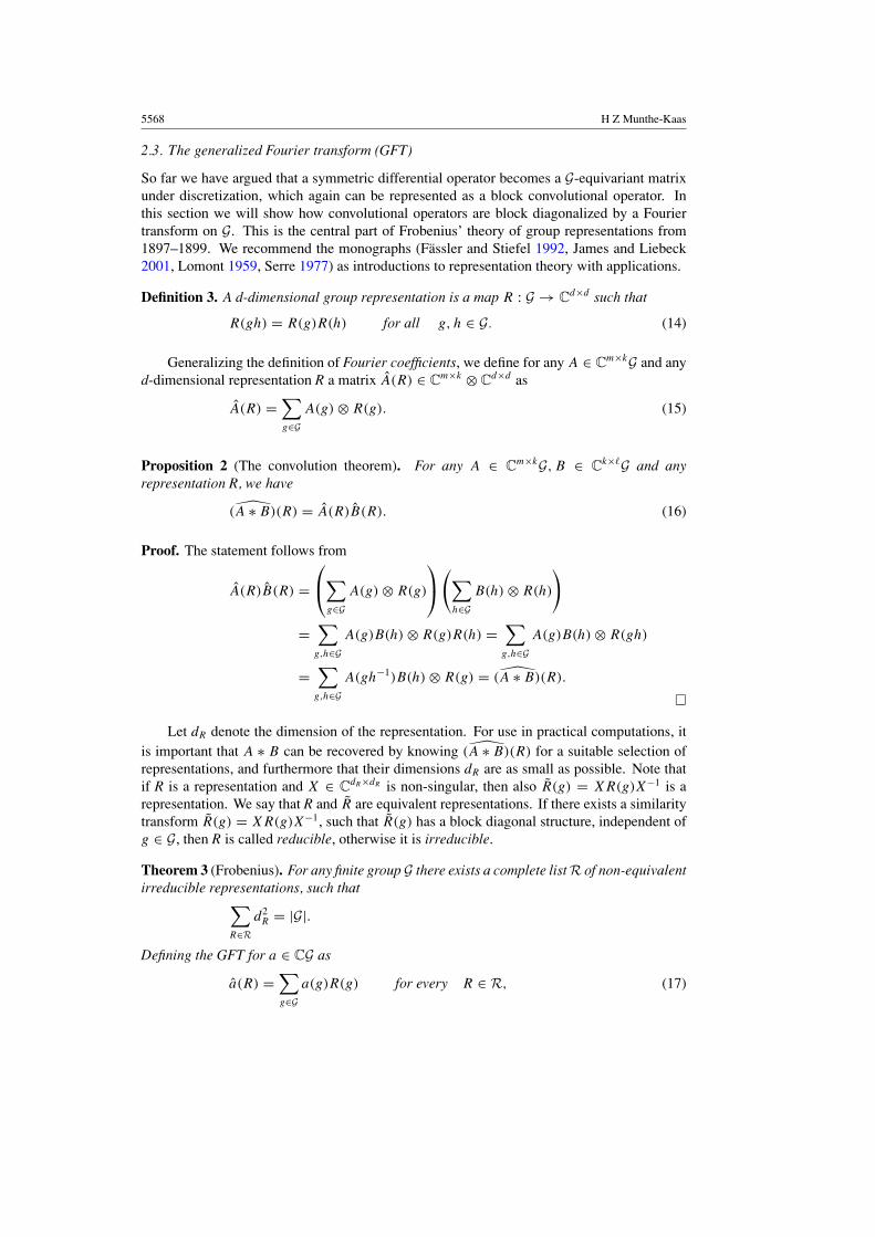
on the surface of a unit sphere. The programming in this example is done by Trønnes (2005)in his master thesis.

The sphere is divided into 20 equilateral triangles, and each triangle subdivided in a finitedifference mesh respecting all the 120 symmetries of the full icosahedral symmetry group(including reflections). To understand this group, it is useful to realize that five tetrahedra canbe simultaneously embedded in the icosahedron, so that the 20 triangles correspond to thein total 20 corners of these five tetrahedra. From this one sees that the icosahedral rotationgroup is isomorphic to A5, the group of all 60 even permutations of the five tetrahedra. The3D reflection matrix −I obviously commutes with any 3D rotation, and hence we realizethat the full icosahedral group is isomorphic to the direct product C2×A5, where C2 = {1,−1}.The irreducible representations of A5, listed in Lomont have dimensions {1, 3, 3, 4, 5}, andthe representations of the full icosahedral group are found by taking tensor products of thesewith the two one-dimensional representations of C2. The fact that the full icosahedral groupis a direct product is also utilized in faster computation of the GFT. This is, however, not ofmajor importance, since the cost of the GFT in any case is much less than the cost of thematrix exponential.

The figures below show the solution of the heat equation at times 0, 2, 5, 10, 25 and 100.The initial condition consists of two located heat sources in the northern hemisphere.

5572 H Z Munthe-Kaas

This example serves as a simple toy example to check the practical issues of programmingthe group-based diagonalization techniques discussed above. In future work, we aim atsolving more interesting equations such as shallow water equations and Euler flow equationson spherical geometries, using high-order Lie group integrators for the time integration andhigh-order spectral element discretizations in the space. For this purpose, we are interestedin spectral element methods based on triangular subdivisions. In the remaining part of thispaper, we will overview a novel approach to this topic, based on families of non-separablemultivariate Chebyshev polynomials obtained from group theory.

3. Multivariate Chebyshev and triangular spectral elements

Bivariate Chebyshev polynomials were constructed independently by Koornwinder (1974)and Lidl (1975) by folding exponential functions. Multidimensional generalizations (the A2

family) appeared first in Eier and Lidl (1982). In Hoffman and Withers (1988), a generalfolding construction was presented. Characterization of such polynomials as eigenfunctionsof differential operators is found in Beerends (1991), Koornwinder (1974). Although thefundamental mathematical properties of multivariate Chebyshev polynomials are developedin the above papers, they are to our knowledge not appearing in any works on numericalanalysis, approximation theory nor any other areas of computational science. It is our goalto show that these polynomials have significant roles to play in computations, similar to thefamous univariate case. A more detailed exposition of the theory of this paper will appear inMunthe-Kaas (2006).

3.1. Multivariate Chebyshev polynomials: a general construction

To motivate a general construction of multivariate Chebyshev polynomials, we consider theclassical univariate case obtained by ‘folding’ the exponential functions to cosine functions,and applying a change of variables to turn cosine functions into Chebyshev polynomials.Define the Fourier basis functions (k, θ) = exp(2πikθ) for θ ∈ G = R/Z = [0, 1) andk ∈ G = Z. Let W = {1,−1} be a symmetry group acting on G, and consider the ‘folded’exponentials

(k, θ)s = 1

|W |∑γ∈W

(k, γ θ) = 1

|W |∑γ∈W

(γ k, θ) = 1

2((k, θ) + (−k, θ)) = cos(2πkθ).

Define the change of variables x(θ) = (1, θ)s = cos(2πθ). This defines Chebyshevpolynomials Tk(x) = (k, θ)s for k = {0, 1, . . .}. Note that T0(x) = 1 and T1(x) = x. The factthat all Tk(x) are polynomials follows from the recursion 2T1(x) · Tk(x) = Tk+1(x) + Tk−1(x),which is a special case of (29). It should be noted that the beautiful computational properties ofChebyshev polynomials, such as existence of FFT-based fast algorithms, recursion relations,orthogonality (continuous and discrete) and excellent interpolation properties can all beexplained in terms of group theory and can be generalized to multivariate cases.

Let G = Rd/Zd denote a d-dimensional domain, one-periodic in each direction, thus〈G, +〉 is an Abelian (commutative) group where + denotes componentwise addition modulo1. Let G = Zd denote the Abelian group of d-dimensional integer vectors, and define the dualpairing (·, ·): G×G → C as

(k, θ) = exp(2π ikT θ) (21)

satisfying

(k, θ + θ ′) = (k, θ) · (k, θ ′), (k + k′, θ) = (k, θ) · (k′, θ). (22)

Symmetry preserving discretizations of PDEs 5573

Note that {(k, ·): k ∈ G} is the Fourier basis on G (a complete list of irreduciblerepresentations), while {(·, θ): θ ∈ G} is the Fourier basis on G, thus G and G are dualAbelian groups (Rudin 1962).

Let W ⊂ Zd×d be a finite group of integer matrices, defining a left action θ �→ γ θ on Gand a right action kT �→ kT γ on G. Define the symmetrized Fourier basis

(k, θ)s = 1

|W |∑γ∈W

(k, γ θ) = 1

|W |∑γ∈W

(γ T k, θ), (23)

and introduce a change of variables

xj (θ) = (ej , θ)s, (24)

where ej = (0, . . . , 1, . . . , 0)T and j ∈ {1, . . . , d}. We define a family of functions

Tk(x) = (k, θ)s for k ∈ G. (25)

We will impose enough structure on W to ensure that Tk(x) form a complete family of d-variatepolynomials, which we will call the multivariate Chebyshev polynomials associated with W .

First some properties that hold regardless of W . From the definition it follows immediatelythat Tk(x) satisfy

T0(x) = 1 (26)

Tej(x) = xj (27)

Tk(x) = Tγ T k(x) for all γ ∈ W . (28)

The mother of all recurrence relations between Tk(x) is the following:

Tk(x)T�(x) =∑m∈G

αk,�(m)Tm(x) =∑m∈S

|mT W |αk,�(m)Tm(x), (29)

where S denotes a selection of one element from each orbit of W in G and |mT W | denotesthe size of the orbit represented by m ∈ S. The function α is given by a convolution

αk,�(m) = 1

|W |2∑ ∑

γ,η∈W

δγ T k+ηT �,m, (30)

where δ is the Kronecker-δ. To understand (29), recall the convolution formula for the(Abelian) Fourier transform (fg)(k) = (f ∗ g)(k) = ∑

m∈G f (k−m)g(m), where f, g ∈ CG

and f , g ∈ CG. The Fourier transform of Tk(x(θ)) is

T k(m) = 1

|W |∑γ∈W

δγ T k,m,

and by defining

αk,�(m) = TkT�(m) = (Tk ∗ T�)(m), (31)

we obtain (30). Due to symmetry, it is sufficient to sum over just one element in each W-orbitand scale with the size of the orbit.

The reader is encouraged to verify that (29) implies the common recurrence amongclassical Chebychev polynomials in the case where d = 1 and W = {1,−1}.

A trivial example of these formulae is obtained when d = 1 and W = {1}. In this case weget x = exp(2πiθ), Tk(x) = xk for k ∈ Z, and (29) becomes Tk(x) · T�(x) = Tk+�(x). ThusTk are not polynomials when k < 0, because W is too small and lacks symmetries sendingnegative k to positive. On the other hand, if W is too large, then {Tk(x)} may not generate thefull space of all multivariate polynomials, but just certain linear combinations of these.

In the following section we will introduce the Weyl groups W associated with root systems.These groups are just the right size to guarantee that {Tk(x): k ∈ S} form complete bases forthe space of multivariate polynomials.

5574 H Z Munthe-Kaas

3.2. Root systems and Weyl groups

A root system is a subset of a Euclidean space E = Rd such that

(i) is finite, spans E and does not contain 0.(ii) If α ∈ then the only multiples of α in are ±α.

(iii) If α ∈ then the reflection σα = I − 2ααT

αT αleaves invariant.

(iv) If α, β ∈ then 2 αT β

αT α∈ Z.

The (finite) group generated by the reflections W = 〈σα | α ∈ 〉 is called the Weyl group.The integer linear combination of all the roots α ∈ is called the root lattice �r . The affineWeyl group is the group generated by W and all the translations in the root lattice.

A root system always has a basis, defined as d linearly independent vectors {α1, . . . , αd} ⊂ so that any α ∈ can be written as α = ∑d

j=1 cjαj , where cj ∈ Z are either all non-negativeor all non-positive. αj are called the simple roots. We let

A = (α1, . . . , αd)

denote the matrix with columns formed by the simple roots, hence �r = {A · κ: κ ∈ Zd}.Given any lattice � ⊂ Rd , we define the dual lattice �⊥ ⊂ Rd as the set of all vectors

whose inner-product with vectors in � yield integer values, thus �⊥r = {A−T · κ: κ ∈ Zd}. A

well-known result of Fourier analysis is that periodization of Rd with respect to a lattice � isequivalent to restricting the Fourier coefficients to the dual lattice �⊥.

According to the general construction of section 3.1, we construct the Chebyshevpolynomials Tk(x) from as follows:

• Primal and dual spaces: The root lattice �r defines a periodic domain Rd/�r . Via thebasis A for �r , this domain is isomorphic to G = Rd/Zd . Using the dual basis A−T , theFourier space becomes G = Zd .

• Weyl group: Using the A basis, the group W becomes a group of integer matrices actingon G. We find σαi

A = Aσi , where σi is the integer matrix

σi = I − eieTi C,

and C is the Cartan matrix of the root system, defined as

Cj,� = 2αT

j α�

αTj αj

.

Thus, from the Cartan matrix of the root system, we immediately find the integer matrices{σi}di=1 generating the Weyl group W . Given W , we construct the Chebyshev family{Tk(x): k ∈ S}.

• Fundamental domain in G: It can be shown that a selection of orbit representatives canalways be taken as the first quadrant of G = Zd , i.e.

S = {k ∈ Zd : ki � 0 for all i}.Furthermore, there exists a partial ordering ≺ on S such that the monomials can be writtenas

xk = xk11 · · · xkd

d = ckTk(x) +∑�∈S�≺k

c�T�(x) for ck, c� ∈ C, ck �= 0 .

Hence {Tk(x): k ∈ S} is a basis for the space of multivariate polynomials.

Symmetry preserving discretizations of PDEs 5575

• Fundamental domain in G: Let � denote the fundamental domain of W acting on G.The domain � has a simple characterization in terms of A and C. If the root system isirreducible, then � is always a simplex, and for reducible root systems, � becomes aCartesian product of the fundamental domains for each of the irreducible components of , see Munthe-Kaas (2006) for details. It can be shown that the coordinate map θ �→ x

is invertible between � and the codomain δ = x(�). The Jacobian of x(θ) is nonsingularinside � and singular on the boundary. It is important to note that while � are simplexes,this is not the case for the transformed domain δ = x(�). This poses challenges for theconstruction of spectral element bases that we will address in the case A2 in section 3.4.

• Continuous orthogonality: The exponentials are orthogonal under the standard innerproduct on G, and therefore the symmetrized exponentials are orthogonal on �. Thus theChebyshev polynomials satisfy a continuous orthogonality∫

δ

Tk(x) · T�(x)ω(x) dx = 0 for k, � ∈ S, k �= �,

where ω(x) is the Jacobian determinant of the coordinate map x(θ). For the 1D case,ω(x) = (2π

√1 − x2)−1 (the normal Chebyshev weight function scaled with 2π ).

• Discrete orthogonality: For fast computations, it is important to find a good discretizationof � ⊂ G. Up to a band-limit, the exponentials (k, θ) are orthogonal with on a uniformlattice in G, and uniform lattices provide Gaussian integration rules for the exponentials(with equal Gaussian weights). For the symmetrized exponentials, we need a latticewhich is invariant under W . One such lattice with maximal symmetries is obtained bydownscaling the root lattice with an integer factor m = k|C|. We include the determinantof the Cartan matrix to ensure that the lattice contains both the root lattice, and also theweights lattice, which are all the points with maximal symmetry under the action of theaffine Weyl group on Rd (Humphreys 1970). Let �m ⊂ G denote the down-scaled rootlattice, restricted to �. Since G is expressed in terms of the basis A, this becomes

�m ={θ ∈ �: θ = κ

m, κ ∈ Zd

}.

The symmetrized exponentials (k, θ)s satisfy a discrete orthogonality on �m, where theGaussian weight in a point θ is proportional to the size of the orbit |Wθ |. Thus theChebyshev polynomials satisfy orthogonality under the discrete inner product

〈Tk(x), T�(x)〉m = 1

c

∑θ∈�m

|Wθ | · Tk(x(θ)) · T�(x(θ)),

where c = |W |∑θ∈�m|Wθ |. The Gaussian quadrature formula∫

x∈δ

f (x)ω(x) dx ≈ c∑θ∈�m

|Wθ |f (x(θ))

is exact whenever f (x) = Tk(x), k �= mκ for some 0 �= κ ∈ Zd . The formula fails if k isin the dual lattice (�r/m)⊥, except k = 0, since these Tk alias to T0 on �m. It should benoted that our lattice �m is a generalization of Chebyshev–Gauss–Lobatto points in 1D(i.e., Chebyshev extremal points, with half weights on the boundary points). We can alsogeneralize Chebyshev–Gauss points (zeros of Chebyshev polynomials) by using latticesobtained by taking appropriate cosets of the downscaled root lattice.

To complete this section, we want to characterize all root systems, and present theirreducible cases in 2D. A root system is called reducible, if the roots can be separated intotwo sets, such that the roots in one subset is orthogonal to all the other roots. Any root

5576 H Z Munthe-Kaas

Figure 2. Dynkin diagrams.

system can be decomposed into irreducible components, and it is sufficient to study these. If aroot system can be decomposed, then the corresponding fundamental domains become tensorproducts of the corresponding irreducible subdomains, and all the Chebyshev polynomialsbecome tensor products of Chebyshev polynomials on the irreducible components. Thusthe standard construction of the tensor product Chebyshev bases on box-shaped domainscorresponds to a root system which can be completely decomposed into 1D roots.

Irreducible root systems are uniquely characterized in terms of their Dynkin diagrams,figure 2. These diagrams have one node for each simple root αj ∈ �. The only possibleangles between the simple roots are 90◦, 60◦, 45◦ or 30◦. We draw no line between the nodesif the corresponding simple roots are orthogonal, one line if the angle is 60◦, two lines for 45◦

and three lines for 30◦. Roots may come in different lengths, but in an irreducible root system,there are at most two different lengths of the roots. To indicate short and long roots an arrowis inserted in the diagram, thus on the left of < are the short roots, on the right the long ones.The 2D irreducible root systems are shown in figure 3.

The sequence of diagrams A1, A2, A3,D4,D5, E6, E7 and E8 are of particular interestin sampling theory. The root lattices corresponding to these are known to be the densestlattice packings in spaces of dimensions 1–8 (Conway and Sloane 1988). Suppose we seek asampling lattice A on Rd so that the Euclidean distance in the Fourier space between 0 and theclosest non-zero point in the dual lattice A⊥ is some given constant c, i.e. we seek a samplingexact on ‖k‖2 < c band limited functions. How can we choose such a lattice A with the lowestsampling density? The solution is: choose a lattice from the sequence above! To explainthis, we note that all these lattices are self-dual (dual of same type). In the Fourier space,maximizing grid density |A−T |−1 (for a given lattice constant c) is equivalent to minimizingthe density |A|−1 in primal space. For dimensions 2, 3, 4 and 5, going from a rectangular tooptimal grid saves 13%, 29%, 50% and 65% of the gridpoints.

3.3. Chebyshev expansions and symmetric FFTs

The (infinite) Chebychev expansion of a well-behaved function f (x) defined for x ∈ δ isgiven as

f (x) =∑k∈S

|kT W |f (k)Tk(x),

where f ∈ CG is the Fourier transform of f (x(θ)) considered as a symmetric function inCG. If we restrict x to the finite set {x(θ): θ ∈ �m}, then we obtain a finite interpolatingChebyshev series of the form

Symmetry preserving discretizations of PDEs 5577

Rootsystem B2Rootsystem A2

Rootsystem G2

Figure 3. Irreducible root systems in 2D. The irreducible 2D root systems given by A2, B2 andG2, corresponding to fundamental domains � ⊂ G given as equilateral triangle, 45◦ − 45◦ − 90◦triangle and 30◦ − 60◦ − 90◦ triangle (yellow colour). Blue dots are the roots, blue arrows thesimple roots, red dots the weights lattice and red arrows the fundamental dominant weights, thedotted lines are the mirrors in the affine Weyl group and the black dots indicate a downscaling ofthe root lattice by a factor m = 12. The parallelograms show the periodicity of the root lattice, andhence the fundamental domain of the (unsymmetrized) Fourier basis.

f (x(θ)) =∑k∈Sm

|kT W |f (k)Tk(x(θ)).

Sampling at m-downscaled root lattice can be described as going from the continuous Abeliangroup G to the finite subgroup Gm = Zd

m. In the Fourier space, the sampling is describedby going from the infinite group G to the finite quotient Gm = G/mG � Zd

m. The finite set

5578 H Z Munthe-Kaas

Sm ⊂ S denotes the fundamental domain of the right action of W on Gm, see Munthe-Kaas(2006) for details.

Computationally the discrete Chebyshev interpolation problem is solved by computing asymmetric discrete Fourier transform f �→ f . A simple solution to this problem is just toform the full symmetrized f ∈ CGm, computing f with a standard FFT, and restrict the resultto Sm. The cost is 5N log2(N) real flops, where N = md .

In Munthe-Kaas (1989), we provide group theoretic symmetric FFTs that can utilize allthe symmetries in W and real symmetry in f . A related approach is found in Puschel andRotteler (2004). A group theoretical explanation of the classical Cooley–Tukey algorithm isthe result that if H < G (subgroup of Abelian group) then H = G/H⊥. So, the Cooley–Tukeyalgorithm can be generalized to any subgroup decomposition. The sequence

G|C| < G2|C| < · · · < G2k |C|

preserves all the symmetries in W . Symmetries may be lost in the cosets, but in that case twodifferent cosets will be identified by a symmetry. By carefully using all the symmetries bothin primal space and in the Fourier space, we obtain an algorithm saving a factor 2|W | bothin flops and in storage with respect to the full non-symmetric complex FFT. The cost of thesymmetrized algorithm is 5

2M log2(M), where M = |�m| is the number of lattice points inthe fundamental domain.

3.4. The Chebyshev A2 family

Of the three non-separable cases in 2D, the A2 family is the most promising for buildingspectral elements. In the other two cases, the shape of the domains δ seem less suitable forpatching.

3.4.1. Symmetry, recurrence and coordinate transformation. For A2, we have simple rootsand the Cartan matrix is given as

A =(

2 −10

√3

), C =

(2 −1

−1 2

).

The action of W on G = R2/Z2 is generated by σi = I − eieTi C,

σ1 =(−1 1

0 1

), σ2 =

(1 01 −1

),

yielding a group with in total |W | = 6 elements. In general, the Chebyshev polynomialssatisfy the symmetries T−k = Tk and Tγ T k = Tk for all γ ∈ W, k ∈ G. Thus, when W doesnot contain the inversion θ �→ −θ , then Tk(x) and the coordinates xi(θ) are complex. In theA2 case

x1(θ) = 13 (e2π iθ1 + e−2π iθ2 + e2π i(θ2−θ1)), x2(θ) = x1(θ).

It is convenient to replace these with the real coordinates

xre = 12 (x1 + x2) = 1

3 (cos(2πθ1) + cos(2πθ2) + cos 2π(θ1 − θ2)) (32)

xim = 12 (x1 − x2) = 1

3 (sin(2π iθ1) − sin(2π iθ2) − cos 2π i(θ1 − θ2)). (33)

Let z = x1, z = x2, and write Tm,n for Tk where k = (m, n)T . We find the recurrences

T−1,0 = z, T0,0 = 1, T1,0 = z (34)

Symmetry preserving discretizations of PDEs 5579

(a) (b)

Figure 4. The equilateral domain � maps to the Deltoid δ under coordinate change.

Tn,0 = 3zTn−1,0 − 3zTn−2,0 + Tn−3,0 (35)

Tn,m = (3Tn,0Tm,0 − Tn−m,0)/2. (36)

The fundamental domains of W are in the primal space � ⊂ G the triangle limited by(0, 0),

(13 , 2

3

),(

23 , 1

3

)(the yellow triangle in figure 3(a)), and in the Fourier space S ⊂ G is the

first quadrant of Z2. Under the discretization to �m in the primal space, we find in the Fourierspace Sm to be the quadrilateral with vertices in (0, 0), (m/2, 0), (m/3,m/3), (0,m/2). Byalso invoking the conjugation symmetry Tm,n = Tn,m, we can reduce the fundamental domainin the Fourier space to the triangle (0, 0), (m/2, 0), (m/3,m/3). The polynomials T�,� are allreal, while the polynomials Tk for k on the line (m/2, 0), (m/3,m/3) are real on the lattice�m. All the other Tk are complex.

In figure 4, we see the domain �12 and its image δ under change of variables (32) and (33).The domain δ is a shape known as the deltoid, or 3-cusp Steiner hypocycloid. It has manycharacterizations, and many interesting geometrical properties. The deltoid was introducedby L Euler in 1745 in a study of caustic patterns in optics, figure 5(a). The deltoid can alsobe drawn using a spirograph. Let a circle of diameter 2/3 roll inside a circle of diameter1. Then the diameter of the inner circle fills the interior of the deltoid, figure 5(b). A lineof constant length can be rotated inside the deltoid, so that it always touches all the threesides of the deltoid. Another property of the deltoid, which is interesting for approximationtheory, is the fact that the straight lines of � pointing in the directions θ1, θ2 and θ1 + θ2 aremapped to straight lines in δ. In δ, these lines cross in points which are located as either1D Gauss–Chebyshev points or Gauss–Chebyshev–Lobatto points. Other lines in � are notmapped to straight lines. We see for instance that the red triangle in � is mapped to the circlein δ, and importantly the green hexagon in � is mapped to a perfectly inscribed equilateraltriangle in δ.

3.4.2. Approximation properties. For using Chebyshev A2 in spectral elements, we mustovercome the problem that Tk naturally lives on the deltoid and not triangles. We will discusstwo approaches; either to straighten the deltoid to a triangle, or patching together deltoids withoverlap.

5580 H Z Munthe-Kaas

-3 -2 -1 0 1 2 3

-2.5

-2

-1.5

-1

-0.5

0

0.5

1

1.5

2

2.5

The deltoid circumscribes the diameter of a rolling circle

(a) (b)

Figure 5. (a) A sunbeam refracted in a bathroom mirror. (b) Spirograph drawing.

(a) (b)

Figure 6. (a) Straightened deltoid. (b) Deltoid circumscribing arbitrary triangle.

Any straightening map from δ to a triangle must have singularities in the corners of δ,but can otherwise be well-behaved. We have constructed several different maps. A simplecoordinate map taking x(θ) ∈ δ to [t1, t2]T in an equilateral triangle, is given as

d = [1 − cos(π(2θ1 − θ2)), 1 − cos(π(2θ2 − θ1)), 1 + cos(π(θ1 + θ2))]T (37)[

t1

t2

]=

[−1/2 −1/2 1−√

3/2√

3/2 0

]· d/‖d‖1, (38)

The vector d represents the distances from x to the three sides of δ, measured along thethree natural straight lines through x. In (38), these three numbers are taken as barycentriccoordinates on an equilateral triangle with vertices given by the columns of the matrix. Theresulting straight triangle is shown in figure 6(a).

Symmetry preserving discretizations of PDEs 5581

-0.8 -0.6 -0.4 -0.2 0 0.2 0.4 0.6 0.8 1 1.2

-0.8

-0.6

-0.4

-0.2

0

0.2

0.4

0.6

0.8

1

2

3

4

5

-0.8 -0.6 -0.4 -0.2 0 0.2 0.4 0.6 0.8 1 1.2

-0.8

-0.6

-0.4

-0.2

0

0.2

0.4

0.6

0.8

2

4

6

8

10

(a)

(b)

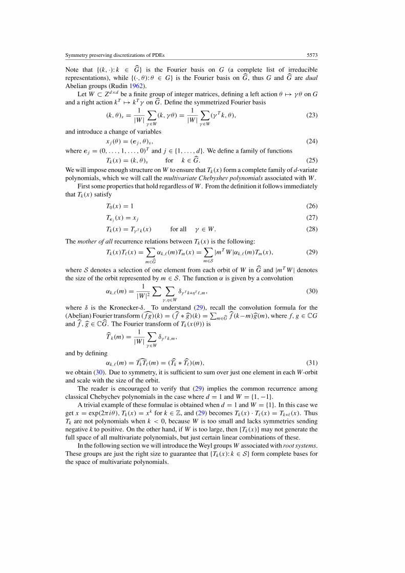
Figure 7. (a) Lebesgue function on deltoid. (b) Lebesgue function on straightened triangle.

Patching deltoids with overlap is an attractive alternative. The deltoid has the remarkableproperty of circumscribing any triangle such that each side of the triangle is tangent to a sideof the deltoid, figure 6(b). It is not difficult to match nodes in two different patches along thenaturally straight lines of the deltoid.

We want to numerically study the quality of interpolation on the deltoid and thestraightened deltoid. Approximation theory on triangles is far less developed than on separabledomains, and very little is known about choice of good interpolation points on triangles.Hesthaven (1998) has studied generalizations of Stieltjes electrostatic characterization ofJacobi–Gauss–Lobatto points from 1D to 2D, and produced interpolation points by numericalcomputations. In Taylor et al (2000), Fekete interpolation points are found by maximizinga Vandermonde determinant in a numerical optimization, see also Bos (1983), Chen andBabuska (1995), Fekete (1923). Fekete triangle points and icosahedral subdivisions of the

5582 H Z Munthe-Kaas

0 50 100 150 200 250 300

0

5

10

15

20

25

30

35

40

HesthavenUniform

Fekete

Chebyshev ∆ pts

No. of nodal pointsLe

besg

ue c

onst

ant

Chebyshev on Deltoid

5 1510 20Polynomial degree

Figure 8. Lebesgue constants for various nodal points on the triangle and deltoid. Bottom curve:points x(�m) on deltoid. All other curves: interpolation on triangle, from top: uniform points;Hesthaven electrostatic points; x(�m) straightened to triangle (37)–(38); Fekete points.

sphere is used for nodal based spectral element discretizations of shallow water equations inGiraldo and Warburton (2005).

The quality of a set of interpolation points I can be measured by the Lebesgue constant,defined as L = ‖I‖∞, where I is the (multivariate) interpolation operator in the given nodes.Slow growth of the Lebesgue constant is necessary for spectral convergence. Uniform pointstypically show exponential growth. Points with the minimal Lebesgue constant are calledLebesgue points, but there are no known algorithm for computing these. It is known that theLebesgue constant for the optimal Lebesgue points grow logarithmically in the number ofpoints. For the 1D Chebyshev–Lobatto points, it is known that the Lebesgue constant growslogarithmically. The proof can be generalized to our points x(�m) ⊂ δ, so probably thesepoints have near optimal interpolation properties. It is not known if the same property holdsfor the interpolation points in the straightened deltoid.

Numerically, we can compute the Lebesgue constant by computing the Lebesgue function

λ(x) =∑i∈I

|�i(x)|,

where �i(x) is the Lagrangian cardinal polynominal at node i. After computing λ(x) on avery fine lattice, we find the Lebesgue constant taking the maximum: L = ‖λ(x)‖∞. Figure 7shows the Lebesgue constants on the deltoid and straightened triangle. In figure 8, we seeLebesgue constants for various choices of interpolation points.

Symmetry preserving discretizations of PDEs 5583

The interpolation points on the deltoid show excellent behaviour. Even when m = 60,yielding 631 nodal points and polynomials of degree 35, the Lebesgue constant is 9.1, and thecondition number of the Chebyshev Vandermonde matrix is just 3.6.

The Lebesgue constant for the nodal points on the straightened triangle are also good.The growth of these seems to be faster than logarithmic, but they are better then the Hesthavenpoints and not much worse than the Fekete points, which requires optimization algorithmsto be found. We believe that the Chebyshev-based nodal points are suitable for constructinghigh-order spectral element bases.

A final remark on triangular interpolation. The nodal-based triangular spectral elementsused in Giraldo and Warburton (2005), Hesthaven (1998) are based on a number of interpolationpoints given as (q+1)(q+2)/2. This corresponds to the number of monomials in the triangular-truncated monomial basis {xrys : r + s � q}. The number of nodal points in �m is insteadgiven as the centred triangular numbers

|�m| = 12m(m/3 + 1) + 1.

The linear space in which we do our interpolation and computation of Lebesgue constants isthe space spanned by the Chebyshev polynomials Tk(x) for k ∈ Sm. In this space, the lowermonomials xrys are linearly independent, while the highest monomials appear only in certainlinear combinations. We cannot see that this fact introduces any practical problems for theconstruction of spectral element bases.

4. Concluding remarks

A recurring theme in this paper has been applications of (finite) symmetry groups in thediscretization and solution of PDEs. Group theory provides us with a unified framework fordeveloping discretizations, fast algorithms and software. For triangle-based spectral elements,we believe that methods based on the non-separable multivariate Chebyshev polynomialstype A2 are very promising because of both the excellent approximation properties of thesepolynomials and the availability of fast transforms and Gaussian quadrature rules. Similarly,we believe that the A3 family and the A2 × A1 families are useful for 3D computation.Furthermore, we hope that a combination of equivariant spectral element discretizations inthe space, and exponential integrators in time will yield competitive algorithms for importantclasses of large scale computational problems.

However, there are still obstacles to overcome in order to make such group-based toolsavailable in the toolbox of computational scientists. One problem is the lack of the literaturefocused on applications of group theory in computations. The other problem is the lackof software. It is our conviction that the group theoretical framework enables us to producegeneral software packages for dealing with discrete versions of Chebyshev polynomials relatedto any Dynkin diagram. These are issues to be addressed in future work.

Acknowledgments

I would like to thank Krister Ahlander for discussions on the topics of the paper, and forsuggesting a number of corrections and improvements of the manuscript.

References

Ahlander K and Munthe-Kaas H 2005 BIT 45Allgower E L, Bohmer K, Georg K and Miranda R 1992 SIAM J. Numer. Anal. 29 534–52

5584 H Z Munthe-Kaas

Allgower E L, Georg K and Miranda R 1993 Lectures in Applied Mathematics vol 29 (Providence, RI: AmericanMathematical Society) ed E L Allgower, K Georg and R Miranda p 23–36

Allgower E L, Georg K, Miranda R and Tausch J 1998 Zeitschrift fur Angewandte Mathematik und Mechanik 78185–201

Beerends R J 1991 Trans.—Am. Math. Soc. 328 779–814Bos L P 1983 J. Approx. Theory 38 43–59Bossavit A 1986 Comput. Methods Appl. Mech. Eng. 56 167–215Chen Q and Babuska I 1995 Comput. Methods. Appl. Mech. Eng. 128 405–17Conway J H and Sloane N J A 1988 Sphere Packing, Lattices and Groups (Berlin: Springer)Douglas C C and Mandel J 1992 Computing 48 73–96Eier R and Lidl R 1982 Math. Ann. 260 93–9Fassler A F and Stiefel E 1992 Group Theoretical Methods and Their Applications (Boston: Birkhauser)Fekete M 1923 Math. Seit. 17 228–49Georg K and Miranda R 1992 Bifurcation and Symmetry ISNM Vol 104 ed E L Allgower, K Bohmer and M Golubisky

(Basel: Birkhauser) p 157–68Giraldo F X and Warburton T 2005 A nodal triangle-based spectral element method for the shallow water equations

on the sphere J. Comput. Phys. 207 129–50Hesthaven J S 1998 SIAM J. Numer. Anal. 35 655–76Hochbruck M and Lubich C 1998 SIAM J. Sci. Comput. 19 1552–74Hoffman M E and Withers W D 1988 Trans.—Am. Math. Soc. 308 91–104Humphreys J E 1970 Introduction to Lie Algebras and Representation Theory (Berlin: Springer)Iserles A, Munthe-Kaas H Z, Nørsett S P and Zanna A 2000 Acta Numerica 9 215–365James G and Liebeck M 2001 Representations and Characters of Groups 2nd edn (Cambridge: Cambridge University

Press) ISBN 052100392XKoornwinder T 1974 Indiag. Math. 36 48–66, 357Krogstad S 2005 J. Comput. Phys. 10 72–88Lidl R 1975 J. Reine Angew. Math. 273 178–98Lomont J S 1959 Applications of Finite Groups (New York: Academic)Munthe-Kaas H 1989 Topics in linear algebra for vector- and parallel computers, PhD thesis NTNU Trondheim,

Norway available at: http://hans.munthe-kaas.noMunthe-Kaas H 1999 Appl. Numer. Math. 29 115–27Munthe-Kaas H 2006 Multivariate Chebyshev polynomials in computations to appearOwren B 2006 Order conditions for commutator-free Lie group methods J. Phys. A: Math. Gen. 39 5585–99Puschel M and Rotteler M 2004 Proc. 11th IEEE DSP WorkshopRudin W 1962 Fourier Analysis on Groups (New York: Wiley)Serre J P 1977 Linear Representations of Finite Groups (Berlin: Springer) ISBN 0387901906Taylor M A, Wingate B A and Vincnent R E 2000 SIAM J. Numer. Anal. 38 1707–20Trønnes A 2005 Symmetries and Generalized Fourier Transforms applied to computing the matrix exponential

Master’s Thesis University of Bergen, Norway