On generalizations of network design problems with degree bounds

Math. Program., Ser. A (2013) 141:479–506DOI 10.1007/s10107-012-0537-8

FULL LENGTH PAPER

On generalizations of network design problemswith degree bounds

Nikhil Bansal · Rohit Khandekar · Jochen Könemann ·Viswanath Nagarajan · Britta Peis

Received: 8 March 2011 / Accepted: 22 March 2012 / Published online: 5 April 2012© Springer and Mathematical Optimization Society 2012

Abstract Iterative rounding and relaxation have arguably become the method ofchoice in dealing with unconstrained and constrained network design problems. Inthis paper we extend the scope of the iterative relaxation method in two directions: (1)by handling more complex degree constraints in the minimum spanning tree problem(namely laminar crossing spanning tree), and (2) by incorporating ‘degree bounds’in other combinatorial optimization problems such as matroid intersection and latticepolyhedra. We give new or improved approximation algorithms, hardness results, andintegrality gaps for these problems. Our main result is a (1, b+O(log n))-approxima-tion algorithm for the minimum crossing spanning tree (MCST) problem with laminardegree constraints. The laminar MCST problem is a natural generalization of the well-studied bounded-degree MST, and is a special case of general crossing spanning tree.

A preliminary version of this paper appeared as [5].

N. BansalEindhoven University of Technology, Eindhoven, The Netherlandse-mail: [email protected]

R. Khandekar · V. Nagarajan (B)IBM T.J. Watson Research Center, Yorktown Heights, NY, USAe-mail: [email protected]

R. Khandekare-mail: [email protected]

J. KönemannUniversity of Waterloo, Waterloo, ON, Canadae-mail: [email protected]

B. PeisTechnische Universität Berlin, Berlin, Germanye-mail: [email protected]

123

480 N. Bansal et al.

We give an additive �(logc m) hardness of approximation for general MCST, evenin the absence of costs (c > 0 is a fixed constant, and m is the number of degreeconstraints). This also leads to a multiplicative �(logc m) hardness of approximationfor the robust k-median problem (Anthony et al. in Math Oper Res 35:79–101, 2010),improving over the previously known factor 2 hardness. We then consider the crossingcontra-polymatroid intersection problem and obtain a (2, 2b+�−1)-approximationalgorithm, where � is the maximum element frequency. This models for example thedegree-bounded spanning-set intersection in two matroids. Finally, we introduce thecrossing lattice polyhedron problem, and obtain a (1, b + 2� − 1) approximationalgorithm under certain condition. This result provides a unified framework and com-mon generalization of various problems studied previously, such as degree boundedmatroids.

Mathematics Subject Classification 90C27 · 68W25

1 Introduction

Iterative rounding and relaxation have arguably become the method of choice in deal-ing with unconstrained and constrained network design problems. Starting with Jain’selegant iterative rounding scheme for the generalized Steiner network problem in [18],an extension of this technique (iterative relaxation) has more recently lead to break-through results in the area of constrained network design, where a number of linearconstraints are added to a classical network design problem. Such constraints arisenaturally in a wide variety of practical applications, and model limitations in process-ing power, bandwidth or budget. The design of powerful techniques to deal with theseproblems is therefore an important goal.

The most widely studied constrained network design problem is the minimum-costdegree-bounded spanning tree problem. In an instance of this problem, we are givenan undirected graph, non-negative costs for the edges, and positive, integral degree-bounds for each of the nodes. The problem is easily seen to be NP-hard, even in theabsence of edge-costs, since finding a spanning tree with maximum degree two isequivalent to finding a Hamiltonian Path. A variety of techniques have been appliedto this problem [9,10,15,20,21,28,29], culminating in Singh and Lau’s breakthroughresult in [33]. They presented an algorithm that computes a spanning tree of at mostoptimum cost whose degree at each vertex v exceeds its bound by at most 1, using theiterative relaxation framework developed in [23,33].

The iterative relaxation technique has been applied to several constrained networkdesign problems: spanning tree [33], survivable network design [23,24], directedgraphs with intersecting and crossing super-modular connectivity [4,23]. It has alsobeen applied to degree bounded versions of matroids and submodular flow [19].

In this paper we further extend the applicability of iterative relaxation, and obtainnew or improved bicriteria approximation results for minimum crossing spanning tree(MCST), crossing contra-polymatroid intersection, and crossing lattice polyhedra. Wealso provide some hardness results and integrality gaps for these problems.

Notation. As is usual, when dealing with an undirected graph G = (V, E), for anyS ⊆ V we let δG(S) := {(u, v) ∈ E | u ∈ S, v �∈ S}. When the graph is clear

123

On generalizations of network design problems with degree bounds 481

from the context, the subscript is dropped. A collection {U1, . . . , Ut } of vertex-sets iscalled laminar if for every pair Ui , U j in this collection, we have Ui ⊆ U j , U j ⊆ Ui ,or Ui ∩ U j = ∅. A (ρ, f (b)) approximation for a minimum cost degree boundedproblem refers to a solution that (1) has cost at most ρ times the optimum that satisfiesthe degree bounds, and (2) satisfies the relaxed degree constraints in which a bound bis replaced with a bound f (b).

1.1 Our results, techniques and paper outline

Laminar MCST. Our main result is for a natural generalization of bounded-degreeMST (called laminar minimum crossing spanning tree or laminar MCST), where weare given an edge-weighted undirected graph with a laminar family L = {Si }mi=1of vertex-sets having bounds {bi }mi=1; and the goal is to compute a spanning tree ofminimum cost that contains at most bi edges from δ(Si ) for each i ∈ [m].

The motivation behind this problem is in designing a network where there is a hier-archy (i.e. laminar family) of service providers that control nodes (i.e. vertices). Thenumber of edges crossing the boundary of any service provider (i.e. its vertex-cut)represents some cost to this provider, and is therefore limited. The laminar MCSTproblem precisely models the question of connecting all nodes in the network whilesatisfying bounds imposed by all the service providers.

From a theoretical viewpoint, cut systems induced by laminar families are wellstudied, and are known to display rich structure. For example, one-way cut-incidencematrices are matrices whose rows are incidence vectors of directed cuts induced by thevertex-sets of a laminar family; It is well known (e.g., see [22]) that such matrices aretotally unimodular. Using the laminar structure of degree-constraints and the iterativerelaxation framework, we obtain the following main result, and present its proof inSect. 2.

Theorem 1 There is a polynomial time (1, b + O(log n)) bicriteria approximationalgorithm for laminar MCST. That is, the cost is no more than the optimum cost andthe degree violation is at most an additive O(log n). This guarantee is relative to thenatural LP relaxation.

This guarantee is substantially stronger than what follows from known results forthe general MCST problem: where the degree bounds could be on arbitrary edge-sub-sets E1, . . . , Em . In particular, for general MCST a (1, b + � − 1) [4,19] is knownwhere � is the maximum number of degree-bounds an edge appears in. However,this guarantee is not useful for laminar MCST as � can be as large as �(n) in thiscase. If a multiplicative factor in the degree violation is allowed, Chekuri et al. [12]recently gave a very elegant

(1, (1+ ε)b + O

( 1ε

log m))

guarantee, which subsumesthe previous best (O(log n), O(log m) b) result [6]. However, these results also can-not be used to obtain a small additive violation, especially if b is large.1 In particular,

1 An approximation algorithm for MCST is said to have additive degree guarantee of β if, given any instance

with bounds b, its solution has degree≤ b+β. In particular, the (1+ε) ·b+O(

1ε log m

)degree guarantee

from [12] does not imply any non-trivial additive guarantee since it has a multiplicative factor ahead of b.

123


both the results [6,12] for general MCST are based on the natural LP relaxation, forwhich there is an integrality gap of b+�(

√n) even without regard to costs and when

m = O(n) [32] (see also Sect. 3.2). Furthermore, combined with the recent hardnessresult of Charikar et al. [8] on discrepancy minimization, it follows that it is NP-hardto achieve an additive o(

√n) guarantee on degree for MCST (we give more details

later). On the other hand, Theorem 1 shows that a purely additive O(log n) guaran-tee on degree (relative to the LP relaxation and even in presence of costs) is indeedachievable for MCST, when the degree-bounds arise from a laminar cut-family.

The algorithm in Theorem 1 is based on iterative relaxation and uses two mainnew ideas. Firstly, we drop a carefully chosen constant fraction of degree-constraintsin each iteration. This is crucial as it can be shown that dropping one constraint ata time as in the usual applications of iterative relaxation can indeed lead to a degreeviolation of �(�). Secondly, the algorithm does not just drop degree constraints, butin some iterations it also generates new degree constraints, by merging existing degreeconstraints.

All previous applications of iterative relaxation to constrained network design treatconnectivity and degree constraints rather asymmetrically. While the structure of theconnectivity constraints of the underlying LP is used crucially (e.g., in the ubiqui-tous uncrossing argument), the handling of degree constraints is remarkably simple.Constraints are dropped one by one, and the final performance of the algorithm isgood only if the number of side constraints is small (e.g., in recent work by Grandoniet al. [16]), or if their structure is simple (e.g., if the ‘frequency’ of each element issmall). In contrast, our algorithm for laminar MCST exploits the structure of degreeconstraints much more carefully.

Hardness results. We obtain the following hardness of approximation for the gen-eral MCST problem (and its matroid counterpart). In particular this rules out anyalgorithm for MCST that has additive constant degree violation, even without regardto costs.

Theorem 2 Unless NP has quasi-polynomial time algorithms, the MCST problemadmits no polynomial time O(logc m) additive approximation for the degree boundsfor some constant c > 0; this holds even when there are no costs.

The proof for this theorem is given in Sect. 3, and uses a two-step reduction fromthe well-known Label Cover problem. First, we show hardness for a uniform matroidinstance. In a second step, we then demonstrate how this implies the result for MCSTclaimed in Theorem 2.

As mentioned above, in very recent work Charikar et al. [8] showed that it isNP-hard to obtain better than O(

√n) additive approximation for discrepancy minimi-

zation. This implies a b+�(√

n) hardness of approximation for MCST, which is muchstronger than Theorem 2. Still our hardness result has some advantages. Theorem 2 hasthe additional property that all degree bounds in its hard instances are unit; whereasthe degree bounds in the hard instances implied by [8] are �(n). This turns out to beuseful in the (seemingly unrelated) context of robust (or min-max) k-median [1]. Inthis problem, there are m different client-sets in a metric and the goal is to open kfacilities that are simultaneously good (in terms of the k-median objective) for all the

123


client-sets. Anthony et al. [1] obtained a logarithmic approximation algorithm for thisproblem, and showed that it is hard to approximate better than factor 2. The follow-ing result shows that the robust k-median problem is indeed harder to approximatethan usual k-median, for which O(1)-approximation algorithms are known [7,3]. Wepresent its proof in Sect. 3.1.

Corollary 3 Robust k-median is�(logc m)-hard to approximate even on uniform met-rics (for some fixed constant c > 0), assuming NP does not have quasi-polynomialtime algorithms.

Degree bounds in more general settings. We consider crossing versions of otherclassic combinatorial optimization problems, namely contra-polymatroid intersectionand lattice polyhedra [17].

A set function g : 2E → Z (on groundset E) is called supermodular (w.r.t. theBoolean lattice (2E ,⊆,∩,∪)) if, for each A, B ⊆ E we have g(A)+ g(B) ≤ g(A ∪B)+g(A∩B). The contra-polymatroid associated with such an integral supermodularfunction g is the polyhedron {x ∈ R

E : x(U ) ≥ g(U ), ∀U ⊆ E, x ≥ 0}. It is well-known (see Equation (44.38) [31]) that this linear system is box totally dual integral;in particular the polytope {x ∈ R

E : x(U ) ≥ g(U ), ∀U ⊆ E, 0 ≤ x ≤ 1} is integral.Moreover, it is also known (Corollary 46.1d in [31]) that the intersection of two contra-polymatroids (given by integral supermodular functions r1, r2 : 2E → Z) is box totallydual integral. Hence {x ∈ R

E : x(U ) ≥ max{r1(U ), r2(U )} ∀U ⊆ E, 0 ≤ x ≤ 1} isan integral polytope. Contra-polymatroid intersection contains, for example, the span-ning-set intersection in two matroids. We study the natural degree bounded version ofthis problem, i.e.

Definition 4 (Minimum crossing contra-polymatroid intersection) Let r1, r2 : 2E →Z be two supermodular functions, cost function c : E → R+ and {Ei }i∈I be a collec-tion of subsets of E with corresponding bounds {bi }i∈I . Then the goal is to minimize:

{cT x∣∣ x(S) ≥ max{r1(S), r2(S)},∀ S ⊆ E;

x(Ei ) ≤ bi , ∀ i ∈ I ; x ∈ {0, 1}E }.

In particular, this definition captures the degree-bounded version of spanning-setintersection in two matroids (e.g., the bipartite edge-cover problem). We note that thisdefinition does not capture alternate notions of matroid intersection, such as intersec-tion of bases in two matroids; hence it does not apply to the degree-bounded arbores-cence problem.2

Let � = maxe∈E |{i ∈ [m] | e ∈ Ei }| be the largest number of sets Ei that anyelement of E belongs to, and refer to it as frequency. The proof of this theorem canbe found in Sect. 4.

Theorem 5 Any optimal basic solution x∗ of the linear relaxation of the minimumcrossing contra-polymatroid intersection problem can be rounded into an integralsolution x̂ such that:

2 In an earlier version of the paper [5], we had incorrectly claimed that our result extends to degree-boundedarborescence.

123


x̂(S) ≥ max{r1(S), r2(S)}, ∀S ⊆ E; x̂(Ei ) ≤ 2bi +�− 1, ∀i ∈ I ;and cT x̂ ≤ 2cT x∗.

The algorithm for this theorem again uses iterative relaxation, and its proof isbased on a ‘fractional token’ counting argument similar to the one used in [4]. Wealso observe that the natural iterative relaxation steps are insufficient to obtain a betterapproximation guarantee.

It can be observed that uncrossing techniques play an essential role when ana-lyzing iterative relaxation algorithms on combinatorial optimization problems where,additionally, some sort of “degree bound constraints” have been added to the linearinequality system. Thus, when looking for some general framework of systems, let’ssay “totally dual integral” (TDI) system, for which iterative relaxation techniqueslead to “good” approximation guarantees for the corresponding crossing problem, thelattice polyhedron model, as introduced by Hoffman and Schwartz [17] seems to be apromising candidate.

Crossing lattice polyhedra. Lattice polyhedra form a unified framework for var-ious discrete optimization problems (like, e.g., contra-polymatroid intersection, orplanar min cut). They are polyhedra of type:

{x ∈ R

E | x(ρ(S)) ≥ r(S), ∀S ∈ F}

where E denotes some arbitrary non-empty finite set, F relates to a collection ofsubsets of E via some mapping ρ : F → 2E , and F induces a lattice-type structure(F ,≤,∧,∨) with some partial order (F ,≤) and binary meet and join operations∧ and∨. It is required that F and ρ satisfy certain submodularity and consecutive properties(which are easily seen to be true for the Boolean lattice with the identity map), andr is supermodular w.r.t. ∧ and ∨. A precise definition is given in Sect. 5, where wealso mention some examples of lattice polyhedra. The key property of lattice poly-hedra is that the uncrossing technique can be applied. Using this uncrossing propertyit is not hard to see that the underlying system is box-TDI [17], and min-max theo-rems for several classical discrete optimization problems find their explanation thisway. The integrality result of Hoffman and Schwartz was just a theoretical existenceresult without algorithmic foundation. Recently, the first combinatorial algorithm wasfound [26]. We refer the reader to [31] for a more comprehensive treatment of thissubject.

Thus, as uncrossing techniques are crucial in almost all iterative relaxationapproaches for optimization problems with degree bounds, we generalize our workeven further and consider crossing lattice polyhedra which arise from lattice poly-hedra by adding “degree-constraints” of the form ai ≤ x(Ei ) ≤ bi for a givencollection {Ei ⊆ E | i ∈ I } and lower and upper bounds a, b ∈ R

I . We showthat the standard LP relaxation for the general crossing lattice polyhedron prob-lem is weak; in Sect. 5.1 we give instances of crossing planar min-cut where theLP-relaxation is feasible, but any integral solution violates some degree-bound by�(√

n). For this reason, we henceforth focus on arestricted class of crossing lattice

123


polyhedra in which the underlying lattice (F ,≤) satisfies the following monotonicityproperty:

S < T �⇒ |ρ(S)| < |ρ(T )| ∀ S, T ∈ F . (*)

We obtain the following theorem whose proof is given in Sect. 5.

Theorem 6 For any instance of the crossing lattice polyhedron problem in which Fsatisfies property (∗), there exists an algorithm that computes an integral solution ofcost at most the optimal, where all rank constraints are satisfied, and each degreebound is violated by at most an additive 2�− 1.

We note that the above property (∗) is satisfied for matroids, and hence Theorem 6matches the previously best-known bound [19] for degree bounded matroids (withboth upper/lower bounds). Also note that property (∗) holds whenever F is orderedby inclusion.

1.2 Related work

As mentioned earlier, the basic bounded-degree MST problem has been extensivelystudied [9,10,15,20,21,28,29,33]. The iterative relaxation technique for degree-con-strained problems was developed in [23,33].

MCST was first introduced by Bilo et al. [6], who presented a randomized-roundingalgorithm that computes a tree of cost O(log n) times the optimum where each degreeconstraint is violated by a multiplicative O(log n) factor and an additive O(log m)

term. Subsequently, Bansal et al. [4] gave an algorithm that attains an optimal costguarantee and an additive � − 1 guarantee on degree; recall that � is the maxi-mum number of degree constraints that an edge lies in. This algorithm used itera-tive relaxation as its main tool. Recently, Chekuri et al. [12] obtained an improved(1, (1+ ε)b + O

( 1ε

log m))

approximation algorithm for MCST, for any ε > 0; thisalgorithm is based on pipage rounding.

The minimum crossing matroid basis problem was introduced in [19], where theauthors used iterative relaxation to obtain (1) (1, b+�−1)-approximation algorithmwhen there are only upper bounds on degree, and (2) (1, b+ 2�− 1)-approximationalgorithm in the presence of both upper and lowed degree-bounds. The [12] result alsoholds in this matroid setting. [19] also considered a degree-bounded version of thesubmodular flow problem and gave a (1, b + 1) approximation guarantee.

The bounded-degree arborescence problem was considered in Lau et al. [23], wherea (2, 2b + 2) approximation guarantee was obtained. Subsequently Bansal et al. [4]designed an algorithm that for any 0 < ε ≤ 1/2, achieves a (1/ε, bv/(1 − ε) + 4)

approximation guarantee. They also showed that this guarantee is the best one canhope for via the natural LP relaxation (for every 0 < ε ≤ 1/2). In the absence ofedge-costs, [4] gave an algorithm that violates degree bounds by at most an additivetwo. Recently Nutov [27] studied the arborescence problem under weighted degreeconstraints, and gave a (2, 5b) approximation algorithm for it.

123


Lattice polyhedra were first investigated by Hoffman and Schwartz [17] and thenatural LP relaxation was shown to be totally dual integral. As stated above, the inte-grality result of Hoffman and Schwartz was not accompanied by an algorithm. Inthe last decades, several algorithms, often of greedy-type, have been established forspecial subclasses of lattice polyhedra. The farthest reaching greedy-type algorithmsfor lattice polyhedra are, most probably, the algorithms in [14] and [13]. However,in all these algorithms, the rank function was required to be monotone increasing onthe underlying lattice, a property which does not hold for, e.g., contra-polymatroidintersection. Recently, the first combinatorial algorithm was established for latticepolyhedra in general [26].

2 Crossing spanning tree with laminar degree bounds

In this section we prove Theorem 1 by presenting an iterative relaxation-based algo-rithm with the stated performance guarantee. During its execution, the algorithmselects and deletes edges, and it modifies the given laminar family of degree bounds.A generic iteration starts with a subset F of edges already picked in the solution,a subset E of undecided edges, i.e., the edges not yet picked or dropped from thesolution, a laminar family L on V , and residual degree bounds b(S) for each S ∈ L.

The laminar family L has a natural forest-like structure with nodes correspondingto each element of L. A node S ∈ L is called the parent of node C ∈ L if S is theinclusion-wise minimal set in L \ {C} that contains C ; and C is called a child of S.Node D ∈ L is called a grandchild of node S ∈ L if S is the parent of D’s parent.A node that has no parent is called root. Nodes S, T ∈ L are siblings if they have thesame parent node; we also define the set of all root nodes to be siblings. The levelof any node S ∈ L is the length of the path in this forest from S to the root of itstree. We also maintain a linear ordering of the children of each L-node. A subsetB ⊆ L is called consecutive if all nodes in B are siblings (with some parent S) andthey appear consecutively in the ordering of S’s children. In any iteration (F, E,L, b),the algorithm solves the following LP relaxation of the residual problem.

min∑

e∈E

cexe (1)

s.t. x(E(V )) = |V | − |F | − 1

x(E(U )) ≤ |U | − |F(U )| − 1 ∀U ⊂ V

x(δE (S)) ≤ b(S) ∀S ∈ Lxe ≥ 0 ∀e ∈ E

For any vertex-subset W ⊆ V and edge-set H , we let H(W ) := {(u, v) ∈ H |u, v ∈ W } denote the edges induced on W ; and δH (W ) := {(u, v) ∈ H | u ∈ W, v �∈W } the set of edges crossing W . The first two sets of constraints are spanning treeconstraints while the third set corresponds to the degree bounds. Let x denote an opti-mal extreme point solution to this LP. By reducing degree bounds b(S), if needed, weassume that x satisfies all degree bounds at equality (the degree bounds may thereforebe fractional-valued). Let α := 24.

123


Fig. 1 Example of local edges

B1

B2

C1

S C4

C3

C2

Definition 7 An edge e ∈ E is said to be local for S ∈ L if e has at least one end-pointin S but is neither in E(C) nor in δ(C)∩ δ(S) for any grandchild C of S. Let local(S)

denote the set of local edges for S. A node S ∈ L is said to be good if |local(S)| ≤ α.

Figure 1 shows a set S, its children B1 and B2, and grand-children C1, . . . , C4;edges in local(S) are drawn solid, non-local ones are shown dashed.

Initially, E is the set of edges in the given graph, F ← ∅,L is the original laminarfamily of vertex sets for which there are degree bounds, and an arbitrary linear order-ing is chosen on the children of each node in L. In a generic iteration (F, E,L, b),the algorithm performs one of the following steps (see also Fig. 2):

1. If xe = 1 for some edge e ∈ E then F ← F ∪ {e}, E ← E \ {e}, and setb(S) ← b(S)− 1 for all S ∈ L with e ∈ δ(S).

2. If xe = 0 for some edge e ∈ E then E ← E \ {e}.3. DropN: Suppose there at least |L|/4 good non-leaf nodes in L. Then either odd-

levels or even-levels contain a set M ⊆ L of |L|/8 good non-leaf nodes. Dropthe degree bounds of all children of M and modify L accordingly. The orderingof siblings also extends naturally.

4. DropL: Suppose there are more than |L|/4 good leaf nodes in L, denoted by N .Then partition N into parts corresponding to siblings in L. For any part {N1, . . . ,

Nk} ⊆ N consisting of ordered (not necessarily contiguous) children of somenode S:

Fig. 2 Examples of the degree constraint modifications DropN and DropL

123


(a) Define Mi = N2i−1 ∪ N2i for all 1 ≤ i ≤ �k/2� (if k is odd Nk is not used).(b) Modify L by removing leaves {N1, . . . , Nk} and adding new leaf-nodes

{M1, . . . , M�k/2�} as children of S (if k is odd Nk is removed). The chil-dren of S in the new laminar family are ordered as follows: each node Mi

takes the position of either N2i−1 or N2i (arbitrarily), and other children ofS are unaffected.

(c) Set the degree bound of each Mi to b(Mi ) = b(N2i−1)+ b(N2i ).

Assuming that one of the above steps applies at each iteration, the algorithm ter-minates when E = ∅ and outputs the final set F as a solution. It is clear that thealgorithm outputs a spanning tree of G. An inductive argument (see e.g. [23]) can beused to show that the LP (1) is feasible at each iteration and c(F)+ zcur ≤ zo wherezo is the original LP value, zcur is the current LP value, and F is the chosen edge-setat the current iteration. Thus the cost of the final solution is at most the initial LPoptimum zo. Next we show that one of the four iterative steps always applies.

Lemma 8 In each iteration, one of the four steps above applies.

Proof Let x∗ be the optimal basic solution of (1), and suppose that the first two stepsdo not apply. Hence, we have 0 < x∗e < 1 for all e ∈ E . The fact that x∗ is a basicsolution together with a standard uncrossing argument (e.g., see [18]) implies that x∗is uniquely defined by

x(E(U )) = |U | − |F(U )| − 1 ∀U ∈ S, and x(δE (S)) = b(S), ∀ S ∈ L′,

where S is a laminar subset of the tight spanning tree constraints, and L′ is a subsetof tight degree constraints; moreover this set of constraints are linearly independentand |E | = |S| + |L′|.

A simple counting argument using extreme-point properties of x∗ yields 2|S| ≤ |E |(see, e.g., [33]); we give a proof below for completeness.

Claim 9 The number |S| of tight linearly independent spanning tree constraints ofx∗ is at most |E |/2.

Proof Recall that E denotes the support of the extreme point solution x∗. Consider anyU ∈ S. Let {Wi } denote the set of U ’s children in S; i.e. the inclusion-wise maximalsets in S \ {U } that are subsets of U . We will show that |E(U ) \ ∪i E(Wi )| ≥ 2; notethat this suffices to prove the claim.

Observe that x∗(E(U ) \⋃

i E(Wi )) = x∗(E(U )) −∑

i x∗(E(Wi )) is an integersince U and {Wi } are tight spanning tree constraints (with integer values). More-over E(U ) \ ⋃

i E(Wi ) �= ∅ since the constraints U and {Wi } are linearly inde-pendent; hence x∗

(E(U ) \⋃

i E(Wi ))

> 0 (recall x∗e > 0 for all e ∈ E). Thuswe have x∗

(E(U ) \⋃

i E(Wi )) ≥ 1. As x∗e < 1 for all e ∈ E , it follows that

|E(U ) \ ∪i E(Wi )| ≥ 2 ��Using this claim and |E | = |S|+|L′|, we obtain |S| ≤ |L′| and |E | ≤ 2|L′| ≤ 2|L|.From the definition of local edges, we get that any edge e = (u, v) is local to at most

the following six sets: the smallest set S1 ∈ L containing u, the smallest set S2 ∈ L

123


containing v, the parents P1 and P2 of S1 and S2 resp., the least-common-ancestor Lof P1 and P2, and the parent of L . Thus

∑S∈L |local(S)| ≤ 6|E |. From the above,

we conclude that∑

S∈L |local(S)| ≤ 12|L|. Thus at least |L|/2 sets S ∈ L must have|local(S)| ≤ α = 24, i.e., must be good. Now either at least |L|/4 of them must benon-leaves or at least |L|/4 of them must be leaves. In the first case, step 3 holds andin the second case, step 4 holds. ��

It remains to bound the violation in the degree constraints, which turns out to berather challenging. We note that this is unlike usual applications of iterative round-ing/relaxation, where the harder part is in showing that one of the iterative stepsapplies.

It is clear that the algorithm reduces the size of L by at least |L|/8 in each DropNor DropL iteration. Since the initial number of degree constraints is at most 2n − 1,we get the following lemma.

Lemma 10 The number of drop iterations (DropN and DropL) is T := O(log n).

Performance guarantee for degree constraints. We begin with some notation.The iterations of the algorithm are broken into periods between successive drop itera-tions: there are exactly T drop-iterations (Lemma 10). In what follows, the t-th dropiteration is called round t . The time t refers to the instant just after round t ; time 0refers to the start of the algorithm. At any time t , consider the following parameters.

• Lt denotes the laminar family of degree constraints.• Et denotes the undecided edge set, i.e., support of the current LP optimal solution.• For any set B of consecutive siblings in Lt , Bnd(B, t) = ∑

N∈B b(N ) equals thesum of the residual degree bounds on nodes of B.

• For any set B of consecutive siblings in Lt , Inc(B, t) equals the number of edgesfrom δEt (∪N∈B N ) included in the final solution.

Recall that b denotes the residual degree bounds at any point in the algorithm. Thefollowing lemma is the main ingredient in bounding the degree violation.

Lemma 11 For any set B of consecutive siblings in Lt (at any time t), Inc(B, t) ≤Bnd(B, t)+ 4α · (T − t).

Observe that this implies the desired bound on each original degree constraint S:using t = 0 and B = {S}, the violation is bounded by an additive 4α · T term.

Proof The proof of this lemma is by induction on T − t . The base case t = T istrivial since the only iterations after this correspond to including 1-edges: hence thereis no violation in any degree bound, i.e. Inc({N }, T ) ≤ b(N ) for all N ∈ LT . Hencefor any B ⊆ L (not necessarily consecutive), Inc(B, T ) ≤ ∑

N∈B Inc({N }, T ) ≤∑N∈B b(N ) = Bnd(B, T ).Now suppose t < T , and assume the lemma for t + 1. Fix a consecutive B ⊆ Lt .

We consider different cases depending on what kind of drop occurs in round t + 1.

DropN round. Here either all nodes in B get dropped or none gets dropped.

123


Case 1: None of B is dropped. Then observe that B is consecutive in Lt+1 as well; sothe inductive hypothesis implies Inc(B, t+1) ≤ Bnd(B, t+1)+4α ·(T−t−1). Sincethe only iterations strictly between round t and round t+1 involve edge-fixing, we haveInc(B, t) ≤ Bnd(B, t)−Bnd(B, t+1)+Inc(B, t+1) ≤ Bnd(B, t)+4α·(T−t−1) ≤Bnd(B, t)+ 4α · (T − t).

Case 2: All of B is dropped. Let C (possibly empty) denote the set of all children(in Lt ) of nodes in B. Note that C consists of consecutive siblings in Lt+1, and induc-tively Inc(C, t+1) ≤ Bnd(C, t+1)+4α ·(T − t−1). Let S ∈ Lt denote the parent ofthe B-nodes; so C are grand-children of S in Lt . Let x ′ denote the optimal LP solutionjust before round t + 1 (when the degree bounds are still given by Lt ), and H = Et+1the support edges of x ′. At that point, we have b(N ) = x ′(δ(N )) for all N ∈ B ∪ C.Also let Bnd′(B, t + 1) := ∑

N∈B b(N ) be the sum of bounds on B-nodes just beforeround t+1. Since S is a good node in round t+1, |Bnd′(B, t+1)−Bnd(C, t+1)| =|∑N∈B b(N ) −∑

M∈C b(M)| = |∑N∈B x ′(δ(N )) −∑M∈C x ′(δ(M))| ≤ 2α. The

last inequality follows since S is good and all edges contributing to that differencelie in local(S); the factor of 2 appears since some edges, e.g., the edges between twochildren or two grandchildren of S, may get counted twice. Note also that the sym-metric difference of δH (∪N∈B N ) and δH (∪M∈C M) is contained in local(S). ThusδH (∪N∈B N ) and δH (∪M∈C M) differ in at most α edges.

Again since all iterations between time t and t + 1 are edge-fixing:

Inc(B, t) ≤ Bnd(B, t)− Bnd′(B, t + 1)+ |δH (∪N∈B N ) \ δH (∪M∈C M)|+Inc(C, t + 1)

≤ Bnd(B, t)− Bnd′(B, t + 1)+ α + Inc(C, t + 1)

≤ Bnd(B, t)− Bnd′(B, t + 1)+ α + Bnd(C, t + 1)+ 4α · (T − t − 1)

≤ Bnd(B, t)−Bnd′(B, t + 1)+α+Bnd′(B, t + 1)+ 2α+ 4α · (T−t−1)

≤ Bnd(B, t)+ 4α · (T − t)

The first inequality above follows from simple counting; the second follows sinceδH (∪N∈B N ) and δH (∪M∈C M) differ in at most α edges; the third is the inductionhypothesis, and the fourth is Bnd(C, t + 1) ≤ Bnd′(B, t + 1)+ 2α (as shown above).

DropL round. In this case, let S be the parent of B-nodes in Lt , and N ={N1, · · · , Np} be all the ordered children of S, of which B is a subsequence (since itis consecutive). Suppose indices 1 ≤ π(1) < π(2) < · · · < π(k) ≤ p correspond togood leaf-nodes in N . Then for each 1 ≤ i ≤ �k/2�, nodes Nπ(2i−1) and Nπ(2i) aremerged in this round. Let {π(i) | e ≤ i ≤ f } (possibly empty) denote the indices ofgood leaf-nodes in B. Then it is clear that the only nodes of B that may be mergedwith nodes outside B are Nπ(e) and Nπ( f ); all other B-nodes are either not merged ormerged with another B-node. Let C be the inclusion-wise minimal set of children ofS in Lt+1 that is consecutive and contains:

• all nodes of B \ {Nπ(i)}ki=1, and• every new leaf node resulting from merging two good leaf nodes of B.

We remark that C may contain more nodes than these two types, but it is chosen tobe the minimal consecutive set containing all the above nodes. See also Fig. 3 for some

123


(a) (b)

Fig. 3 Deriving set C (shown dotted) from B (shown dashed) in DropL round. a Example has p = 11siblings and k = 6 good leaves, b Example has p = 9 siblings and k = 5 good leaves

examples. Note that ∪M∈C M consists of some subset of B and at most two good leaf-nodes fromN \B. These two extra nodes (if any) are Nπ(e−1) and Nπ( f+1), which mightbe merged with Nπ(e) and Nπ( f ) respectively. Again let Bnd′(B, t+1) :=∑

N∈B b(N )

denote the sum of bounds on B just before drop round t + 1, when degree constraintsare Lt . Let H = Et+1 be the undecided edges in round t + 1. By the definition ofbounds on merged leaves, we have Bnd(C, t + 1) ≤ Bnd′(B, t + 1)+ 2α. The term2α is present due to the (possibly) two extra good leaf-nodes described above.

Claim 12 We have |δH (∪N∈B N ) \ δH (∪M∈C M)| ≤ 2α.

Proof We say that N ∈ N is represented in C if either N ∈ C or N is contained insome node of C. Let D consist of (i) nodes of B that are not represented in C, and(ii) nodes of N \ B that are represented in C. Observe that by definition of C, theset D ⊆ {Nπ(e−1), Nπ(e), Nπ( f ), Nπ( f+1)}; in fact it can be easily seen that |D| ≤ 2.Moreover D consists of only good leaf nodes. (See Fig. 3 for an example). Thus, wehave | ∪L∈D δH (L)| ≤ 2α. Now note that the edges in δH (∪N∈B N ) \ δH (∪M∈C M)

must be in ∪L∈DδH (L). This completes the proof. ��

As in the previous case, we have:

Inc(B, t) ≤ Bnd(B, t)− Bnd′(B, t + 1)+ |δH (∪N∈B N ) \ δH (∪M∈C M)|+Inc(C, t + 1)

≤ Bnd(B, t)− Bnd′(B, t + 1)+ 2α + Inc(C, t + 1)

≤ Bnd(B, t)− Bnd′(B, t + 1)+ 2α + Bnd(C, t + 1)+ 4α · (T − t − 1)

≤ Bnd(B, t)−Bnd′(B, t + 1)+2α+Bnd′(B, t + 1)+2α+4α · (T−t−1)

= Bnd(B, t)+ 4α · (T − t)

The first inequality follows from simple counting; the second uses Claim 12, thethird is the induction hypothesis (since C is consecutive), and the fourth is Bnd(C, t+1)

≤ Bnd′(B, t + 1)+ 2α (from above).This completes the proof of the inductive step and hence Lemma 11. ��

123


3 Hardness results

In this section we prove Theorem 2; i.e. unless NP has quasi-polynomial time algo-rithms, there is no polynomial time O(logc m) additive approximation algorithm fordegree bounds for the MCST problem, where c > 0 is some universal constant. Thisresult also holds in the absence of edge-costs. We note that this hardness result onlyholds for the general MCST problem, and not the laminar MCST addressed earlier.The first step to proving this result is a hardness for the more general minimum cross-ing matroid basis problem: given a matroid M on a ground set V of elements, a costfunction c : V → R+, and degree bounds specified by pairs {(Ei , bi )}mi=1 (where eachEi ⊆ V and bi ∈ N), find a minimum cost basis I in M such that |I ∩ Ei | ≤ bi forall i ∈ [m].Theorem 13 Unless NP has quasi-polynomial time algorithms, the unweighted min-imum crossing matroid basis problem admits no polynomial time O(logc m) additiveapproximation algorithm for the degree bounds for some fixed constant c > 0.

Proof We reduce from the label cover problem [2]. The input is a bipartite graphH = (V1, V2, F) with label set and constraints Cu,v ⊆ × (consisting ofordered pairs of labels) for all (u, v) ∈ F . The goal is to compute an assignmentf : V1

⋃V2 → such that the maximum number of constraints are satisfied, where

constraint Cu,v is said to be satisfied if and only if 〈 f (u), f (v)〉 ∈ Cu,v . The followingresult is well known.

Theorem 14 ([30]) There exists a universal constant γ > 1 such that for every k ∈ N,there is a reduction from any SAT instance (having size N) to a label cover instance〈H = (V1, V2, F), , {Cu,v}(u,v)∈F }〉 with |H |, |F | = N�(k) and || = 2�(k) suchthat:

• If the SAT instance is satisfiable, the label cover instance has optimal value |F |.• If the SAT instance is not satisfiable, the label cover instance has optimal value

< |F |/γ k .

For our reduction, it is convenient to reduce to the following (equivalent) version ofthe label cover problem. We construct a graph G = (U, E) where U = (V1

⋃V2)×

and

E = {((v1, a), (v2, b)) : (v1, v2) ∈ F and 〈a, b〉 ∈ Cv1,v2}.

Observe that the vertex set U is clearly partitioned into n = |V1| + |V2| partsU1, . . . , Un each having size ||, and all edges in E are between distinct parts. Wedenote this instance by 〈G = (U, E), ||, |F |〉. The goal here is to pick one ver-tex from each part {Ui }ni=1 so as to maximize the number of induced edges. Clearlythis is equivalent to the above definition of the label cover problem. Note also that|E | ≤ ||2 · |F |.

Restating Theorem 14 yields: there is a constant γ > 1 such that for every k ∈ N,there is a reduction from SAT instances (of size N ) to “label cover” instances 〈G =(U, E), q, t〉 such that:

123


• If the SAT instance is satisfiable, the label cover instance has optimal value t .• If the SAT instance is not satisfiable, the label cover instance has optimal value

< t/γ k .• |G| = N�(k), number of labels q = 2�(k), |E | ≤ t2, and the reduction runs in

time N O(k).

We consider a uniform matroid M with rank t on ground set E (recall that anysubset of t edges is a basis in a uniform matroid). We now construct a crossing matroidbasis instance I on M. There is a set of degree bounds corresponding to each parti ∈ [n]: for every collection C of edges incident to vertices in Ui such that no twoedges in C are incident to the same vertex in Ui , there is a degree bound in I requiringat most one element to be chosen from C . Note that the number of degree bounds mis at most |E |q ≤ N O(k 2k ). The following claim links the SAT and crossing matroidinstances.

Claim 15 [Yes instance] If the SAT instance is satisfiable, there is a basis (i.e. subsetB ⊆ E with |B| = t) satisfying all degree bounds.[No instance] If the SAT instance is unsatisfiable, every subset B ′ ⊆ E with |B ′| ≥ t/2violates some degree bound by an additive ρ = γ k/2/

√2.

Proof Observe that if the original SAT instance is satisfiable, then the matroid Mcontains a basis obeying all the degree bounds: namely the t edges T ∗ ⊆ E induced inthe optimal solution to the label cover instance. This is because if we consider any Ui ,then all the T ∗-edges having a vertex in Ui as their endpoint, have the same endpoint.Thus, for any degree bound corresponding to collection C (as defined above), at mostone T ∗-edge can lie in C .

Now consider the case that the SAT instance is unsatisfiable. Let B ′ ⊆ E be anysubset with |B ′| ≥ t/2. We claim that B ′ contains at least ρ = γ k/2/

√2 edges from

some degree-constrained set of edges. Suppose (for a contradiction) that |B ′ ∩C | < ρ

for each degree constraint C . This means in particular that each part {Ui }ni=1 con-tains fewer than ρ vertices that are incident to edges of B ′. For each part i ∈ [n], letWi ⊆ Ui denote the vertices incident to edges of B ′; note that |Wi | < ρ. Considerthe label cover solution obtained as follows. For each i ∈ [n], choose one vertex fromWi independently and uniformly at random. Clearly, the expected number of edges inthe resulting induced subgraph is at least |B ′|/ρ2 ≥ t

2ρ2 = t/γ k . This contradicts the

fact that the value of label cover instance is strictly less than t/γ k . ��The steps described in the above reduction can be done in time polynomial in m and

|G|. Also, instead of randomly choosing vertices from the sets Wi , we can use condi-tional expectations to derive a deterministic algorithm that recovers at least t/ρ2 edges.Setting k = �(log log N ) (recall that N is the size of the original SAT instance), weobtain an instance of bounded-degree matroid basis of size≈ m ≤ N O(k 2k ) ≤ N loga N

for some constant a. Also ρ ≥ γ k/2/2 ≥ 2�(k) ≥ logb N , where b > 0 is a constant.Note that log m ≤ loga+1 N , which implies ρ ≥ logc m for c = b

a+1 > 0, a constant.Thus it follows that for this constant c > 0 the bounded-degree matroid basis problemhas no polynomial time O(logc m) additive approximation algorithm for the degreebounds, unless NP has quasi-polynomial time algorithms. ��

We now prove Theorem 2.

123


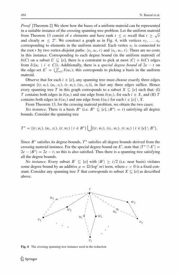
Proof [Theorem 2] We show how the bases of a uniform matroid can be representedin a suitable instance of the crossing spanning tree problem. Let the uniform matroidfrom Theorem 13 consist of e elements and have rank t ≤ e; recall that t ≥ √

eand clearly m ≤ 2e. We construct a graph as in Fig. 4, with vertices v1, . . . , ve

corresponding to elements in the uniform matroid. Each vertex vi is connected tothe root r by two vertex-disjoint paths: 〈vi , ui , r〉 and 〈vi , wi , r〉. There are no costsin this instance. Corresponding to each degree bound (in the uniform matroid) ofb(C) on a subset C ⊆ [e], there is a constraint to pick at most |C | + b(C) edgesfrom δ({ui | i ∈ C}). Additionally, there is a special degree bound of 2e − t onthe edge-set E ′ = ⋃e

i=1 δ(wi ); this corresponds to picking a basis in the uniformmatroid.

Observe that for each i ∈ [e], any spanning tree must choose exactly three edgesamongst {(r, ui ), (ui , vi ), (r, wi ), (wi , vi )}, in fact any three edges suffice. Henceevery spanning tree T in this graph corresponds to a subset X ⊆ [e] such that: (I)T contains both edges in δ(ui ) and one edge from δ(wi ), for each i ∈ X , and (II) Tcontains both edges in δ(wi ) and one edge from δ(ui ) for each i ∈ [e] \ X .

From Theorem 13, for the crossing matroid problem, we obtain the two cases:Yes instance. There is a basis B∗ (i.e. B∗ ⊆ [e], |B∗| = t) satisfying all degree

bounds. Consider the spanning tree

T ∗ = {(r, ui ), (ui , vi ), (r, wi ) | i ∈ B∗}⋃{(r, wi ), (vi , wi ), (r, ui ) | i ∈ [e] \ B∗}.

Since B∗ satisfies its degree-bounds, T ∗ satisfies all degree bounds derived from thecrossing matroid instance. For the special degree bound on E ′, note that |T ∗ ∩ E ′| =2e − |B∗| = 2e − t ; so this is also satisfied. Thus there is a spanning tree satisfyingall the degree bounds.

No instance. Every subset B ′ ⊆ [e] with |B ′| ≥ t/2 (i.e. near basis) violatessome degree bound by an additive ρ = �(logc m) term, where c > 0 is a fixed con-stant. Consider any spanning tree T that corresponds to subset X ⊆ [e] as describedabove.

Fig. 4 The crossing spanning tree instance used in the reduction

123


1. Suppose that |X | ≤ t/2; then we have |T ∩ E ′| = 2e− |X | ≥ 2e− t + t2 , i.e. the

special degree bound is violated by t/2 ≥ �(√

e) = �(log1/2 m).2. Now suppose that |X | ≥ t/2. Then by the guarantee on the no-instance, T violates

some degree-bound derived from the crossing matroid instance by additive ρ.

Thus in either case, every spanning tree violates some degree bound by additive ρ =�(logc m).

By Theorem 13, it is hard to distinguish the above cases and we obtain the corre-sponding hardness result for crossing spanning tree, as claimed in Theorem 2. ��

3.1 Hardness for robust k-median

Another interesting consequence of Theorem 13 is for the robust k-median prob-lem [1]. Here we are given a metric (V, d), m client-sets {Si ⊆ V }mi=1, and bound k;the goal is to find a set F ⊆ V of k facilities such that the worst-case connection cost(over all client-sets) is minimized, i.e.

minF⊆V,|F |=k

mmaxi=1

∑

v∈Si

d(v, F).

Above d(v, F) denotes the shortest distance from v to any vertex in F . Anthonyet al. [1] gave an O(log m+ log k)-approximation algorithm for robust k-median, andshowed that it is hard to approximate better than factor two. At first sight this problemmay seem unrelated to crossing matroid basis. However using Theorem 13, we obtainthe poly-logarithmic hardness result stated in Corollary 3.

Proof Recall that in a uniform metric, the distance between every pair of vertices isone. In this case the robust k-median problem can be rephrased as:

minF⊆V,|F |=k

mmaxi=1

|Si \ F |, where {Si ⊆ V }mi=1 are the client-sets.

The hard instances of crossing matroid basis in Theorem 13 are in fact for uniformmatroids where every degree upper-bound equals one. i.e. there is a ground-set V ,degree bounds given by {Ei ⊆ V }mi=1, and rank t ; the goal is to find (if possible)a subset I ⊆ V with |I | = t such that |I ⋂

Ei | ≤ 1 for all i ∈ [m]. Theorem 13showed that it is hard to distinguish the following cases: (Yes-case) there is someI ⊆ V with |I | = t and maxi∈[m] |I ∩ Ei | ≤ 1; and (No-case) for every I ⊆ V with|I | = t, maxi∈[m] |I ∩ Ei | ≥ ρ := �(logc m).

These hard instances naturally correspond to the robust k-median problem on uni-form metric V , client-sets {Ei ⊆ V }mi=1, and bound k = |V | − t . It is clear that therobust k-median objective is at most one in the Yes-case, and at least ρ in the No-case.Thus we obtain a multiplicative ρ hardness of approximation for robust k-median onuniform metrics. This proves Corollary 3. ��

123


3.2 Integrality gap for general MCST

We now present the b +�(√

n) integrality gap instance for MCST. While such gapsinstances are easy to obtain if one allows m to be super-polynomially large (for exam-ple, by setting a degree bound for each subset of edges), the nice property of theexample here is that m is quite small, in fact m = O(n). This result is due to MohitSingh [32], we thank him for letting us present the example here.

The graph is the same as the one used for the hardness result. The vertex-set is{r}⋃{vi , ui , wi }ei=1, so n = 3e+ 1. The edges are {(r, ui ) | i ∈ [e]} ∪ {(vi , ui ) | i ∈[e]} and {(r, wi ) | i ∈ [e]} ∪ {(vi , wi ) | i ∈ [e]}. See also Fig. 4. There are no costs inthis instance.

The ‘degree bounds’ for the MCST instance are derived from the lower boundfor the discrepancy problem [11]. From discrepancy theory there exists a collection{S j ⊆ [e]}ej=1 of subsets such that,

emaxj=1

∣∣|X ∩ S j | − |X ∩ S j |∣∣ ≥ ρ, for every X ⊆ [e].

Above X = [e]\X as usual, and ρ = �(√

e) = �(√

n). In other words, for every wayof partitioning [e] into two sets, there is some set S j such that the partition inducedon S j has a large imbalance. There are m = 2e degree bounds, defined as follows.For each j ∈ [e] there is a bound of |S j | + �|S j |/2� on each of the edge-sets U j =∪i∈S j δ(ui ) = {(r, ui ), (ui , vi )}i∈S j , and W j = ∪i∈S j δ(wi ) = {(r, wi ), (wi , vi )}i∈S j .

Consider the fractional solution to the natural LP relaxation that sets each edge tovalue 3/4. It is easily seen that it is indeed a fractional spanning tree and satisfies allthe degree bounds.

On the other hand, we claim that any integer solution must violate some degreebound by additive ρ

2 − 1. Note that every spanning tree T in this graph correspondsto a subset X ⊆ [e] such that: (I) T contains both edges in δ(ui ) and one edge fromδ(wi ), for each i ∈ X , and (II) T contains both edges in δ(wi ) and one edge fromδ(ui ) for each i ∈ X . The number of edges used by tree T in the degree-bounds (foreach j ∈ [e]) are:

• |T ∩U j | = 2 |X ∩ S j | + |X ∩ S j | = |S j | + |X ∩ S j |, and• |T ∩W j | = |X ∩ S j | + 2 |X ∩ S j | = |S j | + |X ∩ S j |.

From the discrepancy instance, it follows that maxej=1

∣∣|X ∩ S j | − |X ∩ S j |∣∣ ≥ ρ;

let k be the index achieving this maximum. Then we have:

max{|T ∩Uk |, |T ∩Wk |} = |Sk | +max{|X ∩ Sk |, |X ∩ Sk |} ≥ |Sk | + |Sk |2+ ρ

2.

Thus the degree-bound for either Uk or Wk is violated by additive ρ2 − 1.

Remark The above construction is essentially a reduction from discrepancy minimi-zation to MCST. Combined with the hardness result in [8] this implies that, unlessP = N P , MCST admits no o(

√n) additive approximation in degree when the num-

ber of degree bounds m = O(n). We note that degree bounds in this instance have

123


large values, i.e. �(n). On the other hand, all degree bounds in Theorem 13 have unitvalues– this was crucial in proving the hardness for robust k-median.

4 Minimum crossing contra-polymatroid intersection

In this section we consider the crossing contra-polymatroid intersection problem (seeDefinition 4) and prove Theorem 5. The algorithm (given as Algorithm 1) for thisproblem is based on iteratively relaxing the following natural LP relaxation.

min∑

e∈E ′ce · xe

x(S ∩ E ′) ≥ r1(S)− |F ∩ S| ∀S ⊆ E

x(S ∩ E ′) ≥ r2(S)− |F ∩ S| ∀S ⊆ E

x(Ei ∩ E ′) ≤ b′i ∀i ∈ W

0 ≤ xe ≤ 1 ∀e ∈ E ′.

At a generic iteration, E ′ ⊆ E denotes the set of unfixed elements, F ⊆ E the setof chosen elements (recall that E denotes the groundset of the instance), W ⊆ Ithe set of remaining degree bounds, and b′i (for each i ∈ W ) the residual degree-bound in the i th constraint. Observe that this LP can indeed be solved in polynomialtime by the Ellipsoid algorithm: the separation oracle for the first two sets of con-straints involve submodular function minimization for the two functions gi (S) =x(S∩ E ′)+|S∩ F |− ri (S) (with i = 1, 2). The resulting fractional solution can thenbe converted to an extreme point solution of no larger cost, as described in Jain [18].

Algorithm 1 Algorithm for minimum crossing contra-polymatroid intersection.1: Initially, set E ′ = E, F = ∅, W = I, b′i = bi , for all i ∈ I2: while E ′ �= ∅ do3: Compute an optimal extreme point solution x∗ of the LP(E ′, F, W );4: for all e ∈ E ′ with x∗(e) = 0 do5: E ′ ← E ′ \ {e}6: end for7: for all e ∈ E ′ with x∗(e) ≥ 1

2 do8: F ← F ∪ {e}; E ′ ← E ′ \ {e}9: b′i ← b′i − x∗(e), for all i ∈ W with e ∈ Ei10: end for11: for all i ∈ W with |Ei ∩ E ′| ≤ �2b′i � +�− 1 do12: W ← W \ {i}13: end for14: end while15: Return the incidence vector of F ;

Note that this algorithm rounds variables of value x∗(e) ≥ 12 to 1, and hence we

loose a factor of two in the cost and in the degree bounds. Theorem 5 follows as a

123


consequence if we can show that in each iteration, either some variable can be rounded,or some constraint can be dropped.

Lemma 16 If x∗ ∈ RE ′ is an optimal extreme point solution to the above LP for

crossing contra-polymatroid intersection, with 0 < x∗(e) < 12 for all e ∈ E ′, then

there exists i ∈ W such that

|Ei ∩ E ′| ≤ �2b′i� +�− 1

Proof Let T ′i = {χ(E ′ ∩ S)|x∗(S ∩ E ′) = r1(S) − |S ∩ F |, S ⊆ E} for i = 1, 2denote the tight sets from the first two constraints of the LP respectively. Let B′ ={χ(E ′ ∩ Ei )|x∗(Ei ∩ E ′) = b′i , i ∈ W } denote the tight degree constraints. Since x∗is an extreme point solution (and 0 < x∗ < 1), there exist linearly independent tightsets T1 ⊆ T ′1 , T2 ⊆ T ′2 and B ⊆ B′ such that |E ′| = |T1| + |T2| + |B|.

Since x∗ is modular and ri (S)− |S ∩ F | (for i = 1, 2) are supermodular on 2E , itcan be assumed (using uncrossing arguments, see eg. Chapter 44 in [31]) that each of(T1,⊆) and (T2,⊆) forms a chain.3 The following claim goes back to a similar resultfor spanning trees as stated in [4].

Claim 17 For each i = 1, 2, we have |Ti | ≤ x∗(E ′); additionally if |Ti | = x∗(E ′)then E ′ ∈ Ti .

Proof We prove the claim for i = 1. Let T1 = {S1 ⊂ . . . ⊂ Sk} where Sk ⊆ E ′. LetS0 = ∅ and consider an arbitrary pair of subsequent chain elements S j ⊂ S j+1, for anyj ∈ {0, 1, . . . , k − 1}. Since x∗e > 0 for all e ∈ E ′ it follows that x∗(S j+1 \ S j ) > 0.Hence, by the integrality of r1(S)− |S ∩ F | and tight constraints S j and S j+1,

x∗(S j+1\S j ) = x∗(S j+1)−x∗(S j )=r1(S j+1)−|S j+1 ∩ F |−r1(S j )+|S j ∩ F | ≥1.

Summing over i = 0, . . . , k − 1 we therefore obtain the inequality:

x∗(E ′) ≥ x∗(Sk) =k−1∑

j=0

x∗(S j+1 \ S j ) ≥ k = |T1|,

with equality only if E ′ = Sk . ��We now proceed with the proof of Lemma 16. Suppose (for a contradiction) that for

all i ∈ W, |Ei∩E ′| ≥ �2b′i�+�. For each i ∈ W , define Spi :=∑

e∈E ′∩Ei(1−2x∗e ) =

|E ′∩Ei |−2x∗(E ′∩Ei ). Then we have Spi ≥ |E ′∩Ei |−2b′i ≥ |E ′∩Ei |−�2b′i� ≥ �.Hence

∑i∈W Spi ≥ � · |W |.

For each e ∈ E ′, let re := |{i ∈ W : e ∈ Ei }| ≤ � the maximum elementfrequency. Note also that 0 < 1− 2x∗e < 1 for each e ∈ E ′. Now,

∑

i∈W

Spi =∑

e∈E ′re ·

(1− 2x∗e

) ≤ � ·∑

e∈E ′

(1− 2x∗e

)

= � · (|E ′| − 2 · x∗(E ′)) ≤ � · (|E ′| − |T1| − |T2|

)

3 A family (L,⊆) is a chain if and only if for every X, Y ∈ L, either X ⊆ Y or Y ⊆ X .

123


The last inequality uses Claim 17. Note that equality holds above only if E ′ ∈ T1∩T2(by Claim 17), which would contradict the linear independence of T1 and T2. Thus wehave:

∑

i∈W

Spi < � · (|E ′| − |T1| − |T2|) = � · |B| ≤ � · |W |.

However this contradicts the assumption |E ′ ∩ Ei | ≥ �2b′i� +� for all i ∈ W . ��Proof [Theorem 5] Lemma 16 implies that an improvement is possible in each iter-ation of Algorithm 1. Note also that restricting the current LP solution (to E ′) yieldsa feasible solution to the residual LP in the next iteration. Since we only round ele-ments that the LP sets to value at least half, the cost guarantee is immediate. Considerany degree bound i ∈ I ; let b′i denote its residual bound when it is dropped, and F ′(resp. E ′) the set of chosen (resp. unfixed) elements at that iteration. Again, round-ing elements of fractional value at least half implies |Ei ∩ F ′| ≤ �2bi − 2b′i� =2bi −�2b′i� since bi is integer. Furthermore, the number of Ei -elements in the supportof the basic solution at the iteration (i.e., E ′) when constraint i is dropped is at most�2b′i�+�−1. Thus the number of Ei -elements chosen in the final solution is at most|Ei ∩ F ′| + |Ei ∩ E ′| ≤ 2bi − �2b′i� + �2b′i� +�− 1 = 2 · bi +�− 1. ��

Tight example. We note that the natural iterative relaxation steps (used above) areinsufficient to obtain a better approximation guarantee. Consider the special case ofthe crossing bipartite edge cover problem. The instance consists of graph G which isa 4n-length cycle, with its edges partitioned into two perfect matchings E1 and E2.There is a degree-bound of n on each of E1 and E2; so � = 1. Consider the frac-tional solution to the LP-relaxation that assigns value of 1

2 to all edges. It is indeed afractional edge-cover since each vertex is covered to extent one. The degree-boundsare clearly satisfied. It is also an extreme point: note that this is the unique fractionalsolution minimizing the all-ones cost vector. For this extreme point solution, the larg-est edge-value is 1

2 , and the support-size (i.e. 2n) of its degree-constraints is twicetheir bound (i.e. n). Thus the iterative relaxation must either pick a half-edge or dropa degree-constraint that is potentially violated by factor two.

5 Minimum crossing lattice polyhedra

Before formally defining the lattice polyhedron problem, we need to introduce someterminology. We use notation similar to [14]. The groundset of the problem is denotedby E . Let (F ,≤) be a partially ordered set with F �= ∅. We consider a lattice-typestructure (F ,≤,∧,∨), where the two commutative binary operations, meet ∧ andjoin ∨, are defined on all pairs A, B ∈ F , such that A ∧ B ≤ A, B ≤ A ∨ B.

Note that our definition is more general than the usual definition of a lattice, sincethe join A ∨ B is not required to be the least common upper bound of A and B. Inthe lattice polyhedron model, we are given a supermodular function r : F → Z+ on(F ,≤,∧,∨), i.e. r satisfies

r(A)+ r(B) ≤ r(A ∧ B)+ r(A ∨ B), for all A, B ∈ F .

123


Throughout this paper, we call r the rank function of the lattice polyhedron. Finally,there is a set-valued function ρ : F → 2E relating the lattice F to the groundset E ,so that F and ρ satisfy the following two properties:

1. Consecutive property: If A ≤ B ≤ C then ρ(A) ∩ ρ(C) ⊆ ρ(B),2. Submodularity: For all A, B ∈ F , ρ(A ∨ B) ∪ ρ(A ∧ B) ⊆ ρ(A) ∪ ρ(B),

Given a ground set E , a lattice F , a mapping ρ : F → 2E , so that the consecutiveand submodularity property are satisfied, and a supermodular function r : F → Z+,the polyhedron {x ∈ R

E | ∑e∈ρ(S) xe ≥ r(S), ∀S ∈ F} is a lattice polyhedron.

Hoffman and Schwartz [17] showed that the underlying linear inequality system isbox-TDI.

Definition 18 (Minimum crossing lattice polyhedron) Given a lattice polyhedron〈E, (F ,≤), r, ρ, c〉, a cost function c : E → R+, and lower/upper bounds {ai }i∈I

and {bi }i∈I on a collection {Ei ⊆ E}i∈I , the goal is to minimize:

⎧⎨

⎩cT · x |

∑

e∈ρ(S)

xe ≥ r(S), ∀S ∈ F; ai ≤ x(Ei ) ≤ bi , ∀i ∈ I ; x ∈ {0, 1}E⎫⎬

⎭.

As mentioned earlier, several discrete optimization problems fit into the latticepolyhedron model (see e.g. [31]). We give some examples below.

Example 1 Crossing (contra-) polymatroids. Consider the case where F = 2E , ρ isthe identity map, and the partial order in F is the canonical one that is induced by setinclusion. If r is supermodular on the Boolean lattice (2E ,⊆,∩,∪), then P(r) = {x ∈R

E | ∑e∈S xe ≥ r(S), ∀S ⊆ E} is a (contra-)polymatroid in the sense of Edmonds.For any integral cost function c ∈ Z

E+, the polymatroid greedy algorithm efficientlyfinds an integral vector in P(r) of minimal cost. The crossing contra-polymatroidproblem now searches for the minimum cost vector in P(r) satisfying certain degreebounds.

Example 2 Crossing contra-polymatroid intersection. Consider the case of two poly-matroids P(r1) and P(r2), where the two supermodular functions r1 and r2 are definedon the same ground set E . The contra-polymatroid intersection problem, i.e., the prob-lem to find a vector of minimal cost in the intersection of P(r1) and P(r2), can bemodeled as a lattice polyhedron problem via the following reduction: let F := {S′ :S ⊆ E}⋃{S′′ : S ⊆ E} with ρ(S′) = ρ(S′′) = S for each subset S ⊆ E . The partialorder is:

S′ ≤ T ′′, ∀ S, T ⊆ E and S′ ≤ T ′ and S′′ ≥ T ′′; ∀ S ⊆ T ⊆ E .

The meet (∧) and join (∨) operators are defined to be the greatest common lowerbound and least common upper bound, respectively. This is easily seen to satisfy theconsecutivity and submodularity properties. The rank function r for the lattice poly-hedron has r(S′) = r1(S) and r(S′′) = r2(S), for all S ⊆ E , which is supermodularon F . The crossing contra-polymatroid intersection problem asks for the best vectorin the intersection of P(r1) and P(r2) satisfying degree bounds.

123


Example 3 Crossing s, t-planar min cut. Let G = (V, E) be a (directed or undirected)graph with s, t ∈ V , and capacities c : E → Z+ on the edges. Furthermore, let theelements of F correspond to s-t paths in G (i.e., ρ maps each element of F to the edge-set of that s, t-path). The crossing min-cut problem now asks for an edge set C ⊆ Eof minimal capacity so that C forms an s, t-cut in G, and C satisfies certain degreebounds. For the classical min-cut (or dual max-flow) problem, the rank function is theconstant all-ones function, i.e., an edge set forms a s, t-cut if each of the s, t-paths inF is hit at least once. We restrict to the special case where G is s, t-plane, i.e., whereG is given in a planar embedding with s and t on the outer boundary. We consider thepartial order which sets for any pair of s, t-paths P, Q,

P ≤ Q ⇐⇒ P “below” Q in the planar representation.

Again, the meet (∧) and join (∨) are defined to be the greatest common lower boundand least common upper bound respectively. For s, t-plane graphs, this poset inducesa lattice satisfying the consecutive and submodularity properties [25]. Moreover, theall-ones rank function is certainly supermodular. Thus, the crossing s, t-planar min-cutproblem, which involves finding a minimum cost s, t-cut in G that obeys the degreebounds, fits into the model of crossing lattice polyhedra.

5.1 Integrality gap for general crossing lattice polyhedra

We first show that there is a bad integrality gap for crossing lattice polyhedra. Considerthe s, t-planar min-cut instance on graph G = (V, E) in Fig. 5 with vertices s, t ∈ Vas shown. Define edge-sets Ei := {(vi−1, ui, j )}kj=1

⋃{(vi , ui, j )}kj=1 for each i ∈ [k];here we set v0 = s and vk = t . There are only degree upper-bounds in this instance,namely a bound of one on each {Ei }ki=1. Note also that � = 1 in this instance, andthat the size of the ground-set is n = |E | = �(k2).

Consider the LP solution that sets xe = 12k for every edge e ∈ E . It is clearly

feasible for the rank constraints (every s − t path has x-value one). Furthermore,

Fig. 5 The integrality gap instance for crossing s, t-planar min-cut

123


x(Ei ) = |Ei |/(2k) = 1 for all i ∈ [k]; i.e. the degree constraints are also satisfied.Hence the LP relaxation is feasible.

On the other hand, consider any integral solution I ⊆ E that has |I ∩ Ei | ≤ k − 1for all i ∈ [k]. It can be checked directly that there is an s − t path using only edgesin E \ I . Thus any integral feasible solution J must have maxi∈[k] |J ∩ Ei | ≥ k, i.e.it violates some degree-bound by at least an additive k − 1 = �(

√n) term.

5.2 Algorithm for crossing lattice polyhedra satisfying monotonicity

Given this bad integrality gap for general crossing lattice polyhedra, we are interestedin special cases that admit good additive approximations. In this section we considerlattice polyhedra that satisfy the following monotonicity property, and provide anadditive approximation algorithm.

S < T �⇒ |ρ(S)| < |ρ(T )|, for all S, T ∈ F (*)

As noted earlier, this property is satisfied by all matroids, and so our results gen-eralize that of Kiraly et al. [19]. In the rest of this section we prove Theorem 6. Thealgorithm is again based on iterative relaxation. At each iteration, we maintain thefollowing:

• F ⊆ E of elements that have been chosen into the solution.• E ′ ⊆ E \ F of undecided elements.• W ⊆ [m] of degree bounds.

Initially, let E ′ = E, F = ∅ and W = [m]. In a generic iteration with E ′, F, W , wesolve the following LP relaxation on variables {xe | e ∈ E ′}, called LPlat(E ′, F, W ):

min cT x

x(ρ(S)) ≥ r(S)− |F ∩ ρ(S)|, ∀S ∈ Fai − |F ∩ Ei | ≤ x(Ei ) ≤ bi − |F ∩ Ei |, ∀i ∈ W

0 ≤ xe ≤ 1, ∀e ∈ E ′.

This LP can be solved in polynomial time using the Ellipsoid algorithm with thealgorithm from [26] as the separation oracle for the rank constraints. Moreover, asshown in [18] we can also find (in polynomial time) an optimal extreme point solu-tion, again using a separation oracle for the rank constraints. Consider an optimalbasic feasible solution x to the above LP relaxation. The algorithm then does one ofthe following in iteration (E ′, F, W ), until E ′ = W = ∅.

1. If there is e ∈ E ′ with xe = 0, then E ′ ← E ′ \ {e}.2. If there is e ∈ E ′ with xe = 1, then F ← F ∪ {e} and E ′ ← E ′ \ {e}.3. If there is i ∈ W with |Ei ∩ E ′| ≤ 2�, then W ← W \ {i}.

We note that this algorithm is a natural extension of the one for matroids [19] andthe one for spanning trees [33]. However the correctness proof (next subsection) reliesonly on properties of lattice polyhedra and the monotonicity property (∗).

123


5.3 Proof of Theorem 6

Assuming that one of the steps (1)–(3) applies at each iteration, we will show that thefinal solution F∗ has cost at most the optimal value, satisfies the rank constraints, andviolates each degree constraint by at most an additive 2�− 1. First, we show that oneof (1)–(3) applies at each iteration (E ′, F, W ).

Lemma 19 Suppose (F ,≤) is a lattice satisfying the consecutive and submodularproperties, and condition (∗), function r is supermodular, and x is a basic feasiblesolution to LPlat with 0 < xe < 1 for all e ∈ E ′. Then there exists some i ∈ W with|Ei ∩ E ′| ≤ 2�.

We first establish some standard uncrossing claims (Claim 20 and Lemma 21),before proving this lemma. We also need some more definitions. Two elements A, B ∈F are said to be comparable if either A ≤ B or B ≤ A; they are non-comparableotherwise. A subset L ⊆ F is called a chain if L contains no pair of non-comparableelements. Note that a chain in F does not necessarily correspond to a chain in 2E

(with the usual subset relation) under mapping ρ.Let r ′(S) := r(S)−|F ∩ρ(S)| for all S ∈ F denote the right hand side of the rank

constraints in the LP solved in a generic iteration (E ′, F, W ).

Claim 20 r ′ is supermodular.

Proof This follows from the consecutive and submodular properties of lattice (F ,≤).Consider any A, B ∈ F , and

|F ∩ ρA| + |F ∩ ρB | = |F ∩ (ρA ∪ ρB)| + |F ∩ (ρA ∩ ρB)|≥ |F ∩ (ρA∧B ∪ ρA∨B)| + |F ∩ (ρA ∩ ρB)|≥ |F ∩ (ρA∧B ∪ ρA∨B)| + |F ∩ (ρA∧B ∩ ρA∨B)|= |F ∩ ρA∧B | + |F ∩ ρA∨B |

The second inequality follows from submodularity (i.e. ρA ∪ ρB ⊇ ρA∧B ∪ ρA∨B),and the third inequality uses ρA∧B ∩ ρA∨B ⊆ ρA ∩ ρB by the consecutive property(since A ∧ B ≤ A, B ≤ A ∨ B). This combined with supermodularity of r impliesr ′(A)+ r ′(B) ≤ r ′(A ∧ B)+ r ′(A ∨ B) for all A, B ∈ F . ��

For any element A ∈ F , let χ(A) ∈ {0, 1}E ′ be the incidence vector of ρ(A) ⊆ E ′.Let T := {A ∈ F | x(ρA) = r ′(A)} denote the elements in F that correspond totight rank constraints in the LP solution x of this iteration. Using the fact that r ′ issupermodular (from above), and by standard uncrossing arguments, we obtain thefollowing.

Lemma 21 If S, T ∈ F satisfy x(ρS) = r ′(S) and x(ρT ) = r ′(T ), then:

x(ρ(S ∧ T )) = r ′(S ∧ T ) and x(ρ(S ∨ T )) = r ′(S ∨ T )

Moreover, χ(S)+ χ(T ) = χ(S ∧ T )+ χ(S ∨ T ).

123


Proof We have the following sequence of inequalities:

r ′(S ∧ T )+ r ′(S ∨ T ) ≤ x(ρS∧T )+ x(ρS∨T )

= x(ρS∧T ∩ ρS∨T )+ x(ρS∧T ∪ ρS∨T )

≤ x(ρS∧T ∩ ρS∨T )+ x(ρS ∪ ρT )

≤ x(ρS ∩ ρT )+ x(ρS ∪ ρT )

= x(ρS)+ x(ρT )

= r ′(S)+ r ′(T )

≤ r ′(S ∧ T )+ r ′(S ∨ T )

The first inequality is by feasibility of x , the third inequality is the submodularity prop-erty, the fourth inequality is by the consecutive property (and definition of ∧ and ∨),and the last inequality is supermodularity of r ′. Thus we have equality throughout,in particular x(ρ(S ∨ T )) = r ′(S ∨ T ) and x(ρ(S ∧ T )) = r ′(S ∧ T ). Finally sincexe > 0 for all e ∈ E ′, we also have χ(S)+ χ(T ) = χ(S ∧ T )+ χ(S ∨ T ). ��

Given Claim 20 and Lemma 21, we immediately obtain the following (see eg. [31],Chapter 60).

Lemma 22 ([31]) There exists a chain L ⊆ T such that the vectors {χ(A) | A ∈ L}are linearly independent and span {χ(B) | B ∈ T }.

We are now ready for the proof of Lemma 19.

Proof [Lemma 19] |E ′| is the number of non-zero variables in basic feasible x . Hencethere exist tight linearly independent constraints: L ⊆ F corresponding to rank-con-straints and B ⊆ W degree-constraints, such that |E ′| = |L| + |B|. Furthermore, byLemma 22, we may assume that L is a chain in F , say consisting of the elementsS1 < S2 < · · · < Sk . We claim that,

|ρ(S j ) \(∪ j−1

t=1 ρ(St ))| ≥ 2, for each 1 ≤ j ≤ k (2)

The above condition is clearly true for j = 1: since x(ρ(S1)) = r ′(S1) ≥ 1 (it ispositive and integer-valued), and xe < 1 for all e ∈ E ′. Consider any j ≥ 2. Bythe consecutive property on St ≤ S j−1 < S j (for any 1 ≤ t ≤ j − 1), we have

ρ(S j ) ∩ ρ(St ) ⊆ ρ(S j−1). So, ρ(S j ) \(∪ j−1

t=1 ρ(St ))= ρ(S j ) \ ρ(S j−1). We now

claim that |ρ(S j ) \ ρ(S j−1)| ≥ 2, which would prove (2). Since S j−1 < S j , assump-tion (∗) implies that there is at least one element e ∈ ρ(S j )\ρ(S j−1). Moreover, if thisis the only element, i.e., if ρ(S j ) \ ρ(S j−1) = {e}, then ρ(S j−1) = ρ(S j ) \ {e} mustbe true (again by property (∗)). But this causes a contradiction to the non-integralityof xe:

xe = x(ρ(S j )

)− x(ρ(S j−1)

) = r ′(ρ(S j )

)− r ′(ρ(S j−1)

) ∈ Z.

Now, Eq. (2) implies that k = |L| ≤ |E ′|2 . Hence |E ′| ≤ 2|B|.

123


Suppose (for contradiction) that |Ei∩E ′| ≥ 2�+1 for all i ∈ W . Then∑

i∈W |Ei∩E ′| ≥ (2� + 1) · |W |. Since each element in E ′ appears in at most � sets {Ei }i∈W ,we have � · |E ′| ≥ ∑

i∈W |Ei ∩ E ′| ≥ (2� + 1) · |W |. Thus |E ′| > 2|W | ≥ 2|B|,which contradicts |E ′| ≤ 2|B| from above. ��

We are now able to prove the main result of this section:

Proof [Theorem 6] Since the algorithm only picks 1-elements into the solution F ,the guarantee on cost can be easily seen. As argued in Lemma 19, at each iteration(E ′, F, W ) one of the Steps (1)–(3) apply. This implies that the quantity |E ′| + |W |decreases by 1 in each iteration; hence the algorithm terminates after at most |E | +|I | iterations. To see the guarantee on degree violation, consider any i ∈ I and let(E ′, F, W ) denote the iteration in which it is dropped, i.e. Step (3) applies here with|Ei ∩ E ′| ≤ 2� (note that there must be such an iteration, since finally W = ∅).Since a degree bound is dropped at this iteration, we have 0 < xe < 1 for all e ∈ E ′(otherwise one of the earlier steps (1) or (2) applies).

1. Lower Bound: ai − |F ∩ Ei | ≤ x(Ei ∩ E ′) < |E ′ ∩ Ei | ≤ 2�, i.e. ai ≤|F ∩ Ei | + 2� − 1. The final solution contains at least all elements in F , so thedegree lower bound on Ei is violated by at most 2�− 1.

2. Upper Bound: The final solution contains at most |F∩Ei |+|E ′∩Ei | elements fromEi . If Ei ∩ E ′ = ∅, the upper bound on Ei is not violated. Else, 0 < x(Ei ∩ E ′) ≤bi −|F ∩ Ei |, i.e. bi ≥ 1+|F ∩ Ei |, and |F ∩ Ei |+ |E ′ ∩ Ei | ≤ bi + 2�− 1. Soin either case, the final solution violates the upper bound on Ei by at most 2�−1.

Observing that all the steps (1)–(3) preserve the feasibility of the LPlat, it followsthat the final solution satisfies all rank constraints (since E ′ = ∅ finally). ��Acknowledgments We thank Mohit Singh [32] for the integrality gap for general MCST, and ChandraChekuri for finding an error in the arborescence result in an earlier version [5] of this paper.

References

1. Anthony, B., Goyal, V., Gupta, A., Nagarajan, V.: A plant location guide for the unsure: approximationalgorithms for min–max location problems. Math. Oper. Res. 35, 79–101 (2010)

2. Arora, S., Babai, L., Stern, J., Sweedyk, Z.: The hardness of approximate optima in lattices, codes,and systems of linear equations. J. Comput. Syst. Sci. 54(2), 317–331 (1997)

3. Arya, V., Garg, N., Khandekar, R., Meyerson, A., Munagala, K., Pandit, V.: Local search heuristicsfor k-median and facility location problems. SIAM J. Comput. 33(3), 544–562 (2004)

4. Bansal, N., Khandekar, R., Nagarajan, V.: Additive guarantees for degree-bounded directed networkdesign. SIAM J. Comput. 39(4), 1413–1431 (2009)

5. Bansal, N., Khandekar, R., Könemann, J., Nagarajan, V., Peis, B.: On generalizations of network designproblems with degree bounds. In: Proceedings of Integer Programming Combinatorial Optimization(IPCO), pp. 110–123 (2010)

6. Bilo,V., Goyal, V., Ravi, R., Singh, M.: On the crossing spanning tree problem, In: Proceed-ings of Workshop on Approximation Algorithms for Combinatorial Optimization (APPROX),pp. 51–60 (2004)

7. Charikar, M., Guha, S., Tardos, E., Shmoys, D.B.: A constant-factor approximation algorithm for thek-median problem. J. Comput. Syst. Sci. 65(1), 129–149 (2002)

8. Charikar, D.B., Newman, A., Nikolov, A.: Tight hardness results for minimizing discrepancy. In:Proceedings of Sympoisum on Discrete Algorithms (SODA), pp. 1607–1614 (2011)

123


9. Chaudhuri, K., Rao, S., Riesenfeld, S., Talwar, K.: What would Edmonds do? Augmenting paths andwitnesses for degree-bounded MSTs. Algorithmica. 55(1), 157–189 (2009)

10. Chaudhuri, K., Rao, S., Riesenfeld, S., Talwar, K.: A push-relabel approximation algorithm forapproximating the minimum-degree MST problem and its generalization to matroids. Theor. Comput.Sci. 410(44), 4489–4503 (2009)

11. Chazelle, B.: The Discrepancy Method: Randomness and Complexity. Cambridge UniversityPress, Cambridge (2000)

12. Chekuri, C., Vondrák, J., Zenklusen, R.: Dependent randomized rounding via Exchange Propertiesof Combinatorial Structures. In: Proceedings of Foundations of Computer Science (FOCS), 575–584(2010)

13. Faigle, U., Peis, B.: Two-phase greedy algorithms for some classes of combinatorial linear programs.In: Proceedings of Symposium on Discrete Algorithms (SODA), pp. 161–166 (2008)

14. Frank, A.: Increasing the rooted connectivity of a digraph by one. Math. Program. 84, 565–576 (1999)15. Goemans, M.X.: Minimum bounded-degree spanning trees. In: Proceedings of Foundations of Com-

puter Scienc (FOCS), pp. 273–282 (2006)16. Grandoni, F., Ravi, R., Singh, M.: Iterative rounding for multiobjective optimization problems. In:

Proceedings of European Symposium on Algorithms (ESA), pp. 95–106 (2009)17. Hoffman, A., Schwartz, D.E.: On lattice polyhedra. In: Hajnal A., Sos V.T. (eds.) Proceedings of Fifth

Hungarian Combinatorial Coll., North-Holland, Amsterdam, pp. 593–598 (1978)18. Jain, K.: A factor 2 approximation algorithm for the generalized Steiner network problem. Combina-

torica. 21, 39–60 (2001)19. Király, T., Lau, L.C., Singh, M.: Degree bounded matroids and submodular flows. In: Proceedings of

Integer Programming and Combinatorial Optimization (IPCO), pp. 259–272 (2008)20. Könemann, J., Ravi, R.: A matter of degree: improved approximation algorithms for degree bounded

minimum spanning trees. SIAM J. Comput. 31, 1783–1793 (2002)21. Könemann, J., Ravi, R.: Primal-dual meets local search: approximating MSTs with nonuniform degree

bounds. SIAM J. Comput. 34(3), 763–773 (2005)22. Korte, B., Vygen, J.: Combinatorial Optimization, 4th edn. Springer, New York (2008)23. Lau, L.C., Naor, J., Salavatipour M., R., Singh, M.: Survivable network design with degree or order

constraints. SIAM J. Comput. 39(3), 1062–1087 (2009)24. Lau, L.C., Singh, M.: Additive approximation for bounded degree survivable network design. In:

Proceedings of Symposium on Theory of Computing (STOC), pp. 759–768 (2008)25. Matuschke, J., Peis, B.: Lattices and maximum flow algorithms in planar graphs. In: Proceedings of

Workshop on Graph Theoretic Concepts in Computer Science (WG), pp. 324–335 (2010)26. McCormick, S. T., Peis, B.: A Primal-dual algorithm for weighted abstract cut packing. In: Proceedings

of Integer Programming and Combinatorial Optimization (IPCO), pp. 324–335 (2011)27. Nutov, Z.: Approximating directed weighted-degree constrained networks. In: Proceedings of Work-

shop on Approximation Algorithms for Combinatorial Optimization (APPROX), pp. 219–232 (2008)28. Ravi, R. Marathe, M.V., Ravi, S.S., Rosenkrantz, D.J., Hunt, H.B.: Many birds with one stone: multi-

objective approximation algorithms. In: Proceedings of Symposium on Theory of Computing (STOC),pp. 438–447 (1993)

29. Ravi, R., Singh, M.: Delegate and conquer: an LP-based approximation algorithm for minimumdegree MSTs. In: Proceedings of International Colloquium on Automata, Languages and Programming(ICALP), pp. 169–180 (2006)

30. Raz, R.: A parallel repetition theorem. SIAM J. Comput. 27(3), 763–803 (1998)31. Schrijver, A.: Combinatorial Optimization. Springer, New York (2003)32. Singh, M.: Personal Communication (2008)33. Singh, M., Lau, L.C.: Approximating minimum bounded degree spanning trees to within one of opti-

mal. In: Proceedings of Symposium on Theory of Computing (STOC), pp. 661–670 (2007)

123

Documents

On generalizations of network design problems with degree bounds