On estimating the scale parameter of the selected gamma population under the scale invariant squared error loss function

Journal of Computational and Applied Mathematics 186 (2006) 268–282www.elsevier.com/locate/cam

On estimating the scale parameter of the selected gammapopulation under the scale invariant squared error loss function

Neeraj Misraa,∗, Edward C. van der Meulenb, Karlien Vanden Brandenb

aDepartment of Mathematics, Indian Institute of Technology Kanpur, Kanpur 208 016, IndiabDepartment of Mathematics, Katholieke University Leuven, B-3001 Heverlee, Belgium

Received 11 October 2004; received in revised form 23 February 2005

Abstract

LetX1 andX2 be two independent random variables representing the populations�1 and�2, respectively, andsuppose that the random variableXi has a gamma distribution with shape parameterp, same for both the populations,and unknown scale parameter�i , i = 1,2. Define,M = 1, if X1>X2, M = 2, if X2>X1 andJ = 3 −M. Weconsider the component wise estimation of random parameters�M and�J , under the scale invariant squared errorloss functionsL1(�, �1)= (�1/�M − 1)2 andL2(�, �2)= (�2/�J − 1)2, respectively. Sufficient conditions for theinadmissibility of equivariant estimators of�M and�J are derived. As a consequence, various natural estimatorsare shown to be inadmissible and better estimators are obtained.© 2005 Elsevier B.V. All rights reserved.

Keywords:Admissible estimators; Equivariant estimators; Inadmissible estimators; Natural selection rule; Scale invariantsquared error loss function

1. Introduction

Estimating the parameter of the selected population is an important estimation problem related to“Ranking and Selection” methodology, having wide practical applications. Some of the contributions inthis area are due to :[16,13,5,9,17,12,20], all in the case of selecting one population as the best using afixed decision rule. Some work has also been done for optimizing both, selection and estimation, underthe decision theoretic setup, for which readers may refer to[15,4,7,8,1].

∗ Corresponding author.E-mail address:[email protected](N. Misra).

0377-0427/$ - see front matter © 2005 Elsevier B.V. All rights reserved.doi:10.1016/j.cam.2005.03.074

http://www.elsevier.com/locate/cam

mailto:[email protected]

N. Misra et al. / Journal of Computational and Applied Mathematics 186 (2006) 268–282 269

During the last one and half decade, a lot of work has been done on estimation after selection fromgamma populations. Sackrowitz and Samuel-Cahn[14] studied estimation after selection fromk (�2)exponential populations, under the squared error loss function andscale invariant squared error lossfunction. For the component wise estimation of means of populations associated with the largest andsmallest observations, they derived the uniformly minimum variance unbiased estimators (UMVUEs)and derived the properties of various other estimators under both loss functions. Later, Vellaisamy andSharma[22] considered estimation after selection from two gamma populations, having a known andpositive integer valued common shape parameter and unknown scale parameters, under the squared errorand scale invariant squared error loss functions. For the problem of estimating the scale parameterassociated with the larger observation, they derived the UMVUE and obtained estimators which areadmissible(or inadmissible) within a subclass ofequivariant estimators, under both loss functions. Theyalso obtained some minimaxity results. Vellaisamy[18] studied estimation after selection fromk (�2)gamma populations. For the component wise estimation of scale parameters associated with the largestand smallest observations, he obtained estimators which dominate natural estimators under the squarederror loss function. Estimation after selection from gamma populations, under the squared error lossfunction, has also been studied by Jeyaratnam and Panchapakesan[10], Vellaisamy and Sharma[23],Vellaisamy[19,21]and Misra[11].

In spite of the work done so far on estimation after selection from gamma (exponential) populations,most of it, with exceptions of Sackrowitz and Samuel-Cahn[14] and Vellaisamy and Sharma[22], isrestricted to the squared error loss function. In this paper, we consider estimation after selection from twogamma populations under thescale invariant squared error loss function.

Let X1 andX2 be two independent random variables representing the populations�1 and�2, re-spectively, and letXi have a gamma distribution with known shape parameterp, same for both pop-ulations, and unknown scale parameter�i , i = 1,2. Throughout, we will adopt the following nota-tions:X = (X1, X2), � = (�1, �2), Y1 = min(X1, X2), Y2 = max(X1, X2), �1 = min(�1, �2), �2 =max(�1, �2), Y = (Y1, Y2), S = Y1/Y2, T = Y2/Y1 and� = �2/�1, so that,w.p.1, S�1, T �1 and��1. Also, letc0 = 1/p andc1 = 1/(p + 1) so that, for the component problem,c0Xi andc1Xi are themaximum likelihood estimator (mle) and the best scale equivariant estimator of�i , i = 1,2, under thescale invariant squared error loss function.

For the goal of selecting the unknown population associated with�2 (�1), consider thenatural selectionrule, according to which the population associated with the larger (smaller) observation is selected.Optimum properties of thenatural selection rulehave been established by Eaton[6] and Bansal et al.[2]. Let M (J) denote the index of the selected population, i.e.M = 1, if X1>X2, M = 2, if X2>X1andJ = 3 −M. We desire to estimate�M and�J , component wise, underscale invariant squared errorloss functions

L1(�, �1)=(

�1

�M− 1

)2

, � ∈ R2+ (1)

and

L2(�, �2)=(

�2

�J− 1

)2

, � ∈ R2+, (2)

respectively; hereR2+ = {(x1, x2) : xi >0, i = 1,2}.

270 N. Misra et al. / Journal of Computational and Applied Mathematics 186 (2006) 268–282

Note that�M and�J are unknown random parameters, which are functions of�1, �2, X1 andX2.One can verify that given estimation problems are invariant under the scale group of transformations

(X1, X2) → (cX1, cX2), c >0 and under the group of permutations. Therefore, it is natural to consideronly those estimators which are permutation and location invariant, i.e. estimators satisfying�(X1, X2)=�(X2, X1) and�(cX1, cX2)=c�(X1, X2), ∀c >0.Any such estimator will be one of the following forms:

�1,�(Y )= Y2�(S) (3)

or

�2,�(Y )= Y1�(T ), (4)

for real valued functions�(.) and�(.), defined on(0,1] and[1,∞), respectively.Estimators of form (3) and (4) will be calledequivariant estimators. For estimating�M (�J ), let DU

(DL) denote the class of all equivariant estimators of the form (3) ((4)). Note thatDU andDL representthe same class of estimators. For an equivariant estimator�1,�(.) ∈ DU (�2,�(.) ∈ DL) of �M (�J ), it canbe verified that the risk functionR1(�, �1,�) = E�[L1(�, �1,�(Y ))] (R2(�, �2,�) = E�[L2(�, �2,�(Y ))])depends on� only through� = �2/�1. Therefore, for notational convenience, we denoteR1(�, �1,�) byR1,�(�1,�) andR2(�, �2,�) byR2,�(�2,�).

Sackrowitz and Samuel-Cahn[14] consideredp=1 (i.e. exponential distributions) and studied estima-tion of �M and�J for a generalk (�2) number of populations. Vellaisamy and Sharma[22] consideredpto be a known positive integer and studied estimation of�M for two gamma populations. Vellaisamy andSharma[22] derived the UMVUE of�M and, for the loss function given by (1), characterizedadmissibleestimatorswithin the subclassD1,U = {�1,c(.) : �1,c(Y ) = cY 2, c >0} of equivariant estimators. As aconsequence, they proved that the estimator�1,c0(.) (the analogue of the mles of�is) is inadmissibleforestimating�M and is dominated by�1,c1(.) (the analogue of the best scale equivariant estimators of�is).They also proved the minimaxity of�1,c1(.) and its dominance over the UMVUE

�1,�0(Y )= Y2

p

[1 −

(Y1

Y2

)p]. (5)

Vellaisamy[18] considered the squared error loss functionsL3(�, �3)=(�3−�M)2 andL4(�, �4)=(�4−

�J )2 for the estimation of�M and�J after selection fromk (�2) gamma populations, having a common

and known positive shape parameterp. For the estimation of�M , he derived a class of estimators whichdominate the estimator�1,c1(.) and hence also dominate the estimator�1,c0(.) (cf. [23]). For the estimationof �J andp>1/(k− 1), he derived a class of estimators which dominate the estimator�2,c0(Y )= Y1/p.For the estimation of�J , under the squared error loss functionL4(., .), Vellaisamy[21] established thatthe UMVUE

�2,�0(Y )= Y1

p

[1 +

(Y1

Y2

)p−1]

(6)

is inadmissibleand obtained a class of dominating estimators. For the estimation of�M , Vellaisamy[21]also established that the UMVUE�1,�0(.), as given by (5), is inadmissible under the lossfunction L3(., .) and obtained a class of dominating estimators. Here we note that the techniquesemployed by Vellaisamy[18,21] do not work under thescale invariant squared error loss functions


L1(., .) andL2(., .). Moreover, the technique used in Vellaisamy and Sharma[22] does not work eitherwhen the common shape parameterp is assumed to be an arbitrary positive real number.

In this paper we assumep to be an arbitrary but known positive real number. In the following section,we not only characterize admissible estimators within the subclassD1,U ={�1,c(.) : �1,c(Y )=cY 2, c >0}of equivariant estimatorsof �M but also do the same for the classD1,L={�2,c(.) : �2,c(Y )= cY 1, c >0}of equivariant estimatorsof �J , thereby extending the result of Vellaisamy and Sharma[22] derivedfor positive integer valuedp. While doing so we observed that the result stated in Theorem 4.2 ofVellaisamy and Sharma[22] is in error. The correct result is stated in Theorem 10 (i) (Section 2) ofthis paper. In Section 3, using the orbit by orbit improvement technique of Brewster and Zidek[3],we derive sufficient conditions for the inadmissibility ofequivariant estimatorsof �M and �J . As aconsequence, we prove the inadmissibility of the estimator�2,c0(Y ) = Y1/p and of the UMVUE (see(6)) of �J . We also obtain another estimator (one such estimator is�1,c1(.)) of �M that dominates theestimator�1,c0(.).

2. Characterization of admissible estimators

Consider the subclasses

D1,U = {�1,c(.) : �1,c(Y )= cY 2, c >0}

and

D1,L = {�2,c(.) : �2,c(Y )= cY 1, c >0}

of equivariant estimatorsof �M and�J , respectively. By assumingp to be an arbitrary but known positivereal number, in this section, we will characterizeadmissible estimatorswithin the subclassesD1,U andD1,L of equivariant estimatorsof �M and�J , respectively, thereby extending the result of Vellaisamy andSharma[22], derived for positive integer valuedp, for the classD1,U .

For positive real numbers� and�, letG� denote a standard gamma (having scale parameter 1) randomvariable with shape parameter�, B�,� denote a beta random variable with parameter(�, �), so that theprobability density function (pdf) ofG� is given by

f�(x)= 1

(�)e−xx�−1, x >0,

the pdf ofB�,� is given by

f�,�(x)= 1

B(�, �)x�−1(1 − x)�−1, 0<x <1,

andB�,� has the same distribution asG�/(G� +G�), whereG� andG� are statistically independent andB(�, �)= (�)(�)/(� + �). Also, letF�(.) denote the cumulative distribution function (cdf) ofG�.

The following lemma will be useful in deriving the characterization results.


Lemma 7. Define, S1 = Y2/�M, S2 = Y1/�J , N1(�) = E�(S1), N2(�) = E�(S2), D1(�) = E�(S21),

D2(�)= E�(S22), K1(�)=N1(�)/D1(�) andK2(�)=N2(�)/D2(�), where� = �2/�1�1.Then

(i) The pdf ofS1 is given by

fS1(s|�)=[Fp(�s)+ Fp

(s

�

)]fp(s), s >0, ��1.

(ii) The pdf ofS2 is given by

fS2(s|�)=[2 − Fp(�s)− Fp

(s

�

)]fp(s), s >0, ��1.

(iii) N1(�)= 12p+1[D1(�)+ p2], ��1.

(iv) N2(�)= 12p+1[D2(�)+ p2], ��1.

(v) K1(�) is an increasing function of� ∈ [1,∞).(vi) K2(�) is a decreasing function of� ∈ [1,∞).

Proof. (i) Define,Zi = Xi/�i , i = 1,2, so thatZ1 andZ1 are independent and identically distributedstandard gamma random variables with shape parameterp. Then, fors >0, the cdf ofS1 is given by

FS1(s|�)= P�(S1�s)

=P�

(X1<X2,

X2

�2�s

)+ P�

(X2<X1,

X1

�1�s

)

=P�

(�1

�2Z1<Z2�s

)+ P�

(�2

�1Z2<Z1�s

)

=∫ �2/�1s

0

[Fp(s)− Fp

(�1

�2t

)]fp(t)dt +

∫ �1/�2s

0

[Fp(s)− Fp

(�2

�1t

)]fp(t)dt

=∫ �s

0

[Fp(s)− Fp

(t

�

)]fp(t)dt +

∫ s/�

0[Fp(s)− Fp(�t)]fp(t)dt .

Now the assertion follows on differentiating both sides with respect tos.(ii) Similar to the proof of (i).(iii) We have

D1(�)= E�(S21)=

∫ ∞

0s2

[Fp(�s)+ Fp

(s

�

)]fp(s)ds

=p(p + 1)∫ ∞

0

[Fp(�s)+ Fp

(s

�

)]fp+2(s)ds.


For independent gamma random variablesGp andGp+2, having shape parametersp andp + 2, respec-tively, we may write

D1(�)= p(p + 1)

[P(Gp < �Gp+2)+ P

(Gp <

Gp+2

�

)]

=p(p + 1)

[P

(Bp,p+2<

�

1 + �

)+ P

(Bp,p+2<

1

1 + �

)]

= p(p + 1)

B(p, p + 2)

[∫ �/(1+�)

0zp−1(1 − z)p+1 dz+

∫ 1/(1+�)

0zp−1(1 − z)p+1 dz

], (8)

whereBp,p+2 =Gp/(Gp +Gp+2) has a beta distribution with parameter(p, p + 2).Similarly,

N1(�)= E�(S1)

=p

[P

(Bp,p+1<

�

1 + �

)+ P

(Bp,p+1<

1

1 + �

)]

= p

B(p, p + 1)

[∫ �/(1+�)

0zp−1(1 − z)p dz+

∫ 1/(1+�)

0zp−1(1 − z)p dz

].

On writingzp−1(1− z)p+1 = zp−1(1− z)p − zp(1− z)p in the integrands of two integrals of (8), we get

D1(�)= p(p + 1)

B(p, p + 2)

[B(p, p + 1)

pN1(�)−

{∫ �/(1+�)

0zp(1 − z)p dz

+∫ 1/(1+�)

0zp(1 − z)p dz

}]= (2p + 1)N1(�)− p2

⇒ N1(�)= 1

2p + 1[D1(�)+ p2].

(iv) On using the arguments similar to the ones used in simplifying the expressions ofD1(�) andN1(�)in (iii) and writing zp+1(1 − z)p−1 = zp(1 − z)p−1 − zp(1 − z)p, in the intrgrands of (9), we get

D2(�)= p(p + 1)

B(p + 2, p)

[∫ �/(1+�)

0zp+1(1 − z)p−1 dz+

∫ 1/(1+�)

0zp+1(1 − z)p−1 dz

]

= (2p + 1)N2(�)− p2. (9)

Hence the assertion follows.(v) On using (iii), we may write

K1(�)= 1

2p + 1

[1 + p2

D1(�)

], ��1.


Thus, it suffices to show thatD1(�) is a decreasing function of� ∈ [1,∞). On differentiating (8),we have

d

d�D1(�)= p(p + 1)

B(p, p + 2)

�p−1

(1 + �)2p+2 (1 − �2)�0, ∀��1.

Hence the assertion follows.(vi) Similar to the proof of (v). �

In the following theorem, we characterize theadmissible estimatorswithin the subclassD1,U of equiv-ariant estimatorsof �M .

Theorem 10. (i) Let r(p) = 1 + p22p−1B(p, p), c1 = 1(p+1) and c2 = r(p)

p+(p+1)r(p) . Then, under thescale invariant squared error loss function(1), estimators�1,c(.), for c ∈ [c2, c1], are admissible withinthe subclassD1,U of equivariant estimators of�M .

(ii) For each��1, the risk functionR1,�(�1,c) is a decreasing function of c ifc�c2, and it is anincreasing function of c ifc�c1. In particular, under the scale invariant squared error loss function(1),estimators�1,c(.), for c ∈ (0, c2) ∪ (c1,∞) are inadmissible for estimating�M .

Proof. ForK1(�), as defined in Lemma 7, and for each��1, the risk function

R1,�(�1,c)= c2E�(S21)− 2cE�(S1)+ 1

is an increasing function ofc if c >K1(�), it is a decreasing function ofc if c <K1(�), and it achievesits minimum atc =K1(�). On using Lemma 7 (v), we have

inf��1

K1(�)=K1(1)= N1(1)

D1(1)= 1

2p + 1

[1 + p2

D1(1)

]and

sup��1

K1(�)= lim�↑∞ K1(�)= lim

�↑∞N1(�)

D1(�)= 1

2p + 1

[1 + p2

lim�↑∞D1(�)

].

From (8), on integration by parts, we get

D1(1)= 2p(p + 1)

B(p, p + 2)

∫ 1/2

0zp−1(1 − z)p+1 dz= 2p + 1

22p−1B(p, p)+ p(p + 1).

Also,

lim�↑∞ D1(�)= p(p + 1).

Therefore,

inf��1

K1(�)= c2 (11)

and

sup��1

K1(�)= c1. (12)


(i) SinceK1(�) is a continuous function of�, from (11) and (12), it follows thatK1(�) takes all valuesin the interval[c2, c1). Thus, we conclude that eachc ∈ [c2, c1) minimizes the risk functionR1,�(.) atsome��1. This establishes that the estimators�1,c(.), for c ∈ [c2, c1) areadmissiblewith in the subclassD1,U . The admissibility of the estimator�1,c1(.), within the subclassD1,U , follows from the continuityof the risk function.

(ii) For each fixed��1, the risk functionR1,�(�1,c) is an increasing function ofc if c >K1(�) and itis a decreasing function ofc if c <K1(�). Since,c2�K1(�)�c1, ∀ ��1, the assertion follows. �

Remark 13. (i) Sincec0 = 1p> c1 = 1/(p + 1), it follows from Theorem 10(ii) that, for anyp>0, the

estimator�1,c0(.) is inadmissible for estimating�M and is dominated by�1,c1(.), which is admissiblewithin the subclassD1,U of equivariant estimators of�M . In this way we extend the result of Vellaisamyand Sharma[22] derived for positive integer-valuedp.

(ii) In the proof of the Theorem 4.2 of Vellaisamy and Sharma[22], the expression for infc(), forpositive integer-valuedp, and therefore the statement of Theorem 4.2, is in error. The correct statementfor an arbitraryp>0 is given in Theorem 10 above.

The following theorem characterizes theadmissible estimatorswithin the subclassD1,L of equivariantestimatorsof �J .

Theorem 14. (i) Lets(p)=p22p−1B(p, p)− 1, c1 = 1p+1 andc3 = s(p)

(p+1)s(p)−p .Then, under the scaleinvariant squared error loss function(2), estimators�2,c(.), for c ∈ [c1, c3] are admissible within thesubclassD1,L of equivariant estimators of�J .

(ii) For each��1, the risk functionR2,�(�2,c) is a decreasing function of c ifc�c1, and it is anincreasing function of c ifc�c3. In particular, under the scale invariant squared error loss function(2),estimators�2,c(.), for c ∈ (0, c1) ∪ (c3,∞), are inadmissible for estimating�J .

Proof. As in proof of Theorem 10, for each fixed��1, the risk functionR2,�(�2,c) is an increasingfunction ofc if c >K2(�), it is a decreasing function ofc if c <K2(�) and it achieves its minimum atc =K2(�). On using Lemma 7(vi), we have

inf��1

K2(�)= lim�↑∞ K2(�)= 1

p + 1

and

sup��1

K2(�)=K2(1)= 1

2p + 1

[1 + p2

D2(1)

].

But from (9), on integrating by parts we get

D2(1)= 2p(p + 1)

B(p + 2, p)

∫ 1/2

0zp+1(1 − z)p−1 dz= p(p + 1)− 2p + 1

22p−1B(p, p).

Therefore, inf��1K2(�)= c1 and sup��1K2(�)= c3. Now the result follows on using arguments similarto the ones used in the proof of Theorem 10.�


Remark 15. Forp>0, consider the function

�(p)= s(p)− p

=p22p−1B(p, p)− p − 1

= (2p + 1)22pB(p + 1, p + 1)− p − 1

= (2p + 1)22p+1∫ 1/2

0zp(1 − z)p dz− p − 1

= (2p + 1)22p+1[

1

(p + 1)22p+1 + p

p + 1

∫ 1/2

0zp+(1 − z)p−1 dz

]− p − 1

= 2p + 1

p + 1

[1 + p

∫ 1

0(1 − y)p+1(1 + y)p−1 dy

]− p − 1

= 2p + 1

p + 1

[1 + p

∫ 1

0(1 − y2)p−1(1 − y)2 dy

]− p − 1.

But, forp< (>) 1,

∫ 1

0(1 − y2)p−1(1 − y)2 dy > (<)

∫ 1

0(1 − y)2 dy = 1

3.

Therefore, forp< (>) 1, �(p)> (<) 0 and�(1)= 0. Hence, it follows that, forp< (>) 1, c3<1/p(1/p ∈ (c1, c3)). Thus, we conclude that forp<1, the estimator�2,c0(.) is inadmissible for estimating�J , and is dominated by�2,c3(.). Also, forp�1, estimator�2,c0(.) is admissible within the subclassD1,Lof equivariant estimators of�J . Note that the estimator�1,c1(.) is admissible within the subclassD1,L ofequivariant estimators of�J , for everyp>0.

In the following section, we will derive sufficient conditions for the inadmissibility ofequivariantestimatorsof �M and�J , under the loss functions given by (1) and (2), respectively.

3. Sufficient conditions for inadmissibility

The following lemma will be useful in deriving the main results of this section.

Lemma 16. LetS = Y1/Y2, T = Y2/Y1 and� = �2/�1. Define the function

��(x)= 1

2p + 1.

�

(x + �)2p+1 + 1

(1 + �x)2p+1

�2

(x + �)2p+2 + 1

(1 + �x)2p+2

, x >0, ��1.


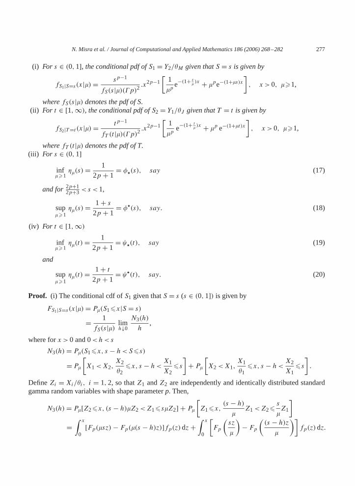
(i) For s ∈ (0,1], the conditional pdf ofS1 = Y2/�M given thatS = s is given by

fS1|S=s(x|�)= sp−1

fS(s|�)(p)2.x2p−1

[1

�pe−(1+ s

� )x + �pe−(1+�s)x], x >0, ��1,

wherefS(s|�) denotes the pdf of S.(ii) For t ∈ [1,∞), the conditional pdf ofS2 = Y1/�J given thatT = t is given by

fS2|T=t (x|�)= tp−1

fT (t |�)(p)2.x2p−1

[1

�pe−(1+ t

� )x + �p e−(1+�t)x], x >0, ��1,

wherefT (t |�) denotes the pdf of T.(iii) For s ∈ (0,1]

inf��1

��(s)= 1

2p + 1= �&(s), say (17)

and for 2p+12p+3 <s <1,

sup��1

��(s)= 1 + s

2p + 1= �&(s), say. (18)

(iv) For t ∈ [1,∞)

inf��1

��(t)= 1

2p + 1= �&(t), say (19)

and

sup��1

��(t)= 1 + t

2p + 1= �&(t), say. (20)

Proof. (i) The conditional cdf ofS1 given thatS = s (s ∈ (0,1]) is given by

FS1|S=s(x|�)= P�(S1�x|S = s)

= 1

fS(s|�) limh↓0

N3(h)

h,

where forx >0 and 0<h<s

N3(h)= P�(S1�x, s − h<S�s)

=P�

[X1<X2,

X2

�2�x, s − h<

X1

X2�s

]+ P�

[X2<X1,

X1

�1�x, s − h<

X2

X1�s

].

DefineZi = Xi/�i , i = 1,2, so thatZ1 andZ2 are independently and identically distributed standardgamma random variables with shape parameterp. Then,

N3(h)= P�[Z2�x, (s − h)�Z2<Z1�s�Z2] + P�

[Z1�x,

(s − h)

�Z1<Z2�

s

�Z1

]

=∫ x

0[Fp(�sz)− Fp(�(s − h)z)]fp(z)dz+

∫ x

0

[Fp

(sz

�

)− Fp

((s − h)z

�

)]fp(z)dz.


Therefore,

FS1|S=s(x|�)= 1

fS(s|�)[�

∫ x

0zf p(�sz)fp(z)dz+ 1

�

∫ x

0zf p

(sz

�

)fp(z)dz

].

Now the assertion follows on taking the derivative with respect toson both sides.(ii) Similar to the proof of (i).(iii) Suppose thats ∈ (0,1]. Then, note that

lim�↑∞ ��(s)= 1

2p + 1.

Therefore it is enough to show that

��(s)�1

2p + 1⇔ �s

[1

(s + �)2p+2 + 1

(1 + �s)2p+2

]�0,

which is always true.Therefore,

inf��1

��(s)= 1

2p + 1.

Now suppose that(2p + 1)/(2p + 3)< s <1. Note that

lim�↓1

��(s)= 1 + s

2p + 1.

Thus, it suffices to show that, for fixeds ∈ ((2p + 1)/(2p + 3),1),

��(s)�1 + s

2p + 1∀��1

⇔ �

(1 + �s

� + s

)2p+2

�1, ∀��1

⇔ ks(�)�0, ∀��1,

where, for fixeds ∈ ((2p + 1)/(2p + 3),1),

ks(�)= ln � + (2p + 2){ln(1 + �s)− ln(� + s)}, ��1.

Sinceks(1) = 0, it suffices to show that, for fixeds ∈ ((2p + 1)/(2p + 3),1), ks(�) is an increasingfunction of� ∈ [1,∞), i.e.

�

��ks(�)�0, ∀��1

⇔ vs(�)�0, ∀��1,

where, for fixeds ∈ ((2p + 1)/(2p + 3),1),

vs(�)= s�2 + {(2p + 3)s2 − (2p + 1)}� + s, ��1


is a quadratic equation with discriminant

� = [(2p + 3)s2 − (2p + 1)]2 − 4s2

= [(2p + 3)s + 2p + 1][(2p + 3)s − 2p − 1][s2 − 1].Clearly, for(2p+1)/(2p+3)< s <1, the discriminant�<0. Thus, it follows that, for(2p+1)/(2p+3)< s <1, vs(�)>0, ∀��1, which proves the required assertion.

(iv) Clearly, for fixedt�1,

lim�↑∞ ��(t)= 1

2p + 1

and

lim�↓1

��(t)= 1 + t

2p + 1.

Also, one can easily verify that

1

2p + 1��(t)�

1 + t

2p + 1,

which proves the required assertion.�

Now we will exploit the orbit by orbit improvement technique of Brewster and Zidek[3] to derive suf-ficient conditions for the inadmissibility ofequivariant estimatorsof �M and�J , under the loss functionsgiven by (1) and (2), respectively. Following theorem deals with the estimation of�M .

Theorem 21. Consider an estimator�1,�(Y ) = Y2�(S), belonging to the classDU of equivariant esti-mators of�M ; here�(.) is a real valued function defined on(0,1]. For �&(.) and�&(.), given by(17)and (18) respectively, suppose thatP�({S : �(S)<�&(S)} ∪ {S : �(S)>�&(S), S > (2p + 1)/(2p +3)})>0, ∀��1.Then,under the scale invariant squarederror loss function(1),the equivariant estimator�1,�(.) is inadmissible for estimating�M , and is dominated by�1,�1(Y )= Y2�1(S), where

�1(S)=

�&(S) if �(S)<�&(S)

�&(S) if �(S)>�&(S) and S >2p + 1

2p + 3�(S) otherwise.

Proof. For��1, consider the risk difference

1(�)= R1,�(�1,�)− R1,�(�1,�1)

=E�[S1�(S)− 1]2 − E�[S1�1(S)− 1]2=E�[S1{�(S)− �1(S)}{S1(�(S)+ �1(S))− 2}]=E�[D�(S)], say,

whereS1 = Y2/�M, S = Y1/Y2, and fors ∈ (0,1]D�(s)= (�(s)− �1(s))[(�(s)+ �1(s))E�(S

21|S = s)− 2E�(S1|S = s)].


We will establish that, for each��1,D�(s)�0, ∀s ∈ (0,1], with strict inequality on a set of positiveprobability. For this fixs ∈ (0,1]. On using Lemma 16 (i), we may write

D�(s)= C(s, �)(�(s)− �1(s))[�(s)+ �1(s)− 2��(s)],where��(s) is as defined in Lemma 16 and

C(s, �)= (2p + 2)

(p)2.�psp−1

fS(s|�)[

�2

(s + �)2p+2 + 1

(1 + �s)2p+2

].

Clearly, if �&(s)��(s)<�&(s) or �(s)��&(s) ands�(2p+ 1)/(2p+ 3), thenD�(s)= 0, ∀��1. For�(s)<�&(s)

D�(s)= C(s, �)(�(s)− �&(s))[�(s)+ �&(s)− 2��(s)]>0,

by Lemma 16 (iii) (see (17)).Now suppose that�(s)>�&(s) ands > (2p + 1)/(2p + 3). Then

D�(s)= C(s, �)(�(s)− �&(s))[�(s)+ �&(s)− 2��(s)]>0,

by Lemma 16 (iii) (see (18)).SinceP�({S : �(S)<�&(S)} ∪ {S : �(S)>�&(S), S > (2p + 1)/(2p + 3)})>0, ∀��1, the result

follows. �

Remark 22. (i) The result of above theorem fails to find an estimator dominating the estimator�1,c1(.).This estimator dominates the estimator�1,c0(.) (Remark 13 (i)) and it also dominates the UMVUE�1,�0(.) given by (5) (see[22]). We believe that the estimator�1,c1(.) is admissible within the classDUof equivariant estimators.

(ii) We know that the estimator�1,c0(.) is dominated by the estimator�1,c1(.). Theorem 21 providesanother dominating estimator for�1,c0(.), and it is given by

�&1,c0(Y )=

Y2

pif S�

2p + 1

2p + 3Y1 + Y2

2p + 1if S >

2p + 1

2p + 3.

Similarly, one can find another estimator that dominates the UMVUE�1,�0(.).

The following theorem deals with estimation of�J . The proof of the theorem follows on using Lemma16 (ii) and (iv) and proceeding on the lines of the proof of Theorem 17.

Theorem 23. Consider an estimator�2,�(Y ) = Y1�(T ), belonging to the classDL of equivariant esti-mators of�J ; here�(.) is a real valued function defined on[1,∞).For �&(.) and�&(.), given by(19)and(20) respectively, suppose thatP�({T : �(T )<�&(T )} ∪ {T : �(T )>�&(T )})>0, ∀��1.Then, underthe scale invariant squared error loss function(2), the equivariant estimator�2,�(.) is inadmissible forestimating�J , and is dominated by�2,�1(Y )= Y1�1(T ), where

�1(T )={

�&(T ) if �(T )<�&(T )�&(T ) if �(T )>�&(T )�(T ) otherwise.


Remark 24. (i) From Theorem 14, we know that forp�1 estimators�2,c0(.) and�2,c1(.) are not com-parable and both of these estimators are admissible within the subclassD1,L of equivariant estimators of�J . Using Theorem 23, one can obtain an estimator dominating the estimator�2,c0(.) for anyp>0. Thisestimator is given by

�&2,c0(Y )=

Y1

pif T >

p + 1

p

Y1 + Y2

2p + 1if T �

p + 1

p.

However, Theorem 23 fails to improve upon the estimator�2,c1(.), which we believe is admissible in theclassDL of equivariant estimators of�J .

(ii) Theorem 23 also provides an estimator dominating the UMVUE�2,�0(.), given by (6).A dominatingestimator is given by

�&2,�0(Y )=

Y1

p

[1 +

(Y1

Y2

)p−1]

if T > t0

Y1 + Y2

2p + 1if T � t0,

wheret0 ∈ [1,∞) is the root of the equation

ptp − (p + 1)tp−1 − (2p + 1)= 0.

(iii) It will be interesting to extend the results of this paper to the case ofk (�2) gamma populations.

Acknowledgements

The research of the first author was supported by a fellowship awarded by the research council ofthe Katholieke University Leuven (Belgium), while the research of the second author was supported byF.W.O. Flanders Research Grant No. 1.5593.98N.

References

[1] N.K. Bansal, K.J. Miescke, K.J. Simultaneous selection and estimation in general linear models, Preprint, 2001.[2] N.K. Bansal, N. Misra, E.C. van der Meulen, On minimax decision rules in ranking problems, Statist. Prob. Lett. 34 (1997)

179–186.[3] J.F. Brewster, Z.V. Zidek, Improving on equivariant estimators, Ann. Statist. 2 (1974) 21–38.[4] A. Cohen, H. Sackrowitz, A decision theory formulation for population selection followed by estimating the mean of the

selected population, in: S.S. Gupta, J.O. Berger (Eds.), Statistical Decision Theory and Related Topics-IV, vol. 2, Springer,New York, 1988, pp. 33–36.

[5] R.C. Dahiya, Estimation of the mean of the selected population, J. Amer. Statist. Assoc. 69 (1974) 226–230.[6] M.L. Eaton, Some optimum properties of ranking procedures, Ann. Math. Statist. 38 (1967) 124–137.[7] S.S. Gupta, K.J. Miescke, On finding the largest normal mean and estimating the selected mean, Sankhya B 52 (1990)

144–157.[8] S.S. Gupta, K.J. Miescke, On combining selection and estimation in the search for the largest, J. Statist. Planning Inference

36 (1993) 129–140.


[9] H. Hseih, On estimating the mean of the selected population with unknown variance, Comm. Statist.—Theor. Meth. 10(1981) 1869–1878.

[10] S. Jeyaratnam, S. Panchapakesan, Estimation after subset selection from exponential populations, Comm. Statist.—Theor.Meth. 15 (1986) 3459–3473.

[11] N. Misra, Estimation of the average worth of the selected subset of gamma populations, Sankhya, Ser. B 56 (1994)344–355.

[12] N. Misra, G.N. Singh, On the UMVUE for estimating the parameter of the selected exponential population, J. IndianStatist. Assoc. 31 (1993) 61–69.

[13] J. Putter, D. Rubinstein, On estimating the mean of a selected population, Technical Report No. 165, Department ofStatistics, University of Wisconsin, 1968.

[14] H.B. Sackrowitz, E. Samuel-Cahn, Estimation of the mean of a selected negative exponential population, J. Roy. Statist.Soc. Ser. B 46 (1984) 242–249.

[15] H. Sackrowitz, E. Samuel-Cahn, Evaluating the chosen population : a Bayes and minimax approach, in: John van Ryzin(Ed.),Adaptive Statistical Procedures and RelatedTopics, IMS Lecture Notes, Monograph Series, 1987, vol. 8, pp. 386–399.

[16] K. Sarkadi, Estimation after selection, Studia Scientarium Mathematicarum Hungarica 2 (1967) 341–350.[17] R. Song, On estimating the mean of selected uniform population, Comm. Statist.—Theor. Meth. 21 (1992) 2707–2719.[18] P. Vellaisamy, Inadmissibility results for the selected scale parameter, Ann. Statist. 20 (1992) 2183–2191.[19] P. Vellaisamy, Average worth and simultaneous estimation of the selected subset, Ann. Inst. Statist. Math. 44 (1992)

551–562.[20] P. Vellaisamy, On UMVU estimation following selection, Comm. Statist.—Theor. Meth. 22 (1993) 1031–1043.[21] P. Vellaisamy, A note on estimation of the selected parameters, J. Statist. Planning Inference 55 (1996) 39–46.[22] P. Vellaisamy, D. Sharma, Estimation of the mean of the selected gamma population, Comm. Statist.—Theor. Meth. 17

(1988) 2797–2817.[23] P. Vellaisamy, D. Sharma, A note on the estimation of the selected gamma population, Comm. Statist.—Theor. Meth. 18

(1989) 555–560.

Documents

On estimating the scale parameter of the selected gamma population under the scale invariant squared error loss function