Embed Size (px)
Citation preview

DPRIETI Discussion Paper Series 08-E-015
On Equivalence Results in Business Cycle Accounting
NUTAHARA Kengothe University of Tokyo, and JSPS
INABA MasaruRIETI
The Research Institute of Economy, Trade and Industryhttp://www.rieti.go.jp/en/

RIETI Discussion Paper Series 08-E-015
On Equivalence Results in Business Cycle Accounting
Kengo Nutahara* and Masaru Inaba†
Revised: September 2008
Abstract Business cycle accounting rests on the insight that the prototype neoclassical growth model with
time-varying wedges can achieve the same allocation generated by a large class of frictional models:
equivalence results. Equivalence results are shown under general conditions about the process of
wedges while it is often specified to be the first order vector autoregressive when one applies
business cycle accounting to actual data. In this paper, we characterize the class of models covered
by the prototype model under the conventional first order vector autoregressive specification of
wedges and find that it is much smaller than that believed in previous literature. We also apply
business cycle accounting to an artificial economy where the equivalence does not hold and provide
a numerical example that business cycle accounting works well even in such an economy.
Keywords: Equivalence results; business cycle accounting
JEL Classification: E32
* University of Tokyo, and JSPS research fellow † Research Institute of Economy, Trade and Industry (RIETI)
On Equivalence Results in Business Cycle Accounting∗
Kengo Nutahara
Graduate School of Economics, the University of Tokyo
7-3-1 Hongo, Bunkyo-ku, Tokyo 113-0033 Japan
Masaru Inaba
Research Institute of Economy, Trade and Industry
Daidoseimei-Kasumigaseki Building 20th Floor
1-4-2 Kasumigaseki, Chiyoda-Ku, Tokyo 100-0013 Japan
Revised: September 2008
∗We would like to thank Richard Anton Braun, Fumio Hayashi, Julen Esteban-Pretel, KeiichiroKobayashi, Koji Miyawaki, Kensuke Miyazawa, Tomoyuki Nakajima, Keisuke Otsu, Hikaru Saijo, Fumi-hiko Suga, and seminar participants at the Research Institute of Economy, Trade and Industry (RIETI)for their helpful comments. The first author is particularly grateful to Kensuke Miyazawa for valuablediscussions on this topic. Of course, the remaining errors are our own.
1

Abstract
Business cycle accounting rests on the insight that the prototype neoclassical
growth model with time-varying wedges can achieve the same allocation generated
by a large class of frictional models: equivalence results. Equivalence results are
shown under general conditions about the process of wedges while it is often specified
to be the first order vector autoregressive when one applies business cycle accounting
to actual data. In this paper, we characterize the class of models covered by the pro-
totype model under the conventional first order vector autoregressive specification of
wedges and find that it is much smaller than that believed in previous literature. We
also apply business cycle accounting to an artificial economy where the equivalence
does not hold and provide a numerical example that business cycle accounting works
well even in such an economy.
Keywords: Business cycle accounting; equivalence results
JEL classification: C68, E10, E32
2

1 Introduction
Business cycle accounting (hereafter BCA) is a method that is used (i) to measure dis-
tortions by the prototype model with time-varying wedges, which resemble aggregate
productivity, labor and investment taxes, and government consumption, such that the
prototype model perfectly accounts for observed data, and (ii) to investigate the im-
portance of each wedge in business cycles by counterfactual simulations. In order to
substantiate their prototype model, Chari, Kehoe and McGrattan (2007a) (hereafter
CKM) claim equivalence results – namely, their prototype model covers a large class of
frictional detailed business cycle models. Equivalence results suggest that the prototype
model is equivalent to a detailed model if and only if the first order conditions of the
prototype model are satisfied given any allocation of consumption, investment, labor,
and output generated by the detailed model through the adjustment of wedges. CKM
show equivalence results under general conditions about evolutions of wedges. However,
in practice, they impose that wedges evolve according to the first order vector autore-
gressive, VAR(1), process and it is not clear whether CKM’s VAR(1) specification of
wedges is consistent with conditions in terms of equivalence results. Many papers that
apply BCA also employ CKM’s VAR(1) specification of wedges. Therefore, it is impor-
tant to investigate the class of models covered by the prototype model with the VAR(1)
specification of wedges. And if the class of models covered by the prototype model is
small, it is also important to investigate whether or not BCA can measure true wedges
in an economy where equivalence result does not hold. Non equivalence might lead a
mismeasurement of wedges. In the literature of BCA, there are two opposite results
on the importance of investment wedge for business cycles and these results depend on
minor difference in the procedure of BCA. The diversion of results might be accounted
for by the non equivalence between the prototype model and the true model of the real
world.
In this paper, we examine the equivalence results by focusing on the VAR(1) represen-
tation of wedges. We characterize the class of frictional models covered by the prototype
model with the conventional VAR(1) specification of wedges. We find that the prototype
3

model covers a detailed model if and only if wedges have sufficient information about
the endogenous and exogenous states of the detailed model. Intuitively, the number of
independent wedges should be larger than that of endogenous and exogenous states vari-
ables in the detailed model. We also find that the class covered by the prototype model
is much smaller than that is shown in CKM under general conditions of wedges. Some
examples of the equivalence in CKM are not covered by the prototype model with the
VAR(1) specification of wedges. Therefore, the condition for equivalence results is highly
restrictive if we employ the VAR(1) representation of wedges. We extend our analysis to
an alternative specification which has the VAR(1) specification as a special case and find
that the class of models covered by the prototype model is not so large even in such case.
We also apply BCA to an artificial medium-scale dynamic stochastic general equilibrium
(hereafter DSGE) model, which is not covered by the prototype model, in order to assess
the empirical usefulness of BCA. We provide an example that measured wedges capture
the properties of the true wedges almost correctly even in such an economy. There-
fore, our result tells us that even if the prototype model is not equivalent to a detailed
model, BCA might work well since the prototype model is as a good approximation of
the detailed model.
In the following, we describe the related literature. CKM propose BCA and claim that
their prototype model covers a large class of frictional business cycle models.1 CKM also
conclude that investment wedge is not promising for business cycle research. Christiano
and Davis (2006) critique the procedure of BCA and claim that results of BCA are fragile
if they employ an alternative procedure.2 This paper is closely related to Baeurle and
Burren (2007). They investigate the class of frictional models covered by the prototype
model and their study was conducted at the same time as this paper. We show the class
of models which are equivalent to the prototype model while they consider only the class
of models where there exists the VAR(1) specification of wedges, which is a necessary1Chari, Kehoe, and McGrattan (2002) apply BCA using the deterministic prototype model. In the
case of the deterministic prototype model, there is no theoretical problem of equivalence results. However,when we implement BCA in the deterministic economy, we have to assume the future path of wedgesand such assumption might cause mismeasurement of wedges.
2Chari, Kehoe, and McGrattan (2007b) critique the alternative procedure of Christiano and Davis(2006).
4

condition for the equivalence.
The rest of this paper is as follows. Section 2 introduces the basic framework for the
analysis: the prototype model, a detailed model, and the definition of the equivalence.
Section 3 presents our main results. We characterize the class of models covered by the
prototype model with the VAR(1) specification of wedges and discuss implications of our
results. We extend our analysis to more general class of the process of wedges in Section
4. In Section 5, we apply BCA to an artificial economy where the equivalence result
does not hold and provide a numerical example that BCA can measure wedges almost
correctly even in such an economy. Section 6 draws certain concluding remarks.
2 Basic Setting
2.1 Prototype Model
The prototype economy of the equivalence result is as follows.3 The representative house-
hold problem is given by the following:
maxct,ℓt,it
E0
∞∑t=0
βt
[log(ct) + ν log(1 − ℓt)
], (1)
s.t. ct + (1 + τx,t)it ≤ (1 − τℓ,t)wtℓt + rtkt−1 − Tt, (2)
kt = (1 − δ)kt−1 + it, (3)
where ct denotes consumption; ℓt, labor supply; τx,t, imaginary investment tax; 1/(1 +
τx,t), investment wedge; τℓ,t, imaginary labor income tax; (1 − τℓ,t), labor wedge; it,
investment; wt, wage rate; rt, rental rate of capital; kt−1, capital stock at the end of
period t; and Tt, the lump-sum tax.
The production function of competitive firms is
yt = Atkαt−1ℓ
1−αt , (4)
3While CKM consider a general model with histroty dependence, we restrict a model which has therecursive structure in the present paper.
5

where yt denotes output, and At denotes efficiency wedge.4 Finally, the market clearing
condition is
ct + it + gt = yt, (5)
where gt denotes government wedge.
The equilibrium system of the prototype model is summarized as
νct
1 − ℓt= (1 − τℓ,t)(1 − α) · yt
ℓt, (6)
1 + τx,t
ct= βEt
[1
ct+1
(1 + τx,t+1)(1 − δ) + α
yt+1
kt
], (7)
yt = Atkαt−1ℓ
1−αt , (8)
kt = (1 − δ)kt−1 + it, (9)
ct + it + gt = yt, (10)
where (6) denotes the consumption-leisure-choice optimization condition; (7), the Euler
equation; (8), the aggregate production function; (9), the evolution of aggregate capital
stock; (10), the resource constraint. To close the model, we have to specify the evolution
of wedges. CKM specify that the vector of wedges st ≡ [log(At), τℓ,t, τx,t, log(gt)]′ evolves
according to the first order vector autoregressive, VAR(1), process as
st+1 = P 0 + Pst + εt+1, (11)
where εt is i.i.d. over time and is normally distributed with mean zero.
CKM also consider the prototype model with capital wedge, which resembles to capital
income tax, instead of investment wedge. In this case, the budget constraint (2) becomes
ct + it ≤ (1 − τℓ,t)wtℓt + (1 − τk,t)rtkt−1 − Tt, (12)
4We consider a stationary economy for simplicity.
6
where (1 − τk,t) denotes capital wedge. The analogue of (7) is
1ct
= βEt
[1
ct+1
(1 − δ) + (1 − τk,t+1)α
yt+1
kt
], (13)
and st ≡ [log(At), τℓ,t, τk,t, log(gt)]′.5 We consider the case of the prototype model with
investment wedge in this paper, but the analogues of results in Section 3 are applicable
to the prototype model with capital wedge.
2.2 Detailed and Extended Detailed Models
Here, we define two models: a detailed model and an extended detailed model for the
analysis.
Let xt be a vector of the endogenous state variables; yt, a vector of endogenous jump
variables; and zt, a vector of exogenous state variables. let n and q is the numbers of
variables contained in [x′t−1, z
′t]′ and yt, respectively. We consider these variables to be
defined as deviations from the deterministic steady-state.
As in Uhlig (1999), generally, a linearized DSGE detailed model is described as
Axt + Bxt−1 + Cyt + Dzt = 0, (14)
Et
[Fxt+1 + Gxt + Hxt−1 + Jyt+1 + Kyt + Lzt+1 + Mzt
]= 0, (15)
zt+1 = Nzt + ut+1, Et
[ut+1
]= 0, (16)
where ut+1 is i.i.d. over time and is normally distributed with mean zero. We assume
that consumption ct, investment it, labor ℓt, capital stock kt, and output yt are definable
in this detailed model and that capital stock at the beginning of period kt−1 is included
5CKM employ some types of capital wedge. This version is employed for equivalence result of theinput-financing friction model as we will show in Section 3.
7

in xt−1. The state-space form solution of this detailed model is
xt
zt+1
= Ψ
xt−1
zt
+
0
ut+1
, (17)
yt = Ω
xt−1
zt
, (18)
where Ψ is an n × n matrix and Ω is a q × n matrix. The aggregate decision rule of
consumption, investment, labor, output, and capital stock at the end of period is
ct
it
ℓt
yt
kt
= Θ
xt−1
zt
, (19)
where Θ is a 5 × n matrix and variables with hat ˆ denote (log) deviations from the
deterministic steady-state.
Here, we introduce the extended detailed model in order to consider wedges which are
consistent with the detailed model as follows.
Definition 1. An extended detailed model consists of (i) a equilibrium system of a de-
tailed model (14), (15), and (16), and (ii) the linearized equations of the first order
conditions of the prototype model (6), (7), (8), (9), and (10).
The extended detailed model implies that any realized sequences of consumption,
investment, labor, and output generated by the detailed model are consistent with the
first order conditions of the prototype model (6), (7), (8), (9), and (10). Since st is
the endogenous variables in the extended detailed model, we can calculate the aggregate
8

decision rule of st as
st = Φ
xt−1
zt
, (20)
where Φ is an m×n matrix; m, the number of wedges st; and n, the number of endogenous
and exogenous state variables [x′t−1,z
′t]′.6 We are also able to calculate the aggregate
decision rule of endogenous and exogenous state variables as
xt
zt+1
= Ψ
xt−1
zt
+
0
ut+1
, (21)
where Ψ is an n × n matrix.
2.3 Equivalence Results
The definition of the equivalence is as follows.
Definition 2. The prototype model is equivalent to (or covers) a detailed model if the
prototype model can achieve any realized sequences of consumption, investment, labor,
output, and capital stock generated by the detailed model.
In other words, the prototype model is equivalent to a detailed model if the intratem-
poral condition (6), the Euler equation (7), the aggregate production function (8), and
the resource constraint (10) are satisfied given any realized sequences of ct, it, ℓt, yt, kt
generated by the detailed model. These four equations are satisfied by suitable adjust-
ments of wedges. CKM claim equivalence results by comparing the first order conditions
of two models and derivate conditions where the first order conditions of the detailed
model are identical to (6), (7), (8), (9), and (10) in some examples. Their equivalence
results are true under general conditions about process of wedges. However, in practice,
CKM impose that wedges evolve according to VAR(1) and it is not clear whether or not
VAR(1) specification of wedges is consistent with such conditions. It is also unclear that6We assume that this extended detailed model satisfies the suitable conditions in order to solve the
aggregate decision rule, that is, the Blanchard-Kahn condition.
9

even if such VAR(1) specification exists, the prototype model is equivalent to a detailed
model in general.
Generally, the necessary and sufficient condition of the equivalence is summarized as
follows.
Proposition 1. The prototype model is equivalent to a detailed model if and only if (i)
a process of wedges to close the prototype model is consistent with the detailed model,
and (ii) there exists, in the extended detailed model, a mapping from the states of the
prototype model given the process of wedges to variables of the prototype model.
The necessity of (i) is obvious since it is needed to close the prototype model. The
necessity of (ii) is as follow. There exists, in the prototype model, a mapping from the
states to variables and if the condition (ii) does not hold, realized sequences of variables
generated by the detailed model are not achieved in the prototype model. The sufficiency
is also easily shown as follows. The mapping (ii) generated in the extended detailed model
must satisfy the first order conditions of the prototype model since they are also included
in the extended detailed model.7 Note that the condition (ii) requires that the state-space
form solution of the prototype model must exists in the extended detailed model.
We investigate these problems through a formal discussion of the linearized economy
in the following two sections.8 In Section 3, we consider the case of the VAR(1) specifi-
cation of wedges. We extend our analysis to an alternative specification which has the
VAR(1) specification as a special case in Section 4.
7Baeurle and Burren (2007) consider only the problem about (i). One of contributions of the presentpaper is to consider the condition (ii).
8We only consider a linearized economy. However, results in this paper hold in a non-linear economyin the neighborhood of a steady-state.
10

3 VAR(1) Specification of Wedges
3.1 Conditions for Equivalence
In the case of CKM’s VAR(1) specification (11), the condition (i) is the existence of
st+1 = P st + εt+1, (22)
in the extended detailed model. Since, in the case of VAR(1) specification of wedges,
[kt−1, s′t]′ are the state variables in the prototype model, the condition (ii) is the existence
of the mapping from [kt−1, s′t]′ to consumption, investment, labor, output and capital
stock at the end of period:
ct
it
ℓt
yt
kt
= Λ
kt−1
st
, (23)
where Λ is a 5 × (n + 1) matrix, in the extended detailed model. Note that we do not
need to consider the existence of the mapping from [kt−1, s′t]′ to st+1 if the VAR(1)
specification of wedges (22) exists.
First, we consider the existence of the VAR(1) specification of wedges. The necessary
and sufficient condition for the existence of the VAR(1) representation is as follows.
Lemma 1. Assume that (20) and (21) hold in the extended detailed model. There exists
P that satisfies CKM’s specification (22) if and only if
rank(Φ) = rank
( [Φ′ ... Ψ′Φ′
] ). (24)
Proof. See Appendix A.
If rank(Φ) = n, the following Lemma 1 holds and provides us with some intuitions
11

with regard to the existence of P .
Lemma 2. Assume that (20) and (21) hold in the extended detailed model. If the rank
of Φ equals the number of endogenous and exogenous states in the detailed model, n,
there exists P that satisfies CKM’s specification (22).
Proof. Since rank(Φ) = n, there exists (Φ′Φ)−1. Then, (20) becomes
(Φ′Φ)−1Φ′st =
xt−1
zt
. (25)
By (25) and (21), we obtain
st+1 = ΦΨ(Φ′Φ)−1Φ′st + Φ
0
ut+1
. (26)
Therefore, there exists a VAR(1) representation of wedges (22) where P = ΦΨ(Φ′Φ)−1Φ′
and εt+1 = Φ[0, u′t+1]
′.
Lemma 2 can be interpreted as follows. As seen in (25), rank(Φ) = n implies that
[x′t−1 z′
t]′ are identified by st if we know Φ. In other words, wedges st has sufficient
information with regard to the endogenous and exogenous states [x′t−1 z′
t]′, and such
wedges can be written as a VAR(1) process. Intuitively, the number of independent
wedges should be that of endogenous and exogenous state variables in the detailed model
at least in order to let the prototype model cover the detailed model. It is easily shown
that, in general, P does not exist if rank(Φ) < n. Generally, if the number of wedges is
strictly smaller than that of the endogenous and exogenous states in the detailed model
or n > m, wedges cannot contain adequate information regarding the endogenous and
exogenous states in general. Then, there is no VAR(1) representation of wedges. Even
if the number of wedges are larger than that of the endogenous and exogenous states in
the detailed model or m ≥ n, and if rank(Φ) < n, it implies that wedges do not have
sufficient information about the endogenous and exogenous states in the detailed model,
and there is no VAR(1) representation in general.
12
Next, we consider the existence of (23). Let a (m + 1) × n matrix Φ to be
Φ =
e
Φ
, (27)
where e = [1, 0, 0, · · · , 0] is a 1 × n vector and it satisfies
kt−1
st
= Φ
xt−1
zt
. (28)
The necessary and sufficient condition for the existence of (23) is as follows.
Lemma 3. Assume that (20) and (28) hold in the extended detailed model. There exists
Λ that satisfies (23) if and only if
rank(Φ) = rank
( [Φ
′ ... Θ′] )
. (29)
Proof. See Appendix B.
If rank(Φ) = n, the following Lemma 4 holds and provides us with some intuitions
with regard to the existence of Λ.
Lemma 4. Assume that (19) and (20) hold in the extended detailed model. If the rank
of Φ equals the number of endogenous and exogenous states in the detailed model, n,
there exists Λ that satisfies (23).
Proof. Since rank(Φ) = n, there exists (Φ′Φ)−1 and
xt−1
zt
=(Φ
′Φ
)−1Φ
′
kt−1
st
. (30)
By (19) and (30), it is easily shown that Λ = Θ(Φ
′Φ
)−1Φ
′is a solution.
It is easily shown that, in general, Λ does not exist if rank(Φ) < n as in the case of
P . Roughly speaking, if the number of wedges plus one is strictly smaller than that of
13

the endogenous and exogenous states in the detailed model or n > m+1, wedges cannot
contain adequate information regarding the endogenous and exogenous states in general.
Then, there is no mapping from [kt−1, s′t]′ to consumption, investment, labor, output,
and capital stock.
Finally, the necessary and sufficient condition for the equivalence is summarized as
follow.
Theorem 1. Assume that (19), (20), (21), and (28) hold in the extended detailed model.
The prototype model with the VAR(1) specification of wedges is equivalent to the detailed
model if and only if
rank(Φ) = rank
( [Φ′ ... Ψ′Φ′
] ), (31)
rank(Φ) = rank
( [Φ
′ ... Θ′] )
. (32)
Proof. It is obvious by Lemma 1 and 3.
The following sufficient condition is useful to understand the intuition.
Theorem 2. Assume that (19), (20), (21), and (28) hold in the extended detailed model.
The prototype model with the VAR(1) specification of wedges is equivalent to the detailed
model if the rank of Φ equals the number of endogenous and exogenous states in the
detailed model, n.
Proof. It is obvious by Lemma 2, 4 and that rank(Φ) = n implies rank(Φ) = n.
Theorem 2 implies the sufficient condition of the existence of the VAR(1) representa-
tion of wedges rank(Φ) = n is the sufficient conditions of the existence of the mapping
from the states of the prototype model to consumption, investment, labor, capital, and
output in the extended detailed model. The prototype model is equivalent to a detailed
model if the VAR(1) representation of wedges exists in many cases. This tells us that, in
the case of VAR(1) of wedges, the condition (ii) is less restrictive. We will show that the
condition (ii) is restrictive when we introduce an alternative specification of the process
of wedges in Section 4.
14

3.2 Implications of Our Results
We showed that the VAR(1) representation of wedges exists if and only if wedges have
sufficient information about the endogenous and exogenous states in the detailed model
and that equivalence holds in many cases if the VAR(1) representation exists. We can
roughly verify the condition for the existence of P by comparing the number of wedges m
and that of endogenous and exogenous states n of the detailed model. If rank(Φ) < n,
there is no P in general. If the detailed model is a medium-scale DSGE model of
the current generation, which has many exogenous shocks and endogenous states, the
equivalence results do not hold in many cases since the maximum number of wedges is
at most four.
Even if the number of endogenous and exogenous states is small, a VAR(1) represen-
tation might not exist. Here, we show that the class of frictional models covered by the
prototype model with the VAR(1) specification of wedges is much smaller than that is
shown in CKM under general conditions of wedges.
The sticky-wage model in CKM is not covered by the associated prototype model.
In their sticky-wage model, the endogenous state is aggregate capital kt−1 and the ex-
ogenous state is money supply Mt. In the associated prototype model, there is only
one wedge – labor wedge, or rank(Φ) = 1. Then, according to Lemma 1, a VAR(1)
representation does not exist in general since the number of wedges is strict smaller than
that of endogenous and exogenous variables: m < n.
The input-financing friction model in CKM is also not covered by the associated
prototype model. The endogenous state is aggregate capital kt−1, and the exogenous
states are the interest rate spreads of sector 1 and 2: τ1,t and τ2,t in the model with
input-financing friction.9 In the associated prototype model, there are three wedges –
efficiency, labor, and capital wedges. Subsequently, in this case, n = m in this case;
9CKM do not specify what are exogenous shocks. Here, we consider two interest rate spreads areexogenous shocks to close the model.
15

however CKM’s Proposition 1 shows that τℓ,t equals τk,t. This implies that
st = Φ
xt−1
zt
⇐⇒
log(At)
τℓ,t
τk,t
=
ϕ1,1 ϕ1,2 ϕ1,3
ϕ2,1 ϕ2,2 ϕ2,3
ϕ3,1 ϕ3,2 ϕ3,3
kt−1
τ1,t
τ2,t
, (33)
where ϕ2,i = ϕ3,i for i = 1, 2, and 3. It is obvious that rank(Φ) = 2 < 3 = n in general,
and then there is no VAR(1) representation.10 These results imply that equivalence
result is highly restrictive under the VAR(1) specification of wedges.
Note that the equivalence depends on the whole structure of a detailed model, not
only frictions. We show that CKM’s sticky-wage model is not covered by the prototype
model with the VAR(1) specification of wedges, however, this does not mean that all
models with sticky-wage are not covered by the prototype model. For example, if the
sticky-price model with only technology shocks, not money supply, the prototype model
is equivalent to it since the number of endogenous and exogenous variables are two:
capital stock and technology, and the number of wedges are two: efficiency and labor
wedges.
4 Alternative Specification of Wedges
In Section 3, we consider the case of the VAR(1) specification of wedges. Here, we
consider an alternative specification of wedges, which lets the prototype model cover
larger class of frictional models than that in the case of the VAR(1) representation. We
will show that the prototype model with our alternative specification can cover larger
class of models but such class is not so large.
Let πt is a r × 1 vector of variables included in both the prototype model and the
10This non equivalence arises since the prototype model is described by capital wedge as in (13). Theprototype model with investment wedge is equivalent to this input-financing friction model.
16

detailed model such that
πt = Ξ
xt−1
zt
, (34)
where Ξ is an r×n matrix. Then, a candidate of variables included in πt is jump or state
variables at period t in the extended detailed model. Consider the following alternative
specification:
st+1 = R0 + Rπt + ηt+1, (35)
where R0 is an m × 1 vector, R is an m × r matrix, and ηt+1 is i.i.d. over time and is
normally distributed with mean zero. Note that the VAR(1) specification of wedges (11)
is a special case of (35) where πt = st. The linearized version of (35) is
st+1 = Rπt + ηt+1. (36)
Even if we do not specify variables in πt, we can discuss about the existence of (36) by
(34). The necessary and sufficient condition is as follows.
Lemma 5. Assume that (20), (21) and (34) hold in the extended detailed model. There
exists R that satisfies our specification (36) if and only if
rank(Ξ) = rank
( [Ξ′ ... Ψ′Φ′
] ). (37)
Proof. It is easily shown that there exists R that satisfies RΞ = ΨΦ if and only if (37)
holds. The rest of the proof is almost similar to that in the proof of Lemma 1. Necessity
and sufficiency are easily shown.
Lemma 5 is the analogue of Lemma 1. The analogue of Lemma 2 is as follows.
Lemma 6. Assume that (20), (21), and (34) hold in the extended detailed model. If the
rank of Ξ equals the number of endogenous and exogenous states in the detailed model,
17
n, there exists a unique R that satisfies the alternative specification (36).
Proof. It is easily shown by the same logic in the proof of Lemma 2.
These lemmas imply that our specification (35) holds if and only if πt has sufficient
information about the endogenous and exogenous states in the detailed model. Roghly
speaking, if the number of πt is larger than that of the endogenous and exogenous states
in the detailed model, there exists (35).
The rest is the condition (ii) in Proposition 2. To consider it, we have to specify πt.
Specification of Baurle and Burren (2007): A candidate of the specification of πt
is as follows.
πt ≡
kt−1
st
. (38)
where kt−1 is the “aggregate” capital stock and kt−1 = kt−1 in equilibrium. This “aggre-
gate” trick is employed in order to let the first order conditions of the prototype model to
be same (6), (7), (8), (9), and (10). This specification of πt is the same as that proposed
in Baurle and Burren (2007).
Since, under the specification (36), the state variables of the prototype model is
[kt−1, s′t]′ and the condition (ii) in Proposition 1 is the same as (23). Therefore, Lemma
3 and 4 is applicable. In the case of this alternative specification, the necessary and
sufficient condition for the equivalence is summarized as follow.
Theorem 3. Assume that (19), (20), (21), and (28) hold in the extended detailed model.
The prototype model with the specification of wedges :
st+1 = R0 + Rπt + ηt+1,
18

where
πt ≡
kt−1
st
is equivalent to the detailed model if and only if
rank(Ξ) = rank
( [Ξ′ ... Ψ′Φ′
] ), (39)
rank(Φ) = rank
( [Φ
′ ... Θ′] )
. (40)
Proof. It is obvious by Lemma 3 and 5.
In this case of the specification, Ξ = Φ and the sufficient condition for the existence
of the alternative specification (36), Ξ, implies the condition (23): the mapping from the
states of the prototype model to variables. Thus, the equivalence holds if the existence
of the alternative specification (36) exists in many cases.
Since there are m + 1 variables in πt, this alternative specification exists in the
case where the number of endogenous and exogenous states is smaller than m + 1 in
the detailed model. It is easily verified that the prototype model with this specification
covers CKM’s sticky-wage model and the input-financing friction model shown in Section
3.
Note that the equivalence depends on the whole structure of a detailed model, not
only frictions as explained in Section 3. CKM’s sticky-wage model is not covered by
the prototype model with alternative specification of wedges (36) and (38), however, it
does not mean that all sticky-wage models are covered. The equivalence depends on
the number of independent state variables in the detailed model. Note also that the
prototype model with this specification, generally, can only cover a detailed model in
which the number of the state variables is less than five. Medium-scale DSGE models
in the current generation, like Christiano, Eichenbaum, and Evans (2005), cannot be
covered since there are many endogenous and exogenous variables.
19

Even if we augment πt... Consider the case where there are more variables in πt.
For example,
πt ≡
kt−1
st
ct
, (41)
where ct is aggregate consumption and ct = ct in equilibrium. We augment the previous
specification of πt by ct.
The alternative specification exists even if the number of the endogenous and exoge-
nous wedges is six, which is the specification of Baurle and Burren (2007) does not exist.
However, the class of detailed models covered by the prototype model with this specifi-
cation is not larger than that covered by the prototype model with the specification of
Baurle and Burren (2007) since the condition (ii) in Proposition 1 is restrictive. In this
specification, the condition (ii) in Proposition 1 is the same as (23). It is described as in
Proposition 2.
Proposition 2. If a detailed model is covered by the prototype model with the alternative
specification (35) and πt ≡ [kt−1, s′t, ct]′, it is also covered by the prototype model with
(35) and πt ≡ [kt−1, s′t]′.
Proof. Assume that a detailed model is covered by the prototype model with (36) and
(41). Then, (23) and
st+1 = R
kt−1
st
ct
+ ηt (42)
hold. Since there is a mapping from [kt−1, s′t]′ to ct, (42) is rewritten as
st+1 = R
kt−1
st
+ ηt. (43)
20

(23) and (43) imply that this detailed model is covered by the prototype model with (36)
and (41).
The analogue of Proposition 2 holds if we augment πt by other variables in the pro-
totype model. Therefore, generally, the number independent endogenous and exogenous
variables in detailed models covered by the prototype model with (35) is less than six
and the class of detailed models is not so large.11
5 Business Cycle Accounting without Equivalence
We showed that equivalence results is highly restrictive and the class of models covered
by the prototype model with the VAR(1) specification is small in previous two sections.
However, there is a possibility that the prototype model works well as an approximation
of the detailed model. In this section, we investigate what happens if we apply BCA to
an economy where the equivalence result does not hold in order to assess the usefulness
of BCA.12 We provide an example that measured wedges capture the properties of the
true wedges almost correctly even if the equivalence does not hold.
5.1 An artificial economy
We employ a kind of medium-scale DSGE model as in Christiano, Eichenbaum, and
Evans (2005).13 The reason why we employ medium-scale DSGE model is that such
model has rich enough dynamics to produce the actual tendency found in the data and
we already know the empirically plausible range of parameters in this sort of models.
So, using this model, we can investigate the empirical usefulness of BCA under plausible
parameter values in a realistic economy.
11It is well-known that the VARMA representation exists under more general conditions than VAR(1)by the VAR literature as in Ravenna (2007). One of our future tasks is to investigate the case of theprototype model with the VARMA representation of wedges.
12In the literature of the structural VARs, Ravenna (2007) and Christiano, Eichenbaum, and Vigfusson(2006) investigate the empirical usefulness of VARs by applying VARs to artificial economies.
13The details about our model and our parameter values are described in Appendix C.
21

Our model has the following properties: (i) sticky price with backward price index-
ation, (ii) sticky wage with backward price indexation, (iii) habit persistence, and (iv)
forward-looking Taylor rule. In our model, there are seven independent endogenous and
exogenous state variables and both prototype models with VAR(1) specification and
alternative specification with πt ≡ [kt−1, s′t]′ cannot cover this model. We eliminate
adjustment cost of investment since there is no adjustment cost in the prototype model
for BCA in Section 2. 14 The parameter values of our medium-scale DSGE model are
described in Table 1. We specify the model to be quarterly. We employ the log-linear ap-
proximation to calculate the aggregate decision rule and generate 200 periods (50 years)
artificial data.
5.2 Business cycle accounting
Our procedure of BCA follows the standard way. We set the parameter values of the
prototype model as follows: discount factor β, depreciation rate of capital δ, and share of
capital in production α to be the same as in our detailed model, and the weight of leisure
in utility ν to be 2.15 We employ the Bayesian method based on the Kalman filter to
estimate the process of wedge P .16 Table 2 shows prior distributions of the parameters
and Table 3 shows posterior distributions. Given the evolution of wedges P , wedges are
measured by
idt
ℓdt
ydt
= Λ
kdt−1
st
, (44)
kt = (1− δ)kt−1 + δidt , k−1 = kd−1, and gt = gd
t , where variables with superscript d denote
actual data and Λ is 3× 5 matrix. There are three equations and three unknown wedges14While the adjustment costs of investment is one of important feature in the medium-scale DSGE
models, we eliminate it. To investigate the case of the prototype model with adjustment costs is ourfuture task.
15We do so since the utility function in our detailed model is different from that of the prototypemodel.
16Estimations are performed using Dynare (http://www.cepremap.cnrs.fr/dynare/). The detail aboutthe estimation is described in Appendix D.
22
– At, τℓ,t, and τx,t, in (44).
We apply BCA to our medium-scale DSGE economy using the prototype model with
the VAR(1) specification of wedges. Figure 6 shows the true and measured investment
wedges 1/(1 + τx,t). The true wedges are generated by the extended detailed model.
We do not show other wedges since they are measured correctly by the intratemporal
conditions of the prototype model. The estimated process of wedge P affects only the
measurement of the investment wedge. The measured investment wedge looks to be close
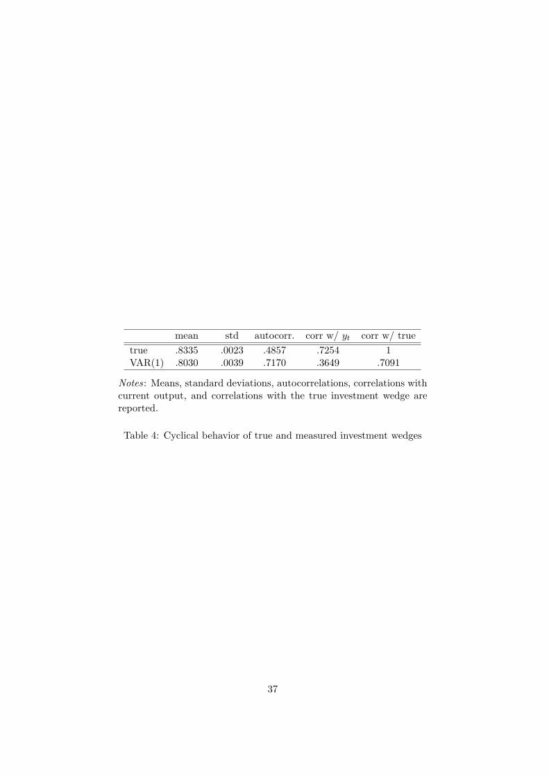
to the true one. Table 4 reports the cyclical behavior of the true and measured investment
wedges: means, standard deviations, autocorrelations, correlations with current output,
and correlations the true current investment wedge. Measured investment wedge is more
volatile and persistent than the true one and the correlation between measured invest-
ment wedge and output is smaller than that between the true and output. However,
differences are small. Therefore, the bias of measured investment is not so large in this
case and measured wedges capture the properties of the true wedges almost correctly17
6 Conclusion
Business cycle accounting rests on the insight that the prototype neoclassical growth
model with time-varying wedges can achieve the same allocation generated by a large
class of frictional models: equivalence results. Equivalence results are shown under
general conditions about the process of wedges while it is often specified to be the first
order vector autoregressive when one applies business cycle accounting to actual data.
In this paper, we characterized the class of frictional models covered by the proto-
type model under the conventional specification and found that it is much smaller than
that believed in previous literature. We also show that even if we employ alternative
specification of the process of wedges, the class covered by the prototype model is not so
large. We also applied BCA to an medium-scale DSGE economy where the equivalence
does not hold and provided an example that measured wedges capture the properties
17Of course, this is just an example. To investigate the statistical properties of the true and measuredinvestment wedges, we have to apply BCA to sufficiently many sample paths. It is our future task.
23

of the true wedges almost correctly even in such an economy. This result tells us that
equivalence results is highly restrictive from the theoretical view, however BCA might
work well empirically since the prototype model is a good approximation of the detailed
model.
24

Appendix A: Proof of Lemma 1
Proof. There exist P that satisfies ΦΨ = PΦ if and only if (24) holds according to the
standard knowledge of linear algebra. In the rest of the proof, we elaborate on sufficiency
and then subsequently, on necessity.
(Sufficiency) Assume that there exists P that satisfies ΦΨ = PΦ. By (20), at period
t + 1,
st+1 = Φ
xt
zt+1
= ΦΨ
xt−1
zt
+ Φ
0
ut+1
= PΦ
xt−1
zt
+ Φ
0
ut+1
= Pst + εt+1, (45)
where
εt+1 ≡ Φ
0
ut+1
. (46)
(Necessity) Assume that there exists P that satisfies CKM’s specification (22). (22) and
(20) imply that
Φ
xt
zt+1
= PΦ
xt−1
zt
+ εt+1. (47)
(21) and (47) imply that
ΦΨ
xt−1
zt
+ Φ
0
ut+1
= PΦ
xt−1
zt
+ εt+1. (48)
25

Since Et[εt+1] = 0 and (48) must hold for any xt−1, zt and ut+1, (46) and
ΦΨ = PΦ (49)
hold.
Appendix B: Proof of Lemma 3
Proof. There exists Λ that satisfies ΛΦ = Θ if and only if (37) holds. In the rest of the
proof, we elaborate on sufficiency and then subsequently, on necessity.
(Sufficiency) Assume that there exists Λ that satisfies ΛΦ = Θ. (19) becomes
ct
it
ℓt
yt
kt
= ΛΦ
xt−1
zt
(50)
= Λ
kt−1
st
. (51)
(Necessity) Assume that (23). By (19) and (28),
(ΛΦ − Θ
) xt−1
zt
= 0. (52)
Therefore, ΛΦ = Θ must hold.
Appendix C: Our Medium-Scale DSGE Model
In this appendix, we present our medium-scale DSGE model used in the investigation of
BCA. Our model has the following properties as in Christiano, Eichenbaum, and Evans
(2005): (i) sticky price with backward price indexation, (ii) sticky wage with backward
26

price indexation, (iii) habit persistence, and (iv) forward-looking Taylor rule. We employ
the Rotemberg adjustment costs for sticky price and wage, not Calvo-pricing. However,
this does not matter since both specification is approximately equivalent in a linearized
economy.18 There are seven independent endogenous and exogenous state variables.19
Therefore, Theorem 1 does not hold and the prototype model cannot cover it.
C.1 Firm
There are competitive final-goods firms and monopolistic competitive intermediate-goods
firms. The production function of final-goods firms is as follows:
yt =[ ∫ 1
0Yt(z)
1−θpθp dz
] θp1−θp
. (53)
The profit maximization of final-goods firms implies demand function of intermediate
goods indexed by z:
Yt(z) =(
Pt(z)Pt
)−θp
yt. (54)
The production function of intermediate-goods firm indexed by z is
Yt(z) = AtKt(z)αLt(z)1−α, (55)
and the productivity At evolves according to
log(At+1) = ρA log(At) + (1 − ρA) log(A) + σAεAt+1. (56)
where A denotes the steady-state of At; σA, the standard deviation of technology shocks;
and εAt+1, i.i.d. shock with standard normal distribution. The cost minimization of
18We employ the log-linear approximation to calculate the aggregate decision rule.19The five endogenous states are consumption c, capital k, nominal interest rate R, inflation rate π, and
wage rate w and the three exogenous states are technology A, government consumption g, and monetarypolicy shock εR
t . However, nominal interest rate is not independent from monetary policy shock becauseof the Taylor rule.
27

intermediate-goods firms implies
rt = α · mct ·Yt(z)Kt(z)
, (57)
wt = (1 − α) · mct ·Yt(z)Lt(z)
. (58)
The Rotemberg adjustment costs which is approximately equivalent to the Calvo-pricing
with price indexation is
ϕp
2
[Pt(z)
Pt−1(z)
/(π1−ξpπ
ξp
t−1
)− 1
]2
yt, (59)
where πt ≡ Pt/Pt−1 is the gross inflation rate. Finally, intermediate-goods firm indexed
by z sets price such that it is a solution to
maxPt(z)
∞∑t=0
βt λt
λ0
(Pt(z)Pt
)1−θp
− mct
(Pt(z)Pt
)−θp
− ϕp
2
[Pt(z)
Pt−1(z)
/(π1−ξpπ
ξp
t−1
)− 1
]2
yt
.
(60)
C.2 Households
The utility function with habit persistence of household indexed by i is
U =∞∑
t=0
βt
[log
(ct(i) − bct−1(i)
)− ψℓ
ℓt(i)σℓ+1
σℓ + 1
], (61)
where b > 0. The evolution of capital stock is
kt(i) = (1 − δ)kt−1(i) + xt(i). (62)
Households have differentiated labor as endowment and they have a power to offer nom-
inal wage. The labor demand is
ℓt(i) =(
Wt(i)Wt
)−θw
Lt, (63)
28

where Wt denotes nominal wage rate. The Rotemberg adjustment costs of nominal wage
which is approximately equivalent to the Calvo-pricing with price indexation is
ϕw
2
[Wt(i)
Wt−1(i)
/(π1−ξwπξw
t−1
)− 1
]2 Wt
Ptℓt. (64)
Finally, the budget constraint is
ct(i) + xt(i) +Bt(i)Pt
= Rt−1Bt−1(i)
Pt+ rtkt−1(i)
+Wt(i)
Ptℓt(i)
1 − ϕw
2
[Wt(i)
Wt−1(i)
/(π1−ξwπξw
t−1
)− 1
]2− Tt + Ωt. (65)
C.3 Policy
The government consumption gt is AR(1):
log(gt+1) = ρg log(gt) + (1 − ρg) log(g) + σgεgt+1, (66)
where g denotes the steady-state of gt; σg, standard deviation of fiscal policy shock; and
εgt+1, i.i.d. shock with standard normal distribution. The monetary authority follows the
forward looking Taylor rule:
Rt = ρRRt−1 + (1 − ρR)[ρπEt
πt+1
+ ρyyt
]+ σRεR
t , (67)
where variables with the hatˆdenotes the log-deviations from the steady-state.
C.4 Resource constraint
The resource constraint is
ct + xt + gt = yt
1 − ϕp
2
[πt
/(π1−ξpπ
ξp
t−1
)− 1
]2− ϕw
2
[πw,t
/(π1−ξwπξw
t−1
)− 1
]2 Wt
Ptℓt, (68)
where πw,t = Wt/Wt−1.
29
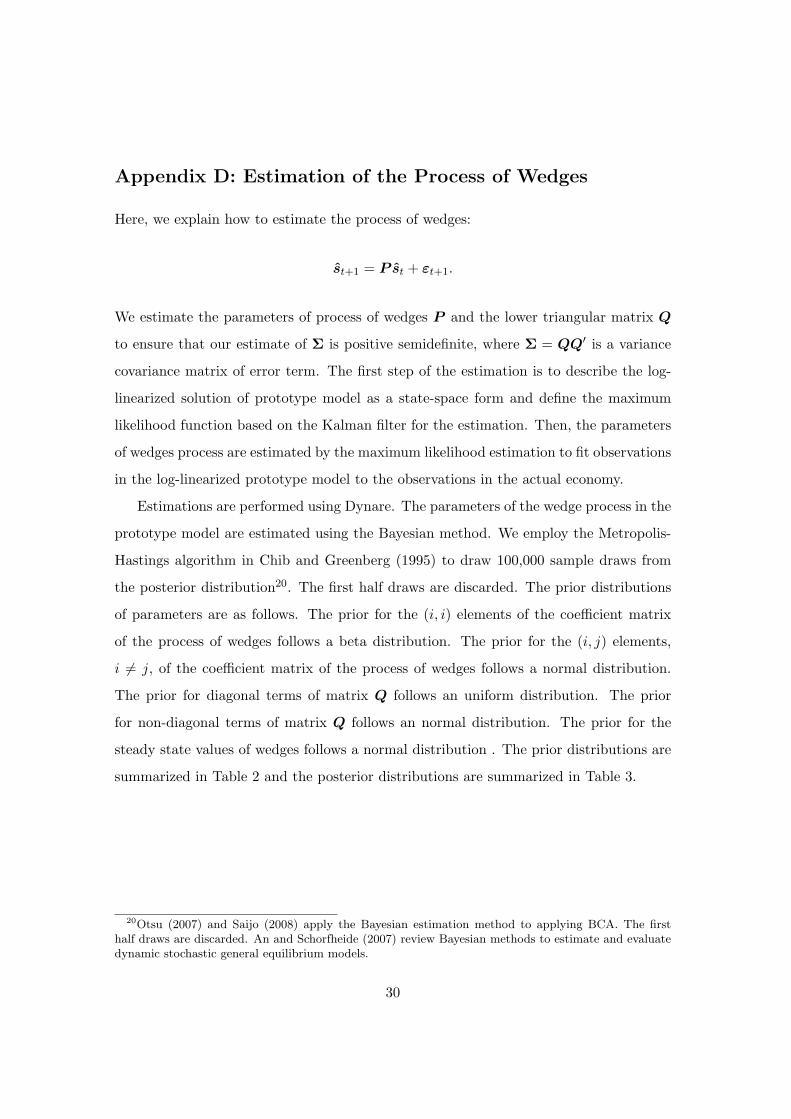
Appendix D: Estimation of the Process of Wedges
Here, we explain how to estimate the process of wedges:
st+1 = P st + εt+1.
We estimate the parameters of process of wedges P and the lower triangular matrix Q
to ensure that our estimate of Σ is positive semidefinite, where Σ = QQ′ is a variance
covariance matrix of error term. The first step of the estimation is to describe the log-
linearized solution of prototype model as a state-space form and define the maximum
likelihood function based on the Kalman filter for the estimation. Then, the parameters
of wedges process are estimated by the maximum likelihood estimation to fit observations
in the log-linearized prototype model to the observations in the actual economy.
Estimations are performed using Dynare. The parameters of the wedge process in the
prototype model are estimated using the Bayesian method. We employ the Metropolis-
Hastings algorithm in Chib and Greenberg (1995) to draw 100,000 sample draws from
the posterior distribution20. The first half draws are discarded. The prior distributions
of parameters are as follows. The prior for the (i, i) elements of the coefficient matrix
of the process of wedges follows a beta distribution. The prior for the (i, j) elements,
i = j, of the coefficient matrix of the process of wedges follows a normal distribution.
The prior for diagonal terms of matrix Q follows an uniform distribution. The prior
for non-diagonal terms of matrix Q follows an normal distribution. The prior for the
steady state values of wedges follows a normal distribution . The prior distributions are
summarized in Table 2 and the posterior distributions are summarized in Table 3.
20Otsu (2007) and Saijo (2008) apply the Bayesian estimation method to applying BCA. The firsthalf draws are discarded. An and Schorfheide (2007) review Bayesian methods to estimate and evaluatedynamic stochastic general equilibrium models.
30
References
[1] An, S. and F. Schorfheide (2007): “Bayesian Analysis of DSGE Models,” Econo-
metric Reviews, 26, 113–172.
[2] Baurle, G. and D. Burren (2007): “A Note on Business Cycle Accounting,”
University of Bern, Discussion Paper 07-05.
[3] Chari, V. V., P. J. Kehoe, and E. R. McGrattan (2002): “Accounting for the
Great Depression,” American Economic Review, 92, 22–27.
[4] ——— (2007a): “Business Cycle Accounting,” Econometrica, 75, 781–836.
[5] ——— (2007b): “Comparing Alternative Representations and Alternative Method-
ologies in Business Cycle Accounting,” Federal Reserve Bank of Minneapolis Staff
Report 384.
[6] Chib, S., and E. Greenberg (1995): “Understanding the Metropolis-Hastings
Algorithm,” The American Statistician, 49, 327–335.
[7] Christiano, L. J. and J. M. Davis (2006): “Two Flaws in Business Cycle Ac-
counting,” Federal Reserve Bank of Chicago Working Paper, 2006-10.
[8] Christiano, L. J., M. Eichembaum, and C. Evans (2005): “Nominal Rigidi-
ties and the Dynamic Effects of a Shock to Monetary Policy,” Journal of Political
Economy 113, 1–45.
[9] Christiano, L. J., M. Eichembaum, and R. Vigfusson (2006): “Assessing
Structural VARs,” in NBER Macroeconomics Annual 2006, ed. by D. Acemoglu,
K. Rogoff and M. Woodford. Cambridge, MA: MIT Press.
[10] Fernanandez-Villaverde, J., J. F. Rubio-Ramırez, T. J. Sargent, and M.
W. Watson (2007): “ABCs (and Ds) of Understanding VARs,” American Economic
Review, 97, 1021–1026.
31
[11] Otsu, K. (2007): “A Neoclassical Analysis of the Asian Crisis: Business Cycle
Accounting of a Small Open Economy,” IMES Discussion Paper Series 07-E-16, Bank
of Japan.
[12] Ravenna, F. (2007): “Vector Autoregressions and Reduced Form Representations
of DSGE Models,” Journal of Monetary Economics, 54 , 2048–2064.
[13] Saijo, H. (2008): “The Japanese Depression in the Interwar Period: A General
Equilibrium Analysis,” forthcoming The B.E. Journal of Macroeconomics.
[14] Uhlig, H. (1999): “A Toolkit for Analyzing Nonlinear Dynamic Stochastic Mod-
els Easily,” in Computational Methods for the Study of Dynamic Economies ed. by
Marimon, R., and A. Scott. Oxford: Oxford University Press.
32

Figure 1: True and measured investment wedges
20 40 60 80 100 120 140 160 180 200
0.82
0.825
0.83
0.835
0.84
True
VAR(1)
Notes: The red solid line is the true wedge generated by the extended detailedmodel. The blue line with x-mark is the measured wedge by the prototypemodel with the VAR(1) specification of wedges.
33

parameter symbol value
discount factor of households β .99Frish elasticity of labor substitution σℓ 1habit persistence b .63steady-state labor supply ℓ .3depreciation rate of capital δ .025Rotemberg adjustment cost of price ϕp 30Rotemberg adjustment cost of wage ϕw 30indexation of price ξp 1indexation of wage ξw 1persistence of technology level ρA .95steady-state technology level A 1standard deviation of technology shock σA .01/4persistence of government consumption ρg .95standard deviation of g shock σg .01/4steady-state ratio of government consumption g/y .1steady-state gross inflation π 1steady-state markup of price θp
θp−1 1.2steady-state markup of wage θw
θw−1 1.2persistence of nominal interest rate ρR .8weight of inflation in Taylor rule ρπ 2weight of output in Taylor rule ρy .2standard deviation of monetary policy shock σR .01/4
Table 1: Parameter values of our medium-scale DSGE model
34

Name Domain Prior density Parameter (1) Parameter (2)parameters
P (1, 1) [0,1) Beta .8 .1P (2, 2) [0,1) Beta .8 .1P (3, 3) [0,1) Beta .8 .1P (4, 4) [0,1) Beta .8 .1P (1, 2) R Normal 0 10P (1, 3) R Normal 0 10P (1, 4) R Normal 0 10P (2, 1) R Normal 0 10P (2, 3) R Normal 0 10P (2, 4) R Normal 0 10P (3, 1) R Normal 0 10P (3, 2) R Normal 0 10P (3, 4) R Normal 0 10P (4, 1) R Normal 0 10P (4, 2) R Normal 0 10P (4, 3) R Normal 0 10log(A) R Normal 0 .0069
log(1 − τℓ) R Normal -.082 .1496log
(1
1−τx
)R Normal .189 .0027
log(g) R Normal -2.298 .0078
standard deviations of shocksεA R+ Uniform 0 .2εℓ R+ Uniform 0 .2εx R+ Uniform 0 .2εg R+ Uniform 0 .2
correlations of shocks(εA, εℓ) [-1,1] Normal 0 .3(εA, εx) [-1,1] Normal 0 .3(εA, εg) [-1,1] Normal 0 .3(εℓ, εx) [-1,1] Normal 0 .3(εℓ, εg) [-1,1] Normal 0 .3(εx, εg) [-1,1] Normal 0 .3
Notes: Parameter (1) and (2) list the means and the standard deviations for beta andnormal distributions and the upper and lower bounds of the support for the uniformdistributions. P (i, j) is the (i, j) component of P and ε ≡ [εA, εℓ, εx, εg]′ denotes theerror term.
Table 2: Prior distributions of the prototype model with the VAR(1) specification ofwedges
35

Name Posterior means 90 % confidence intervalsparameters
P (1, 1) .9137 [.9106 , .9149]P (2, 2) .205 [.2004 , .2103]P (3, 3) .7448 [.7448 , .7472]P (4, 4) .9299 [.9239 , .9386]P (1, 2) -.0033 [-.0035 , -.0027]P (1, 3) -.1024 [-.1027 , -.1017]P (1, 4) -.0014 [-.0044 , -.0003]P (2, 1) 6.8071 [6.813 , 6.8196]P (2, 3) 17.859 [17.8471, 17.8576]P (2, 4) -2.5094 [-2.5229, -2.4901]P (3, 1) -.0881 [-.0881 , -.0881]P (3, 2) -.0019 [-.0019 , -.0018]P (3, 4) .0552 [.0548 , .0552]P (4, 1) .007 [.0072 , .0075]P (4, 2) .0016 [.0015 , .0017]P (4, 3) .0391 [.0391 , .0393]log(A) .0036 [.0036, .0037]
log(1 − τℓ) -.094 [-.0942, -.094]log
(1
1−τx
).1833 [.1833, .1833]
log(g) -2.2988 [-2.2988, -2.2988]
standard deviations of shocksεA .0027 [.0027, .0029]εℓ .1263 [.1182, .1338]εx .0033 [.003, .0035]εg .0026 [.0027, .0027]
correlations of shocks(εA, εℓ) -.0728 [-.0849 ,-.0632](εA, εx) -.2222 [-.2341, -.207](εA, εg) -.0833 [-.0891, -.0413](εℓ, εx) -.9491 [-.9493, -.9488](εℓ, εg) .1512 [.153, .1812](εx, εg) -.0979 [-.1391, -.0922]
Notes: P (i, j) is the (i, j) component of P and ε ≡ [εA, εℓ, εx, εg]′ denotes the errorterm.
Table 3: Posterior means and confidence intervals of the prototype model with theVAR(1) specification of wedges
36
mean std autocorr. corr w/ yt corr w/ truetrue .8335 .0023 .4857 .7254 1VAR(1) .8030 .0039 .7170 .3649 .7091
Notes: Means, standard deviations, autocorrelations, correlations withcurrent output, and correlations with the true investment wedge arereported.
Table 4: Cyclical behavior of true and measured investment wedges
37