On distances between point patterns and their applications

Jorge Mateu∗, Frederic P Schoenberg†, and David M Diez‡

Abstract

Various classes of distance metrics between point patterns are outlined, and their

uses and pros and cons are discussed. Examples include spike-time distance and its

variants, proposed by Victor and Purpura (1997), as well as cluster-based distances

and distances based on classical statistical summaries of point patterns, such as the K-

function or LISA functions. Applications to the summary and description of collections

of repeated realizations of a point process via prototypes or multidimensional scaling

are explored.

Keywords: K-function, LISA functions, point processes, Poisson processes, proto-

types, spike-time distance

1 Introduction

A point pattern is a collection of points falling in some space. A random point pattern, that

is, a process which assigns different likelihoods to different point patterns, is called a point

process. Point process data arise in a wide variety of applications, including epidemiology,

ecology, forestry, mining, hydrology, astronomy, ecology, and meteorology.

∗Department of Mathematics, University Jaume I, E-12071 Castellon, Spain. mateu@mat.uji.es†Department of Statistics, UCLA, 8125 Math-Sciences, Los Angeles, CA 90095, USA.

frederic@stat.ucla.edu‡Department of Statistics, UCLA, 8125 Math-Sciences, Los Angeles, CA 90095, USA.

david.m.diez@gmail.com.

1

Point processes evolved naturally from renewal theory and the statistical analysis of

life tables dating back to the 17th century, and in the earliest applications, each point

represented the occurrence time of an event, such as death or incidence of disease; see Daley

and Vere-Jones (2003) for a review and a thorough treatment of point processes. In the

mid-20th century, interest spanned to spatial point processes, where each point represented

the location of some object or event, such as a tree or sighting of a species. Models

for spatial point processes (see e.g. Cressie (1993)) grew quite intricate, and among the

names associated with these models are some of the key names in the history of statistics,

including Jersey Neyman and David Cox. Today, much attention is paid to space-time

point processes, where each point represents the time and location of an event, such as the

origination of an earthquake or wildfire, a lightning strike, or an incidence of a particular

disease.

Note that point processes are intimately related to time series. As explained in Schoen-

berg (2011), some data sets that are traditionally viewed as realizations of point processes

could in principle also be regarded as time series, and vice versa. For instance, a sequence

of earthquake origin times is typically viewed as a temporal point process, though one

could also store such a sequence as a time series consisting of zeros and ones, with the

ones representing earthquakes. The main difference is that for a point process, the points

can occur at any times in a continuum, whereas for time series, the time intervals are

discretized. In addition, if the points are sufficiently sparse, one can see that it may be far

more practical to store and analyze the data as a point process, rather than deal with a

long list containing mostly zeros.

By the mid 1990s, models for spatial-temporal point processes had become plentiful

and often quite intricate. Around this time, a wealth of neuronal spike train data began

to become available to neuroscientists. Unlike data from seismology or epidemiology, for

2

instance, where the events were naturally seen as one long instance of a point process, the

neuronal data typically consisted of many repeated observations of a point process. For

instance, one might observe the times of firings of neurons in a particular part of the brain

in the instant immediately following a stimulus, for many different subjects, some of whom

have a disease and some of whom do not. The analysis of this type of data required some

slightly different methods.

In order to classify neuronal spike trains into clusters or to differentiate between dis-

eased and healthy patients based on their neuronal firing patterns, methods were sought

which would require the definition of a distance between two point patterns. The seminal

work of Victor and Purpura (1997) proposed several distance metrics, including spike-time

distance, which the authors used for describing neuronal spike trains. The list of distances

in Victor and Purpura (1997) is far from exhaustive, however, and certain alternative types

of distances are more useful for clustered or inhomogeneous point processes or for point

processes in high-dimensional spaces.

The purpose of this article is to outline several types of distances between two point

patterns, X and Y , each observed on the same metric space S. We also discuss some ex-

amples and applications of the proposed distance metrics to cluster analysis and prototype

determination.

The paper is outlined as follows. In Section 2, we discuss spike-time distance and

its variants which involve matching individual points of X to corresponding points in Y .

Section 3 describes distances that might be especially useful for clustered point processes.

Distances based on classical functional or scalar descriptors of point processes, including

estimators of first and second moments of the processes, or classical test statistics based on

these moments, are described in Sections 4 and 5. Applications to summaries of collections

of independent realizations of a point process via prototypes or multidimensional scaling

3

are given in Section 6.

2 Pointwise distances

One family of distances is characterized by a raw transformation of one pattern X into

another pattern Y by actions on individual points. Individual points in X are moved so

that the resulting layout resembles Y .

The spike-time distance metric developed by Victor and Purpura (1997) is one popu-

lar distance metric that has been applied to neuronal, earthquake, and wildfire data (Victor

and Purpura, 1997; Tranbarger and Schoenberg, 2010; Schoenberg and Tranbarger, 2008;

Diez et al., 2010a; Nichols et al., 2010). Techniques for computing this distance metric

were only recently extended to multiple dimensions (Diez et al., 2010a,b). The distance is

defined as the minimum cost associated with the transformation of one point pattern X

into a pattern Y by deleting, adding, and moving points. The left panel of Fig. 1 represents

a transformation of X into Y via actions on individual points of X. Those points in X not

moved are deleted from X, and those points in Y to which no point in X corresponds are

added to X. If we describe such a transformation as T , then the cost associated with T is

C(T |X,Y ) = pd|Xdelete|+ pa|Yadd|+∑

x∈Xmove

pmdx (1)

where pa, pd, and pm are penalty parameters, Xdelete, Yadd, and Xmove are subsets of X and

Y that are deleted, added, and moved, respectively, dx is the distance a point x in Xmove

is moved, and |S| represents the number of points in a set S. The spike-time distance,

ds(X,Y ), is defined as the infimum of equation (1) over all such possible transformations

T . The transformation shown in the left panel of Fig. 1 is the transformation minimizing

(1) for a particular set of parameters. Victor and Purpura (1997) showed that spike-

4

time distance is a well-defined distance metric, and they also considered other closely

related distances. Spike-time distance in single or multiple dimensions may be computed

using the free R statistical software via the stDist function in the ppMeasures package

(R Development Core Team, 2010; Diez et al., 2010b). The C code forming the base of

the package is available through the package page on the R Project website, and a brief

introduction to stDist function is provided in the Appendix. A spike analysis toolkit for

single-dimensional analyses was also made available for MATLAB and Octave (Goldberg

et al., 2009).

Another useful distance function that is also defined in terms of such transformations

of X into Y is the nearest-point distance, where each point x in X is moved to its

nearest neighbor in Y ; call this nearest point yx. Unlike spike-time distance, nearest-point

distances are computed without allowing the addition or deletion of points. The nearest-

point distance is defined simply as

dn(X,Y ) =∑x∈X||x− yx||

where || · || may represent Euclidean distance for point patterns in Rk, or some other

distance metric for point patterns in a more general metric space. The measure dn is

useful in facility placement. For instance, if points in X represent consumers and points in

Y represent facilities, then dn characterizes the total cost for all consumers to visit their

closest facility. Note that for two distinct points x, x′ in X, we may have yx ≡ yx′ , and that

in general, dn(X,Y ) 6= dn(Y,X), so that dn is not formally a distance metric. However,

the sum of these two distances forms a symmetric nearest-point distance metric:

dN (X,Y ) = dn(X,Y ) + dn(Y,X).

5

1

2

3

4

5

6

789

12

3

4

5

6

7

8

9

XY

Y[1:nx]

1

2

3

4

5

6

789

12

3

4

5

6

7

8

9

XY

Figure 1: Spike-time distance (left) and nearest-point distance for moving X to Y (right).

3 Distances for cluster processes

When a point process is highly clustered, metrics such as spike-time distance tend to

yield prototypes that do not reflect a typical sample point pattern. Clustered processes

thus require a separate family of distances where movements of collections of points are

permitted. For example, consider the following metric, called cluster distance. Let T

represent a transformation of X into Y that involves sequentially moving collections of

points in X. Thus, T is itself a sequence of transformations, ti, where each ti moves a

subset Xi of points by a vector zi (see the first two panels of Fig. 2). Then the cost

associated with T is defined as

pd|Xdelete|+ pa|Yadd|+∑i

pm|Xi|q||zi|| (2)

where q is a parameter in [0, 1). The cluster distance, dc(X,Y ), is the infinum cost over all

such transformations, T . The further each cluster must be moved (the larger zi is), and

the more points that must be moved in order to match X up with Y (the larger |Xi| is),

the larger the cluster distance between X and Y .

6

A similar type of distance for clustered point processes is defined by first aligning

clusters in X with clusters in Y and subsequently applying simple spike-time distance.

For instance, let {Rj} represent a set of disjoint and concave regions of the space that

contain all the points of X. One may translate all of the points in a given region by

some fixed vector and repeat for each region, assigning a cost of pc per unit distance to

each translated region, and then spike-time distance may be applied after these regions

are moved. This declustered spike-time distance is defined as the minimum cost over

all such transformations and choices of {Rj}. An illustration is given in the right panel of

Fig. 2.

XY

allpoints

in X

Cluster 1

x1[,

2]

XY

singleclustermoved

Cluster 2

x[,2

]

XY

Declustering

Figure 2: The first two steps in the cluster distance are shown in the left and center panels.The right panel represents the process of removing the clustering characteristics prior toapplying spike-time distance.

A drawback of both cluster distance and declustered spike-time distance is that methods

for their efficient computation appear to be unavailable presently, and searching over all

possible translations of all possible subsets of points in X is extremely computationally

burdensome. An advantage of cluster distance is that the clusters Xi and their associated

translation vectors, zi, may have physical meaning and be of direct interest. For instance,

a subset of point pattern X is nearly equivalent to a subset of point pattern Y in the

case of a temporal delay in response to stimuli, in the case where the points are observed

in time, and in the purely spatial case, the points in X or Y may be translated due

7

to physical deformation or may require spatial translation due to mis-calibration of the

recording instruments.

4 Distances based on functional summaries

4.1 Model-based distances

One way to construct a statistical model (in any field of statistics) is to write down its

probability density. One advantages of doing this is that the functional form of the density

reflects its probabilistic properties, and the terms or factors in the density often have an

interpretation as components of the model. This approach is useful provided the density

can be written down, and provided the density is tractable. Probability densities for point

processes behave much like probability densities in more familiar contexts. Spatial point

process models that are constructed by writing down their probability densities are of

interest to the statistical community, and a widely known and used such class of models

is called Gibbs processes. To construct spatial point processes which exhibit interpoint

interaction (stochastic dependence between points), we need to introduce terms in the

density that depend on more than one point.

Each point process model is specified in terms of its conditional intensity rather than

its likelihood. This turns out to be an intuitively appealing way to formulate point pro-

cess models, as well as being necessary for technical reasons. For spatial point processes,

the lack of a natural ordering in two-dimensional space implies that there is no natural

generalization of the conditional intensity of a temporal or spatiotemporal process given

the past or history up to time t. Instead, the appropriate counterpart for a spatial point

process is the Papangelou conditional intensity (Daley and Vere-Jones (2003)), say λ(u,X),

which conditions on the outcome of the process at all spatial locations other than u. Infor-

8

mally, λ(u,X)du gives the conditional probability of finding a point of the process inside

an infinitesimal neighborhood of the location u, given the complete point pattern at all

other locations. The Papangelou conditional intensity of a finite point process uniquely

determines its probability density and vice-versa.

Given specific models for the point processes giving rise to the point patterns X and

Y , one may define the distance between X and Y in terms of the differences between char-

acteristics of these models. For instance, if the point processes X and Y are characterized

by their conditional intensities λX(x) and λY (x), respectively, then one measure of the

difference in these point process models is the integral of the squared difference of the two

conditional intensities over the observation region S:

dMB(X,Y ) =

∫S

(λX(x)− λY (x))2dx. (3)

This is illustrated in the left panel of Fig. 3, where the intensity functions have been

estimated based on the data shown at the top of the panel. These methods readily extend

to a variety of other summaries, such as the integrated squared difference between the

overall mean, or second moment measure, or higher moments or cumulants of the processes.

Of course, the conditional intensities in (3) may be replaced by their expected values, their

overall intensities, or in the spatial point process setting, by the Papangelou intensities (see

e.g. Daley and Vere-Jones (2003)).

4.2 Distances based on classical functional statistical summaries

Differences in point process behavior can also be characterized by comparing classical

summary measures of the first or second moments for each of the point patterns. For

instance, given two point patterns X and Y , one could imagine looking at an estimate of

the overall intensity of X, e.g. a kernel estimate, and a similar estimate of the intensity

9

of Y . Alternatively, if each of the point patterns is one-dimensional, then one could look

at the empirical cumulative distribution function for each point pattern as a statistical

summary of the realization.

In his influential paper Ripley (1977) developed an exploratory analysis of interpoint

interaction, assuming that the data are spatially homogeneous. A useful summary statistic

is the nonparametric estimator of Ripley’s K-function, essentially a renormalized empirical

distribution of the pairwise distances between observed points. More pragmatically, for a

stationary point process with intensity (mean number of points per unit area) λ, λK(r)

gives the expected number of other points of the process within a distance r of a typical

point of the process.

Thus, a further alternative would be to take the estimated K-function or its derivative,

the estimated reduced 2nd moment measure, for each pattern, and examine the difference.

As an illustration, one could compare the integrated squared difference between estimates

of Ripley’s K-function for two point patterns:

∫(K1(r)− K2(r))

2dr (4)

This distance is illustrated in the right panel of Fig. 3.

First and second order measures represent a valuable description of a spatial point

process but do not generally uniquely characterize a point process. Additional important

summary descriptions are given by distance methods based on measures of some distances

between points. The nearest neighbor distance D may be defined as the distance from a

point of the pattern to the closest of the other points in the same pattern. The empty

space distance F is the distance from an arbitrary fixed location to the nearest point of

the pattern. For a given point pattern, a set of distances (nearest neighbor or empty space

distance) can be summarized by means of their corresponding distribution functions. Let

10

position

inte

nsity

est

imat

e

−1 0 1 2 3 4 5

0

5

10YX

λX

λY

0

11

Cum

ulat

ive

Cos

t

R

K fu

nctio

n

0

8

0 1 2 3 4 5

0

5

10

15

20

Cum

ulat

ive

Cos

t

Figure 3: Left: A comparison of two intensity models using Equation (3). In this illus-tration, the intensities λX and λY are estimated by kernel smoothing the points in X andY , respectively. Right: an example using Equation (4) to characterize the difference inclustering behavior of two patterns using Ripley’s K function.

G(r) denote the nearest-neighbor distribution function, and F (r) the corresponding first

contact distribution function or empty space function. These distribution functions may

be estimated from the observed point patterns X and Y using conventional methods. For

example, if di define the distance from each of m points in a regular lattice arrangement

to the nearest event, then F (r) = m−1∑I(di ≤ r), where I(·) is the indicator function.

Similarly, if ei is the distance from each of n events of the point pattern to its nearest

neighbour, then G(r) = n−1∑I(ei ≤ r).

In practice, each point pattern is typically observed in a bounded region S, and without

precautions, these boundaries can lead to biased estimates. This problem is known in

the context of spatial statistics as edge-effects. Different edge-corrected estimators of the

functions F and G have been proposed (see e.g. Cressie (1993)). There is a clear analogy

with censoring in the context of survival analysis Baddeley and Gill (1997). The different

distances observed within a single point pattern are really censored distances. Let di denote

the observed distance from the ith point of the point pattern to its nearest neighbor within

11

the sampling window, W , and ci its distance to the complement of the sampling window

W . If ci < di the real nearest neighbor could be outside the window and, in this case,

the real and unknown nearest neighbor distance di fulfills di > ci, and the observation is

censored. A similar comment applies to empty space distances. In both cases the censoring

distance is the distance from the sampling point to the frame window.

Given a statistical summary such as the estimated F or G-function of the point pro-

cesses, the dissimilarity between point processes X and Y can be defined as the distance

between the corresponding estimated functional summaries. For instance, let FX and FY

be the corresponding estimated empty-space distribution functions for X and Y . The

dissimilarity between X and Y can thus be defined as

D(X,Y ) = d(FX , FY ) (5)

where d stands for a metric between the functions. For instance, one may use the L2 metric

D2F (X,Y ) =

∫ r0

0(FX(r)− FY (r))2dr (6)

or the L∞ metric:

D∞F (X,Y ) = supr‖FX(r)− FY (r)‖ (7)

By replacing the empty-space distribution function with the nearest-neighbor distribu-

tion functionG orK-functionK, one can similarly defineD2G(X,Y ), D∞G (X,Y ), D2

K(X,Y ),

and D∞K (X,Y ), respectively. Note that sampling variability in estimates of K(r) tend to

increase with r and this can have a great influence on the value of the dissimilarity measure.

This suggests the use of the L-function proposed by Besag (1977), a variance stabilized

version of the K-function.

12

4.3 Distances based on LISA functions

When estimated from point process data, the empirical product density function provides

a description of the density of inter-event distances in an observed point pattern. For

instance, high values for small distances are indicative of an overabundance of short inter-

event distances (this is a typical situation for cluster processes, where data tend to form

groups). Conversely, if short inter-event distances are rare, this will indicate that an

inhibitory structure is present, and points tend to separate from each other.

Both the K-function and the product density function provide a global measure of

the covariance structure by summing over the contributions from each event observed in

the process. Now we consider individual contributions to the estimated function that are

analogous to the local statistics described by Anselin (1995) and called local indicators

of spatial association (LISA). An individual LISA product density function for a given

point pattern X, lXi (·), should reveal the extent of the contribution of the i− th event to

the global estimate of the product density lX(·), and may provide a further description

of structure in the data (e.g., determining events with similar local structure through

dissimilarity measures of the individual LISA functions). A product density LISA function

can be constructed in the same manner as the global estimate (Cressie and Collins, 2001).

Given point patterns X = {x1, x2, . . . , xn} and Y = {y1, y2, . . . , ym}, one may calculate

the set of LISA functions for each pattern corresponding to any individual or spatial loca-

tion. Denote both sets by {lXi (r), i = 1, . . . , n} and {lYj (r), j = 1, . . . ,m}. Then one may

derive several possibilities for distances between X and Y , such as

13

(a) Define

AXL = 1/(n× (n− 1))

∑i

∑j

d(lXi (r), lXj (r))

= 1/(n× (n− 1))∑i

∑j

∫(lXi (r)− lXj (r))2dr (8)

as the average of all pairwise distances between LISA functions of points in X. Define the

same average for points in Y , say, AYL . Then, a similarity or dissimilarity measure is given

by

dL(X,Y ) = AXL −AY

L . (9)

(b) Define the average LISA function coming from the set of LISA functions for points

in X and Y . Denote them by lX(r) and lY (r). Note that lX(r) is a function itself. Then

one may define a distance measure via

dl(X,Y ) = d(lX(r), lY (r)) =

∫(lX(r)− lY (r))2dr. (10)

4.4 The proximity function of an individual to a population based on

LISA distances

Let dX(i, j) = d(lXi (r), lXj (r)), i, j = 1, . . . , n the set of pairwise distances between LISA

functions for points in X. Following Cuadras et al. (1997), define the geometric variability

for pattern X as

VdX =1

2n2

∑i,j

d2X(i, j) (11)

14

Then the proximity function for the i− th point in X i = 1, . . . , n is given by

Φ2X(i) =

1

n

n∑j=1

d2X(i, j)− VdX (12)

Hence the value of the associated proximity-based density function for the i− th point in

X for i = 1, . . . , n is given by

fX(i) = exp{−1

2Φ2X(i)} (13)

One may proceed similarly with pattern Y defining VdY , Φ2Y (j) and fY (j) for j =

1, . . . ,m.

Finally, the distance between patterns X and Y may be defined as a measure of simi-

larity/dissimilarity between the densities fX and fY , as dP (X,Y ) = d(fX , fY ).

5 Distances based on numerical test statistics

One could alternatively compare point processes X and Y based on single numerical sum-

maries of each point process. For instance, given the same parametric model for the two

processes, one could obtain estimates θX and θY of the parameter vector governing each

of the two processes, given the realizations X and Y , respectively. The distance between

X and Y could then be defined simply as ||θX − θY ||.

A related idea is to describe the similarity between X and Y in terms of a numerical

summary of the degree of clustering or inhomogeneity in each. An example would be a

generalization to the point process context of the log rank test (Mantel and Haenszel, 1959)

or Kolmogorov-Smirnov type statistic (Fleming and Harrington, 1981), where the time or

duration usual in the context of survival analysis is replaced here by the distance observed.

15

For instance, consider the following generalization of the log rank test of Mantel and

Haenszel (1959). In survival analysis, the time instant where an event is observed is

frequently called (observed) failure time. Here this phrase is replaced by (observed) failure

distance, i.e., the distance between a point of the pattern and its nearest neighbor or the

distance between a sampling point and the nearest event of the point pattern, provided

that these distances are smaller than the distances to the boundary of the window. In

order to construct the log rank test, a sequence of 2 × 2 tables is built over the distances

(one for each failure distance, dj), where the risk set at that distance is classified into a

2× 2 table, according to group and event status. Let us present some notations: rj stands

for the size of the risk set in the interval [dj−1, dj) and fj the number of failures. The size

of the risk and failure sets for each group can also be defined. In this way, for the first

group, they are denoted by r1j and f1j respectively. Differences between the observed and

the expected events (conditioning on the margins of the 2× 2 table) on the first group are

added up over distances and squared in order to calculate the numerator of the log rank

statistic:

U =∑j

(f1j − g1j), (14)

where g1j stands for the expected number of failures in the first group, g1j = fj · r1j/rj .

The denominator is the sum of the variances of the number of events on the first group

within each 2× 2 table, which is obtained by using the hyper-geometric distribution:

V ar(U) =∑j

t1j · fj/rj(1− fj/rj)(rj − r1j)/(rj − 1) (15)

The null distribution of U2/V ar(U) is approximately chi-squared with one degree of free-

dom. The log rank test is more sensitive to differences at the right tails of the two survival

distributions and more suitable for detecting departures when hazards are proportional

16

(Lee, 1992). There are cases in which this test is not very effective, and one may use

a Kolmogorov-Smirnov type statistic, i.e. the supremum of appropriately scaled empiri-

cal processes. This test is sensitive to differences that are large at a particular point. A

detailed explanation can be found in Fleming and Harrington (1981).

6 Applying measures to a collection of patterns

Distance measures can be used in the identification of prototypical patterns or with mul-

tidimensional scaling for classification. Each technique is considered in the context of a

collection of patterns that come from either one or many point processes, and an introduc-

tion to referenced R packages is included in the Appendix.

6.1 Prototypical patterns

One application of distance measures is in the construction of a point pattern proto-

type, which is the typical pattern of a collection. Prototypes are useful for identifying the

typical pattern in a collection, much like the median is used to describe the typical obser-

vation in a univariate data set. The prototype has generally been used to construct robust

representations of a collection of patterns using spike-time distance as the distance met-

ric in applications including neuronal spike behavior, earthquake aftershocks, and wildfire

activity in California (Schoenberg and Tranbarger, 2008; Diez et al., 2010a; Nichols et al.,

2010).

The prototype Pd(C) of the collection of patterns C based on the distance measure d is

defined as the pattern that minimizes the following loss function:

argminP∑Xi∈C

αid(P,Xi)

17

where αi is the weight corresponding to point pattern Xi. The weights αi are typically

chosen to be unity unless certain point patterns are deemed more important than others,

or if the point patterns are measured with differential error. Recall that the median and

mean can be defined in a similar way: each is the minimizer of a loss function represented

by the sum of distances, the L1 norm for the median and L2 norm for the mean.

Kernel density and prototype summaries for ten simulated patterns are shown in Fig. 4.

The kernel density is a pooled estimate based on all patterns and is heavily influenced by

pattern 10. The prototype, using spike-time distance, is shown to be resistant to the tenth

pattern and characterizes the typical pattern in the collection.

time

patte

rn n

umbe

r

● ● ● ●

● ● ●

● ● ● ●

●● ● ●

● ● ● ●

● ● ● ●

●● ● ●

● ● ●

● ● ● ●

●● ● ●● ● ● ●●● ●● ●● ●●● ●● ●● ●● ● ●● ●● ●●●● ●●● ●

0 1 2 3 4 5 6 7

123456789

10

0.00.81.6

prototype ●● ●●

Figure 4: Kernel density and prototype summaries for a collection of ten patterns. Eachpattern is represented by a sequence of events at times denoted by circles.

A two-dimensional example of a prototype is shown in Fig. 5. Here the sample collection

contains 10 point patterns, nine of which are realizations of an inhomogeneous Poisson

process with intensity shown in the plot in the first row and first column. Each pattern

is expected to have about 15 points. The last point pattern – row 3, column 1 – is a

realization of a homogeneous Poisson process with an overall intensity of three times that

18

of the original process. Just as in the one-dimensional case, the prototype, shown in the

bottom-right panel, is resistant to a single atypical pattern.

x$xB

0

26

53

●

●

● ●

●

●

●

●

X[[i]]$y[,1]

X[[i

]]$y[

,2]

●

●

●

●

●

●

●

●

●

●

●

●

● ●

●

X[[i]]$y[,1]

X[[i

]]$y[

,2]

●

●

●

●

●

●

●

●

● ●

●

●

●

X[[i]]$y[,1]

●

●

●●

● ●

●

●●

●

●

●

●

●

●

●

●

●

●

X[[i]]$y[,1]

X[[i

]]$y[

,2]

●

●

●

●

●

●

●●

●

●

●

●

●

●●

X[[i]]$y[,1]

X[[i

]]$y[

,2]

●

●

●

●●●

●

●

●

●●

●

● ●

●

●

●

● ●

X[[i]]$y[,1]

X[[i

]]$y[

,2]

●

●●

●

●

●

●

●

●

●

●●

●

●

●

●

●

●

●●

●

●

●

●

●

●

●

●

●

●

●

●

●

●

●●

●

●

●

●

●

●

●

●

● ●

●

●

●

●

●

●

●

●

●

●

●

X[[i

]]$y[

,2]

●

●●

●

●

●

● ●

●

●

●

●

●

● ●

X[[i

]]$y[

,2]

●

●

●

●

●

●●

●

●

●

●

●dim

2

Figure 5: The top-left panel shows an intensity function over the space [0, 1]× [0, 1]. Thesecond panel in the first row represents a legend of the intensity, and the next 9 panelsshow simulations of an inhomogeneous Poisson process based on the intensity, except thebottom-left panel, which is a realization of a homogeneous Poisson process with λ = 42.The prototype of these 9 point patterns, using spike-time distance with parameters chosenby default according to the recommendations in Diez et al. (2010a), is shown in the bottom-right panel.

Tranbarger and Schoenberg (2010) developed techniques for estimating the prototype

in one dimension. This work was extended to multiple dimensions in Diez et al. (2010a);

Diez (2010). Prototype methods are freely available through the ppPrototype function in

the ppMeasures package on CRAN (R Development Core Team, 2010; Diez et al., 2010b).

Many additional examples are included in the package help files.

19

6.2 Multidimensional scaling

Classical multidimensional scaling (MDS) is useful for pattern classification based on a

distance metric. Given a collection of point patterns, C = {X1, ..., Xn}, a distance matrix

D is computed where Di,j = d(Xi, Xj) for some distance measure d. MDS uses this distance

matrix to estimate relative locations of the patterns in the Rk where k is generally selected

by the user. Each pattern is itself represented by a point, and MDS embeds these points

in locations of Rk. The goal of this embedding is to place points representing similar

(dissimilar) patterns close to (far from) each other. To achieve this aim, MDS selects a

location for each pattern such that the resulting Euclidean distances between the patterns,

described by D, approximates the pattern distances D by minimizing the following loss

function:

L(D, D) =∑i 6=j

[Dij − Dij

]2.

See e.g. Venables and Ripley (2002) for additional details on classical MDS and its variants,

such as Kruskal’s MDS and Sammon mapping.

MDS can be useful in both identifying groupings of points – in this case, groups of

patterns – and in classification. If classifications are provided on a training set, then

a distance metric may be applied to compute the distance matrix D. Applying MDS

places the patterns into a new space Rk, where traditional classification techniques may be

applied. The MDS methods are implemented in the R package smacof using the smacofSym

function (de Leeuw and Mair, 2009).

Fig. 6 shows 15 patterns in one-dimensional space. Each pattern arose from a Poisson

process with an overall mean of 12 points per pattern, as described by the figure’s intensities

in the left panel. The right panel of Fig. 6 shows MDS applied to these fifteen patterns

20

using spike-time distance. One sees a grouping of the patterns based on their original

intensity functions.

0 5 10 15

0.0

0.5

1.0

1.5

2.0

time

process 1process 2

time

patte

rn● ● ●●● ●●● ●● ● ●●

●● ● ●● ●●● ●●● ● ●

● ●● ●● ●● ●●●

●●● ●●● ● ●●

● ●● ● ●●● ●● ●

● ● ●● ●● ●● ●● ●● ●●

●● ●● ● ●●● ●●

● ●● ●●● ●● ●● ●●● ●● ●

● ●● ●● ●●●● ●

●●● ●● ●

● ●●● ●●● ●● ● ●●

● ●●● ●●●● ●

● ●●●● ●● ●●● ●●● ● ●

●● ●●●● ●● ●●● ●● ●●● ●● ●● ●

●● ●●● ● ● ●●● ● ●

0 5 10 15pr

oces

s 1

proc

ess

2

●

●

●●

●

MDS, dimension 1

MD

S, d

imen

sion

2

−0.5 0.0 0.5 1.0

−1.

0−

0.5

0.0

0.5

Figure 6: Left: Two Poisson intensities, each with a total intensity of 12. Middle: 15patterns, five from the first Poisson process and ten from a second Poisson process depictedin the left panel. Right: Spike time distance was used as the metric to construct the matrixD, and multidimensional scaling applied to all 15 patterns. The black circles denote thefirst five patterns and the red crosses mark those of the second process.

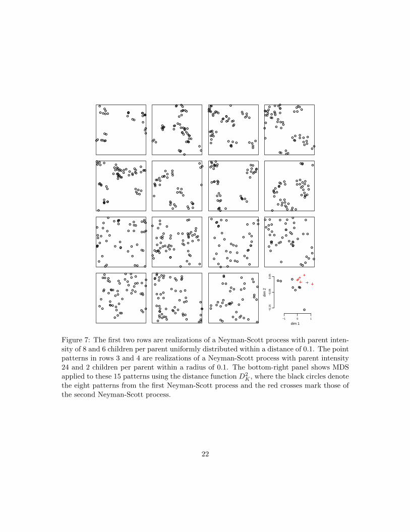
Multidimensional scaling may be applied to any of the distance metrics introduced.

Fig. 7 shows a second example of 15 two-dimensional patterns and their representation

as points in [0, 1] × [0, 1] where the distance D2K was used to construct the dissimilarity

matrix. Each point pattern is a realization of one of two Neyman-Scott processes with

different parameters. Again, one sees that MDS is quite successful at classifying the point

patterns into two groups.

Appendix: Spike-time distance, prototypes, and multidimen-

sional scaling in R

We consider the packages ppMeasures and smacof for the R statistical software. These

packages and the R statistical software are freely available online from the Comprehensive

R Archive Network: r-project.org. The ppMeasures and smacof packages are useful in

21

●

●●

●

●● ●

●

●

●●●

●

●

●

●

●

●

●

●●

●

●●

●●

●●● ●

●

●●

●

●

● ●

●

●

●

●

●

● ●

●●

●●

●

●

●●

●●

●

●●

●●

●

●●●

●●●●

●●

●●

●●

●●

●●●●●●

●

●●

●

●

● ●

●

●

●●

● ●

●●

●

●●

●

●●

●

●●

●●

●

●●

●●

●

● ●●

●

●●●

●

●●

●●●

●

●●●

●●●

●

●●

●●

●

●

●●

●

●

●

●

●

●●

●

●

●

●● ●

●

●

●●

●

●

●●

●● ●

●

●●

●

●●

●●

●●● ●

● ●●

●●

●●

● ●

●●

●●

●

●

●

●●

●

●

●

●●

●●●

●

●

●●

●●

●

●

●●●

●

●●

●●●

●

●

●●●

●

●

●●

●●●●

●

●●

● ●

●

●●●

●

●●

●

●

●

●

●●●

●●●

●

●

●●●

●

●

●

●●

●●●

●

●●

●

● ●

●

●

●●

●

●

●

●●● ●●

●

●

●●

● ●● ●

●

●

●

●●

●

●●●

●●

●

●

●

●

●

●

●

●

● ●●

●●●

●●●●

●

●

● ●●●

●

●

●●● ●●●

●

●

●●

●●

●●

●●●

●● ●

●●

●●

●

●

●

●

● ●●●

●

●

● ●●

●

●

●● ●

●

●

●

● ●

●●● ●

●

●

●

●

●

●

●

●

●

●

●●

●●

● ●

●

●●

● ●

●●

●

●

●●

●●

●●●●

●

●

●

●

●●

●

●

●●

●

●

●

●

●

●

●●

●

●

●●

●

●

●●

●

●

●

●

●●

●

● ●●

● ●●●

●●

●

●

●

●

●

●

●●

●

●

●●

●

●

●

●

●

●

●

●●

●

●

●●

●●

●

●

●●

●●

●●

● ●

●●

● ●

●

●

●●

●

●

●

●●

●●

●

●

●

●

●

●

●

●●

●

●

●

●●

● ●

●

●

●●

●

●

●

●

●●

●

●

●

●

●

●●

●

●

●●

●

●●

●

●●●●

●●●

●

●

●

●

●

●

●●

●

●

●●

●

●

●

●

●●

●

●

●

●

●

●

●

● ●

●

●

●●

●

●

●●

●●

●●

●

● ●● ●

●

●

●

●

●

●

●●

●

●

● ●

●

●

●

●

●

●●

●

●

●

●

●●

●

●

●

●

●●

● ●

●●

●●●●

●

●

●

●

●●

●

●●

●

● ●

●

●

●●

●

●

●●

● ●

●

●

●

●

●●

●

●●●

●

●●

●●

●

●

●●

●●

●●

● ●

●●

●●

●

●

●

● ●●

●

●

●

●

●

●

●

●

●● ●

●

●●●

●

●●

●●

●

●

●

●

● ●●

●

●●

●●

●

●

●

●

●

●●

●●

●●

●

●

●

●

dim 1

dim

2

−1 0 1

−0.

15−

0.05

0.05

Figure 7: The first two rows are realizations of a Neyman-Scott process with parent inten-sity of 8 and 6 children per parent uniformly distributed within a distance of 0.1. The pointpatterns in rows 3 and 4 are realizations of a Neyman-Scott process with parent intensity24 and 2 children per parent within a radius of 0.1. The bottom-right panel shows MDSapplied to these 15 patterns using the distance function D2

K , where the black circles denotethe eight patterns from the first Neyman-Scott process and the red crosses mark those ofthe second Neyman-Scott process.

22

computing spike-time distance, prototypes, and implementing multidimensional scaling.

This introduction uses simulated data, and we assume the user is familiar vectors, matrices,

loops, subsetting techniques, and basic plotting in R. To install the packages using an

internet connection, use the install.packages function, and to load the packages, use

the library function:

> install.packages(c(’ppMeasures’, ’smacof’))

> library(ppMeasures)

> library(smacof)

Spike-time distance is useful in assessing the similarity or dissimilarity in two point

patterns. The stDist function in the ppMeasures package computes spike-time distance

for two patterns. Its required arguments are the two point patterns entered as matrices,

where rows represent points, and a moving penalty that can be a single value or a vector

where the ith entry corresponds to movement in the ith dimension. Additional arguments

include addition and deletion penalties, and other arguments that may be modified to

compute variants of spike-time distance and other function options. Below two patterns are

generated, p1 and p2, using the rgamma function to generate the location of the points. The

distance is computed using a moving penalty of 10 and the default addition and deletion

penalties, which are both 1. A graphic representing how the distance was computed is

generated using the plot method applied to the output of stDist, which is shown in the

left panel of Fig. 8. Points connected by a line represent corresponding points in patterns

1 and 2, and isolated points represent added or deleted points.

> p1 <- cbind(rgamma(20, 2), rgamma(20, 1.8))

> p2 <- cbind(rgamma(20, 2), rgamma(20, 1.8))

> (hold <- stDist(p1, p2, 1))

[1] 19.35158

23

●

●

●

●

●●

●

●

●

●

●

● ●

●

●

●

●●

●●

0 1 2 3 4 5 6

0

1

2

3

4

5

dim 1

dim

2 ●

●

●

●

● ●

●

● ●

●●

●●

●

●

●

●

●

●

●

●

●

pattern 1pattern 2

● ●● ●● ●●●● ● ●●● ●●●● ●●●● ●●●● ● ●●● ● ●● ●●●● ●●● ●●●● ●● ● ●●● ●● ●

● ● ●● ● ● ●●● ●● ●●●● ●● ●●● ●● ●● ●●● ●● ●● ● ●● ●● ●●● ●● ● ●●

● ●●● ●● ●● ● ●● ●● ●●● ●●●● ●● ●●●● ● ●●●● ●● ●●●● ●● ●●● ●●● ●● ●

● ● ●●● ●●● ●●● ●● ●●● ● ●● ●●●● ●● ●●● ●●● ● ●● ●● ● ●● ●● ●● ●●

● ●●● ●●●● ●● ●●● ● ●● ●● ●● ●● ●● ●●●● ●● ● ●● ●●●● ●●● ●●● ●● ●●● ●● ●● ● ●●● ● ●● ●● ●●

●●● ●● ● ●● ● ●●●● ●● ● ●●● ● ●● ● ●● ● ●●● ●●● ● ● ●●● ●●●●● ●●● ● ●● ● ●● ● ●● ●● ●●● ● ●

● ● ●● ● ●● ●● ●●● ●● ● ● ● ●●●●● ●●●● ●● ●●●● ● ●● ● ●● ●● ●● ●● ●● ●● ●● ●●● ●

●● ●● ●● ●● ●● ●●●● ● ●● ●● ●●● ●●●● ●●● ●● ●● ●● ●● ● ●●● ●●●● ● ●● ●● ● ●●● ●

● ●●●● ● ●●● ●● ●●● ●● ●●● ●●● ● ●●● ●●● ●● ●●●●● ●● ●● ●●● ●● ● ● ●● ●● ●● ●●● ●●●● ●● ●● ●●●●

●●● ●●● ●● ● ● ●●●●●● ● ●● ●● ●● ● ●●● ●● ●● ● ● ● ●● ● ●● ●●● ●●●● ●●● ●● ●● ●●●●●●● ●● ●● ● ●● ●●●● ●● ● ●

●● ●● ● ●● ● ●● ●●● ●● ●● ● ●● ●● ●● ● ●● ●●●●● ●● ● ●●●●●● ●● ● ●●● ●● ●●

●●●● ● ●● ●● ● ●● ●● ● ● ●●● ●● ●● ●●●● ●● ●●● ●● ●●● ● ●● ●●● ●●●● ●●● ●●● ●●● ●● ●●● ●● ●● ●● ●● ●●● ●● ● ●●● ●●●

●● ●● ●● ●●● ● ●● ●●●● ●●●● ● ●●● ●●● ● ●● ●● ●●● ● ●●●●●●●● ●● ● ●●●●● ●● ●● ● ●● ● ●●● ●●

● ●●●● ●● ●● ●●● ● ●●●●● ●● ●●●● ● ●● ●●●● ●●● ● ● ● ●●●●●●●● ● ●● ●● ●●● ● ● ●● ●●●●● ●●●●●●● ●● ●● ●

● ● ●● ●● ●●● ● ●●● ● ●●● ●●● ●● ●●● ●● ● ●●● ● ●● ●● ●● ● ● ●●● ●●● ●●●● ●●●●● ●● ●●● ●● ●● ● ● ●●● ●●●

●● ●● ● ●●● ● ●● ●● ●●●● ●●● ●●● ● ●● ●●● ● ●●● ●●● ●● ●●● ●● ●● ● ●●●● ●● ● ●●

●● ●●●● ●● ●● ●● ●●●● ●● ●● ● ●●●● ●● ●● ● ●●●● ●● ● ●● ● ● ●●● ●●● ●● ● ●● ●● ● ● ● ● ●●●● ● ●●

● ● ●● ●●● ● ●● ●● ●●● ●● ●●● ● ●●●● ●● ●● ●● ● ● ●●● ●● ●●● ●●●● ●●

●●● ●●● ●● ●●● ●●● ● ●●●● ●● ●●● ●●● ●

● ● ●●●● ●●● ●●●●●●●● ●●●● ●● ●●●● ● ●

●●● ●● ●● ●●●● ● ● ●●● ● ● ●●● ●● ● ●●●● ●●

●● ●● ●● ●● ●●●● ●● ●● ●●●● ●● ●● ●●●● ● ●● ●●●● ●●● ● ●● ●●●●

●●●● ●● ●● ●● ●●● ●●●● ●● ●● ●●●● ●● ●●● ●● ●

●● ● ●●● ●● ●●●● ●●● ●● ● ●●●● ●● ●● ●

● ●● ● ●●● ● ● ●●●●●●● ● ● ●● ● ●● ●● ●●

●● ●● ● ● ●● ●●● ● ●●● ● ●●● ●● ●● ●

●●● ● ● ●● ●●●●● ●● ●●●● ●●● ●● ●●

● ● ●●● ●●●● ● ●●●●●●● ●● ● ●● ●● ●● ●●●● ●

● ●● ● ●● ●● ●●●●●● ● ●● ●● ●● ●

●● ● ●●●● ●● ●● ●● ●● ●

0 2 4 6 8

0

10

20

30

40

50

60

dimension 1pa

ttern

●●● ●●●●● ●●● ●●

●

●

●

●

●●

●

●

●

●

●

●

●

●

●●

●

●

●

●

●

● ●

●

●●

●

●

●●

●

●

●

●

●

●

●

●●

●

−0.5 0.0 0.5 1.0−1.0

−0.5

0.0

0.5

1.0

D1

D2

Figure 8: Left: A plot representing the optimal transformation of pattern 1 into pattern 2for the chosen parameters. Center: A collection of 60 patterns and their prototype, shownas pattern 0. Right: Multidimensional scaling applied to the patterns shown in the centerpanel. These patterns were generated using three random processes, and the coloring andplotting characters denote those groups.

> plot(hold, col=c("#444444", "#BB0000"))

> legend("topright", legend=c("pattern 1", "pattern 2"),

+ pch=c(1,19), col=c("#444444", "#BB0000"))

The default colors in the plot method for the stDist output use an alpha level, which may

require first opening a Cairo plotting device on a Linux or Windows operating system. The

default colors may be changed using extra arguments in the plot method, as shown above.

We next build a point pattern collection and find the pattern’s prototype. A pattern

collection is organized using the ppColl function, which has two required arguments. The

first argument is a matrix where each row represents the spatial (or spatial-temporal)

location of a point; a vector of values may be provided if there is only one spatial dimension.

Below 60 patterns are constructed, where the first 15 come from one point process, the

next 20 come from another process, and the last 25 are from a third process. We will use

these patterns for both the prototype and the multidimensional scaling examples.

24

> groups <- rep(1:3, c(15, 20, 25))

> nPts <- rpois(60, c(25, 35, 14)[groups])

> pts <- rep(-1, sum(nPts))

> key <- rep(-1, sum(nPts))

> start <- 0

> for(i in 1:60){

+ shape <- c(1.2,1.5,1)[groups[i]]

+ pts[start+1:nPts[i]] <- rgamma(nPts[i], shape=shape)

+ key[start+1:nPts[i]] <- i

+ start <- start + nPts[i]

+ }

> patColl <- ppColl(pts, key, nMissing=sum(nPts==0))

The additional nMissing is provided here to ppColl in the event that one or more patterns

have no points, which would otherwise be undocumented in the pattern collection.

The point pattern prototype is computed using the ppPrototype function. A pattern

collection organized via ppColl is the first required argument; a moving penalty is the

second. Below is code that computes the prototype of the point pattern collection, plots

the collection, and plots the prototype.

> (proto <- ppPrototype(patColl, 10)) # ’...’ represents omitted output

dim 1

1 0.2529

2 0.3709

...

13 1.7100

> plot(patColl, addLines=TRUE, col=groups)

25

> points(proto)

The resulting plot is shown in the center panel of Fig. 8. The patterns from the collection

are shown as rows 1-60, and the prototype is listed as pattern 0. Optional arguments

in the ppPrototype function adjust the distance function used to compute the prototype

(e.g. addition and deletion penalties) and include options for changing parameters in the

algorithm used to compute the prototype. For a comparison of the available algorithms,

see Diez (2010).

Multidimensional scaling is applied using the smacofSymm function in the smacof pack-

age. This function requires a single argument: a symmetric matrix with entries representing

the distance between the objects in the collection. In this instance, the objects are pat-

terns, and the distances are computed below using spike-time distance in a loop. Notice

that only the lower-triangle of the matrix is computed, and the upper-triangle is filled in

by adding the matrix to its own transpose.

> dists <- matrix(0, 60, 60)

> for(i in 2:60){

+ x <- pts[key == i]

+ for(j in 1:(i-1)){

+ y <- pts[key == j]

+ dists[i,j] <- stDist(x, y, 10)$dist

+ }

+ }

> dists <- dists + t(dists)

> hold <- smacofSym(dists)

> plot(hold$conf, col=groups, pch=c(1,3,19)[groups])

26

The last line of code plots this matrix, coloring the points and also ensuring each group

has its own color and plotting character. The right plot in Fig. 8 shows the resulting

plot with the locations suggested by smacof. The suggested object locations should only

be analyzed relative to their neighbors; the coordinate values for single object holds no

meaning when it is not referenced to the other objects. Here we presented only one possible

set of parameters in both the distance and multidimensional scaling operations. Changing

the default parameters in stDist or smacofSym may result in important changes in the

apparent clustering of the objects.

See Diez (2010) and de Leeuw and Mair (2009) for additional details on the functions

and algorithms in the ppPrototype and smacof packages, respectively.

References

Anselin, K. (1995). Local indicators of spatial association-lisa. Geographical Analysis,

27:93–115.

Baddeley, A. and Gill, R. D. (1997). Kaplan-meier estimators of distance distributions for

spatial point processes. Annals of Statistics, 25(1):263–292.

Besag, J. (1977). Contribution to the discussion of Dr Ripley’s paper. B 39: 193-195. J R

Statistical Society.

Cressie, N. and Collins, L. B. (2001). Patterns in spatial point locations: local indicators

of spatial association in a minefield with clutter. Naval Research Logistics, 48:333–347.

Cressie, N. A. C. (1993). Statistics for Spatial Data, revised ed. New York: Wiley.

Cuadras, C. M., Atkinson, R. A. and Fortiana, J. (1997). Probability densities from

distances and discrimination. Statistics & Probability Letters, 33:405–411.

27

Daley, D. J. and Vere-Jones, D. (2003). An Introduction to the Theory of Point Processes,

Volume 1: Elementary Theory and Methods. New York: Springer–Verlag.

de Leeuw, J. and Mair, P. (2009). Multidimensional scaling using majorization: SMACOF

in R. Journal of Statistical Software, 31(3):1–30.

Diez, D. M. (2010). Extensions of distance and prototype methods for point patterns. Ph.D.

thesis, University of California, Los Angeles.

Diez, D. M., Schoenberg, F. P. and Woody, C. D. (2010a). Analysis of neuronal responses

to stimuli in cats using point process prototypes. In review.

Diez, D. M., Tranbarger Freier, K. E. and Schoenberg, F. P. (2010b). ppMeasures: Point

pattern distances and prototypes. R package version 0.1.

Fleming, T. R. and Harrington, D. P. (1981). A class of hypothesis tests for one and

two sample censored survival data. Communications in Statistics. Theory and Methods,

10:763–794.

Goldberg, D. H., Victor, J. D., Gardner, E. P. and Gardner, D. (2009). Spike train analysis

toolkit: Enabling wider application of information-theoretic techniques to neurophysiol-

ogy. Neuroinformatics, 7(3):165–178.

Lee, E. T. (1992). Statistical Methods for Survival Data Analysis. New York: Wiley.

Mantel, N. and Haenszel, W. (1959). Statistical aspects of the analysis of data from

retrospective studies of disease. Journal of National Cancer Institute, 22:719–748.

Nichols, K., Schoenberg, F. P., Keeley, J. and Diez, D. M. (2010). The application of

prototype point processes for the summary and description of california wildfires.

28

R Development Core Team (2010). R: A Language and Environment for Statistical Com-

puting. R Foundation for Statistical Computing, Vienna, Austria. ISBN 3-900051-07-0.

Ripley, B. D. (1977). Modelling spatial patterns (with discussion). Journal of the Royal

Statistical Society B, 39:172–212.

Schoenberg, F. P. (2011). Introduction to point processes. In J. J. Cochran, J. Louis An-

thony Cox, P. Keskinocak, J. P. Kharoufeh and J. C. Smith, editors, Wiley Encyclopedia

of Operations Research and Management Science, (pp. 616–617). Wiley.

Schoenberg, F. P. and Tranbarger, K. E. (2008). Description of earthquake aftershock

sequences using prototype point processes. Environmetrics, 19:271–286.

Tranbarger, K. E. and Schoenberg, F. P. (2010). On the computation and application of

point process prototypes. Open Applied Informatics Journal, 4:1–9.

Venables, W. N. and Ripley, B. D. (2002). Modern Applied Statistics with S. Springer.

Victor, J. and Purpura, K. (1997). Metric-space analysis of spike trains: theory, algorithms

and application. Journal of Neuroscience Methods, 8:127–164.

29