On Cournot’s theory of oligopoly with perfect complements ∗

Rabah Amir †and Adriana Gama ‡

July 31, 2019

Abstract

This paper provides a thorough characterization of the properties of Cournot’s complemen-

tary monopoly model (or oligopoly with perfect complements) in a general setting, including

existence, uniqueness and the comparative statics effects of entry. As such, this serves to unify

various results from the extant literature that have typically been derived with limited generality.

In addition, several studies have suggested that Cournot’s complementary monopoly model is

the dual problem to the standard Cournot oligopoly model. This result crucially relies on the

assumption that the firms have no production costs. This paper shows that if the production

costs of the firms are different from zero, the nice duality between these two oligopoly settings

breaks down. One implication of this breakdown is that, in contrast to the Cournot model,

oligopoly with perfect complements can be a game of strategic complements in a global sense

even in the presence of production costs.

JEL codes: C72, D43, L13.

Key words and phrases: oligopoly with perfect complements, price competition, horizontal

integration, supermodularity.

∗We gratefully acknowledge the wonderful hospitality at the Hausdorff Institute at the University of Bonn in the

summer 2013, when this work was completed.†Department of Economics, University of Iowa, rabah-amir@iowa.edu‡Centro de Estudios Economicos, El Colegio de Mexico, agama@colmex.mx

1

1 Preliminaries

1.1 Introduction

It is well known that Cournot’s (1838) pioneering book set the stage for a major paradigm

shift in economic theory. In a more direct manner, it initiated the formal study of imperfectly

competitive markets and provided an overly precocious foretaste of game theory. While his basic

model of quantity competition amongst few firms became a workhorse of applied microeconomics

and remains one of the dominant models of partial equilibrium analysis, his other oligopoly model

has remained only modestly known even to this day. Cournot’s complementary monopoly model

refers to a market with the following features. Consumers have a downward-sloping demand for a

final product or a system that can only be put together after the purchase of n different components,

each of which is sold exclusively by a monopoly supplier. Any subset of components other than

the full set has no value in itself for any consumer. The n components constitute thus perfect

complements, and none of them possesses any substitutes. The only meaningful demand is thus for

the overall system or final product, and the relevant price for consumers is the sum of all the prices

paid for all the n components.

The presence of a group of monopolists selling goods that are perfect complements probably

explains Cournot’s original name for the model. Nonetheless, along the lines of modern game

theory, this setting is more aptly referred to as oligopoly with perfect complements, since this

explicitly recognizes the strategic interdependence between the ”monopolists”. (In this paper, we

shall use either terminology to refer to this model.)

Two historical settings have motivated the conception of this model. The first, put forth by

Cournot (1838) himself is the production of brass, the production of which requires two inputs,

copper and zinc at the same time, each supplied by a different monopolist. The demand function

here stands for the input demand by the producer for the two inputs (ordered in a one-to-one ratio).

Another seminal work in oligopoly with perfect complements was developed independently by Ellet

in 1839 (Ellet, 1966). The setting that inspired him dealt with how two different individuals who

own consecutive segments of a canal decide their tolls to shippers. We shall discuss a number of

different applications of this model throughout the paper.

2

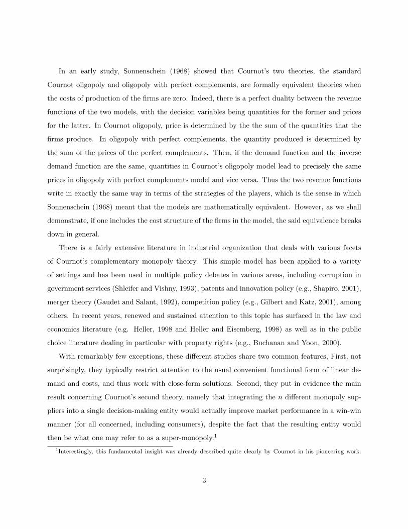
In an early study, Sonnenschein (1968) showed that Cournot’s two theories, the standard

Cournot oligopoly and oligopoly with perfect complements, are formally equivalent theories when

the costs of production of the firms are zero. Indeed, there is a perfect duality between the revenue

functions of the two models, with the decision variables being quantities for the former and prices

for the latter. In Cournot oligopoly, price is determined by the the sum of the quantities that the

firms produce. In oligopoly with perfect complements, the quantity produced is determined by

the sum of the prices of the perfect complements. Then, if the demand function and the inverse

demand function are the same, quantities in Cournot’s oligopoly model lead to precisely the same

prices in oligopoly with perfect complements model and vice versa. Thus the two revenue functions

write in exactly the same way in terms of the strategies of the players, which is the sense in which

Sonnenschein (1968) meant that the models are mathematically equivalent. However, as we shall

demonstrate, if one includes the cost structure of the firms in the model, the said equivalence breaks

down in general.

There is a fairly extensive literature in industrial organization that deals with various facets

of Cournot’s complementary monopoly theory. This simple model has been applied to a variety

of settings and has been used in multiple policy debates in various areas, including corruption in

government services (Shleifer and Vishny, 1993), patents and innovation policy (e.g., Shapiro, 2001),

merger theory (Gaudet and Salant, 1992), competition policy (e.g., Gilbert and Katz, 2001), among

others. In recent years, renewed and sustained attention to this topic has surfaced in the law and

economics literature (e.g. Heller, 1998 and Heller and Eisemberg, 1998) as well as in the public

choice literature dealing in particular with property rights (e.g., Buchanan and Yoon, 2000).

With remarkably few exceptions, these different studies share two common features, First, not

surprisingly, they typically restrict attention to the usual convenient functional form of linear de-

mand and costs, and thus work with close-form solutions. Second, they put in evidence the main

result concerning Cournot’s second theory, namely that integrating the n different monopoly sup-

pliers into a single decision-making entity would actually improve market performance in a win-win

manner (for all concerned, including consumers), despite the fact that the resulting entity would

then be what one may refer to as a super-monopoly.1

1Interestingly, this fundamental insight was already described quite clearly by Cournot in his pioneering work.

3

The main objectives of this paper may accordingly be described as follows. The first is to provide

a fairly extensive characterization of the general properties of oligopoly with perfect complements,

including basic theoretical preliminaries such as existence and uniqueness of equilibrium points.2 In

part, this amounts to a generalization of the many related results that have appeared in separate

contexts over a long period of time. In addition, since the present paper is based on the methodology

of supermodular games, this exercise also serves to provide a unifying framework for studies on this

model.3 The second objective is to qualify some conclusions about this model that have drawn close

parallels between Cournot’s two theories. The duality that Sonnenschein (1968) observed is actually

valid only in the absence of production costs. Similarly, based on a linear specification with nice

closed form solutions, Buchanan and Yoon (2000) also draw close analogies of both a qualitative and

a quantitative sort between the standard Cournot oligopoly (reflecting the commons in a way to be

made precise later) and Cournot’s complementary monopoly model (reflecting the anticommons).

Here again, it turns out that these rather striking analogies lack robustness in an essential way:

By incorporating linear costs of production into the two models, we show that the parallels largely

vanish.

In the overall presentation of the results of this paper, we discuss the relationship between

oligopoly with perfect complements and Cournot oligopoly. In particular, we point out the diver-

gences that are engendered by the incorporation of the cost structures into the two models. One

example of these differences is that while strategic complementarity of output levels in the stan-

dard Cournot oligopoly is not possible in the presence of non-trivial costs (Amir, 1996a), the prices

charged by the different monopolies in Cournot’s complementary monopoly model may well con-

stitute strategic complements to one another, albeit under general but restrictive assumptions on

demand and costs.

The rest of the paper is organized as follows. Section 2 provides a precise definition of Cournot’s

Cournot (1838) found that prices are lower and industry profits higher when a multi-product monopoly produces all

the goods instead of having n firms producing the goods.2Surprisingly, relative to the standard Cournot model where such studies have a long history (e.g., Novshek, 1985),

no general rigorous theoretic analysis of Cournot’s second model is available in the microeconomics literature (to the

best of our knowledge).3In particular, we invoke basic results and insights that have appeared in the application of these lattice-theoretic

tools in industrial organization theory (see Vives, 1990, 1995; Amir, 1996a; and Amir and Lambson, 2000).

4

second model and the basic existence proofs for both the asymmetric and the symmetric versions of

the model. Section 3 conducts a comparative statics analysis of market performance as the number

n of components of the system varies. Section 4 provides a generalization of the usual argument

in the literature about welfare and profit-enhancing integration. Finally, Section 5 deals with the

inclusion of production costs into the Buchanan and Yoon (2000) setting.

1.2 Some economic applications

This subsection discusses some of the applications of the model at hand in various areas of mi-

croeconomics. We provide only a short summary here, and refer the reader to the studies themselves

for further details and discussion.

One common application deals with patents (see Shapiro, 2001 and Lerner and Tirole, 2004).

This is clearly an application of oligopoly with perfect complements if we think of a firm or consumer

that wants to develop a new product but might infringe on a number of different patents owned by

different parties. Then, the developer has to pay for the usage of all of the patents involved. The

patents in this scenario are perfect complements and the consumer needs to buy a license for each

one of them.

In their study of corruption in government services, Shleifer and Vishny (1993) discuss the

common situation where a private developer needs different permits (e.g., from the fire, water and

police departments) to open a new business. This scenario fits into the present model if the officials

are assumed to be fully corrupt bribe maximizers.

Feinberg and Kamien (2001) analyze the hold-up problem that can arise in an oligopoly with

perfect complements when the acquisition of the multiple parts is sequential. For example, if the

government wishes to buy land from different owners in order to build a public project, one owner

can wait until the other owners have set prices for their land in order to get a higher benefit for her

part of land given that it is necessary for the project. Clearly, the small pieces of land owned by

different agents are perfect complements here.

Ellet (1966) uses the metaphor of two different owners of two sequential segments of a road where

there are no alternative routes or exits. Gardner, Gaston and Masson (2002) bring this analogy to

the real world and apply the oligopoly with perfect complements model to analyze how the Rhine

5

river was tolled in 12544.

A classical application of oligopoly with perfect complements is the anticommons problem.

This one arises when multiple agents have the right to exclude people from consuming the good

(anticommon good) that they own. This is modeled as each owner choosing the price for the

anticommon good that maximizes her profit, with the consumers having to pay each of the owners

their price in order to use the anticommon good. Buchanan and Yoon (2000) use as an example to

illustrate this problem a vacant lot that can be used as a parking lot that has a lower capacity than

its open demand. We will return to this example in the last section of the paper.

As shown by the previous examples, oligopoly with perfect complements is a model that has been

widely invoked in the literature. Nonetheless, there is a gap in terms of a general characterization

of its equilibria, which this paper hopes to fill.

2 The Model and some basic results

This section lays out the basic model of Cournot’s complementary monopoly and provides some

basic existence and uniqueness results. The general asymmetric case and the symmetric case are

considered separately. The reason for this is that, when insisting on minimal structural assumptions

on the model, the existence arguments are quite different across the two cases. In addition, beyond

the issues of existence and uniqueness, it is convenient to restrict attention to the symmetric case.

This is a key simplifying assumption of the analysis, which is further discussed later on.

Recall that an important auxiliary purpose of this paper is to address and partly correct a

widespread but imprecise perception in the literature that the two models that were put forward by

Cournot himself in 1938 are duals of one another in some fundamental ways. As the basic results

relating to this model are derived, we shall provide a brief comparison with the corresponding

results for standard Cournot oligopoly, and assess the similarities and the differences. To avoid

confusion between the two models, we shall for the most part refer to the present model as oligopoly

with perfect complements (instead of the historical and most commonly used name of Cournot’s

complementary monopoly). Therefore, we reserve the name of “standard Cournot oligopoly model”

4During the period 800-1800, 79 different locations served as toll stations along the Rhine river. The rights to

collect tolls were granted by the Emperor, who decided the number, location and amount charged at the toll stations.

6

for Cournot’s much more widely used model of quantity competition.

2.1 The Asymmetric Case

Consider an n-firm oligopoly with perfect complements, i.e., a market situation where each

of n producers sells one different good as a monopolist, and these goods are totally useless unless

purchased together in a fixed ratio to form a final product. W.l.o.g., we assume that this ratio is one-

to-one, since we can always appropriately re-normalize the quantities. In other words, consumers

wish to purchase a single system with demand function D(·), composed of n different components,

each of which is produced and sold by a separate firm acting as a monopoly supplier for that

component. This situation is modeled by letting each of the n firms set the price of its own

good/component and each consumer buy one unit of each of the n goods, paying the sum of all the

prices set by the firms.

This oligopoly with perfect complements is described by (n,K,D,Ci), where n is the number

of firms (or goods), K is the maximum price than can be charged for any of the goods in the

complementary market5, D : [0,∞) → [0,∞) is the demand function and Ci : [0,∞) → [0,∞) is

firm i’s cost function.

Denote the price that the firm under consideration charges by x and the sum of the prices of

the remaining (n − 1) firms by y. Let z = x + y represent the total price that a consumer has to

pay in order to obtain the system (of all the complementary goods).

Firm i chooses the price x ∈ [0,K] that maximizes its profit given by

πi(x, y) = xD(x+ y)− Ci[D(x+ y)]. (1)

Its reaction correspondence is

ri(y) = arg max{xD(x+ y)− Ci[D(x+ y)] : 0 ≤ x ≤ K}. (2)

Alternatively, we can think of the same firm as choosing z ∈ [y, y + K] given y, in this case, it

maximizes its profit given by

πi(z, y) = (z − y)D(z)− Ci[D(z)]. (3)

5The magnitude of K does not play any role in the proofs, so this is assumption is just for convenience.

7

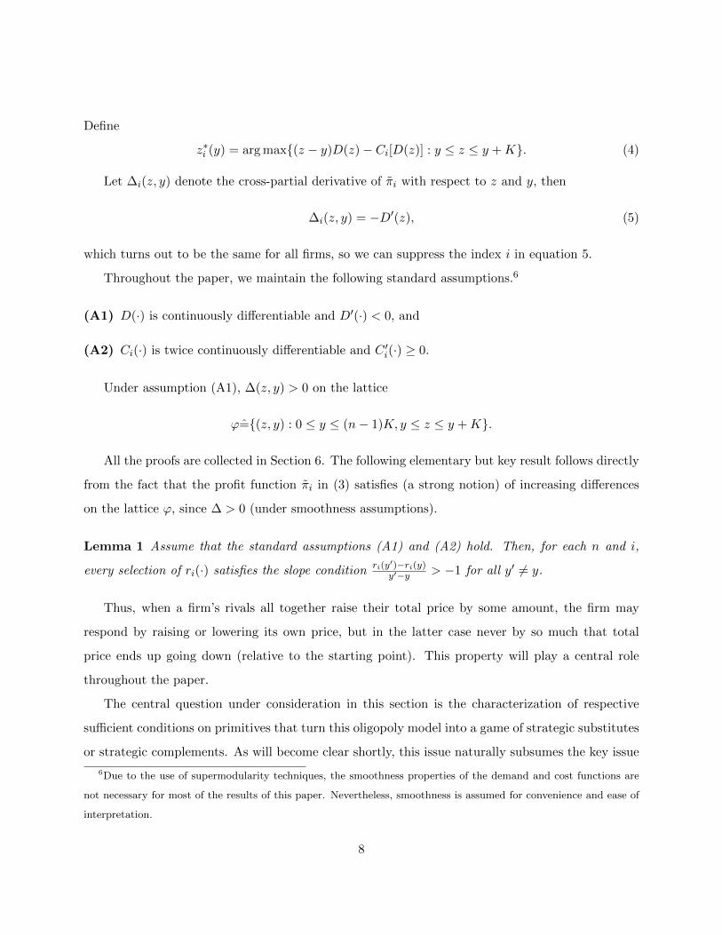
Define

z∗i (y) = arg max{(z − y)D(z)− Ci[D(z)] : y ≤ z ≤ y +K}. (4)

Let ∆i(z, y) denote the cross-partial derivative of πi with respect to z and y, then

∆i(z, y) = −D′(z), (5)

which turns out to be the same for all firms, so we can suppress the index i in equation 5.

Throughout the paper, we maintain the following standard assumptions.6

(A1) D(·) is continuously differentiable and D′(·) < 0, and

(A2) Ci(·) is twice continuously differentiable and C ′i(·) ≥ 0.

Under assumption (A1), ∆(z, y) > 0 on the lattice

ϕ={(z, y) : 0 ≤ y ≤ (n− 1)K, y ≤ z ≤ y +K}.

All the proofs are collected in Section 6. The following elementary but key result follows directly

from the fact that the profit function πi in (3) satisfies (a strong notion) of increasing differences

on the lattice ϕ, since ∆ > 0 (under smoothness assumptions).

Lemma 1 Assume that the standard assumptions (A1) and (A2) hold. Then, for each n and i,

every selection of ri(·) satisfies the slope condition ri(y′)−ri(y)y′−y > −1 for all y′ 6= y.

Thus, when a firm’s rivals all together raise their total price by some amount, the firm may

respond by raising or lowering its own price, but in the latter case never by so much that total

price ends up going down (relative to the starting point). This property will play a central role

throughout the paper.

The central question under consideration in this section is the characterization of respective

sufficient conditions on primitives that turn this oligopoly model into a game of strategic substitutes

or strategic complements. As will become clear shortly, this issue naturally subsumes the key issue

6Due to the use of supermodularity techniques, the smoothness properties of the demand and cost functions are

not necessary for most of the results of this paper. Nevertheless, smoothness is assumed for convenience and ease of

interpretation.

8

of existence of a pure-strategy Nash equilibrium (henceforth, PSNE) for this model. This is also

true in case the game is submodular since it clearly has the aggregation property (defined by the

fact that each payoff depends only on own action and on the sum of all other players’ actions).7

As the model at hand may be viewed as a special case of Bertrand competition with differentiated

products, one would expect the prototypical case to satisfy the strategic substitutes property since

the goods are complements in demand.8 The first result indicates that this expectation is essentially

correct in that it is fulfilled under quite a broad scope in terms of the restrictions needed on demand

and costs, as captured by the following assumptions on demand and costs.

Theorem 2 Assume that the standard assumptions (A1) and (A2) hold. Then, for each n ∈ N , if

D(·) is log-concave and Ci(·) is convex for all i, the oligopoly with perfect complements is a game

of strategic substitutes and there exists a unique PSNE.

The conditions of Theorem 2 are general enough as to capture most reasonable specifications

of Cournot’s complementary monopoly in applied settings, including the widely used case of linear

demand and costs (see below for such an example). It follows that one can consider this case to

represent the prototypical situation for this model.

Despite the fact that the game at hand is a special case of Bertrand competition with comple-

mentary products, it turns out that the scope for strategic complementarity of this game is clearly

non-trivial, as evidenced by the following (non-degenerate) sufficient conditions.

Theorem 3 Assume that the standard assumptions (A1) and (A2) hold. Then, for each n ∈ N , if

D(·) is log-convex and Ci(·) is concave for all i, the oligopoly with perfect complements is a game

of strategic complements and there exists a (not necessarily unique) PSNE.

7A pure-strategy Nash equilibrium for this model might be referred to in a number of different ways, either as a

Cournot equilibrium since the concept goes all the way back to the early book by Cournot (1838) or as a Bertrand

equilibrium since it deals with a form of price competition. Nonetheless, to avoid a potential for confusion, we shall

retain the neutral name of PSNE.8In Singh and Vives (1984), where the case of Bertrand competition with linear demand for differentiated products

is considered in some detail, the properties of strategic substitutes and strategic complements coincide exactly with the

properties of the goods being complements or substitutes in demand, respectively. However, for non-linear demands,

this is no longer true.

9

Log-convexity of demand is a rather restrictive condition. Of the commonly used examples, only

hyperbolic demand D(z) = 1/zα with α > 0 is log-convex. The limit case of a log-convex demand

function is the exponential demand, given by D(z) = e−z, z ≥ 0, which is strictly convex, log-linear,

thus (weakly) log-concave and log-convex.

Observing that the assumptions in the previous results are all in their weak form (as opposed

to their strict form), it follows as a direct corollary of the two Theorems that if demand is expo-

nential (i.e., D(z) = e−z, z ≥ 0) and the cost function is linear, then the resulting game must

be of both strategic substitutes and of strategic complements. In other words, the reaction curves

of all players must be constant functions. We report this formal Corollary in the form of an example.

Example 1. Consider an oligopoly with perfect complements with n firms/goods and a demand

function D(z) = e−z, z ≥ 0. Suppose that firm i faces a linear cost function Ci(q) = ciq ≥ 0 for

producing any output q ≥ 0. It is easy to derive the reaction curve of firm i (when rivals’ total price

is y ≥ 0) as

ri(y) = ci + 1 for any y ≥ 0.

In other words, each firm has a dominant strategy to price with a mark up of 1 (independent of

the actions of the firm’s rivals), thus leading to a unique PSNE price vector (c1 + 1, c2 + 1, ..., cn +

1). Consumers pay the total price of n +∑n

i=1 ci and each firm has equilibrium profit equal to

e−(n+∑n

i=1 ci). As mentioned, this example serves as an illustration of Theorems 2-3 as well as

Lemma 1.

With the general conditions for the existence of PSNE in hand, this ends our consideration

of the general case. Henceforth, we shall consider the symmetric case (with identical firms). In

particular, this will allow us to conduct comparative statics on the effects of exogenously changing

the number of firms based on lattice programming methods, with the number of firms being the

relevant parameter.

Comparing these existence results to those for standard Cournot oligopoly, many similarities

exist, but also one major difference. The latter model can enjoy strategic complementarities in a

global sense only in the abscence of (non-trivial) costs of production. In other words, while a similar

duality as the one reflected in the above results holds for the revenue function of Cournot firms, it

10

does not quite extend to the entire profit function. One consequence of this is that, when facing

an exponential inverse demand, Cournot firms have dominant strategies if and only if there are no

variable costs in production. For more details on these points, see Amir (1996a).

2.2 The Symmetric Case

Since each firm faces one and the same demand function for its (firm-specific) good or component,

to make all firms identical entails only the standard requirement for a symmetric oligopoly that the

firms have the same cost function for the production of their respective goods, denoted then by

C : [0,∞) → [0,∞).9 However, since these goods are not homogeneous in any way, the meaning

of identical cost functions is quite different from the standard one (say for Cournot oligopoly).

It typically does not entail access to the same technology, but rather that the different goods or

components cost the same to produce for the same number of units (given the postulated one-to-one

composition ratio).

The next Theorem establishes that the standard assumptions alone are sufficient to guarantee

the existence of at least one symmetric PSNE for the symmetric oligopoly with perfect complements,

and no asymmetric PSNEs.

Theorem 4 Assume that the standard assumptions (A1) and (A2) hold. Then, for each n ∈ N ,

the oligopoly with perfect complements has at least one symmetric equilibrium and no asymmetric

equilibria.

When all firms are identical, the property captured in Lemma 1, that a firm’s reaction curve

has all of its slopes bounded below by −1, is alone sufficient to yield existence of a (necessarily

symmetric) PSNE. This has no counterpart in the asymmetric version of the model.

Recall that a similar property holds in symmetric Cournot oligopoly in terms of output ad-

justment following a change in rivals’ total output, but not universally so. Indeed, in Amir and

Lambson (2000), the corresponding property holds only when production enjoys either decreasing

returns to scale or a limited form of scale economies.

9For ease of notation, whenever we refer to any of the variables or equations defining this model for now on, we

will drop the (firm) index i.

11

3 On the effects of varying the number of components

A proper study of this oligopoly model requires a good understanding of the effects that added

or reduced competition would have on equilibrium prices, per-firm output and profit. Although

we are asking how changes in the number of firms n affect these equilibrium variables, as in Amir

and Lambson (2000), the meaning of the question is somewhat different here. Instead of simple

entry or exit by one firm, the issue here is a comparison between the two situations where the exact

same final product that consumers want can be produced with either n or (n + 1) components,

with each firm’s cost function for a component being the same in both cases. Depending on the

precise context, the actual economic interpretation of this exercise may in fact reflect quite different

scenarios. For instance, in the context of a group of patents, it could be that one of the component

patents expires (thus implying a move from n to n − 1 patents) or that a new patent is added to

the group (a move from n to n+ 1 patents).10

While this specific question (involving intermediate values of n) has not really been addressed in

the literature on Cournot’s complementary monopoly, the comparison between monopoly and the

n-firm oligopoly is frequently assessed in specific formulations of this model (we shall have more on

this below). The answers provided here correspond to what one would expect, on the basis of the

specific formulations analyzed so far, in particular one with linear demand and costs.

As uniqueness of PSNE need not prevail for this model, we denote the equilibrium set for each

variable by its corresponding capital letter indexed by n. So with n firms, the equilibrium sets are

Xn for per-firm price, Yn for the firm’s (n − 1) rivals’ cumulative price, Zn for total price, Qn for

per-firm output, and Πn for per-firm output.

We say that an equilibrium set for a specific variable in the model is increasing or decreasing in

n, when the maximal and minimal points of the set are increasing or decreasing in n, respectively.11

10In the corrupt officials story of Shleifer and Vishny (1993), this might correspond to the government requiring

one extra permit (from a new official, say for hygiene) in addition to the existing list of permits. In tolling the

Rhine river, it could be that (for a variety of reasons) one of the owning entities decides to offer passage through its

own segment toll-free (this then corresponds to a decrease of n by one). Finally, it may be that a policy maker can

choose between two technology standards, one involving n components and the other (n + 1) components (with each

component produced by a monopolist with the same cost function).11This is a well-known feature of comparative statics conclusions based on supermodularity methods (see e.g.,

12

These are represented by an upper and a lower bar on the relevant variable, respectively.

Theorem 5 Under standard assumptions (A1) and (A2), for each n ∈ N,

(a) The equilibrium total price Zn is increasing in n; hence equilibrium per-firm output Qn is

decreasing in n.

(b) The equilibrium per-firm profit Πn is decreasing in n.

In oligopoly with perfect complements, the addition of one component to the system (or final

product) that perfectly complements the existing ones always increases the equilibrium total price.

This is very intuitive since now, there is an additional good that the consumer has to buy in order

to enjoy all of them. Also not surprisingly, the equilibrium profits of each of the existing firms

decreases (though the new monopolist increases from no profit to the same profit as all the others).

The results in Theorem 5 have been pointed out before in many particular economic applications,

often using particular functional forms. For instance, using the ubiquitous linear demand and

zero costs (see Section 5 below), Gardner, Gaston and Masson (2002) show that if the number of

segments in road tolling increases, the total price of the tolls goes up while the use of the road and

the individual profits of the tolls fall. Moreover, they find that the aggregate profits of the tolls also

fall. (The latter result is proved in full generality later on in this paper by Theorem 7.)

Shleifer and Vishny (1993) assert that when there is completely free entry of corrupt officials ask-

ing for a bribe to provide a service or good produced by the government, the total bribe approaches

infinity, driving the provision of the good and the bribe revenues towards zero.

We now investigate the direction of change of the equilibrium per-firm price Xn. As expected,

it can take either direction of change depending on the slope of the reaction curve with respect to

rivals’ cumulative price. Theorem 6 gives sufficient conditions for these directions of change. Notice

that, as can be seen from the proofs, it is an immediate consequence of Theorems 2-4 and Lemma

10 from the Appendix, which states that the equilibrium cumulative price of the rest of the (n− 1)

firms set is increasing in n.

Theorem 6 Assume that the standard assumptions (A1) and (A2) hold. Then, for each n ∈ N,

(a) If D(·) is log-convex and C(·) is concave, the equilibrium per-firm price Xn is increasing in n.

Milgrom and Roberts, 1990, 1994, and Echenique, 2002).

13

(b) If D(·) is log-concave and C(·) is convex, the (unique) equilibrium per-firm price xn is decreasing

in n.

As reported earlier, the prototypical case for oligopoly with perfect complements is characterized

by strategic substitutes, so that per-firm price will have a more pronounced tendency in general to

decrease with the number of components.

Now we turn to study what happens to the equilibrium consumer surplus, total profit and social

welfare sets when there is an exogenous change in the number of components. By Theorem 5 part

(a), the equilibrium total price increases with the number of firms and the equilibrium quantity

goes down. Thus, the equilibrium consumer surplus set decreases with more firms in the market.

Recall that by Theorem 5 part (b), the equilibrium individual profit decreases with the number

of products or firms. The following result tells us the stronger result that the equilibrium total

profit goes down as well. Combining these results, we conclude that equilibrium social welfare is

decreasing in n.

Theorem 7 Assume that the standard assumptions (A1) and (A2) hold, then, for each n ∈ N,

(a) Equilibrium consumer surplus CSn is decreasing in n.

(b) Equilibrium total profit nΠn is decreasing in n.

(c) Equilibrium social welfare Wn is decreasing in n.

In the literature on intellectual property rights, many experts have raised the concern that

innovation will have a tendency to be stifled in many high-tech industrial sectors by the increasing

number of patents. For biomedical research, see Heller and Eisemberg (1998) for more on this. In

fact, various calls for a major overhaul of the patenting system are being made both in the U.S.

and in Europe.

In some real world examples that fit the setting of oligopoly with perfect complements, the effects

captured in this section can lead to dramatically negative consequences for commerce. Shleifer and

Vishny (1993) report that, in Zaire, widespread corruption increases the costs of transportation

by land so much (due to the large amount of bribes that have to be paid along the way) that it

is cheaper to bring the same goods from Europe by ship. In a different but related matter, the

excessive number of tolls along the Seine in France around 1400 made shipping costs often more

14

expensive than the goods being transported themselves. In contrast, England was toll free, which

is often advanced as a key reason it became the center of commerce (Heilbroner, 1962).

Finally, we extend this analysis to the equilibrium price-cost margin, mn, defined by mn ,

xn −C ′[D(zn)]. In the empirical literature on market power, this is most often taken as a measure

of the level of competition in an industry.

For the model at hand, it turns out that it may increase or decrease with the number of firms

depending on whether the demand function is log-convex or log-concave.

Theorem 8 Suppose that the standard assumptions (A1) and (A2) hold. Then, for any n ∈ N ,

the equilibrium price-cost margin Mn is decreasing in n if D(·) is log-concave but increasing in n if

D(·) is log-convex.

From a comparison between the results in this Section and those in Amir and Lambson (2000),

it is clear that Cournot oligopoly and oligopoly with perfect complements are not mathematically

equivalent theories when the firms are symmetric and the production is costly.

Section 5 provides an explicit illustration of this fact.

4 Multi-product monopoly as the integrated solution

In the literature, the main focus is on the comparison between n-firm oligopoly with perfect

complements and the corresponding integrated solution wherein one multi-product monopolist offers

the entire system (of the same n components) at one overall price. Using the same notation as before,

the objective function of this n-product monopolist, who faces an n-fold cost of producing the same

amount of each component, is

Π(x) = xD(x)− nC[D(x)] (6)

It is important to observe that the concept of n-product monopolist is different from special case

n = 1 in the situation considered in the previous section, i.e., where the entire system amounts to

a single component. In other words, the n-product monopolist of this section is not obtained when

n = 1 is substituted in the model of the previous section (indeed, the objective of the latter would

then be maxx{xD(x)− C[D(x)]} instead of (6).

15

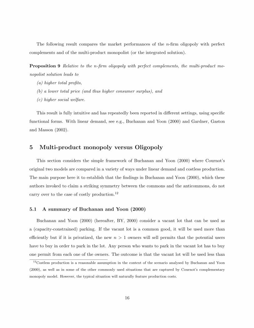
The following result compares the market performances of the n-firm oligopoly with perfect

complements and of the multi-product monopolist (or the integrated solution).

Proposition 9 Relative to the n-firm oligopoly with perfect complements, the multi-product mo-

nopolist solution leads to

(a) higher total profits,

(b) a lower total price (and thus higher consumer surplus), and

(c) higher social welfare.

This result is fully intuitive and has repeatedly been reported in different settings, using specific

functional forms. With linear demand, see e.g., Buchanan and Yoon (2000) and Gardner, Gaston

and Masson (2002).

5 Multi-product monopoly versus Oligopoly

This section considers the simple framework of Buchanan and Yoon (2000) where Cournot’s

original two models are compared in a variety of ways under linear demand and costless production.

The main purpose here it to establish that the findings in Buchanan and Yoon (2000), which these

authors invoked to claim a striking symmetry between the commons and the anticommons, do not

carry over to the case of costly production.12

5.1 A summary of Buchanan and Yoon (2000)

Buchanan and Yoon (2000) (hereafter, BY, 2000) consider a vacant lot that can be used as

a (capacity-constrained) parking. If the vacant lot is a common good, it will be used more than

efficiently but if it is privatized, the new n > 1 owners will sell permits that the potential users

have to buy in order to park in the lot. Any person who wants to park in the vacant lot has to buy

one permit from each one of the owners. The outcome is that the vacant lot will be used less than

12Costless production is a reasonable assumption in the context of the scenario analysed by Buchanan and Yoon

(2000), as well as in some of the other commonly used situations that are captured by Cournot’s complementary

monopoly model. However, the typical situation will naturally feature production costs.

16

efficiently. The first case illustrates the commons problem and the second one, the anticommons

one.

The commons problem can be seen as a Cournot oligopoly with n > 1 firms because the owners

of the common good decide how much of it to use in order to maximize their profits. Given that

the owners cannot exclude others from the usage of the common good, they maximize their profits

given the choice of usage of the other owners. The efficient level of usage of the good is equal to

the output that a monopolist would choose in this setting; thus, in this case, the relevant concept

of monopoly is given by the standard single-product monopolist.

On the other hand, the anticommons problem fits the setting of an oligopoly with perfect

complements with n > 1 firms. Firms are equivalent to “excluders” that choose the price of their

permits sold to the potential users in order for them to use the anticommon good. In this case,

the relevant concept of monopoly that provides the efficient level of permits (and thus, usage) is a

multi-product monopolist that sells all the permits as a bundle (with perfect complements).

BY(2000) solve the equilibrium for the four cases of interest under a linear demand and zero

costs. With inverse demand P (q) = a − bq, a single-product monopoly solves maxq q(a − bq) and

each firm in Cournot oligopoly solves maxq q(a− b(q + q′)) where y′ is rivals’ total output.

With direct demand D(z) = a−zb , the multi-product monopolist solves maxx x(a−xb ) and a firm

in the oligopoly with perfect complements solves maxx x(a−(x+y)b ) (with y defined as before).

The first three columns of Table 1 summarize the results in BY(2000).

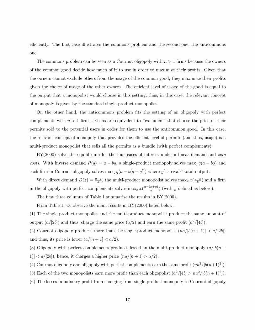
From Table 1, we observe the main results in BY(2000) listed below.

(1) The single product monopolist and the multi-product monopolist produce the same amount of

output (a/[2b]) and thus, charge the same price (a/2) and earn the same profit (a2/[4b]).

(2) Cournot oligopoly produces more than the single-product monopolist (na/[b(n + 1)] > a/[2b])

and thus, its price is lower (a/[n+ 1] < a/2).

(3) Oligopoly with perfect complements produces less than the multi-product monopoly (a/[b(n+

1)] < a/[2b]), hence, it charges a higher price (na/[n+ 1] > a/2).

(4) Cournot oligopoly and oligopoly with perfect complements earn the same profit (na2/[b(n+1)2]).

(5) Each of the two monopolists earn more profit than each oligopolist (a2/[4b] > na2/[b(n+ 1)2]).

(6) The losses in industry profit from changing from single-product monopoly to Cournot oligopoly

17

BY(2000) Present paper

(c=0) (c>0)

n > 1 Q∗BY P ∗BY Π∗BY Q∗ P ∗ Π∗

Single-product

monopoly

a2b

a2

a2

4ba−c2b

a+c2

(a−c)24b

Cournot oligopoly, n

firms

nab(n+1)

an+1

na2

b(n+1)2n(a−c)b(n+1)

a+ncn+1

n(a−c)2b(n+1)2

Loss in profit from 1 to

n firms

a2(n−1)24b(n+1)2

(a−c)2(n−1)24b(n+1)2

Multi-product

monopoly, n goods

a2b

a2

a2

4ba−nc2b

a+nc2

(a−nc)24b

Oligopoly with perfect

complements, n firms

ab(n+1)

nan+1

na2

b(n+1)2a−ncb(n+1)

n(a+c)n+1

n(a−nc)2b(n+1)2

Loss in profit from 1 to

n firms

a2(n−1)24b(n+1)2

(a−nc)2(n−1)24b(n+1)2

Table 1: equilibrium total output (Q∗), equilibrium total price (P ∗) and equilibrium industry profit

(Π∗) for different settings. The subindex BY stands for the results in BY(2000).

18

and from multi-product monopoly to oligopoly with perfect complements are the same (a2(n −

1)2/[4b(n+ 1)2]).

Based on the similarity shown in items (1) and (4)-(6), BY(2000) conclude that Cournot

oligopoly and oligopoly with perfect complements lead to symmetric tragedies. In particular, these

tragedies are reflected in the profit losses of changing from one to n firms having the same magnitude

in both models.

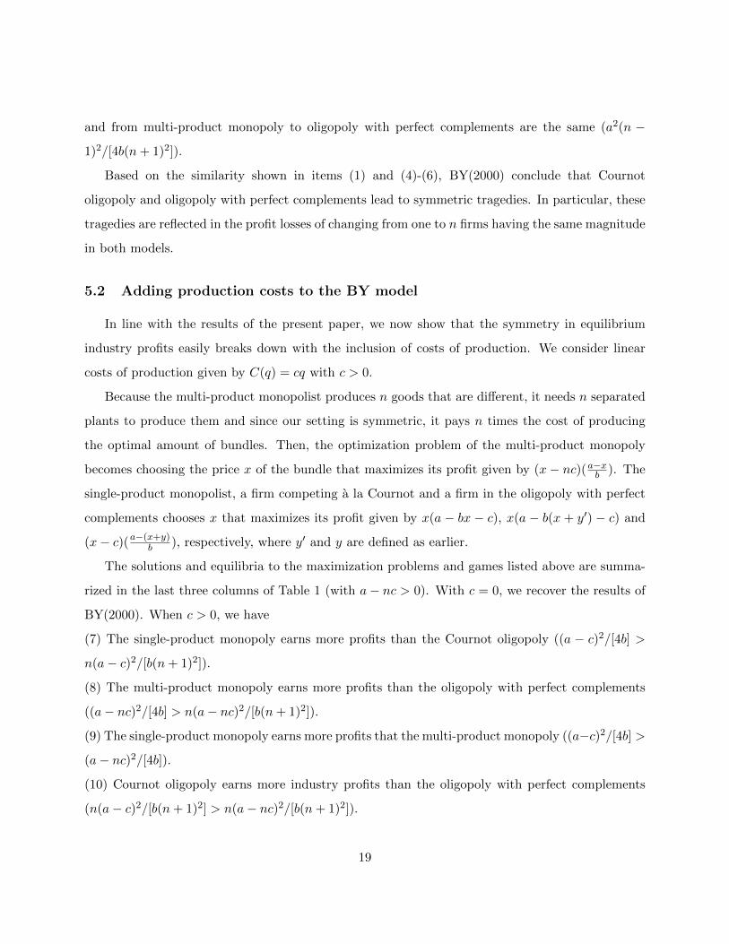
5.2 Adding production costs to the BY model

In line with the results of the present paper, we now show that the symmetry in equilibrium

industry profits easily breaks down with the inclusion of costs of production. We consider linear

costs of production given by C(q) = cq with c > 0.

Because the multi-product monopolist produces n goods that are different, it needs n separated

plants to produce them and since our setting is symmetric, it pays n times the cost of producing

the optimal amount of bundles. Then, the optimization problem of the multi-product monopoly

becomes choosing the price x of the bundle that maximizes its profit given by (x− nc)(a−xb ). The

single-product monopolist, a firm competing a la Cournot and a firm in the oligopoly with perfect

complements chooses x that maximizes its profit given by x(a − bx − c), x(a − b(x + y′) − c) and

(x− c)(a−(x+y)b ), respectively, where y′ and y are defined as earlier.

The solutions and equilibria to the maximization problems and games listed above are summa-

rized in the last three columns of Table 1 (with a− nc > 0). With c = 0, we recover the results of

BY(2000). When c > 0, we have

(7) The single-product monopoly earns more profits than the Cournot oligopoly ((a − c)2/[4b] >

n(a− c)2/[b(n+ 1)2]).

(8) The multi-product monopoly earns more profits than the oligopoly with perfect complements

((a− nc)2/[4b] > n(a− nc)2/[b(n+ 1)2]).

(9) The single-product monopoly earns more profits that the multi-product monopoly ((a−c)2/[4b] >

(a− nc)2/[4b]).

(10) Cournot oligopoly earns more industry profits than the oligopoly with perfect complements

(n(a− c)2/[b(n+ 1)2] > n(a− nc)2/[b(n+ 1)2]).

19

(11) The loss in industry profit of changing from single-product monopoly to Cournot oligopoly is

bigger than the loss in industry profit of having an oligopoly with perfect complements instead of

a multi-product monopoly ((a− c)2(n− 1)2/[4b(n+ 1)2] > (a− nc)2(n− 1)2/[4b(n+ 1)2]).

Thus, we have illustrated that the effects on industry profits of adding (n − 1) firms to the

single-product monopolist are in general, different from the effects on industry profits when we have

an oligopoly with perfect complements instead of a multi-product monopoly.

The idea that the tragedies of the commons and anticommons are not symmetric is discussed by

Vanneste, Van Hiel, Parisi and Depoorter (2006). Using two experiments, a lab experiment versus

a scenario experiment, they conclude that the behaviors of the players facing the same versions

of a commons dilemma and an anticommons dilemma are different. In particular, they find that

the players act more aggressively (with higher decision variables) when they face the anticommons

dilemma. Although this might be explained through the specification of the demand function, this

paper brings up the concern that the commons and anticommons problems are not symmetric in

general.

6 Proofs

We begin by defining a key mapping for every n ∈ N , which can be thought of as a normalized

cumulative best-response correspondence. This mapping is analogous to the one used by Amir and

Lambson (2000) and is useful in dealing with symmetric equilibria in the present context too.

Bn : [0, (n− 1)K] −→ 2[0,(n−1)K]

where

Bn(y) =n− 1

n(x′ + y). (7)

Here, x′ represents the firm’s best-response, i.e., the price that maximizes its profit in (1) given

the cumulative price y for the remaining (n− 1) firms. If x′ ∈ [0,K] and y ∈ [0, (n− 1)K], then the

(set-valued) range of Bn is as given. Also, a fixed point of Bn, y, clearly yields a symmetric PSNE

where x′ = y/(n− 1), i.e., each of the responding firms will set the same price as the other (n− 1)

firms.

20

Proof of Lemma 1.

Under (A1), the cross partial derivative of the maximand in (3), ∆(z, y), is strictly positive on the

lattice

ϕ = {(z, y) : 0 ≤ y ≤ (n− 1)K, y ≤ z ≤ y +K}.

The feasible set [y, y + K] is ascending in y. Then, by a strengthening of the basic monotonicity

theorem of Topkis (1978) due to Amir (1996c) and Edlin and Shannon (1998), every selection of z∗i

is strictly increasing in y as long as it is interior.

Since z∗i (y) = ri(y) + y, it follows directly that ri(·) has the given slope property.�

Proof of Theorem 2.

By a dual argument to Theorem 3 (proved below), the profit πi(x, y) exhibits the dual single-crossing

property under the hypotheses of the Theorem. Since the game at hand is an aggregative game of

strategic substitutes, by Tarski (1955) and Novshek (1985), an equilibrium exists.

To show that there is a unique PSNE, use Lemma 1 and the first part of this proof to conclude

that all the slopes (of all the selections) of ri(·) lie in (−1, 0]. Then, by a well known (contraction-

like) argument, the equilibrium is unique (see e.g., Amir, 1996b). �

Proof of Theorem 3. Milgrom and Shannon (1994) prove, for a Bertrand duopoly with differ-

entiated and complementary products, that if each demand function Di(x, y) is log-supermodular

and the cost function is concave, then πi(x, y) satisfies the single-crossing property in (x, y). Since

log-supermodularity of Di(x, y) translates into the log-convexity of D(x+y) in our setting, the proof

of this Theorem follows as a special case of their result. Hence, the game is a game of strategic

complements and by Tarski’s fixed-point Theorem (Tarski, 1955), an equilibrium exists. �

Proof of Theorem 4.

By the proof of Lemma 1, every selection of z∗ is increasing in y. Recall that x′ denotes the firm’s

best-response to y, thus z∗(y) = x′ + y. This implies that for every n ∈ N , every selection of Bn

21

as defined by equation (7) is increasing in y. Then, by Tarski’s fixed-point Theorem, (any selection

of) Bn has a fixed-point that implies the existence of a symmetric equilibrium of the oligopoly with

perfect complements.

Next, we prove that no asymmetric equilibrium can exist. By the proof of Lemma 1, every

selection of z∗ is strictly increasing. This means that for each z′ ∈ z∗ corresponds at most one y

such that z′ = x′ + y (z′ is the best-response to y); then, for each total equilibrium price z′, each

firm must charge the same price x′ = z′ − y, with y = (n − 1)x′, i.e., no asymmetric equilibrium

exists. �

Before proceeding with the rest of the proofs, we need the following intermediate Lemmas.

Lemma 10 Assume that the standard assumptions (A1) and (A2) hold. Then, for every number

of firms n ∈ N , the equilibrium cumulative prices of (n− 1) firms set, Yn, is increasing in n.

Proof of Lemma 10.

By Topkis’s Theorem, the maximal and minimal selections of Bn, denoted by Bn and Bn respec-

tively, exist. Furthermore, the largest equilibrium cumulative price for (n − 1) firms, yn, is the

largest fixed-point of Bn. Bn(y) is increasing in n for every fixed y. Hence, by Theorem A.4 in

Amir and Lambson (2000), the largest fixed-point of Bn, yn, is also increasing in n. Using an

analogous argument with Bn shows that the the smallest equilibrium cumulative price for (n − 1)

firms, yn, is increasing in n. �

Lemma 11 Assume that the standard assumptions (A1) and (A2) hold. Then, for every number

of firms n ∈ N , πn = π(xn, (n− 1)xn) ≥ πn = π(xn, (n− 1)xn).

Proof of Lemma 11.

We prove that πn = π(xn, (n − 1)xn), a similar argument shows that πn = π(xn, (n − 1)xn). To

this aim, observe that π(z, y) is decreasing in y, then, πn = π(zn,(n−1)n zn) = π(xn, (n − 1)xn).

Now, we show that πn = π(xn, (n − 1)xn). Suppose not, then it exists xn ∈ Xn such that

π(xn, (n−1)xn) > π(xn, (n−1)xn), then, π(xn, (n−1)xn) = π(zn,(n−1)n zn) > π(xn, (n−1)xn) = πn,

22

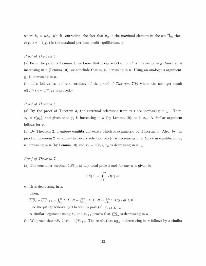
where zn = nxn, which contradicts the fact that πn is the maximal element in the set Πn, thus,

π(xn, (n− 1)xn) is the maximal per-firm profit equilibrium. �

Proof of Theorem 5.

(a) From the proof of Lemma 1, we know that every selection of z∗ is increasing in y. Since yn is

increasing in n (Lemma 10), we conclude that zn is increasing in n. Using an analogous argument,

zn is increasing in n.

(b) This follows as a direct corollary of the proof of Theorem 7(b) where the stronger result

nπn ≥ (n+ 1)πn+1 is proved.�

Proof of Theorem 6.

(a) By the proof of Theorem 3, the extremal selections from r(·) are increasing in y. Then,

xn = r(yn), and given that yn is increasing in n (by Lemma 10), so is xn. A similar argument

follows for xn.

(b) By Theorem 2, a unique equilibrium exists which is symmetric by Theorem 4. Also, by the

proof of Theorem 2 we know that every selection of r(·) is decreasing in y. Since in equilibrium yn

is increasing in n (by Lemma 10) and xn = r(yn), xn is decreasing in n. �

Proof of Theorem 7.

(a) The consumer surplus, CS(·), at any total price z and for any n is given by

CS(z) =

∫ ∞z

D(t) dt,

which is decreasing in z.

Then,

CSn − CSn+1 =∫∞znD(t) dt−

∫∞zn+1

D(t) dt =∫ zn+1zn

D(t) dt ≥ 0.

The inequality follows by Theorem 5 part (a), zn+1 ≥ zn.

A similar argument using zn and zn+1 proves that CSn is decreasing in n.

(b) We prove that nπn ≥ (n + 1)πn+1. The result that nπn is decreasing in n follows by a similar

23

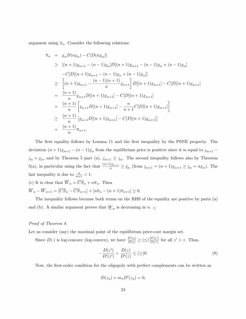
argument using xn. Consider the following relations:

πn = xnD(nxn)− C[D(nxn)]

≥ [(n+ 1)xn+1 − (n− 1)xn]D[(n+ 1)xn+1 − (n− 1)xn + (n− 1)xn]

−C[D[(n+ 1)xn+1 − (n− 1)xn + (n− 1)xn]]

≥[(n+ 1)xn+1 −

(n− 1)(n+ 1)

nxn+1

]D[(n+ 1)xn+1]− C[D[(n+ 1)xn+1]

=(n+ 1)

nxn+1D[(n+ 1)xn+1]− C[D[(n+ 1)xn+1]

=(n+ 1)

n

[xn+1D[(n+ 1)xn+1]−

n

n+ 1C[D[(n+ 1)xn+1]

]≥ (n+ 1)

n

[xn+1D[(n+ 1)xn+1]− C[D[(n+ 1)xn+1]

]=

(n+ 1)

nπn+1.

The first equality follows by Lemma 11 and the first inequality by the PSNE property. The

deviation (n+ 1)xn+1 − (n− 1)xn from the equilibrium price is positive since it is equal to zn+1 −

zn + xn, and by Theorem 5 part (a), zn+1 ≥ zn. The second inequality follows also by Theorem

5(a), in particular using the fact that(n+1)xn+1

n ≥ xn (from zn+1 = (n+ 1)xn+1 ≥ zn = nxn). The

last inequality is due to nn+1 < 1.

(c) It is clear that Wn = CSn + nπn. Then

Wn −Wn+1 = [CSn − CSn+1] + [nπn − (n+ 1)πn+1] ≥ 0.

The inequality follows because both terms on the RHS of the equality are positive by parts (a)

and (b). A similar argument proves that Wn is decreasing in n. �

Proof of Theorem 8.

Let us consider (say) the maximal point of the equilibrium price-cost margin set.

Since D(·) is log-concave (log-convex), we have D′(z)D(z) ≥ (≤)D

′(z′)D(z′) for all z′ > z. Thus,

−D(z′)

D′(z′)+D(z)

D′(z)≤ (≥)0. (8)

Now, the first-order condition for the oligopoly with perfect complements can be written as

D(zn) +mnD′(zn) = 0,

24

which implies that

mn = −D(zn)

D′(zn).

If D(·) is log-concave (log-convex), mn is decreasing (increasing) in zn, then, mn = − D(zn)D′(zn)

(mn = − D(zn)D′(zn)

).

Thus, mn+1 −mn = − D(zn+1)

D′(zn+1)+

D(zn)D′(zn)

(mn+1 −mn = − D(zn+1)

D′(zn+1)+ D(zn)

D′(zn)

), which is negative

(positive) if D(·) is log-concave (log-convex), by equation 8 and Theorem 5 part (a), zn+1 ≥ zn

(zn+1 ≥ zn). �

Proof of Proposition 9.

(a) This follows from a rather standard argument. Since the n-product monopolist can replicate

whatever price vector the oligopoly can use, it is obvious that the former can achieve a higher total

profit than the latter.

(b) The sum (across the n firms) of the first order conditions at a symmetric PSNE is (where z

stands for total price)

nD(z) + zD′(z)− nC ′[D(z)]D′(z) = 0. (9)

From equation (6), the first order condition for the n-product monopolist’s solution is (where z

stands for total price)

D(z) + zD′(z)− nC ′[D(z)]D′(z) = 0. (10)

Since for any n > 1, the LHS of (9) is an upward shift of the LHS of (10), the extremal solutions

(which are the extremal zeros of the LHS’s) of (9) are higher than those of (10).

Hence, price is lower for the n-product monopolist. It follows that consumer surplus is higher

with the n-product monopolist.

(c) This follows directly from (a) and (b).�

25

References

[1] Amir, R., 1996a, Cournot oligopoly and the theory of supermodular games, Games and Eco-

nomic Behavior, 15, 132-148.

[2] Amir, R., 1996b, Continuous stochastic games of capital accumulation with convex transitions,

Games and Economic Behavior, 15, 111-131

[3] Amir, R., 1996c, Sensitivity analysis in multisector optimal economic dynamics, Journal of

Mathematical Economics, 25, 123-141.

[4] Amir, R. and V. E. Lambson, 2000, On the effects of entry in Cournot markets, Review of

Economic Studies, 67, 235-254.

[5] Buchanan, J. M. and Yoon, Y. J., 2000, Symmetric tragedies: commons and anticommons,

The Journal of Law and Economics, 43, 1-13.

[6] Cournot, A., 1960 [1838], Researches into the Mathematical Principles of the Theory of Wealth,

Augustus M. Kelley.

[7] Echenique, F. (2002), Comparative statics by adaptive dynamics and the correspondence prin-

ciple, Econometrica 70, 833-844.

[8] Edlin, A. and C. Shannon (1998), Strict monotonicity in comparative statics, Journal of Eco-

nomic Theory 81, 201-219.

[9] Ellet, C., 1966 [1839], An Essay on the Laws of Trade in Reference to the Works of Internal

Improvement in the United States, Augustus M. Kelley.

[10] Feinberg, Y. and Kamien, M. I., 2001, Highway robbery: complementary monopoly and the

hold-up problem, International Journal of Industrial Organization, 19, 1603-1621.

[11] Gardner, R., Gaston, N. and Masson, R. T., 2002, Tolling the Rhine in 1254: complementary

monopoly revisited.

[12] Gaudet, G. and S. Salant, 1992, Mergers of producers of perfect complements competing in

price, Economics Letters, 39, 359-364.

26

[13] Gilbert, R.J. and Katz, L.M., 2001, An Economist’s Guide to U.S. v. Microsoft, Journal of

Economic Perspectives, 15: 25–44.

[14] Heilbroner, R. L., 1962, The Making of Economic Society, Prentice-Hall.

[15] Heller, M.A. and Eisemberg, R.S., 1998. Can patents deter innovation? The anticommons in

biomedical research, Science, 280: 698–701.

[16] Lerner, J. and Tirole, J., 2004, Efficient patent pools, American Economic Review, 94, 691-711.

[17] Milgrom, P. and Roberts, J., 1990, Rationalizability, learning, and equilibrium in games with

strategic complementarities, Econometrica, 58, 1255-1278.

[18] Milgrom, P. and Roberts, J., 1994, Comparing equilibria, American Economic Review, 84,

441-459.

[19] Milgrom, P. and Shannon, C., 1994, Monotone comparative statics, Econometrica, 62, 157-180.

[20] Novshek, W., 1985, On the existence of Cournot equilibrium, Review of Economic Studies, 52,

85-98.

[21] Shapiro, C., 1989, Theories of oligopoly behavior, Handbook of Industrial Organization, 1,

329-414.

[22] Shapiro, C., 2001, Navigating the patent thicket: cross licences, patent pools, and standard

setting, Innovation Policy and the Economy, Volume 1, MIT Press, 119-150.

[23] Shleifer, A. and Vishny, R. W., 1993, Corruption, The Quarterly Journal of Economics, 108,

599-617.

[24] Singh, N. and Vives, X., 1984, Price and quantity competition in a differentiated duopoly, Rand

Journal of Economics, 15, 546-554.

[25] Sonnenschein, H., 1968, The dual of duopoly is complementary monopoly: or, two of Cournot’s

theories are one, Journal of Political Economy, 76, 316-318.

27

[26] Tarski, A., 1955, A lattice-theoretical fixpoint theorem and its applications, Pacific Journal of

Mathematics, 5, 285-309.

[27] Topkis, D. M., 1978, Minimizing a submodular function on a lattice, Operations Research, 26,

305-321.

[28] Topkis, D. M., 1979, Equilibrium points in nonzero-sum n-person submodular games, SIAM,

Control and Optimization, 17, 773-787.

[29] Vanneste, S., Van Hiel, A., Parisi, F. and Depoorter, B., 2006, From “tragedy” to “disas-

ter”: welfare effects of commons and anticommons dilemmas, International Review of Law and

Economics, 26, 104-122.

[30] Vives, X. (1990), Nash equilibrium with strategic complementarities, Journal of Mathematical

Economics, 19, 305-321.

28