Embed Size (px)
Citation preview

On convex envelopes andunderestimators for bivariate
functions
Marco Locatelli
Dipartimento di Ingegneria Informatica, Universita di ParmaVia G.P. Usberti, 181/A, 43124 Parma, Italy
e-mail: [email protected]
Fabio Schoen
Dipartimento di Sistemi e Informatica, Universita di FirenzeVia di Santa Marta, 3, 50139 Firenze, Italy
e-mail: [email protected]
Abstract
In this paper we discuss convex underestimators for bivariate func-tions. We first present a method for deriving convex envelopes over thesimplest two-dimensional polytopes, i.e., triangles. Next, we proposea technique to compute the value at some point of the convex envelopeover a general two-dimensional polytope, together with a supportinghyperplane of the convex envelope at that point. Noting that the en-velopes might be of quite complicated form and their computation noteasy, we move later on to the discussion of a method, based on thesolution of a semidefinite program, to derive convex underestimators(not necessarily convex envelopes) of simple enough form for bivariatequadratic functions over general two-dimensional polytopes.
KEYWORDS: convex envelopes, convex underestimators, semidefinite pro-gramming, quadratic problems.
1 Introduction
Convex underestimators of a nonconvex function f over some region X arevery important in the development of branch-and-bound techniques for thesolution of global optimization problems. The best (largest) possible of suchunderestimators is called convex envelope of f over X. Unfortunately, thederivation of the convex envelope is not a simple task. For instance, in [6] itis proved that finding the convex envelope of a multilinear function (linear
1

combination of products of variables) over the unit hypercube is NP-hard, al-though envelopes can be computed for special cases (see, e.g., [7, 16, 17, 19]).In general, the difficulty is related to the nonlinear function f to be under-estimated and/or the region X over which we want to compute the envelope(see also a similar comment, e.g., in [9]). Usually, we are not able to findthe envelope of f over the region X we are interested at, but it is sometimespossible to find the envelope over a region M ⊇ X. Of course, the closer isM to X, the better is the approximation delivered by the envelope. Usualchoices for M are (hyper)rectangles. For the bilinear function xy convexand concave envelopes over rectangles have been derived in [14] and latervalidated in [2]. For the fractional term y/x in [24] the concave envelopeover a rectangle in the positive orthant has been derived, while in [20] theresult has been extended also to rectangles which do not lie in the positiveorthant. In [18] convex envelopes of the bilinear term over special polytopes,the D-polytopes, have been derived. D-polytopes are characterized by thefact that they do not contain edges with finite positive slope. In [4] the en-velopes of the fractional term over special bounded quadrilaterals over R
2
(parallelograms and trapezoids) have been derived. In [13] the convex en-velope of the bilinear term over triangles with a single edge having positiveslope is presented, while in [3] a representation of the convex envelope overgeneral triangles through doubly nonnegative matrices (i.e., matrices whichare both semidefinite and nonnegative) is given. Some literature about con-vex envelopes is dedicated to the detection of the cases with a polyhedralconvex envelope, i.e., cases where the convex envelope is the maximum of afinite number of affine functions. In [15, 23] edge-concave functions over apolytope P (i.e., functions which are concave on all segments in P parallelto an edge of P ) are discussed and it is proved that they have a polyhedralconvex envelope. Another relevant result about polyhedral convex envelopesis presented in [16] and will be discussed later. Other results about convexenvelopes can be found in the literature (e.g., in [12] the convex envelopefor monomials with odd degree is derived) but those discussed up to nowalready show that convex envelopes can be computed only for simple enoughfunctions f and regions M . Even when they are computable, they might beof quite complicated form. Then we consider the following question. If thecomputation of the convex envelope of a function f over some region M istoo hard and/or the functional form of the envelope is too complicated, whatcould we do? An obvious answer is to give up the requirement of finding theconvex envelope and being satisfied with a convex underestimator of f overM . Reasonable requirements for such underestimator are the following:
• should be simple enough to compute;
2

• should be close enough to the function f ;
• M should approximate as tightly as possible the region X at which weare interested;
• should be of simple enough form.
For instance, in [1] it is proposed to underestimate a general nonconvex termover a box by summing up to it a convex quadratic function (nonpositive overthe box), so that the positive eigenvalues of the quadratic term compensatethe negative ones of the nonconvex term, making the result of the sum aconvex underestimator.The paper is organized as follows. In Section 2 we will propose a way tocompute the convex envelope of some bivariate functions over quite simpledomains like triangles and show that for some triangles (with two or threeedges along which the function is convex) the functional form of the envelopeis not simple at all. In Section 3 we further show that the computation of thevalue at some point of the convex envelope over a general two-dimensionalpolytope, together with a supporting hyperplane of the convex envelope atthat point, requires the solution of a number of three-dimensional convex sub-problems which might increase exponentially with the number of edges alongwhich the function is convex. In Section 4 we propose convex undestima-tors for indefinite bivariate quadratic functions over general two-dimensionalpolytopes. These will be called Quadratic Convex Underestimators (QCUs).Their computation will involve the solution of a semidefinite program whosesize increases with the number of vertices of the polytopes.
2 Convex envelopes of bivariate functions over
triangles
In this section we propose a method to derive the convex envelope over tri-angles for bivariate functions satisfying some conditions. Let T be a trianglewith vertices V1, V2, V3. Let f(x, y) be a bivariate function. We assume thefollowing conditions are satisfied:
Condition 1 the Hessian of f is indefinite in the interior of the triangle;
Condition 2 the restriction of f along each edge of the triangle is eitherconcave or strictly convex;
Condition 3 if f is strictly convex over all the three edges, then there existtwo edges such that f is also strictly convex along each segment joiningtwo points belonging to such edges.
3

For instance, function f(x, y) = xy satisfies the above conditions for allpossible triangles T . In particular, in this case edges along which the functionis strictly convex are those lying along lines with positive slope and the twoedges satisfying Condition 3 are those forming an obtuse angle. The bivariatefunction f(x, y) = x log(1 + y) satisfies the above conditions, e.g., over thetriangle T with
V1 =
(
00
)
V2 =
(
10
)
V3 =
(
11
)
We recall that, according to Caratheodory’s theorem, given a polytope P ⊂R
n and a function f , the convex envelope of f at a point K ∈ P is definedas follows
CEf,P (K) = min
{
n+1∑
i=1
λif(Qi) : Qi ∈ P, i = 1, . . . , n + 1,
n+1∑
i=1
λi = 1,
n+1∑
i=1
λiQi = K, λi ≥ 0
}
.
A relevant subset of P is the so called generating set denoted by X(f) anddefined as the smallest subset of P such that
CEf,P (K) = min
{
n+1∑
i=1
λif(Qi) : Qi ∈ X(f), i = 1, . . . , n + 1,
n+1∑
i=1
λi = 1,n+1∑
i=1
λiQi = K, λi ≥ 0
}
, (1)
i.e., the convex envelope of f over P is equal to its convex envelope over X(f).
The simplest case to deal with is when the convex envelope over a trian-gle is polyhedral, i.e., X(f) is equal to the set of vertices of the triangle.A fundamental result, which we report here for sake of completeness, is thefollowing:
Theorem 2.1 (from Theorem 1.2 in [16]) : Let f(x) be a lower semi-continuous function on a compact polytope P and for every point x0 whichis not a vertex there exists a line ℓx such that f(x) is a concave functionin a neighborhood of x0 on a segment (ℓx
⋂
P ) and x0 ∈ ri[ℓx
⋂
P ]. ThenconvP f(x) is a polyhedral function [. . . ].
4

Therefore, under the given conditions, this theorem clearly defines the caseswhere the convex envelope over a triangle is polyhedral: this holds when fis concave over all the three edges of the triangle. But the theorem actuallytells us something more. Indeed, its proof can be employed to show that thegenerating set X(f) is made up by all the vertices of the triangle plus all theedges along which the function f is convex and not concave (see also [21]).Therefore, besides the simplest polyhedral case we need to deal with threemore cases, those where the number of edges along which f is convex andnot concave is equal respectively to 1, 2 or 3. The analysis of such cases isstrictly related to the one in [11] and [20]. Both papers deal with multivariatefunctions, but here we describe their contents only for bivariate functions.In [11] techniques to derive convex envelopes of 1-convex bivariate functionsover boxes are discussed. 1-convex functions are bivariate functions f(x, y)whose Hessian is always indefinite but which are convex with respect to oneof the two variables when the other one is fixed. In [20] the convex envelopeover boxes is derived for bivariate functions f(x, y) which are convex withrespect to x when y is fixed, and concave with respect to y when x is fixed.In particular, the results are applied to derive the convex envelope of thefractional function y/x over a box. The results of both papers are based onthe fact that for functions satisfying the given assumptions over boxes, itturns out that the minimum in (1) for a point K 6∈ X(f), and belonging tothe box, is attained with just two points Q1, Q2 belonging to X(f). Here weprove that, for the three cases mentioned above, the same holds for bivariatefunctions satisfying Conditions 1-3 over triangles. This is the result of thefollowing lemma.
Lemma 2.1 Given a triangle with vertices V1, V2, V3, let ℓ be the number ofedges along which the function is convex and not concave. Then the minimumin (1) for a point K 6∈ X(f) and belonging to the triangle is attained:
1. with Qi = Vi, i = 1, 2, 3, i.e. points Qi’s are the three vertices belongingto X(f) for ℓ = 0;
2. with just two points Q1, Q2 ∈ X(f), one being the vertex opposite to theconvex edge and the other lying along the convex edge itself for ℓ = 1;
3. with just two points Q1, Q2 ∈ X(f), one belonging to a convex edge andthe other lying along the other convex edge for ℓ = 2;
4. with just two points Q1, Q2 = X(f), one belonging to one of the twoedges satisfying Condition 3 and the other belonging to the third edge.
Proof.
5

1. immediately follows from Theorem 2.1.
2. the minimum in (1) is attained for (at most) three points lying inX(f). First of all we notice that the three points can not all lie alongthe convex edge, because no convex combination of three points alongthe edge can return a point outside the edge. Therefore, one of thepoints must be in the unique point in X(f) outside the convex edge,i.e., the vertex opposite to the convex edge, say V1. Next, let us assumethat the other two points, denoted by Q′ and Q′′, lie along the convexedge. Then, we must have that
K = λ1Q′+λ2Q
′′+λ3V1 and CEf,T (K) = λ1f(Q′)+λ2f(Q′′)+λ3f(V1),
with λ1, λ2, λ3 > 0. But if we consider the point
Q =λ1
λ1 + λ2Q′ +
λ2
λ1 + λ2Q′′,
it holds thatK = (λ1 + λ2)Q + λ3V1
and, in view of the convexity of f along the edge,
(λ1 + λ2)f(Q) ≤ λ1f(Q′) + λ2f(Q′′),
so that we can replace the two points Q′, Q′′ with the single one Qbelonging to the convex edge.
3. in case we have exactly three points, at least two of them must belongto the same edge. As in the proof of Point 2, convexity of f oversuch edge allows to substitute the two points along the edge with theirconvex combination, so that the conditions of the lemma are satisfied.
4. by the standard argument already employed for the proofs of Points 2and 3, we know that the three points, say Q′, Q′′, Q′′′, must all lie ondistinct edges. Now, let Q′ and Q′′ lie along the two edges satisfyingCondition 3. Then, function f is strictly convex along the line throughQ′ and Q′′, so that we could substitute these two points with theirconvex combination, contradicting the optimality of the three pointsQ′, Q′′, Q′′′. Therefore, we can restrict our attention to just two points,one of which should lie along one of the two edges satisfying Condition3 and the other belonging to the third edge.
6

2
The above remark can be employed to derive the convex envelope of functionf over triangles. It will turn out that when ℓ = 0, 1, for a given point withinthe triangle, we will be able to immediately identify the points giving theminimum value in (1), while for the cases ℓ = 2, 3 the identification of thepoints will require the solution of a one-dimensional problem.
Theorem 2.2 For a given point K in the triangle, it holds that the convexenvelope of f at K is:
ℓ = 0 the value at K of the unique affine function whose value at the threevertices are equal to the corresponding values of f at the vertices;
ℓ = 1 the valueλ∗f(V1) + (1 − λ∗)f(H),
where H is the point at the intersection of the convex edge and the linethrough V1 and K and λ∗ ∈ [0, 1] is the unique value such that
K = λ∗V1 + (1 − λ∗)H.
ℓ = 2, 3 the solution of a properly defined minimization problem of a one-dimensional function.
Proof.
ℓ = 0 this case is well known and does not need to be proved.
ℓ = 1 The result is an immediate consequence of Point 2 in Lemma 2.1,stating that the minimum of (1) is attained at points V1 and H , whereH is the unique point along the convex edge lying along the line throughV1 and K.
ℓ = 2 let ¯V1V3 and ¯V2V3 be the two edges along which function f is convex.There exist unique values λ1, λ2, λ3 ≥ 0,
∑3i=1 λi = 1, such that
K = λ1V1 + λ2V2 + λ3V3.
In view of Point 3 in the Lemma 2.1, it holds that the optimal value of(1) is attained at two points
Q = µV1 + (1 − µ)V3 µ ∈ [0, 1]
7

Q′ = αV2 + (1 − α)V3 α ∈ [0, 1]
such that K ∈ QQ′, i.e.
K = ξQ + (1 − ξ)Q′ ξ ∈ [0, 1].
By substitution we get
K = ξ(µV1 + (1 − µ)V3) + (1 − ξ)(αV2 + (1 − α)V3) =
= µξV1 + (1 − ξ)αV2 + [(1 − µ)ξ + (1 − ξ)(1 − α)]V3
By the uniqueness of the λi values, it must hold that
ξµ = λ1
α(1 − ξ) = λ2
and, consequently
ξ = λ1/µ
α =µλ2
µ − λ1
Note that
ξ ∈ [0, 1] ⇒ µ ≥ λ1, α ∈ [0, 1] ⇒ µ ≥ λ1/(1 − λ2).
Then, if we want to detect the value of the convex envelope at K, weneed to solve the following one-dimensional minimization problem
minµ∈[λ1/(1−λ2),1]
λ1
µf(Q) +
(
1 − λ1
µ
)
f(Q′),
or, equivalently
minµ∈[λ1/(1−λ2),1]λ1
µf (µV1 + (1 − µ)V3) +
+
(
1 − λ1
µ
)
f
(
µλ2
µ − λ1V2 +
(
1 − µλ2
µ − λ1
)
V3
)
.
ℓ = 3 Let ¯V1V2 and ¯V2V3 be the two edges satisfying Condition 3. As before,there exist unique values λ1, λ2, λ3 ≥ 0,
∑3i=1 λi = 1, such that
K = λ1V1 + λ2V2 + λ3V3.
8

In view of Point 4 in Lemma 2.1, it holds that the optimal value of (1)is attained at two points, one belonging to the edge ¯V1V3 different fromthe two satisfying Condition 3
Q = µV1 + (1 − µ)V3 µ ∈ [0, 1],
the other one either belonging to the edge ¯V2V3:
Q′ = αV2 + (1 − α)V3 α ∈ [0, 1]
or to the edge ¯V1V2:
Q′′ = βV1 + (1 − β)V2 β ∈ [0, 1]
Therefore, either K ∈ QQ′, i.e.
K = ξQ + (1 − ξ)Q′ ξ ∈ [0, 1]
or K ∈ ¯QQ′′, i.e.
K = ηQ + (1 − η)Q′′ η ∈ [0, 1].
In particular, by taking the intersection of ¯V1V3 with the line throughV2 and K, it holds that
K ∈ QQ′ ⇒ µ ∈ [λ1/(1 − λ2), 1]
whileK ∈ ¯QQ′′ ⇒ µ ∈ [0, λ1/(1 − λ2)]
The case K ∈ QQ′ leads to a result completely analogous to what al-ready seen in Point 3 and leads to the following one-dimensional func-tion
g1(µ) =λ1
µf (µV1 + (1 − µ)V3)+
(
1 − λ1
µ
)
f
(
µλ2
µ − λ1V2 +
(
1 − µλ2
µ − λ1
)
V3
)
The case K ∈ ¯QQ′′ can be dealt with in a completely similar way.Indeed, by substitution we get
K = η(µV1 + (1 − µ)V3) + (1 − η)(βV1 + (1 − β)V2) =
= [ηµ + (1 − η)β]V1 + (1 − η)(1 − β)V2 + (1 − µ)ηV3
η = λ3/(1 − µ)
β =λ1 − µλ1 − µλ3
1 − µ − λ3
,
9

which leads to the one-dimensional function
g2(µ) = λ3
1−µf (µV1 + (1 − µ)V3) +
(
1 − λ3
1−µ
)
f(
λ1−µλ1−µλ3
1−µ−λ3
V1 + (1−µ)λ2
1−µ−λ3
V2
)
After defining the one-dimensional function
g(µ) =
{
g2(µ) µ ∈ [0, λ1/(1 − λ2)]
g1(µ) µ ∈ [λ1/(1 − λ2), 1],
we have that the convex envelope of f at K is equal to the solution ofthe following one-dimensional problem:
minµ∈[0,1]
g(µ).
2
Examples
In what follows we will derive some convex envelopes exploiting Theorem 2.2.
f(x, y) = xy, vertices of T : V1 = (1 0), V2 = (0 0), V3 = (1 1)
First of all we remark that the formula of the convex envelope of xy fortriangles with ℓ = 1 has been already given in [13]. We derive it again hereusing Theorem 2.2. Given a point K = (x, y) ∈ T , it holds that
K = (1 − λ)V1 + λQ, λ ∈ [0, 1],
for some Q ∈ ¯V2V3, i.e.
Q = (1 − µ)V2 + µV3, µ ∈ [0, 1].
In view of Theorem 2.2 it holds that
CEf,T (K) = (1 − λ)f(V1) + λf(Q) = λµ2
Imposing
K =
(
xy
)
=
(
(1 − λ) + λµλµ
)
,
10
we have thatλ = 1 + y − x, µ =
y
1 + y − x,
so that
CEf,T (K) =y2
1 + y − x.
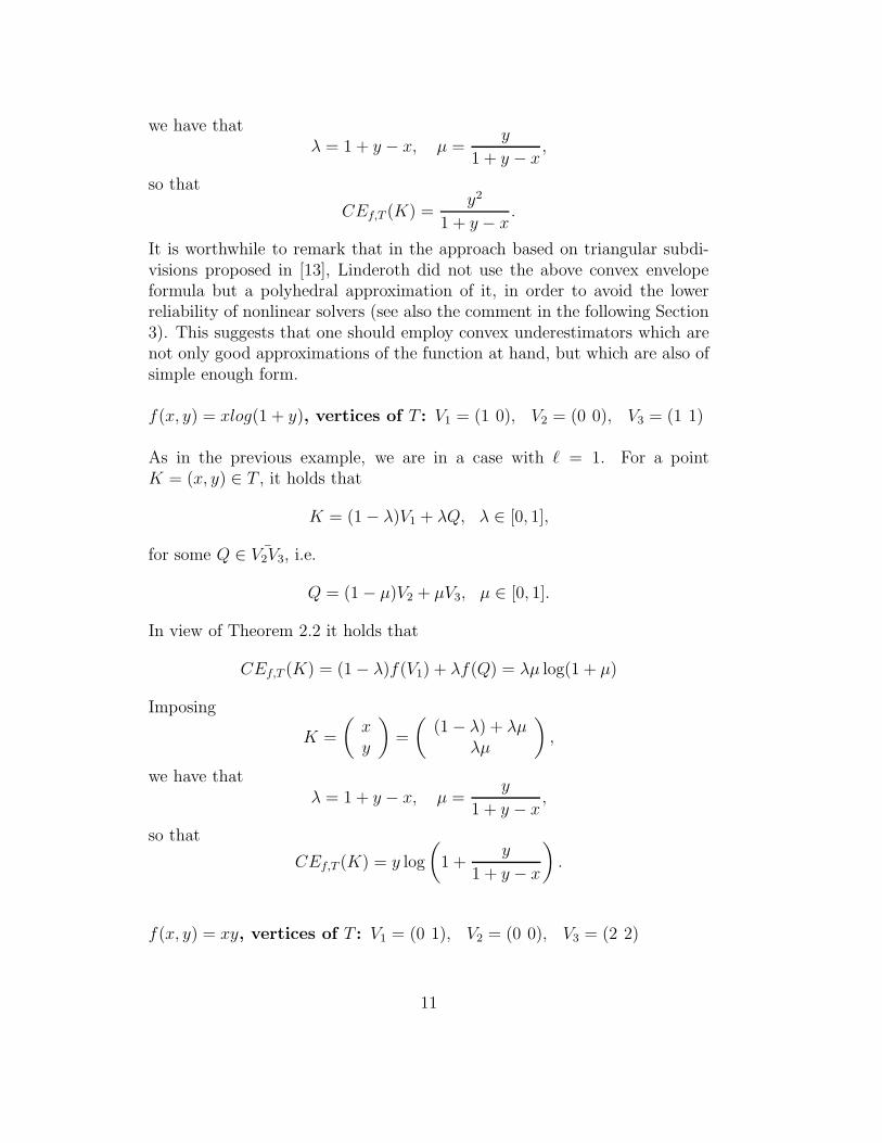
It is worthwhile to remark that in the approach based on triangular subdi-visions proposed in [13], Linderoth did not use the above convex envelopeformula but a polyhedral approximation of it, in order to avoid the lowerreliability of nonlinear solvers (see also the comment in the following Section3). This suggests that one should employ convex underestimators which arenot only good approximations of the function at hand, but which are also ofsimple enough form.
f(x, y) = xlog(1 + y), vertices of T : V1 = (1 0), V2 = (0 0), V3 = (1 1)
As in the previous example, we are in a case with ℓ = 1. For a pointK = (x, y) ∈ T , it holds that
K = (1 − λ)V1 + λQ, λ ∈ [0, 1],
for some Q ∈ ¯V2V3, i.e.
Q = (1 − µ)V2 + µV3, µ ∈ [0, 1].
In view of Theorem 2.2 it holds that
CEf,T (K) = (1 − λ)f(V1) + λf(Q) = λµ log(1 + µ)
Imposing
K =
(
xy
)
=
(
(1 − λ) + λµλµ
)
,
we have thatλ = 1 + y − x, µ =
y
1 + y − x,
so that
CEf,T (K) = y log
(
1 +y
1 + y − x
)
.
f(x, y) = xy, vertices of T : V1 = (0 1), V2 = (0 0), V3 = (2 2)
11

In this case ℓ = 2 holds. As seen in the proof of Theorem 2.2, we needto solve the following one-dimensional problem
minµ∈[λ1/(1−λ2),1]λ1
µf (µV1 + (1 − µ)V3) +
+
(
1 − λ1
µ
)
f
(
µλ2
µ − λ1
V2 +
(
1 − µλ2
µ − λ1
)
V3
)
,
whereλ1 = y − x, λ2 = 1 − y + x/2.
Elementary but quite tedious computations show that the result is the fol-lowing function
CEf,T (K) =
x2
1−y+x
√2
2x + y < 1
(3 − 2√
2)x2 + (6 − 4√
2)y2 + (6√
2 − 8)xy−−(4
√2 − 6)x + (4
√2 − 6)y otherwise
3 Convex envelope of bivariate functions over
polytopes
Let us consider a polytope P ⊂ R2 and a bivariate function f(x, y) satisfying
Conditions 1 and 2 of the previous section, with the triangle replaced bypolytope P . Moreover, we require that f ∈ C2. Note that these conditionsare satisfied by well known bivariate functions such as the bilinear one xyand the ratio one y/x (in the latter case we require that P lies in the interiorof the half-space x ≥ 0, or in the interior of the half-space x ≤ 0). We wouldlike to compute the value of the convex envelope of f over P at some point(x0, y0) ∈ P and to return a supporting hyperplane for the convex envelopeat that point. Knowledge of a supporting hyperplane is quite relevant forthe definition of a polyhedral convex underestimator of the convex envelope(maximum of the supporting hyperplanes at a finite set of points in P ).As remarked in [22], the use of polyhedral underestimators of the convexenvelope rather than the convex envelope itself is advisable in view of thehigher speed and stability of linear programming solvers with respect tononlinear ones.Among the different definitions of convex envelope of f over P , we also havethe one of pointwise supremum of the underestimating affine functions of fover P . Therefore, given some point (x0, y0) ∈ P , the value of the convexenvelope of f over P is given by the solution of the following optimization
12

problem in the three variables a, b and c with an infinite number of constraints
CEf,P (x0, y0) = max c
f(x, y) − [a(x − x0) + b(y − y0) + c] ≥ 0 ∀ (x, y) ∈ P.
The infinite number of constraints can be substituted by a single one involv-ing, however, a further optimization problem
CEf,P (x0, y0) = max c
min(x,y)∈P f(x, y) − [a(x − x0) + b(y − y0) + c] ≥ 0
The optimal solution (a∗, b∗, c∗) of this problem defines a supporting hyper-plane for the convex envelope of f over P at point (x0, y0).In view of Condition 1, the minimum of f(x, y)− [a(x − x0) + b(y − y0) + c]can not be attained (only) in the interior of P , and is always attained at avertex of P or along an edge of P such that the restriction of f along theedge is a convex (and not concave, i.e., not affine) function. Therefore, theconstraint
min(x,y)∈P
f(x, y) − [a(x − x0) + b(y − y0) + c] ≥ 0
can be rewritten as
f(xvi, yvi
) − [a(xvi− x0) + b(yvi
− y0) + c] ≥ 0 ∀ (xvi, yvi
) ∈ V (P )
min(x,y)∈ejf(x, y) − [a(x − x0) + b(y − y0) + c] ≥ 0 ∀ ej ∈ E ′(P )
where V (P ) denotes the vertex set of P , while E ′(P ) denotes the set of edgesof P along which f is strictly convex. More precisely, we can substitute therequirement for all the vertices in V (P ) with that for all the vertices inV ′(P ) ⊆ V (P ), where V ′(P ) is the set of vertices which do not belong toedges in E ′(P ). The constraints related to the vertices in V ′(P ) are simplelinear ones with respect to the unknowns a, b and c. Let us now considerthe constraints related to the edges in E ′(P ) which still involve optimizationproblems. For some ej ∈ E ′(P ), let us assume that the edge belongs to theline
y = mx + q.
Then, in view of the strict convexity assumption for f over the edge, thefollowing condition holds
f′′
ej(x) > 0 ∀ x ∈ [x
ej
1 , xej
2 ], (2)
where fej(x) = f(x, mx + q) denotes the restriction of f along the edge
ej ∈ E ′(P ), while xej
1 , xej
2 , xej
1 < xej
2 , denote the x-coordinates of the two
13

vertices in V (P ) defining ej . To be more precise, we should also consider thecase where the edge lies along a line x = β for some constant β, but this canbe dealt with in a completely analogous way. The constraint related to ej isthen
minx
ej1≤x≤x
ej2
fej(x) − [a(x − x0) + b(mx + q − y0) + c] ≥ 0 (3)
Let us denote by s(a, b) the minimum point of
fej(x) − (a + bm)x. (4)
We also allow for s(a, b) = +∞ (−∞) if the function is decreasing (increas-ing). In particular, note that if s(a, b) 6= ±∞, then
f ′ej
(s(a, b)) = a + bm. (5)
Therefore, the minimum point in (3) is
xej
1 if s(a, b) < xej
1
xej
2 if s(a, b) > xej
2
s(a, b) otherwise
with the minimum value
fej(x
ej
1 ) − (a + bm)xej
1 + ax0 + by0 − bq − c if s(a, b) < xej
1
fej(x
ej
2 ) − (a + bm)xej
2 + ax0 + by0 − bq − c if s(a, b) > xej
2
fej(s(a, b)) − (a + bm)s(a, b) + ax0 + by0 − bq − c otherwise
Taking into account that, in view of (2) the first derivative of fejis not de-
creasing along the interval [xej
1 , xej
2 ], then we can rewrite the above minimumvalue also as
fej(x
ej
1 ) − (a + bm)xej
1 + ax0 + by0 − bq − c if f ′ej
(xej
1 ) − (a + bm) ≥ 0
fej(x
ej
2 ) − (a + bm)xej
2 + ax0 + by0 − bq − c if f ′ej
(xej
2 ) − (a + bm) ≤ 0
fej(s(a, b)) − (a + bm)s(a, b) + ax0 + by0 − bq − c otherwise
Therefore, each constraint related to an edge ej ∈ E ′(P ) needs to be splitinto three different sets of constraints: one pair of linear constraints
fej(x
ej
1 ) − (a + bm)xej
1 + ax0 + by0 − bq − c ≥ 0
f ′ej
(xej
1 ) − (a + bm) ≥ 0
14

another pair of linear constraints
fej(x
ej
2 ) − (a + bm)xej
2 + ax0 + by0 − bq − c ≥ 0
f ′ej
(xej
2 ) − (a + bm) ≤ 0
and a third set with two linear constraints and a further constraint whosenature has to be clarified
fej(s(a, b)) − (a + bm)s(a, b) + ax0 + by0 − bq − c ≥ 0
f ′ej
(xej
1 ) − (a + bm) ≤ 0
f ′ej
(xej
2 ) − (a + bm) ≥ 0
Taking into account that such splitting into three groups of constraints needsto be done for all edges in E ′(P ), if we denote by t the cardinality of E ′(P ),we see that we need to solve (at most) 3t three-dimensional subproblems inorder to compute the value of the convex envelope of f over P at (x0, y0).What we still need to clarify is the nature of the constraints
fej(s(a, b)) − (a + bm)s(a, b) + ax0 + by0 − bq − c ≥ 0. (6)
What we will prove in the following theorem is that such constraints areconvex ones, so that all the subproblems to be solved in order to computethe convex envelope are convex ones.
Theorem 3.1 Under the given conditions, function
g(a, b) = fej(s(a, b)) − (a + bm)s(a, b)
is concave, so that constraint (6) is a convex one.
Proof. Throughout the proof we will omit the dependency of s form a, b.Let us compute the Hessian of g. We have that
gaa = f′′
ej(s)s2
a − 2sa + saa[f′ej
(s) − (a + bm)] = f′′
ej(s)s2
a − 2sa
where the last equality follows from (5). Analogously, we have that
gbb = f′′
ej(s)s2
b − 2msb + sbb[f′ej
(s) − (a + bm)] = f′′
ej(s)s2
b − 2msb,
gab = f′′
ej(s)sasb − msa − sb + sab[f
′ej
(s) − (a + bm)] = f′′
ej(s)sasb − msa − sb.
Then, the determinant of the Hessian is equal to
−(msa − sb).
15

It turns out that the determinant is null. Indeed, deriving both members of(5) with respect to a we get
f′′
ej(s)sa = 1, (7)
while deriving with respect to b we get
f′′
ej(s)sb = m,
so that sb = msa and the determinant is equal to 0. Then , in order to provethat the Hessian is semidefinite negative (i.e., that g is concave), we onlyneed to show that gaa, gbb ≤ 0. We notice that gaa (similar for gbb) is equal to
sa[f′′
ej(s)sa − 2],
but from (7) this is equal to −sa, so that
gaa ≤ 0 ⇔ sa ≥ 0.
Since, again from (7)
sa =1
f ′′
ej(s)
and since f′′
ej(s) > 0 in view of the strict convexity of fej
, we can concludethat sa is positive. 2
In order to illustrate the technique proposed in this section we consider thefollowing example.
f(x, y) = y/x, P triangle with vertices: V1 = (1 1), V2 = (1 2), V3 =(2 1)
There is a single edge, the one joining vertices V1 and V3, along which fis strictly convex. Therefore, given (x0, y0) ∈ P , we need to solve the threesubproblems
max c
c ≤ 2 − a + ax0 − 2b + 2y0
c ≤ 1 − a + ax0 − b + by0
a ≤ −1
max c
c ≤ 2 − a + ax0 − 2b + by0
c ≤ 12− 2a + ax0 − b + by0
a ≥ −1/4
16
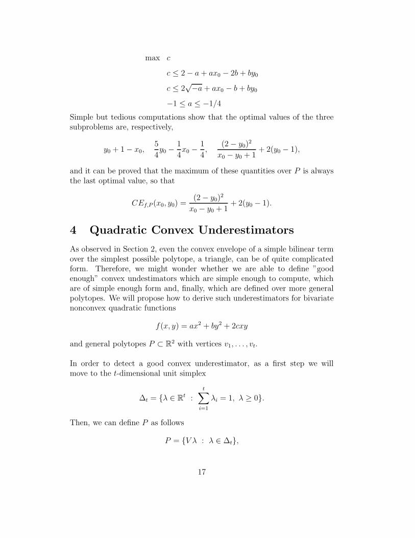
max c
c ≤ 2 − a + ax0 − 2b + by0
c ≤ 2√−a + ax0 − b + by0
−1 ≤ a ≤ −1/4
Simple but tedious computations show that the optimal values of the threesubproblems are, respectively,
y0 + 1 − x0,5
4y0 −
1
4x0 −
1
4,
(2 − y0)2
x0 − y0 + 1+ 2(y0 − 1),
and it can be proved that the maximum of these quantities over P is alwaysthe last optimal value, so that
CEf,P (x0, y0) =(2 − y0)
2
x0 − y0 + 1+ 2(y0 − 1).
4 Quadratic Convex Underestimators
As observed in Section 2, even the convex envelope of a simple bilinear termover the simplest possible polytope, a triangle, can be of quite complicatedform. Therefore, we might wonder whether we are able to define ”goodenough” convex undestimators which are simple enough to compute, whichare of simple enough form and, finally, which are defined over more generalpolytopes. We will propose how to derive such underestimators for bivariatenonconvex quadratic functions
f(x, y) = ax2 + by2 + 2cxy
and general polytopes P ⊂ R2 with vertices v1, . . . , vt.
In order to detect a good convex underestimator, as a first step we willmove to the t-dimensional unit simplex
∆t = {λ ∈ Rt :
t∑
i=1
λi = 1, λ ≥ 0}.
Then, we can define P as follows
P = {V λ : λ ∈ ∆t},
17

where V ∈ R2×t is the matrix whose columns are the coordinates of the
vertices of P . Next, we rewrite function f as follows
h(λ) = λT Qλ
where
Q = V T
(
a cc b
)
V.
A generic quadratic function over the t-dimensional unit simplex is the fol-lowing:
qS,c,v(λ) = λT [S + 1/2(ceT + ecT ) + vE]λ
where e ∈ Rt is the vector whose components are all equal to 1, while E ∈
Rt×t is the square matrix whose entries are all equal to 1. Note that over the
unit simplex ∆t this function is equal to
λT Sλ + cT λ + v.
In other words, we can always incorporate the linear terms in the matrix1/2(ceT + ecT ) and the constant ones in the matrix vE, in order to workwith a pure quadratic form with no linear and constant terms. Now, in orderto have a good convex underestimator we would like to choose S, c, v so thatqS,c,v is convex, underestimates h over the unit simplex ∆t (or, equivalently, fover P ) and the volume between h and qS,c,v is as small as possible. Basically,we aim at solving a problem with:
variables : S ∈ Rt×t, c ∈ Rt e v ∈ R;
constraints :
• convexity, i.e., S � O (S is a semidefinite matrix);
• qS,c,v underestimates h over ∆t. This means that
λT [Q − S − 1/2(ceT + ecT ) − vE]λ ≥ 0 ∀ λ ∈ ∆t
or, equivalently
Q − S − 1/2(ceT + ecT ) − vE ∈ Ct,
where Ct is the set of copositive matrices of order t.
objective : we would like to minimize the integral∫
∆t
λT [Q − S − 1/2(ceT + ecT ) − vE]λ.
18

The integral of a quadratic function over the unit simplex can be expressedin analytic form. It holds that the value of the integral defining our objectivefunction is
2
(t + 1)!E•[Q−S−1/2(ceT +ecT )−vE] =
2
(t + 1)!
t∑
i,j=1
[Q−S−1/2(ceT +ecT )−vE]ij .
Therefore, we are finally left with the following problem to be solved
min E • [Q − S − 1/2(ceT + ecT ) − vE]
S � O
Q − S − 1/2(ceT + ecT ) − vE ∈ Ct
(8)
The copositive constraint
Q − S − 1/2(ceT + ecT ) − vE ∈ Ct,
makes the problem a difficult one, but we might simplify it by substitutingthe copositive cone with the cone obtained as a sum of the semidefinite coneand the cone of nonnegative matrices, that is
Q − S − 1/2(ceT + ecT ) − vE ∈ Pt + Nt,
where Pt is the set of semidefinite matrices of order t, and Nt the set ofnonnegative matrices of order t. In particular, for t ≤ 4 the two cones areequivalent, while more generally it holds that
Pt + Nt ⊆ Ct
(see, e.g., [8] for an example of copositive matrix of order 5 which can notbe obtained as the sum of a semidefinite and a nonnegative matrix). Let usconsider the simplified problem
min E • [Q − S − 1/2(ceT + ecT ) − vE]
S � O
Q − S − 1/2(ceT + ecT ) − vE ∈ Pt + Nt
(9)
We can prove the following result.
Observation 4.1 The constraint
Q − S − 1/2(ceT + ecT ) − vE ∈ Pt + Nt
19

can be replaced by the constraint
Q − S − 1/2(ceT + ecT ) − vE ≥ O.
Moreover, for the optimal solution S∗, c∗, v∗ it holds that
qS∗,c∗,v∗(ei) = h(ei) ∀ i = 1, . . . , t.
where ei ∈ Rt is the i-th vertex of the unit simplex ∆t.
Proof. Notice that, given a feasible solution with
Q − S − 1/2(ceT + ecT ) − vE = P + N, P ∈ Pt, N ∈ Nt,
we can obtain a further feasible solution by substituting S with S ′ = S + P ,so that
Q − S ′ − 1/2(ceT + ecT ) − vE = N, N ∈ Nt.
If we compute the objective (the volume) in the new feasible solution, this isreduced, with respect to the starting feasible solution, by the quantity E •P ,which is certainly nonnegative in view of the semidefiniteness of E and P .Therefore, the new feasible solution is at least as good as the starting oneand we can substitute the constraint
Q − S − 1/2(ceT + ecT ) − vE ∈ Pt + Nt
with the following constraint
Q − S − 1/2(ceT + ecT ) − vE ≥ O.
Moreover, we also notice that
N ′ = N − Diag(N) ∈ Nt,
where Diag(N) is the diagonal matrix whose diagonal elements are equal tothose of matrix N . Then, we have that
Q − S ′ − Diag(N) − 1/2(ceT + ecT ) − vE = N ′, N ∈ Nt.
and setting S ′′ = S ′+Diag(N) (being N nonnegative, we have that Diag(N)is positive semidefinite) we still get a feasible solution with objective functionnot worse than the original one. In other words, we can impose the furtherconstraint
diag(Q) = diag(S + 1/2(ceT + ecT ) + vE),
20
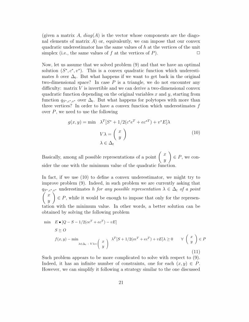
(given a matrix A, diag(A) is the vector whose components are the diago-nal elements of matrix A) or, equivalently, we can impose that our convexquadratic underestimator has the same values of h at the vertices of the unitsimplex (i.e., the same values of f at the vertices of P ). 2
Now, let us assume that we solved problem (9) and that we have an optimalsolution (S∗, c∗, v∗). This is a convex quadratic function which underesti-mates h over ∆t. But what happens if we want to get back in the originaltwo-dimensional space? In case P is a triangle, we do not encounter anydifficulty: matrix V is invertible and we can derive a two-dimensional convexquadratic function depending on the original variables x and y, starting fromfunction qS∗,c∗,v∗ over ∆t. But what happens for polytopes with more thanthree vertices? In order to have a convex function which underestimates fover P , we need to use the following
g(x, y) = min λT [S∗ + 1/2(c∗eT + ec∗T ) + v∗E]λ
V λ =
(
xy
)
λ ∈ ∆t
(10)
Basically, among all possible representations of a point
(
xy
)
∈ P , we con-
sider the one with the minimum value of the quadratic function.
In fact, if we use (10) to define a convex underestimator, we might try toimprove problem (9). Indeed, in such problem we are currently asking thatqS∗,c∗,v∗ underestimates h for any possible representation λ ∈ ∆t of a point(
xy
)
∈ P , while it would be enough to impose that only for the represen-
tation with the minimum value. In other words, a better solution can beobtained by solving the following problem
min E • [Q − S − 1/2(ceT + ecT ) − vE]
S � O
f(x, y) − minλ∈∆t : V λ=
xy
λT [S + 1/2(ceT + ecT ) + vE]λ ≥ 0 ∀(
xy
)
∈ P
(11)Such problem appears to be more complicated to solve with respect to (9).Indeed, it has an infinite number of constraints, one for each (x, y) ∈ P .However, we can simplify it following a strategy similar to the one discussed
21

in Section 3. First we observe that
f(x, y)− min
λ∈∆t : V λ=
xy
λT [S + 1/2(ceT + ecT ) + vE]λ ≥ 0 ∀(
xy
)
∈ P
is equivalent to
min(x,y)∈P
f(x, y) − min
λ∈∆t : V λ=
xy
λT [S + 1/2(ceT + ecT ) + vE]λ
≥ 0.
The optimal solution of the minimum problem on the left-hand side of thisinequality can not be a point in the interior int(P ) of P . Indeed
− min
λ∈∆t : V λ=
xy
λT [S + 1/2(ceT + ecT ) + vE]λ
is a concave function and if we consider (x, y) ∈ int(P ) we are always able tofind a direction along which also f(x, y) is concave (unless f is already convex,but in such case we do not need any convex underestimator) . Therefore,along the segment in P lying on the direction, we have a minimum value atone of the two extremes of the segment, that is along an edge of P . In acompletely analogous way, if along an edge we have that f is concave, thenthe minimum is attained at one of the two extremes of the edge. Therefore,we can finally rewrite the infinite set of constraints as follows
f(x, y)− min
λ∈∆t : V λ=
xy
λT [S+1/2(ceT +ecT )+vE]λ ≥ 0 ∀(
xy
)
∈ Xf(P )
where Xf(P ) is the generating set of the convex envelope of f over P , i.e., theset of edges of P along which f is not concave plus the vertices of P whichdo not belong to edges where f is not concave. The fact that we are able torestrict the attention to points along edges of P is an advantage. Indeed, fora point along an edge its representation through points λ ∈ ∆t is unique.
Now, let us recall the notation V ′(P ) and E ′(P ) introduced in Section 3.For the vertices in V ′(P ) we need to impose the linear constraints
qkk − skk − ck − v ≥ 0 ∀ vk ∈ V ′(P )
22
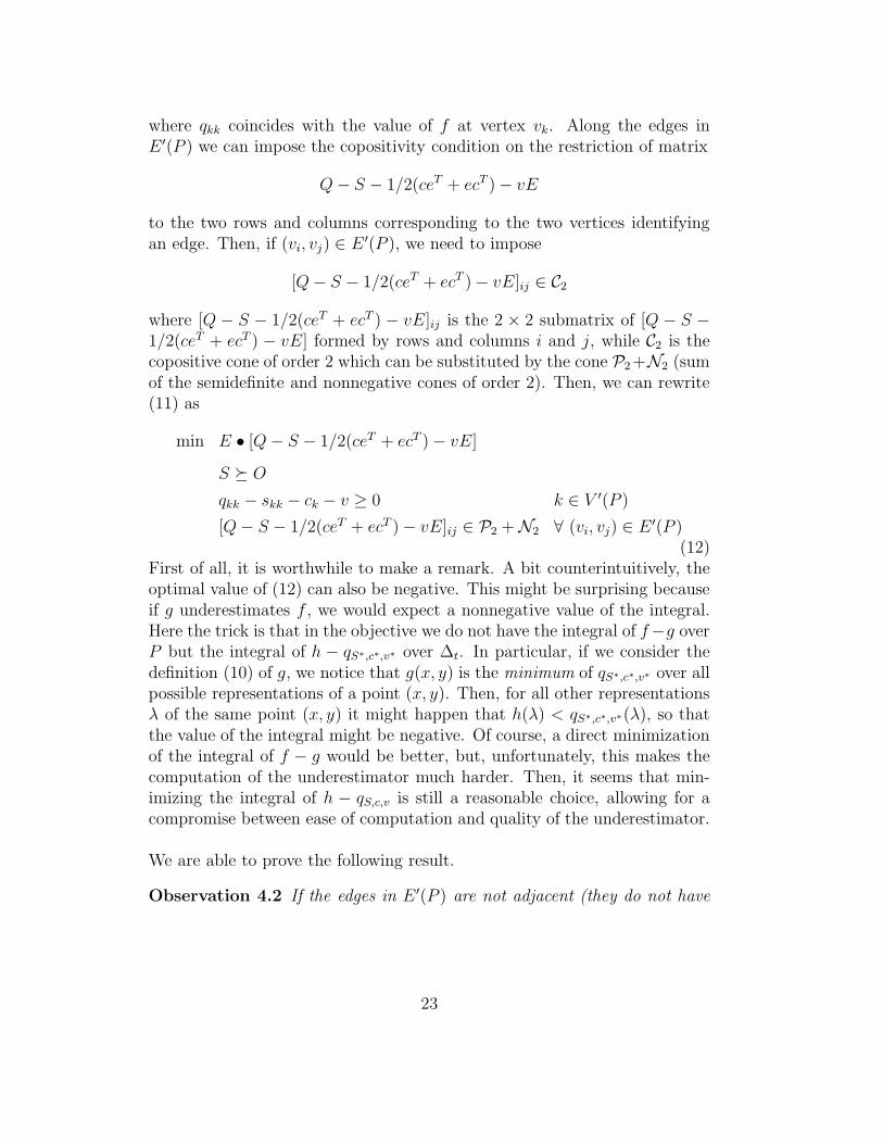
where qkk coincides with the value of f at vertex vk. Along the edges inE ′(P ) we can impose the copositivity condition on the restriction of matrix
Q − S − 1/2(ceT + ecT ) − vE
to the two rows and columns corresponding to the two vertices identifyingan edge. Then, if (vi, vj) ∈ E ′(P ), we need to impose
[Q − S − 1/2(ceT + ecT ) − vE]ij ∈ C2
where [Q − S − 1/2(ceT + ecT ) − vE]ij is the 2 × 2 submatrix of [Q − S −1/2(ceT + ecT ) − vE] formed by rows and columns i and j, while C2 is thecopositive cone of order 2 which can be substituted by the cone P2+N2 (sumof the semidefinite and nonnegative cones of order 2). Then, we can rewrite(11) as
min E • [Q − S − 1/2(ceT + ecT ) − vE]
S � O
qkk − skk − ck − v ≥ 0 k ∈ V ′(P )
[Q − S − 1/2(ceT + ecT ) − vE]ij ∈ P2 + N2 ∀ (vi, vj) ∈ E ′(P )(12)
First of all, it is worthwhile to make a remark. A bit counterintuitively, theoptimal value of (12) can also be negative. This might be surprising becauseif g underestimates f , we would expect a nonnegative value of the integral.Here the trick is that in the objective we do not have the integral of f−g overP but the integral of h − qS∗,c∗,v∗ over ∆t. In particular, if we consider thedefinition (10) of g, we notice that g(x, y) is the minimum of qS∗,c∗,v∗ over allpossible representations of a point (x, y). Then, for all other representationsλ of the same point (x, y) it might happen that h(λ) < qS∗,c∗,v∗(λ), so thatthe value of the integral might be negative. Of course, a direct minimizationof the integral of f − g would be better, but, unfortunately, this makes thecomputation of the underestimator much harder. Then, it seems that min-imizing the integral of h − qS,c,v is still a reasonable choice, allowing for acompromise between ease of computation and quality of the underestimator.
We are able to prove the following result.
Observation 4.2 If the edges in E ′(P ) are not adjacent (they do not have
23

common vertices), then we can rewrite (12) as follows
min E • [Q − S − 1/2(ceT + ecT ) − vE]
S � O
qii − sii − ci − v = 0 ∀ vi ∈ V (P )
qij − sij − 1/2(ci + cj) − v ≥ 0 ∀ (vi, vj) ∈ E ′(P )
(13)
Proof. The proof is similar to that of Observation 4.1. Let us denote by(S∗, c∗, v∗) an optimal solution of the problem. It holds that
[Q − S∗ − 1/2(c∗eT + ec∗T ) − v∗E]ij = Mij + Nij ∀ (vi, vj) ∈ E ′(P ),
where Mij ∈ P2 and Nij ∈ N2. If we consider the matrix M ′ij of order t which
is equal to Mij when restricted to rows and columns i and j and with all theother entries equal to 0, we have that M ′
ij ∈ Pt and we have a new optimalsolution if we set
S ′ = S∗ + M ′ij .
Then, we can substitute constraints
[Q − S − 1/2(ceT + ecT ) − vE]ij ∈ P2 + N2
with[Q − S − 1/2(ceT + ecT ) − vE]ij ∈ N2 ∀ (vi, vj) ∈ E ′(P ) (14)
With a similar proof, we can show that we can fix all the diagonal elementsof matrices Nij to 0. Therefore constraints (14) can be further rewritten asfollows
qii − sii − ci − v = 0 ∀ vi ∈ V (P ) \ V ′(P )qij − sij − 1/2(ci + cj) − v ≥ 0 ∀ (vi, vj) ∈ E ′(P )
Taking into account that the constraints
qkk − skk − ck − v ≥ 0 vk ∈ V ′(P )
can be substituted by equalities (a positive value of the left-hand side can besummed up to skk), we can finally rewrite (12) as (13). 2
The following easy observations also hold.
Observation 4.3 Under the assumptions of Observation 4.2, the returnedconvex underestimator is equal to f at the vertices of P .
24

Proof. This is an immediate consequence of the equality constraints
qii − sii − ci − v = 0 ∀ vi ∈ V (P ).
2
Observation 4.4 For the polyhedral cases, i.e., those for which E ′(P ) = ∅,the returned convex underestimators is the convex envelope of f over P .
Proof. We first observe that in this case
S = O, ci = qii ∀ vi ∈ V (P ), v = 0
is a feasible solution for (13). Moreover, for any other feasible solution(S, c, v) of (13) it holds, in view of convexity, that
qS,c,v(λ) = (∑t
i=1 λiei)T S(
∑ti=1 λiei) + c(
∑ti=1 λiei) + v
≤ ∑ti=1 λi(e
Ti Sei + cei + v) =
∑ti=1 λi(sii + ci + v) =
∑ti=1 λiqii = qS,c,v(λ),
i.e., (S, c, v) is also optimal for (13). The corresponding function
g(x, y) = min∑t
i=1 qiiλi
V λ =
(
xy
)
λ ∈ ∆t
is exactly the convex envelope. 2
Now, let us consider non polyhedral cases. We might wonder whether thereturned solution is always at least as good as the convex envelope over thesmallest box B ⊇ P . The following example shows that this is not alwaysthe case.
Example 4.1 Let f(x, y) = xy and T be the triangle with vertices (0, 0),(0, 1) and (1, 1). The smallest box B containing T is the unit square, overwhich the convex envelope is
h(x, y) = max{0, x + y − 1}.With some computations we have that the solution of (13), when expressedin terms of the original variables x, y is the function
g(x, y) =1
2x2 +
1
4y2 +
1
4xy − 1
4y +
1
4x.
Even if the volume between xy and g over T is lower than that between xy andh (3/96 the former, 1/24 the latter), it does not hold that g(x, y) ≤ h(x, y)∀ (x, y) ∈ T (e.g., this does not hold for x = 0, y = 1).
25

However, in such cases we can define a new convex underestimator ℓ takingthe maximum between h and g. In the example we have that
ℓ(x, y) = max
{
0, x + y − 1,1
2x2 +
1
4y2 +
1
4xy − 1
4y +
1
4x
}
.
We conclude this section remarking that a similar development could beextended to bivariate polynomial functions satisfying Conditions 1 and 2 ofSection 2. Indeed, in such cases we might exploit along each edge in E ′(P )the semidefinite representation of nonnegative one-dimensional polynomials(see, e.g., [5])
5 Conclusions
In this paper we discussed convex underestimators for functions over two-dimensional polytopes. In Section 2 we proposed a method to derive theconvex envelope of bivariate functions, satisfying three conditions, over thesimplest two-dimensional polytopes: triangles. In Section 3 we have shownthat the computation of the value at some point of the convex envelope overa general two-dimensional polytope, together with a supporting hyperplaneof the convex envelope at that point, requires the solution of some three-dimensional convex subproblems. Having remarked that the convex envelopemight be of quite complicated form (even over triangles), in Section 4 weproposed a method, based on the solution of a semidefinite program, toderive convex underestimators for bivariate quadratic functions over generaltwo-dimensional polytopes.
References
[1] C. S. Adjiman, I. P. Androulakis, C. A. Floudas, A global optimiza-tion method, α-BB, for general twice-differentiable constrained NLPs -II. Implementation and Computational Results, Comp. Chem. Eng., 22:1159-1179 (1998)
[2] F. A. Al-Khayyal, J. E. Falk, Jointly constrained biconvex programming,Mathematics of Operations Research, 8: 273-286 (1983)
[3] K. M. Anstreicher, S. Burer, Computable representations for convex hullsof low-dimensional quadratic forms, to appear in Mathematical Program-ming (2010)
26

[4] H. P. Benson, On the construction of convex and concave envelope formu-las for bilinear and fractional functions on quadrilaterals, ComputationalOptimization and Applications, 27: 5-22 (2004)
[5] L. Brickman, L. Steinberg, On nonnegative polynomials, The AmericanMathematical Monthly, 69: 218-221 (1962)
[6] Y. Crama, Recognition problems for polynomials in 0-1 variables, Math-ematical Programming, 44: 139-155 (1989)
[7] Y. Crama, Concave extensions for nonlinear 0-1 maximization problems,Mathematical Programming, 61: 53-60 (1993)
[8] P. H. Diananda, On non-negative forms in real variables some or all ofwhich are non-negative, Proc. Cambridge Philos. Soc. , 58: 17-25 (1967).
[9] R. Horst, H. Tuy, Global optimization: deterministic approaches, SpringerVerlag, Berlin, 3rd edition (1996).
[10] T. Kuno, A branch-and-bound algorithm for maximizing the sum ofseveral linear ratios, Journal of Global Optimization, 22: 155-174 (2002)
[11] M. Jach, D. Michaels, R. Weismantel, The Convex Envelope of (n–1)-Convex Functions, SIAM Journal on Optimization, 19(3): 1451-1466(2008)
[12] L. Liberti, C. C. Pantelides, Convex Envelopes of Monomials of OddDegree, Journal of Global Optimization, 25(2): 157-168 (2003)
[13] J. Linderoth, A simplicial branch-and-bound algorithm for solvingquadratically constrained quadratic programs, Mathematical Program-ming, 103: 251-282 (2005)
[14] G. P. McCormick, Computability of global solutions to factorable non-convex programs – Part I – Convex underestimating problems, Mathe-matical Programming, 10:147–175 (1976).
[15] C.A. Meyer, C.A. Floudas, Convex envelopes for edge-concave functions.Mathematical Programming, 103:207–224 (2005).
[16] A. Rikun,A convex envelope formula for multilinear functions, Journalof Global Optimization, 10: 425-437 (1997)
[17] H. S. Ryoo, N. V. Sahinidis,Analysis of bounds for multilinear functions,Journal of Global Optimization, 19: 403-424 (2001)
27

[18] H. D. Sherali, A. Alameddine, An explicit characterization of the convexenvelope of a bivariate bilinear function over special polytopes, Annalsof Operations Research, 27: 197-210 (1992).
[19] H. D. Sherali, Convex envelopes of multilinear functions over a unithypercube and over special discrete sets, Acta Mathematica Vietnamica,22: 245-270 (1997)
[20] M. Tawarmalani, N. V. Sahinidis, Semidefinite relaxations of fractionalprograms via novel convexification techniques, Journal of Global Opti-mization, 20: 137-158 (2001).
[21] M. Tawarmalani, N. V. Sahinidis, Convex extensions and envelopes oflower semicontinuous functions, Mathematical Programming, 93: 247-263(2002)
[22] M. Tawarmalani, N. V. Sahinidis, A polyhedral branch-and-cut ap-proach to global optimization, Mathematical Programming, 103: 225-249(2005)
[23] F. Tardella. On the existence of polyhedral convex envelopes, inC.A. Floudas, P.M. Pardalos (eds.), Frontiers in Global Optimization,Dordrecht, Kluwer Academic Publishers, 563-574 (2003).
[24] J.M. Zamora, I.E. Grossmann, A Branch and Contract algorithm forproblems with concave univariate, bilinear and linear fractional terms,Journal of Global Optimization, 14, 217-249 (1999).
28