On computationally adjusting the Hill equation of adsorption

104

On Computationally Adjusting the Hill Equation of Adsorption

Joaquin Cortes, Heinrich Puschmann, and Eliana Valencia Universidad de Chile, Facultud de Ciencias Fisicas y Matematicas, Casilla 2777, Santiago 3, Chile Received 4 October 1982; accepted 25 July 1983

We discuss the implementation and computational efficiency of one approach to adjusting the Hill equation of adsorption to a set of empirical data, pointing out some aspects that seem to be valid in the general case. The approach consists basically of minimizing squares of deviations of the adsorbed amounts, which are numerically computed in terms of the empirical pressures and the parameters. Hill’s equation is dealt with as a prototype of nonlinear equations seldom used by chemists because none of their variables can be set free.

I. INTRODUCTION

Two aspects will be of interest in this article. First, we discuss an approach of computing least squares when adjusting a nonlinear equation to a set of empirical data, and the variable whose square deviations we wish to minimize cannot explicitly be expressed in terms of the rest. Our approach consists in performing an unconstrained minimization over the domain of the parameters, and at each of its iterations numerically compute the deviated variable from the other variables and the parameters. In our case, such a treatment yielded very satisfactory results and proved to be much more efficient than casting the problem into a constrained minimization framework.

Secondly, we apply the above approach to Hill’s equation for an adsorption isothenn1v2 and discuss the problems that had to be dealt with in this specific case. We hope that Hill’s equation provides a useful illustration of the general case, taking it as a prototype of nonlinear equations seldom used by chemists because of their mathema tical complexity .

In section I1 we review several ways of setting up the least squares problem to adjust a physical equation, as well as some simplifications to re- duce the computational complexity of the minimization. In section I11 we discuss the computational approach, and in section IV we apply it to the Hill equation. In section V some empirical results of processing laboratory data are summed up. Finally, section VI is devoted to miscella- neous remarks about related models which we did not implement.

11. THE LEAST SQUARES APPROACH

The importance of using convenient criteria for adjusting experimental adsorption data to theoretical models has been discussed in some of our recent publication^?-^ The first one explains a number of discrepancies about the parameters of Anderson’s adsorption equation 6, by showing that those discrepancies disappear if one additional significant figure is considered in one of the parameters. The second article analyzed the applicability range of the Frenkel-Halsey-Hill (FHH) equation,8-I0 and the third one does simi- larly with the equation of Hill-de Boer.’.’l

In all these articles, the adjustment of theoretical models to sets of experimental data was done using a least squares method. This approach is widely used by chemists when the equations describing the theoretical model can be made linear, and a least squares straight line can be searched for. If this is not the case, the problem becomes one of nonlinear regression, showing new numerical and computational aspects.

Let us assume that a theoretical model can be represented by an equation that relates two variables, u and o, and depends on a set of m parameters represented by the vector K =

( 4 , . * ,Km):

+(u, 0, K ) = 0, aj < KJ < bj (1) + will usually have continuous derivatives within its range of application. Let us consider, too, that we have a set of n pairs of data or “experimental points”

Journal of Computational Chemistry, Vol. 5, No. 1, 104-112 (1984) 0 1984 by John Wiley & Sons, Inc. CCC 0192-8651/84/0100104-09$04.00

Adjusting the Hill Equation 105

Assuming that the model of eq. (1) is true, we wish to find values k of the parameters that are optimal in supplying the required information from the experimental system. According to the least squares approach, those optimal parameters are given by the following constrained minimization problem:

Minimize [ ( ui ; iii)’ + ( vi ; i&)’] (3a) i = 1

Ui, ui, K

subject to

+ ( u , , u , , K ) = 0, i = 1 ,..., n (3b)

aj < K j < bj, j = 1, ..., m (3c)

The statistical weights a, and T~ in the objective function (3a) should ideally be chosen propor- tional to the variances of the errors of measure- ment. If we assume that the n experiments are statistically independent with normally distrib- uted errors, then the criterion of least squares is a consequence of the principle of maximum like- lihood. This criterion can certainly be gener- alized to more than two variables.

The minimization problem (3) has 2n + m variables and m equality constraints. In order to simplify it, additional assumptions are very often made. We shall suppose that:

All experimental error is assigned to only one of the variables, i.e. 7i = 0, (4) i =1, ..., n

This is a very daring assumption, and we intend no validation; however, it reduces the number of minimization variables to almost one-half. The problem becomes

2 Minimize t (Ui “ i )

ui , K i = 1

subject to

+ ( u i , u i , K ) = 0, i = 1 ,..., n (5b)

aj < K j < bj, j = 1,. . . ,m (5c)

A further simplification takes place under the following assumption:

There is a closed algebraic expression for u in terms of v and K , i.e. an explicit function f such that +( f ( u, K ) , v , K ) = 0 (6)

This is an assumption of the model rather than

of the experiment. If (4) and (6) hold true, the problem becomes

subject to

aj < K j < bj, j = 1,. . . ,m (7b)

Therefore, only parameter variables and no equality constraints are left.

If we do not want to make use of assumption (4), assumption (6) may be substituted by a slightly weaker version:

There are closed algebraic expressions for u and o in terms of a dummy variable t and K , i.e. explicit functions g and h such that +(g(t, K), h(t, K), K ) = 0

(6’)

A pair of expressions like g(t, K), h(t, K ) is called a parametrization of +. The dummy variable t is called a “parameter” in other contexts, but to keep things apart we shall not do so here. The minimization problem now has n + m variables and no equality constraints:

subject to

aj < K j < bj, j = 1, ..., m (8b)

This case is presumably not very important; we include it here because the Hill equation admits a parametrization.

There is abundant literature on computational methods for nonlinear least squares fitting; see ref. 12 for a critical overview and refs. 13-15 for some specific methods. If the problem is linear in some of its variables, an approach as in refs. 16 and 17 can be used. All the above, however, do not admit constraints, thus implicitly making assumptions (6) or (6’). In this work we shall discuss problem (9, thus maintaining assumption (4), while dropping (6) or (6’). To the authors knowledge, there is no publication dealing with that case.

106 CortQ, Puschmann, and Valencia

111. DECOMPOSITION OF THE PROBLEM

Minimization problem (5) contains two kinds of constraints: separable equality constraints (5b) and nonactive inequality bounds (5c). We shall exploit both of these features when separately dealing with each kind.

One way to handle equality constraints with special ease is by means of Lagrange multipliers. The Augmented Lagrangian solves the constrained minimization problem by iteratively approximating its Lagrange multipliers to their true values. At a given iteration t , an unconstrained problem (7) with tentative multipliers y: is solved, and its solution uf, K t is used to update the multipliers:

subject to aj < K j < bj, j = 1, ..., rn (9b)

,,+I = y; + w+(u;, q, K t )

Here w > 0 (typically lo3 I w I lo5) is an arbi- trary constant, whose task is to keep the intermediate solutions u:, K t within a neighborhood of the true solution. The constraints (9b), which are nonactive at the true solution, will remain nonactive at intermediate optima uf, K if w > 0 is large enough. The whole process is stopped when the ly;+' - y,"l are smaller than a given tolerance A.

The unconstrained problem (9), for its part, is also solved iteratively. Methods for doing so can be found in refs. 12,18,23, and many others. Not all of those, though, will be useful for implicitly handling the nonactive constraints (5c) or (9b). In order to discriminate between them, let us have a look at their general framework.

Let F(x) , x = (xl,. . . ,xn) be a function having continuous partial derivatives F'(x) = ( F { ( x ) ,..., Fi(x)) and let xt = (x4 ,..., xk), the current searching point at iteration t. Most algorithms will then somehow determine a search direction d = ( d;, . . . , d i ) such that

such that F(xt + adt ) decreases at a smart rate

in a neighborhood of a > 0. Usually d t points towards the minimum of an approximated version or function model of F ( x ) at xt, but we shall not go into more details. After the direction choice was made, a line search is performed, yielding an at > 0 such that the decrease of F(xt + adt) is large enough,

F(xt + atdt) < F(xt) (1W

Finally, a new search point xt+' = xt + atdt is defined and a new iteration is started. For suitable policies of direction choice and line search, it can be shown that

If the sequence xl, x 2 , - - 7 converges towards X, then x is a stationary point, i.e. F'(Z) = 0

(12)

Proofs would go along the lines of ref. 22. We observe that a stationary point need not be a local minimum. However, if X is not a minimum and the Hessian matrix F"(x) is nonsingular, then it is almost impossible that xl, x2, * . . converges to Z.22 On the other hand, the xf might increase without bound and not converge, even if there is a local minimum available. If F(x) has continuous second derivatives in a neighborhood of the convergence point, a good algorithm should produce superlinear convergence, meaning that the more we approach Z, the faster is the relative progress we make. The process is stopped when the IxE+' - xi1 are smaller than a given tolerance 6 << A.

When minimizing F(x) subject to nonactive constraints, as ai < x i < b,, we would like to handle these constraints substituting F ( x ) by a very large constant, whenever it violates the constraints.

if ai < x i < bi, i = 1, ..., n M >> 0 otherwise

Note that the derivatives of P are undefined for any x that violates the constraints. Thus, we need a feasible starting point ai < x: < bi, and an algorithm that satisfies the following extra requirement:

The line search determining at > 0 does not make use of derivatives F'(xt + adt ) for a > 0

(14)

Quite a number of algorithms providing superlinear convergence need a line search that satisfies


the extra condition that F'(xt + atdt) be or- thogonal to dt. It is very time-consuming to achieve that, if we are not allowed to evaluate F'(xt + adt ) as a consequence of (14). Moreover, such an extra condition can only be satisfied approximately, leaving the task of deciding on a suitable accuracy. Therefore, we wish to use a direction choice that leads to superlinear convergence independently of F '( x t + ') being ortho- gonal to xt+' - d. Appropriate choices are described in refs. 23-25. They can readily be combined with a line search proposed by Armijo,26*23 which is mentioned less often than it deserves. In our work, we have used ref. 23 throughout.

Thus, we may solve our problem by performing a sequence of unconstrained minimizations, typically 4 to 6. There is, however, an alternative approach. We may do a single unconstrained minimization, as if dealing with problem (7) instead of problem (5). Of course, there is no algebraic expression u = f (u , K ) as in problem (7); but we may use the equality constraints +( u, B, K ) = 0 in order to numerically compute u = f (a , K ) for each B and each feasible K that show up during the process. For a K out of bounds we generate an artificially large devia- tion:

= f ( u , K ) i f u j < K < b j , j=1 , ..., m M B O otherwise

u = {

Once we know, for feasible K , an u = f ( 8 , K ) such that +(u, 3, K ) = 0, we do also know its derivatives because of the formula

If K is out of bounds, no derivatives are available, and we have to rely again on property (14) of the unconstrained minimization algorithm.

If the equation solving approach is to be used for minimizing (5), the precision for numerically computing u = f ( B, K ) has to be significantly higher than the unconstrained minimization tolerance 6, since otherwise we may not reason- ably expect the termination criterion IK;+' - Kjl < 6 ever to be fulfilled. Moreover, the numerical evaluation of u = f ( B, K ) will typically be performed hundreds of times, and the algorithm used for solving $(u, 6, K ) = 0 will have to be not only very precise, but also very reliable. If 500 evaluations are needed for one

adjustment, a subroutine that worked 99% of the time would be of no use at all, since the overall method would work less than 1% of the time. Methods for solving a nonlinear equation are widely kn0wn,27-29 but they have to be carefully implemented in order to be both efficient and reliable. Each model I$( u, u, K ) = 0 should be studied separately and use be made of its specific properties. In the next section, we describe a specialization of the Newton-Raphson algorithm to the equation of Hill, which has proved to be very successful.

When comparing the Augmented Lagrangian approach with the equation solving approach for our case, the second turned out to be more reliable than the first and more than 10 times as fast. We believe that so big a difference does not depend just on the Hill equation and will probably carry over to other models. Therefore, a serious attempt should be made in designing a reliable algorithm that solves +( u, u, K ) for the variable whose squared deviations we wish to minimize; it will probably be worth the effort. The reason for the increased efficiency seems to be that the equality constraints (5b) are separable in the sense that each one depends only on one of the variables ul,. . . ,un. The Augmented Lagrangian approach ignores that property, and we should always bear in mind that the computational effort for either minimizing a function or solving a system of equations is heavily depen- dent on the number of variables. We can also visualize the equation solving approach as a case of consecutive regression, with a philosophy similar to refs. 16, 17.

We wish to emphasize that we made no exhaustive comparison among all available methods, but quit the analysis after obtaining satisfactory results.

IV. NUMERICAL TREATMENT OF THE HILL EQUATION

In 1946, Hill' developed a statistical mechani- cal model for multimolecular adsorption, assuming that the first adsorbed layer behaves as a bidimensional van der Waals gas. The expression for the adsorption isotherm for this model is

K16(1 - x ) 2 6(l - x) - x = [l - 6(l - x)] exp[ [l - 6( l - x)]

-K26(l - x)] (17a)

108 CortQ, Puschmann, and Valencia

0 < x < 1, 8 > 0, K , > 0, K , < 6.75

(17b)

where 8 = V,/V, is the fraction of covered surface (with V, the amount of adsorbed gas per gram of solid and V, the amount corresponding to a monolayer) and x is the relative pressure P/Po (with P representing the equilibrium pressure and Po the saturation pressure of the adsorbate). Parameter K , depends on the properties of the adsorbate, and K, on those of the gassolid system through the heat of adsorption. As x + 0, 8 4 0, the Hill equation (H) collapses with the so called Hill-de Boer equation (HDB), which was derived independently by de Boer'' from Gibbs' equation. Its expression is

x > 0, 0 < 8 < 1, K, > 0, K, < 6.75

(18b)

We observe that for neither equation there is a closed algebraic expression of 8 in terms of x, K,, K,. Although HDB can be used to minimize the square deviations of x, this is valid only for small x, 8 , and for errors attached to the pressure variable x.

Among all models of physisorption isotherms, that of Hill is one of the less used by experimental workers, presumably because of its mathematical complexity. In spite of its limitations, it has recently been considered anew.2 It therefore seems worthwhile promoting a more widespread use of i t in interpreting experimental systems, thereby clarifying some of its virtues and limitations.

Let us simplify (17) by defining a new set of coordinates as follows:

Q = Kl(l - X)/X

u = [I - 8( i - x)] / [e( i - x)] (19)

x = Ki/(Ki + Q) 8 = (Q + Ki)/[Q(U + 111 (20)

Substituting (20) into (17) yields the equation

Q = Uexp[ K 2 / ( U + 1) - l /U] (21a)

Q > 0, U > 0, K, < 6.75 (21b)

where U moves from 00 to 0 as Q moves from 00

to 0, or as x moves from 0 to 1. We wish to

compute U for given Q and K,, where condition K , < 6.75 makes sure that such U is well defined.

Equation (21) can be given the form

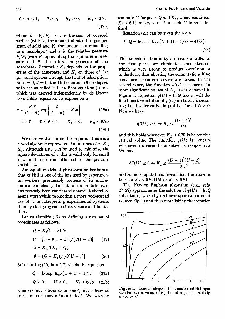
l n Q = l n U + K , / ( U + l ) - l / U = $ ( U )

(22)

This transformation is by no means a trifle. In the first place, we eliminate exponentiation, which is very prone to produce overflows or underflows, thus aborting the computations if no convenient countermeasures are taken. In the second place, the function + ( U ) is concave for most significant values of K,, as is depicted in Figure 1. Equation + ( U ) = In Q has a well defined positive solution if +( U ) is strictly increas- ing; i.e., its derivative is positive for all U > 0. Now we have

and this holds whenever K , < 6.75 is below this critical value. The function + ( U ) is concave whenever its second derivative is nonpositive. We have

(U + I ) ~ ( u + 2) 2u3

$" (U) I 0 a K , I

and some computations reveal that the above is true for K , I 5.841151 or K, I 5.84

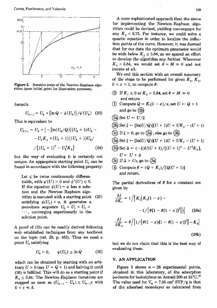
The Newton-Raphson algorithm (e.g., refs. 27-29) approximates the solution of +( U ) = In Q substituting +( U ) by its linear approximation at U, (see Fig. 2) and thus establishing the iteration

Iy'u'I

/

/

2.0-

1.5-

2 4 I I

6 g u

Figure 1. Concave shape of the transformed Hill equation for several values of K,. Inflection points are desig- nated by 0.

Cortk, Puschmann, and Valencia 109

uI'u'/

Figure 2. Iterative steps of the Newton-Raphson algorithm (poor initial point for illustration purposes).

formula

U,+i = u, + I1.Q - 4(u,)I/4'(u,) (23)

This is equivalent to

u,+i = U, + { - [ln(U,/Q)I (u, + l>u, - - UkK, +(U, + l))(U, + 1 ) W

/( (U, + - U 3 2 ) (24)

but the way of evaluating i t is certainly not unique. An appropriate starting point U, can be found in accordance with the following property:

Let I) be twice continuously differen- tiable, with #'(U) > 0 and $"(U) I 0. If the equation +(U) = a has a solution and the Newton-Raphson algorithm is executed with a starting point (25) satisfying I)(Uo) < a, it generates a monotone sequence V, < U, < U, < - - , converging superlinearly to the solution point.

A proof of (25) can be readily derived following well established techniques from any textbook on the topic (ref. 29, p. 453). Thus we need a point U, satisfying

uo > 0, I)(Uo) I h Q (26)

which can be obtained by starting with an arbi- trary U > 0 (say U = Q + 1) and halving it until (26) is fulfilled. This will do as a starting point if K , 5 5.84. The Newton-Raphson iterations are stopped as soon as (U,,, - U,) I U k + l ~ with O < E K 6 .

A more sophisticated approach than the above for implementing the Newton-Raphson algorithm could be devised, yielding convergence for any K , < 6.75. For instance, we could solve a quartic equation in order to localize the inflection points of the curve. However, it was deemed that for our data the optimum parameter would be wide below K , I 5.84, so we spared an effort to develop the algorithm any further. Whenever K , > 5.84, we would set 8 = M >> 0 and not iterate at all.

We end this section with an overall summary of the steps to be performed for given K , , K , , 0 < x < 1, to compute 8:

@ IfK, I OorK, > 5.84,setO = M >> 0 and return

0 Compute Q = K,(1 - x)/x, set U + Q + 1 and go to @

@Set u + ~ / 2

@Set Z + [h(U/Q)](U + 1)U + U K , - (U + 1)

@ Set Z 6 [ln(U/Q)](U + 1)U + UK, - (U + 1) @Set A + ( -<)U(U + l)/[(U + 1)3 - U 2 K , ] ,

U + - U + A @ I f A > UE,goto@ @ Compute8 = ( Q + K1)/[Q(U + l ) ]

and return.

The partial derivatives of 8 for x constant are given by

- l / [ O ( l - 8(1 - x))'])] (28a)

but we do not claim that this is the best way of evaluating them.

V. AN APPLICATION

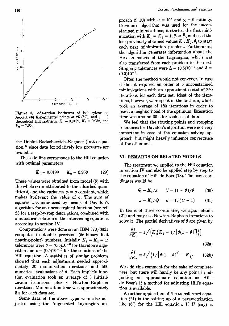
Figure 3 shows n = 26 experimental points, obtained in this laboratory, of the adsorption isotherm for isobutylene on Aerosil200 a t 25°C.30 The value used for V, = 7.05 cm3 STP/g is that of the adsorbed monolayer as calculated from

110 Cortbs, Puschmann, and Valencia

PRESSURE [ T o r t I

Figure 3. Adsorption isotherms of isobutylene on Aerosil. (0) Experimental points at 25 ("C), and (--) theoretical Hill isotherm. K , = 0.0199, K , = 0.958, and V, = 7.05.

the Dubini-Radushkevich-Kaganer ( DRK) equa- t i ~ n , ~ , since data for relatively low pressures are available.

The solid line corresponds to the Hill equation with optimal parameters

K, = 0.0199 K, = 0.958 (29)

These values were obtained from model (5) with the whole error attributed to the adsorbed quan- tities @, and the variances a, = u constant, which makes irrelevant the value of (I. The sum of squares was minimized by means of Davidon's algorithm for an unconstrained function (see ref. 23 for a step-by-step description), combined with a numerical solution of the intervening equations according to section IV.

Computations were done on an IBM 370/3031 computer in double precision (56-binary-digit floating-point) numbers. Initially K, = K, = 1; tolerances were S = (O.5)1Op6 for Davidon's algorithm and E = (0.5)10-10 for the solutions of the Hill equation. A statistics of similar problems showed that each adjustment needed approximately 20 minimization iterations and 500 numerical evaluations of 8. Each implicit function evaluation took an average of 3 initiali- zation iterations plus 6 Newton-Raphson iterations. Minimization time was approximately 2 s for each data set.

Some data of the above type were also ad- justed using the Augmented Lagrangian ap-

proach (9,lO) with ~3 = lo5 and yi = 0 initially. Davidon's algorithm was used for the unconstrained minimizations; it started the first minimization with K , = K, = 1, @, = ei, and used the last previously obtained values K,, K,, Bi to start each next minimization problem. Furthermore, the algorithm generates information about the Hessian matrix of the Lagrangian, which was also transferred from each problem to the next. Stopping tolerances were A = (0.5)10-4 and S =

(O.5)1Op6. Often the method would not converge. In case

it did, it required an order of 5 unconstrained minimizations with an approximate total of 250 iterations for each data set. Most of the iterations, however, were spent in the first run, which took an average of 180 iterations in order to reach a neighborhood of the optimum. Execution time was around 30 s for each set of data.

We feel that the starting points and stopping tolerances for Davidon's algorithm were not very important in case of the equation solving approach, but might heavily influence convergence of the other one.

VI. REMARKS ON RELATED MODELS

The treatment we applied to the Hill equation in section IV can also be applied step by step to the equation of Hill-de Boer (18). The new coordinates would be

x = Kl/Q 8 = 1/(U + 1) (31)

In terms of these coordinates, we again obtain (21) and may use Newton-Raphson iterations to solve it. The partial derivatives of 8 are given by

We add this comment for the sake of complete- ness, but there will hardly be any point in adjusting an approximate equation as Hill- de Boer's if a method for adjusting Hill's equation is available.

A further application of the transformed equation (21) is the setting up of a parametrization like (6') for the Hill equation. If U (say) is


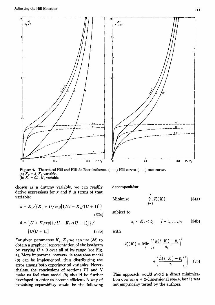
Figure 4. Theoretical Hill and HiKde-Boer isotherms. (--) Hill curves, (- - - -) HDB curves. (a) K , = 3, K , variable. (b) K , = 0.1, K , variable.

chosen as a dummy variable, we can readily derive expressions for x and 0 in terms of that variable:

x = K l / { K , + U/exp[ 1/U - K , / ( u + I)] } (334

[wJ+ 01 (33b)

6 = { U + K,exp[l/U- K 2 / ( U + l)]}/

For given parameters K,, K , we can use (33) to obtain a graphical representation of the isotherm by varying U > 0 over all of its range (see Fig. 4). More important, however, is that that model (8) can be implemented, thus distributing the error among both experimental variables. Never- theless, the conclusions of sections 111 and V make us feel that model (8) should be further developed in order to become efficient. A way of exploiting separability would be the following

decomposition:

Minimize i F , ( K ) i = l

subject to

a j < K j < bj j = 1, ..., m with

This approach would avoid a direct minimization over an n + 2-dimensional space, but i t was not empirically tested by the authors.

112 Cortb, Puschmann, and Valencia

References

1. T. L. Hill, J. Chem. Phys., 14, 441 (1946). 2. F. Dondi, M. F, Gonnord, and G. Guiochon, J . Col-

3. P. Gajardo and J. Cortb, J. Colloul Interface Sci.,

4. L. Alzamora and J. Cortb, J. Colloid Interface Sci.,

5. A. Tornquist, E. Valencia, L. AIzamora, and J. Cortb,

6. R. B. Anderson, J . Am. Chem. Soc., 68, 686 (1946). 7. S. Brunauer, J. Shalny, and E. E. Bodor, J . Colloid

8. J. Frenkel, Kinetic Theory of Liquids, Oxford, New

9. G. D. Halsey, J. Chem. Phys., 16, 931 (1948).

loid Interface Sci., 62, 316 (1977).

60, 331 (1975).

66, 347 (1976).

J. Colloid Interface Sci., 66, 415 (1978).

Interface Sci., 30, 546 (1969).

York, 1946.

10. T. L. Hill, Ado. Catul., 4, 211 (1952). 11. J. H. de Boer, The &numica1 Character of Adsorp-

tion, Clarendon, Oxford, 1953. 12. L. C. W. Dixon, E. Spedicato, and G. P. Szego,

Nonlinear Optimization Theory and Algorithms, Birkhaeuser, 1980.

13. D. W. Marquardt, SIAM SOC. Ind. Appl. Math. J . Appl. Math., 2, 431 (1963).

14. Ph. E. Gill & W. Murray, SIAM SOC. Ind. Appl. Math. J . Numer. Anal., 15, 977 (1978).

15. J. T. Betts, J . Opt. Tho . Appl., 18, 469 (1976). 16. W. H. Lawton and E. A. Sylvestre, Technometics,

13, 461 (1971).

17. M. R. Osborne, SIAM Soc. Ind. Appl. Math. J. Numer. Anal., 12, 571 (1975).

18. M. Avriel, Nonlinear Programming Analysis and Methods, Prentice-Hall, Englewood Cliffs, NJ, 1976, p. 399.

Academic, New York, 1969, p. 283.

19. M. R. Hestenes, J . Opt. Theo. App., 4, 303 (1969). 20. M. J. D. Powell, in R. Fletcher, Optimization,

21. R. T. Rockafellar, J . Opt. Theo. Appl., 12,555 (1973). 22. Ph. Wolfe; SIAM Soc. I d . Appl. Math. Rev., 11,

226 (1969); corrected in SIAM SOC. Ind. Appl. Math. Rev., 13, 185 (1971).

23. W. C. Davidon, Math. Prog., 9, l(1975). 24. Ph. E. Gill and W. Murray, Math. Prog., 7, 311

25. R. Fletcher and T. L. Freeman, J . Opt. Theo. Appl.,

26. L. Armijo, Pac. J. Math., 16, l(1966). 27. G. A. Kom and T. M. Korn, Mathematical Handbook

for Scientists and Engineers, McGraw Hill, New York, 1961.

28. J. Stoer and R. Bulirsch; Introduction to Numerical Analysis, Springer, New York, 1980.

29. J. M. Ortega and W. C. Rheinboldt, Iterative Solu- tion of Nodinear Equations in Several Variables, Academic, New York, 1970.

30. J. Cortb, H. Puschmann, and E. Valencia, J. G. S. F a r a h y I , 79, 1833 (1983).

31. M. G. Kaganer; J. Rus. Phys. Chem., 33, 352 (1959).

(1974).

23, 367 (1977).

Documents

On computationally adjusting the Hill equation of adsorption