Embed Size (px)
Citation preview
On Compression Encrypted Data –
part 1
Prof. Ja-Ling Wu
The Graduate Institute of Networking and Multimedia
National Taiwan University1
• Cited from: On Compression encrypted Data, IEEE Transactions on Signal Processing, Vol. 52, No. 5, pp. 2992-3006, Oct. 2004 ---
co-authored by:
M. Johnson, P. Ishwar, V. M.,
Prabhakaran, D. Schonberg, and
K. Ramchandran (U.C. Berkeley)
2
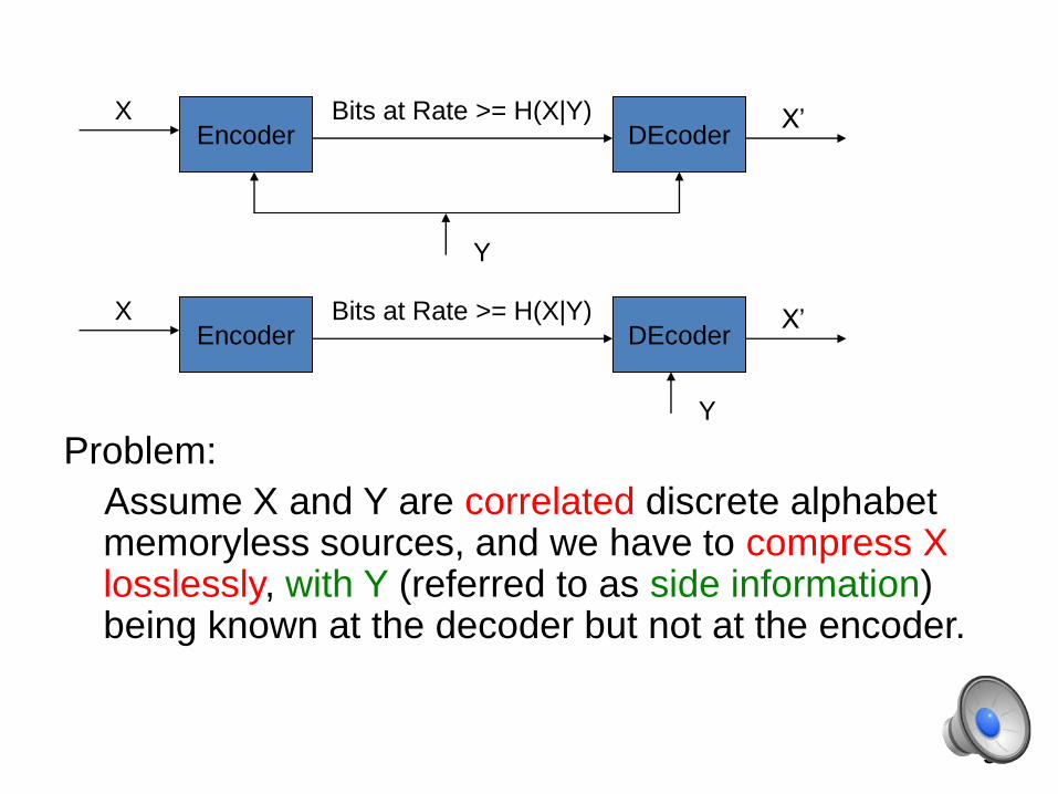
Problem:
Assume X and Y are correlated discrete alphabet memoryless sources, and we have to compress X losslessly, with Y (referred to as side information) being known at the decoder but not at the encoder.
3
Encoder DEcoderX Bits at Rate >= H(X|Y) X’
Y
Encoder DEcoderX Bits at Rate >= H(X|Y) X’
Y
If Y were known at both sides, then the
problem of compressing X is well-
understood : one can compress X at the
theoretical rate of its condition Entropy
given Y, H(X|Y).
But what if Y were known only at the
decoder for X and not at the encoder?
4
The answer is that one can still
compress X using only H(X|Y) bits, the
same as the case where the encoder
does know Y.
• By just knowing the joint distribution of X and Y,
without explicitly knowing Y, the encoder of X can
perform as well as an encoder which explicitly
knows Y.
• This is known as the Slepian-Wolf coding theorem.
5
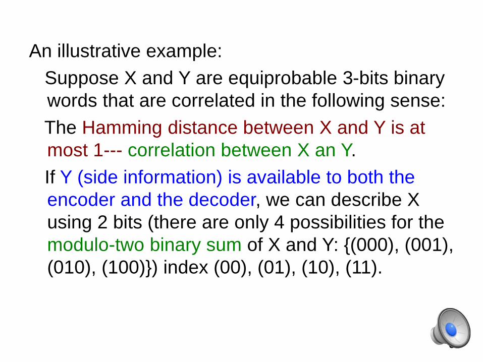
An illustrative example:
Suppose X and Y are equiprobable 3-bits binary
words that are correlated in the following sense:
The Hamming distance between X and Y is at
most 1--- correlation between X an Y.
If Y (side information) is available to both the
encoder and the decoder, we can describe X
using 2 bits (there are only 4 possibilities for the
modulo-two binary sum of X and Y: {(000), (001),
(010), (100)}) index (00), (01), (10), (11).
6
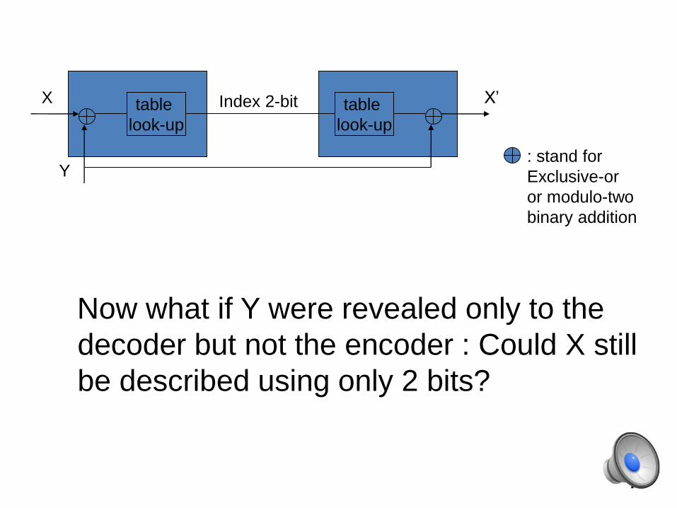
Now what if Y were revealed only to the
decoder but not the encoder : Could X still
be described using only 2 bits?
7
X
Y
table
look-up
Index 2-bit table
look-up
X’
: stand for
Exclusive-or
or modulo-two
binary addition
Since the decoder knows Y, it is wasteful for X to
spend any bits in differentiating between {X=(000)
and X=(111)}, since the Hamming distance between
these two codewords is 3 --- do not follow the
correlation constraint.
Thus, if the decoder knows that either X=(000) or
X=(111), it can resolve this uncertainly by checking
which of them is closer in Hamming distance to Y,
and declaring that as the value of X.
8
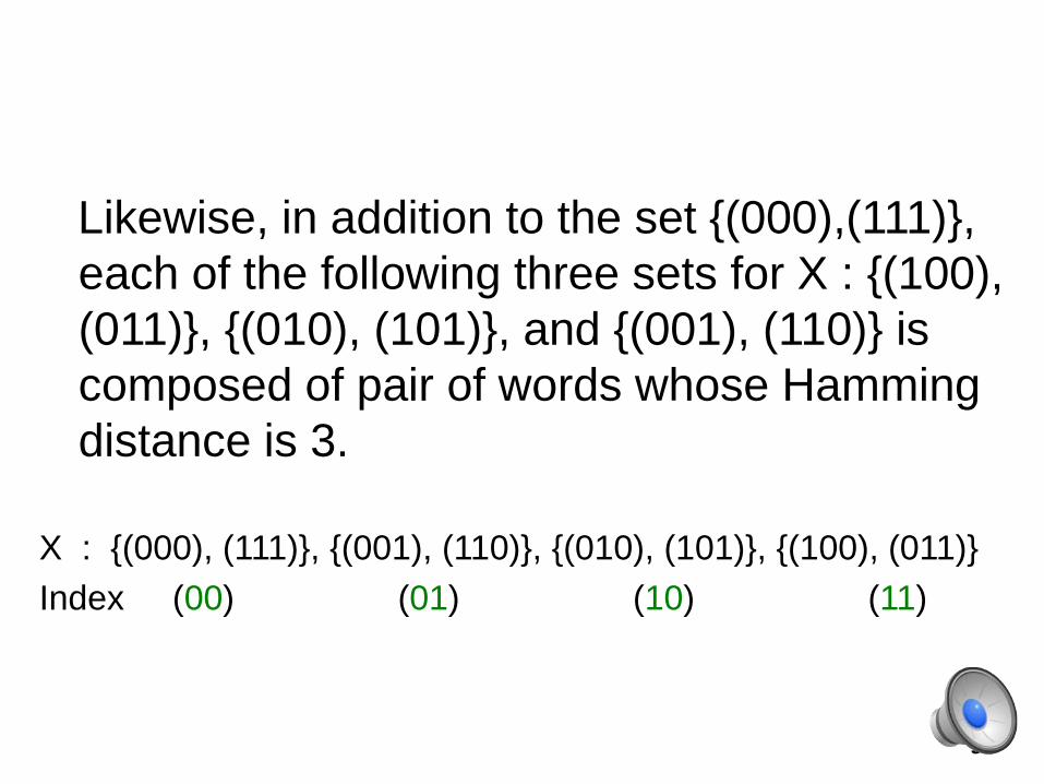
Likewise, in addition to the set {(000),(111)},
each of the following three sets for X : {(100),
(011)}, {(010), (101)}, and {(001), (110)} is
composed of pair of words whose Hamming
distance is 3.
X : {(000), (111)}, {(001), (110)}, {(010), (101)}, {(100), (011)}
Index (00) (01) (10) (11)
9
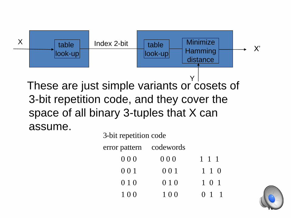
These are just simple variants or cosets of
3-bit repetition code, and they cover the
space of all binary 3-tuples that X can
assume.3-bit repetition code
error pattern codewords
0 0 0 0 0 0 1 1 1
0 0 1 0 0 1 1 1 0
0 1 0 0 1 0 1 0 1
1 0 0 1 0 0 0 1 1
10
X
Y
table
look-up
Index 2-bit table
look-upX’
Minimize
Hamming
distance
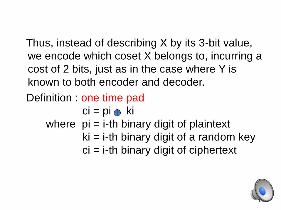
Thus, instead of describing X by its 3-bit value,
we encode which coset X belongs to, incurring a
cost of 2 bits, just as in the case where Y is
known to both encoder and decoder.
Definition : one time pad
ci = pi ki
where pi = i-th binary digit of plaintext
ki = i-th binary digit of a random key
ci = i-th binary digit of ciphertext
11
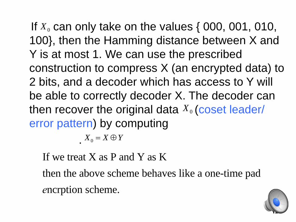
If can only take on the values { 000, 001, 010,
100}, then the Hamming distance between X and
Y is at most 1. We can use the prescribed
construction to compress X (an encrypted data) to
2 bits, and a decoder which has access to Y will
be able to correctly decoder X. The decoder can
then recover the original data (coset leader/
error pattern) by computing
.
0X
0X
12
YXX 0
If we treat X as P and Y as K
then the above scheme behaves like a one-time pad
encrption scheme.
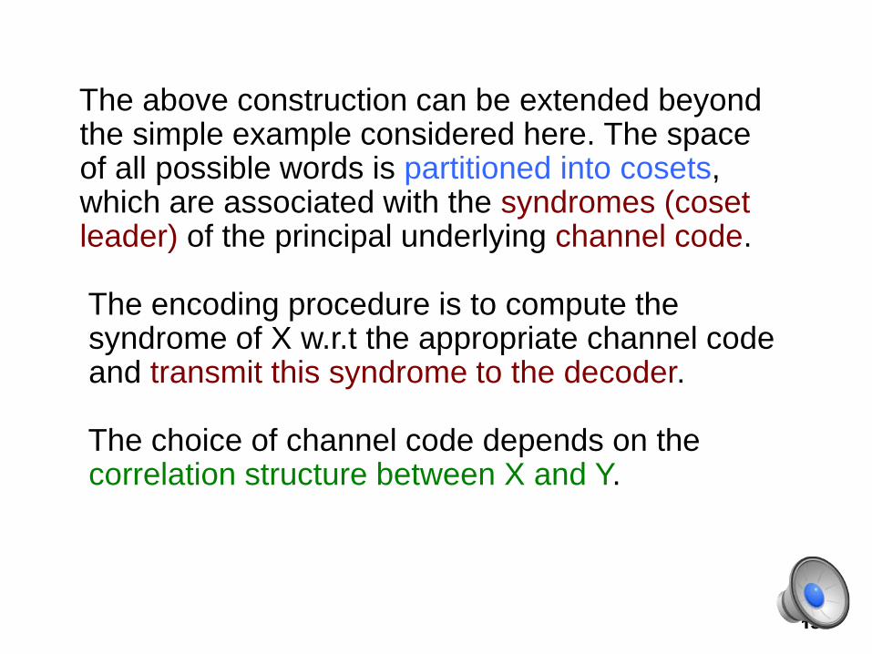
The above construction can be extended beyondthe simple example considered here. The space of all possible words is partitioned into cosets, which are associated with the syndromes (cosetleader) of the principal underlying channel code.
The encoding procedure is to compute the syndrome of X w.r.t the appropriate channel code and transmit this syndrome to the decoder.
The choice of channel code depends on the correlation structure between X and Y.
13
• If X and Y are more correlated, then the
required strength (length) of the code is
less (shorter).
• The decoding procedure is to identify the
closest codeword to Y in the coset
associated with the transmitted syndrome,
and declare that codeword to be X.
14
Encoding with a Fidelity Criterion
• A. Problem formulation
Here we consider the continuous-valued source X
and side-information Y. Specifically, X and Y are
correlated memoryless processes characterized
by independent and identically distributed (i.i.d)
sequences and ,respectively.
1}{ iiX
1}{ iiY
15
• We consider the special case where Y is a noise
version of X: i.e.,
is also continuous valued ( defined on the real
line ), i.i.d, and independent of the .
• As before, the decoder alone has access to the Y
process (side information), and the task is to
optimally compress the X process .
Yi = Xi +Ni,where{Ni}i=1
¥
16
sX i '
• For the rest of our discussion , we will confine
ourselves to the case where the and are
zero-mean Gaussian random variables with
known variances, so as to benchmark the
performance against the theoretical
performance bound.
sX i ' sNi '
17
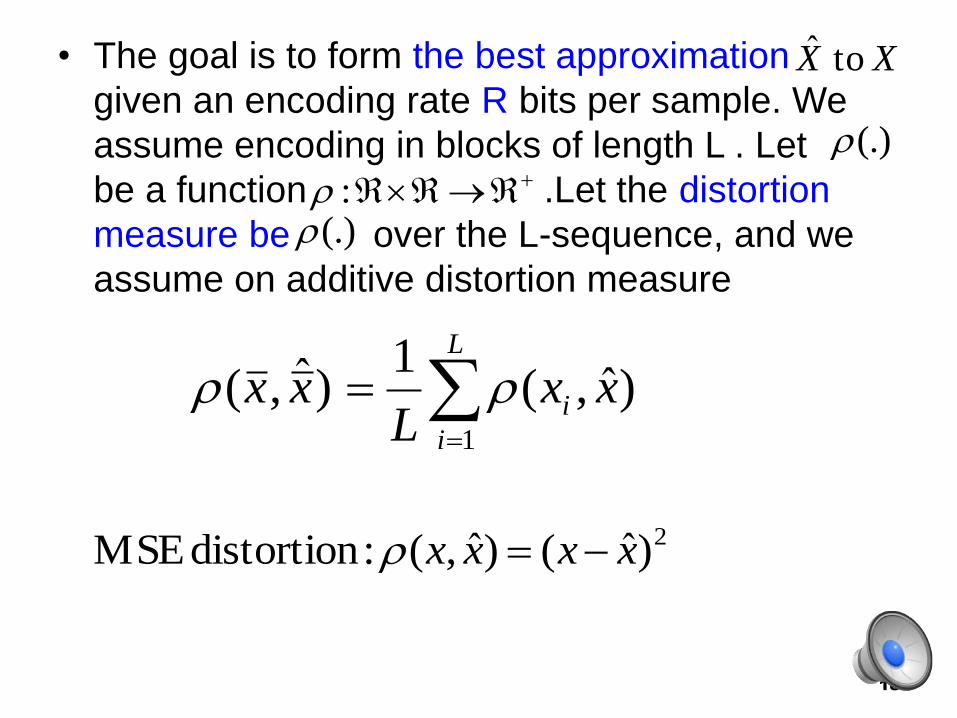
• The goal is to form the best approximation
given an encoding rate R bits per sample. We
assume encoding in blocks of length L . Let
be a function .Let the distortion
measure be over the L-sequence, and we
assume on additive distortion measure
XX toˆ
(.)
18
:
)ˆ,(1
)ˆ,(1
L
i
i xxL
xx
2)ˆ()ˆ,( :distortion MSE xxxx
(.)
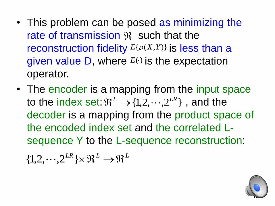
• This problem can be posed as minimizing the
rate of transmission such that the
reconstruction fidelity is less than a
given value D, where is the expectation
operator.
• The encoder is a mapping from the input space
to the index set: , and the
decoder is a mapping from the product space of
the encoded index set and the correlated L-
sequence Y to the L-sequence reconstruction:
)},({ YXE
19
)(E
}2,,2,1{ LRL
LLLR }2,,2,1{
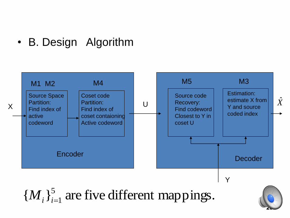
• B. Design Algorithm
mappings.different five are }{ 5
1iiM
X̂
20
Encoder
Source Space
Partition:
Find index of
active
codeword
Coset code
Partition:
Find index of
coset contaioning
Active codeword
X
M1 M2 M4 M5 M3
U
Source code
Recovery:
Find codeword
Closest to Y in
coset U
Estimation:
estimate X from
Y and source
coded index
Decoder
Y
mappings.different five are }{ 5
1iiM
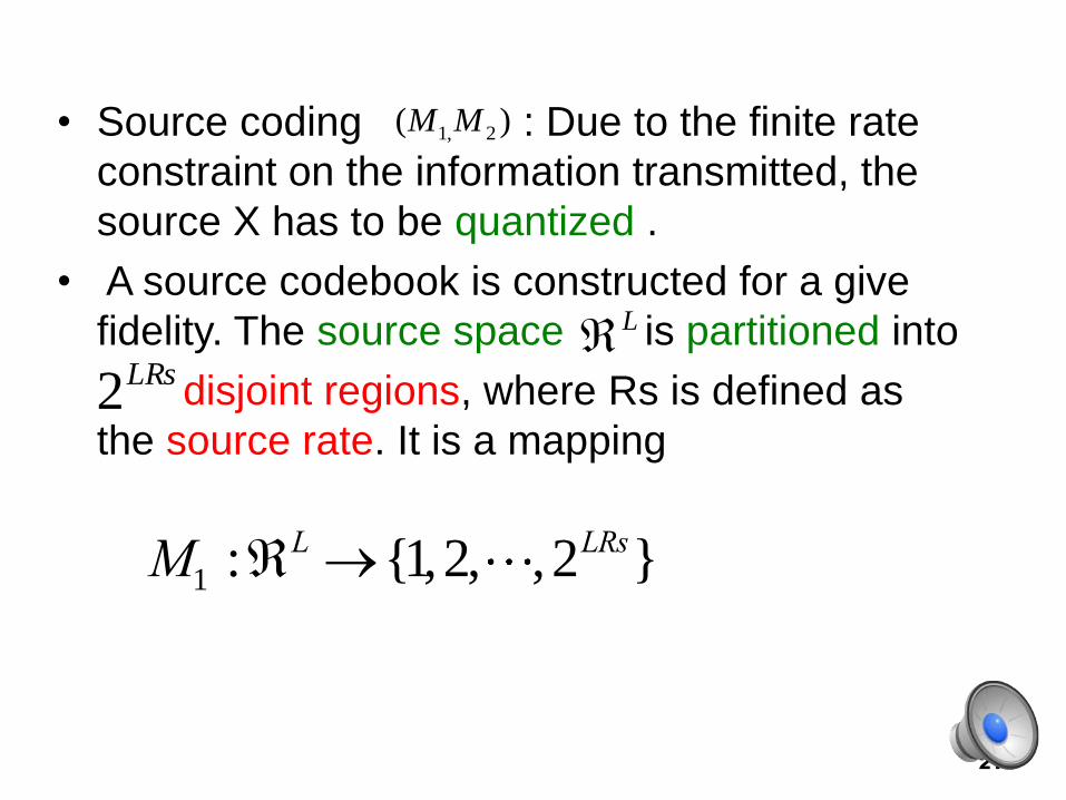
• Source coding : Due to the finite rate
constraint on the information transmitted, the
source X has to be quantized .
• A source codebook is constructed for a give
fidelity. The source space is partitioned into
disjoint regions, where Rs is defined as
the source rate. It is a mapping
)( 2,1 MM
M1 :ÂL®{1,2, ,2LRs}
21
LRs2
L
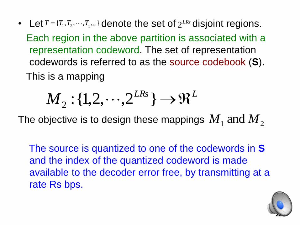
• Let denote the set of disjoint regions.
Each region in the above partition is associated with a
representation codeword. The set of representation
codewords is referred to as the source codebook (S).
This is a mapping
The objective is to design these mappings
The source is quantized to one of the codewords in S
and the index of the quantized codeword is made
available to the decoder error free, by transmitting at a
rate Rs bps.
},,,{221 LRsTTTT LRs2
22
LLRsM }2,,2,1{:2
21 and MM
• We refer to the representation codeword to which X is quantized as the active codeword. Let the random variable characterizing the active codeword be denoted by W. Note, unlike traditional source coding, the active codeword is not used as the reconstruction for the source (an extra ECC process will be involved).
• Rather, the decoding further involves “ estimationof the source” based on the available information about the source, the result of estimation is used as the final reconstruction.
23
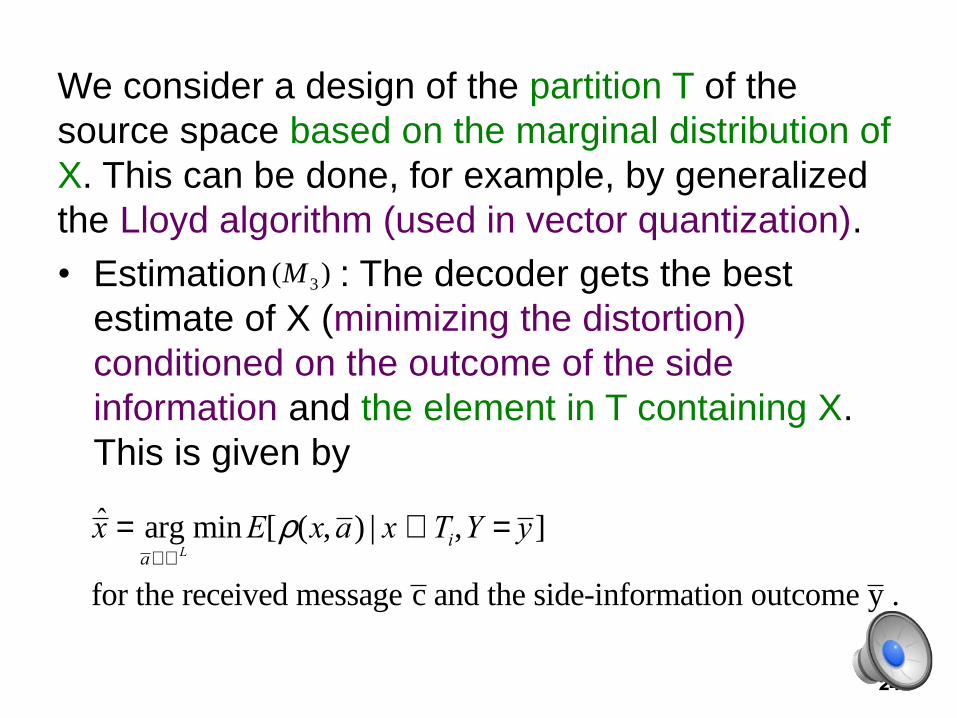
We consider a design of the partition T of the
source space based on the marginal distribution of
X. This can be done, for example, by generalized
the Lloyd algorithm (used in vector quantization).
• Estimation : The decoder gets the best
estimate of X (minimizing the distortion)
conditioned on the outcome of the side
information and the element in T containing X.
This is given by
)( 3M
x̂ = argaÎÂ
L
minE[r(x,a) | x Î Ti,Y = y]
for the received message c and the side-information outcome y .
24
• It can be interpreted as a mapping
The estimation error is a function of Rs, which is
chosen to keep this error within the given fidelity
criterion.
LLRsLM }2,,2,1{:3
25
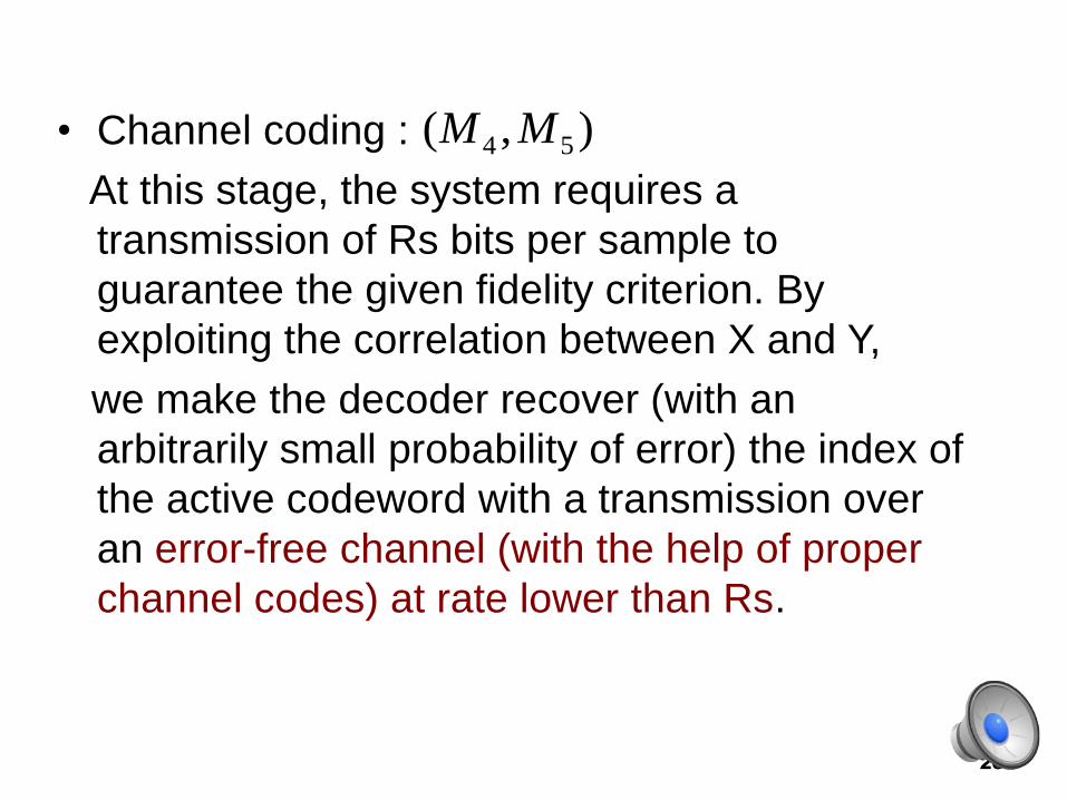
• Channel coding :
At this stage, the system requires a
transmission of Rs bits per sample to
guarantee the given fidelity criterion. By
exploiting the correlation between X and Y,
we make the decoder recover (with an
arbitrarily small probability of error) the index of
the active codeword with a transmission over
an error-free channel (with the help of proper
channel codes) at rate lower than Rs.
),( 54 MM
26
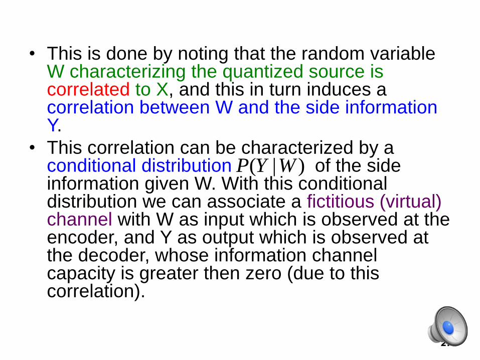
• This is done by noting that the random variable W characterizing the quantized source is correlated to X, and this in turn induces a correlation between W and the side information Y.
• This correlation can be characterized by a conditional distribution of the side information given W. With this conditional distribution we can associate a fictitious (virtual) channel with W as input which is observed at the encoder, and Y as output which is observed at the decoder, whose information channel capacity is greater then zero (due to this correlation).
)|( WYP
27
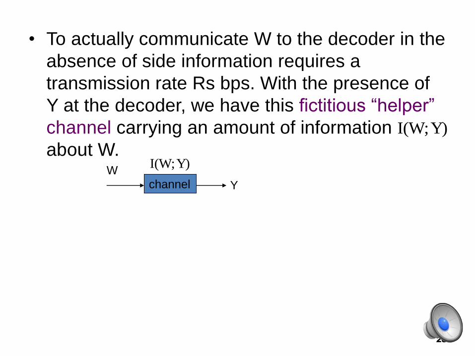
• To actually communicate W to the decoder in the
absence of side information requires a
transmission rate Rs bps. With the presence of
Y at the decoder, we have this fictitious “helper”
channel carrying an amount of information
about W.
Y)I(W;
Y)I(W;
28
channelW
Y
• The remaining uncertainly in W after observing
the side information Y is
H(W|Y) = H(W) – I(W;Y)
and this is the desired final rate of transmission.
The rebate(折扣) in the rate of transmission is
I(W;Y).
• Using this intuition, our goal is to get a rebate as
close to I(W;Y) as possible by building a
practical structured “channel code” (C’) for this
fictitions channel on the space of W.
29
• Let denote the number of codewords in the designed channel code where Rc is defined as the channel rate.
• Suppose for a given realization, the active codeword (say W) belongs to this channel code (such as Turbo-code, LDPC, LDPCA) and this is known at the decoder (say communicated by a genie), then we do not need to send any information to the receiver, as it can recover the intended codeword with a small probability of error by decoding Y with the aid of the channel code C’ . (this can be interpreted as transmitting W over the fictitions channel and observing the output of this channel Y as side information at the decoder).
LRc2
30
• Since, in general, any codeword in the source codebook can be a quantization outcome with a nonzero probability, we partition the source codebook space into cosets of this channel code. The channel code is designed in such a way that “Each of Its Cosets is also an Equally Good Channel code for the channel P(Y|W)”.
• Thus, each quantization outcome belongs to a coset of this channel code, and this along has to be converged to the decoder, which can then proceed to use this coset of channel code for finding the intended active codeword.
31
• The encoder computes the index of the coset of
the channel code containing the active
codeword using a mapping
and transmit this information with rate
bits per sample to the decoder.
M4 :{1,2, ,2LRs}®{1,2, ,2LRc}
cs RRR
32
• The decoder recovers the active codeword in
the signaled coset by finding (channel coding)
the most likely codeword given the observed
side information. This is characterized by a
mapping
}2,,2,1{}2,,2,1{:5sLRLRLM
33
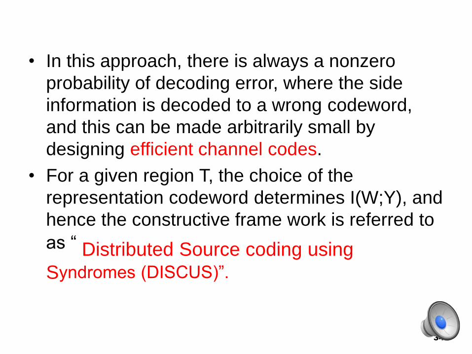
• In this approach, there is always a nonzero
probability of decoding error, where the side
information is decoded to a wrong codeword,
and this can be made arbitrarily small by
designing efficient channel codes.
• For a given region T, the choice of the
representation codeword determines I(W;Y), and
hence the constructive frame work is referred to
as “ Distributed Source coding using
Syndromes (DISCUS)”.
34
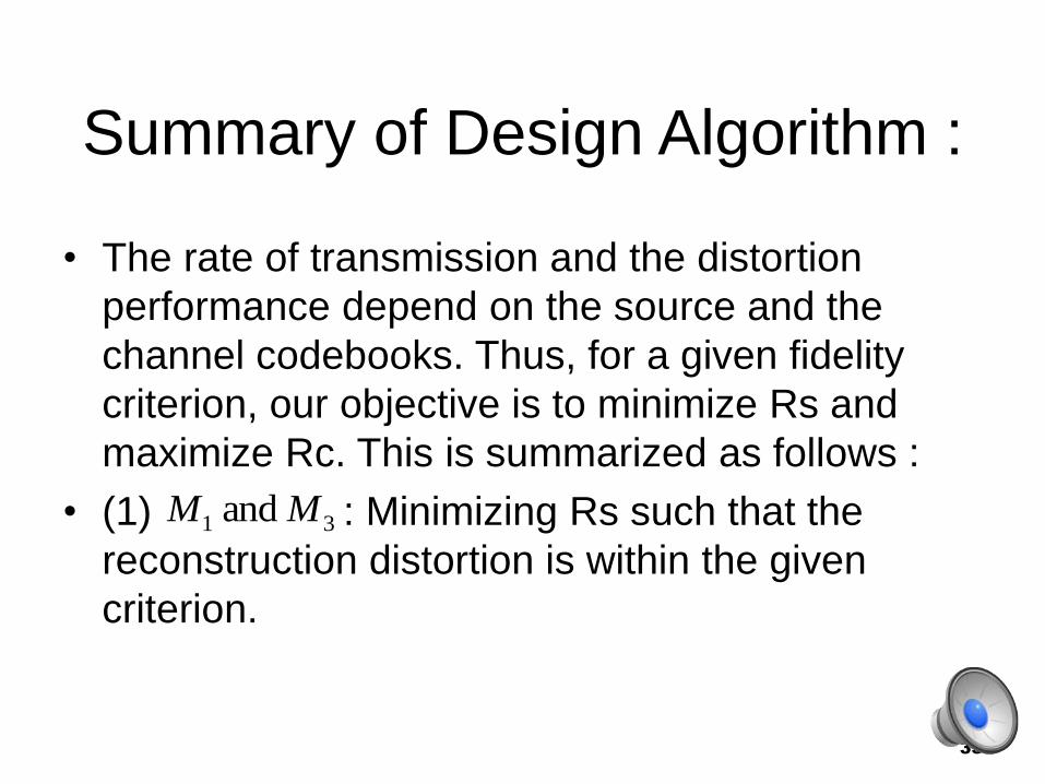
Summary of Design Algorithm :
• The rate of transmission and the distortion
performance depend on the source and the
channel codebooks. Thus, for a given fidelity
criterion, our objective is to minimize Rs and
maximize Rc. This is summarized as follows :
• (1) : Minimizing Rs such that the
reconstruction distortion is within the given
criterion.
31 and MM
35
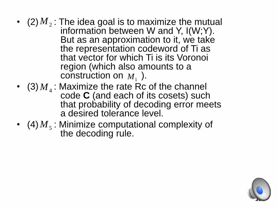
• (2) : The idea goal is to maximize the mutual information between W and Y, I(W;Y). But as an approximation to it, we take the representation codeword of Ti as that vector for which Ti is its Voronoi region (which also amounts to a construction on ).
• (3) : Maximize the rate Rc of the channel code C (and each of its cosets) such that probability of decoding error meets a desired tolerance level.
• (4) : Minimize computational complexity of the decoding rule.
1M
2M
36
4M
5M
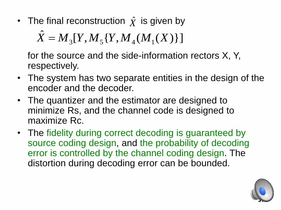
• The final reconstruction is given by
for the source and the side-information rectors X, Y, respectively.
• The system has two separate entities in the design of the encoder and the decoder.
• The quantizer and the estimator are designed to minimize Rs, and the channel code is designed to maximize Rc.
• The fidelity during correct decoding is guaranteed by source coding design, and the probability of decoding error is controlled by the channel coding design. The distortion during decoding error can be bounded.
X̂
)}]((,{,[ˆ1453 XMMYMYMX
37
A Video Coding Architecture
Based on Distributed
compression Principles
38
• In the near future, multiple video input and
output streams are expected to be used to
enhance user experience. These streams
need to be captured using a network of
distributed devices and transmitted over a
bandwidth constrained, noisy wireless
transmission medium, to a central location
for processing, with the goal for example,
of creating high-resolution video using
inexpensive cameras.
39
Uplink rich media application
V.S.
Downlink video delivery model (traditional approach)
New demands:
• low-power and light-footprint encoding due to limited power and/or device memory.
• high compression efficiency due to both bandwidth and transmission power limitation.
• robustness to packet/frame loss caused by channel transmission errors.
40
H.26x/MPEG and HEVC video coding
standards:
Computationally heavy at the encoder
(primarily due to motion-search) and very
fragile to packet loss
they achieve state-of-the-art
compression efficiency but fail to meet
the other two criteria.
41
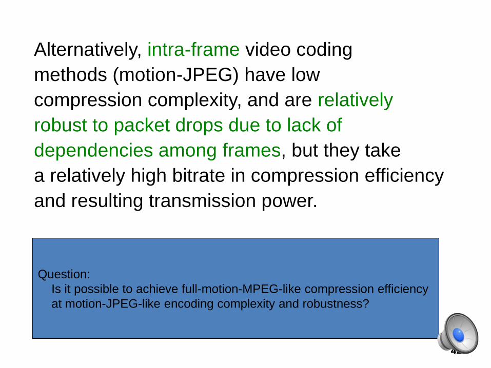
Alternatively, intra-frame video coding
methods (motion-JPEG) have low
compression complexity, and are relatively
robust to packet drops due to lack of
dependencies among frames, but they take
a relatively high bitrate in compression efficiency
and resulting transmission power.
42
Question:
Is it possible to achieve full-motion-MPEG-like compression efficiency
at motion-JPEG-like encoding complexity and robustness?
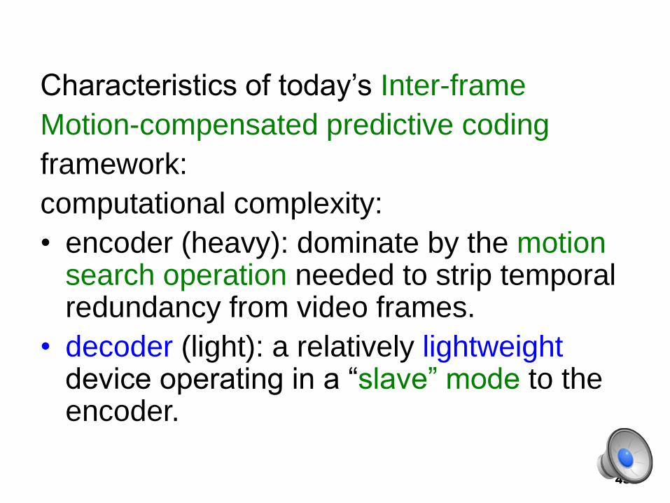
Characteristics of today’s Inter-frame
Motion-compensated predictive coding
framework:
computational complexity:
• encoder (heavy): dominate by the motion search operation needed to strip temporal redundancy from video frames.
• decoder (light): a relatively lightweight device operating in a “slave” mode to the encoder.
43
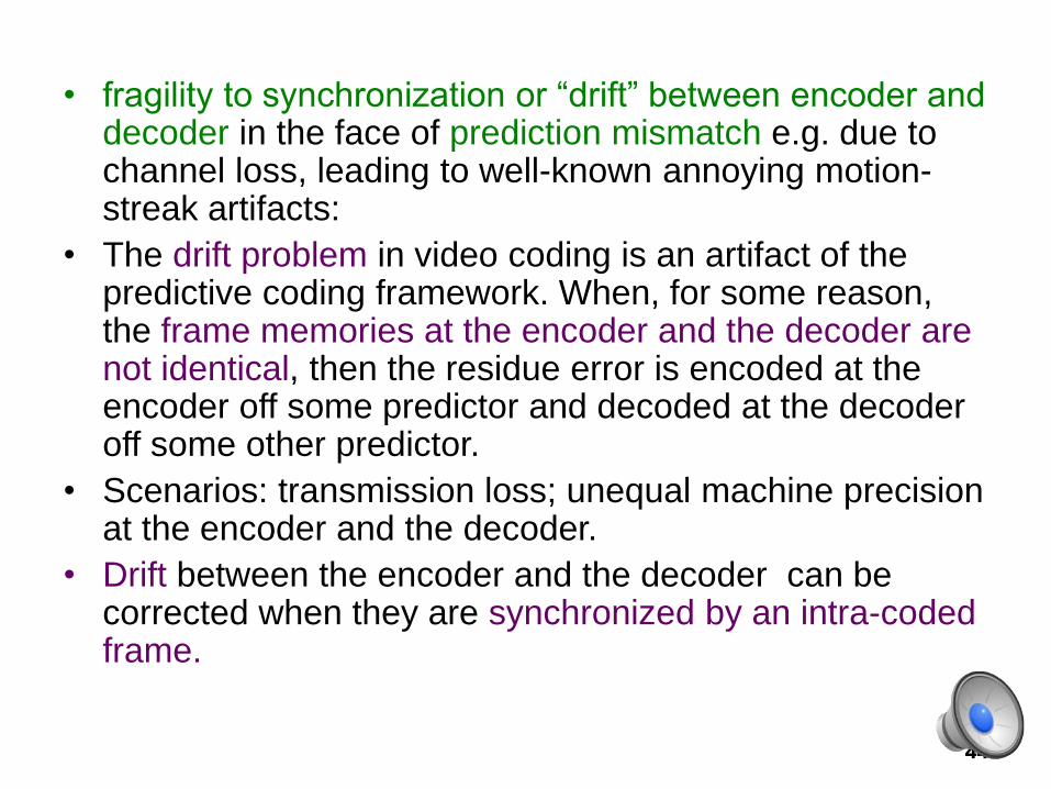
• fragility to synchronization or “drift” between encoder and decoder in the face of prediction mismatch e.g. due to channel loss, leading to well-known annoying motion-streak artifacts:
• The drift problem in video coding is an artifact of the predictive coding framework. When, for some reason, the frame memories at the encoder and the decoder are not identical, then the residue error is encoded at the encoder off some predictor and decoded at the decoder off some other predictor.
• Scenarios: transmission loss; unequal machine precision at the encoder and the decoder.
• Drift between the encoder and the decoder can be corrected when they are synchronized by an intra-coded frame.
44
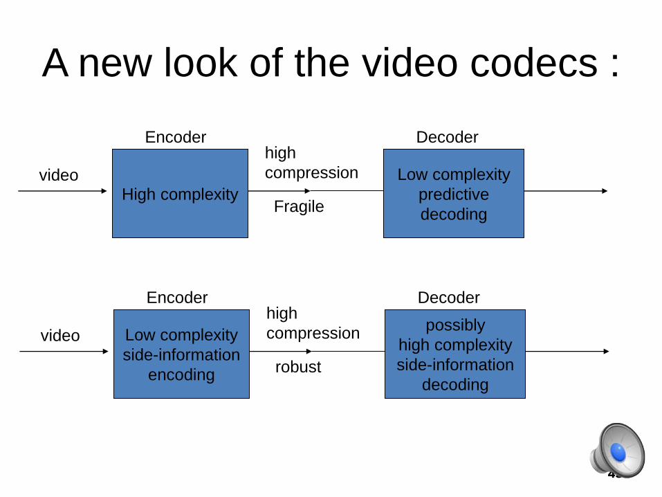
A new look of the video codecs :
45
High complexity
Low complexity
predictive
decoding
video
high
compression
Fragile
DecoderEncoder
Low complexity
side-information
encoding
possibly
high complexity
side-information
decoding
video
high
compression
robust
DecoderEncoder
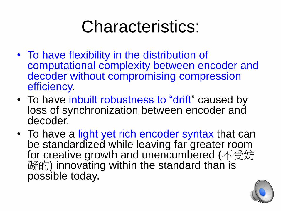
Characteristics:
• To have flexibility in the distribution of computational complexity between encoder and decoder without compromising compression efficiency.
• To have inbuilt robustness to “drift” caused by loss of synchronization between encoder and decoder.
• To have a light yet rich encoder syntax that can be standardized while leaving far greater room for creative growth and unencumbered (不受妨礙的) innovating within the standard than is possible today.
46
The investigation of new video codec
discussed in the following is found on the
principles of
• Distributed Source Coding (DSC)
• Channel coding
• Video Transcoding (DSC-to-HEVC)
47
• In uplink-rich multimedia application, it is
desirable to share the complexity burden
between encoder and decoder more equally or
in any desirable ratio as demanded by a specific
application scenario.
• Target : a maximally thin encoder
moving the expensive motion estimation
component of the video codec from the encoder
to the decoder without loss of compression
efficiency in theory and with acceptable loss of
efficiency in practice.
48
• For robustness, we have to dispense with
the predictive frame work and change it by
a universally robust side-information
based coding framework.
• Side-information source coding inherently
consists of “good” channel codes, and
therefore, has naturally inbuilt robustness
to the synchronization loss issues.
49
• Traditional multimedia coding standards constrain the bit-stream syntax at the encoder=> There is relatively little room for creativity within the standard.
• If all the sophisticated signal processing task are performed at the decoder, the syntax of the encoder becomes rich enough to accommodate a variety of decoders that are all “Syntax-compatible”. => this opens up the opportunity of a whole new set of creative algorithms/techniques for motion-estimation, postprocessing and other critical signal processing tasks.
50
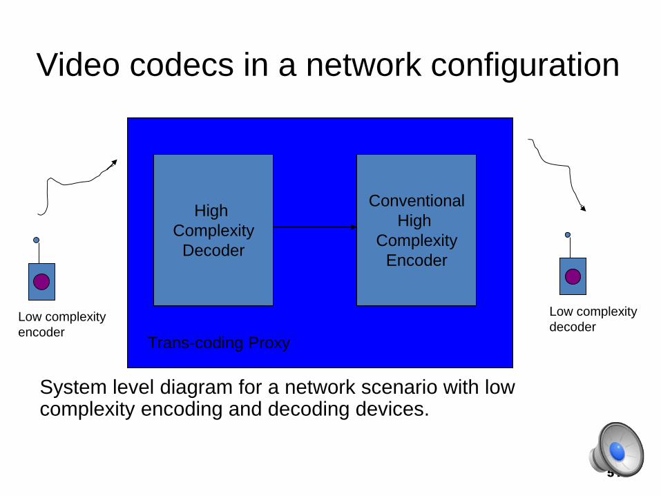
Video codecs in a network configuration
System level diagram for a network scenario with low complexity encoding and decoding devices.
51
Trans-coding Proxy
High
Complexity
Decoder
Conventional
High
Complexity
Encoder
Low complexity
encoder
Low complexity
decoder
• Under this architecture, the entire
computational burden has been absorbed
into the network device (such as Base
Station or Cloud). Both the end devices,
which are battery-constrained, run power
efficient and light encoding and decoding
algorithms. =
Match the developing trend of
Mobile-First !
52
Summary
• Under the introduced construction, the relation used to decompose the source ( such as inter-frame-relationship) behaves like the correlation between the source, while the subsets or associated representation codewords ( noisy versions of estimated input) behave like the side-information Y.
53
• The number of syndromes determines the bandwidth between the encoder and decoder and therefore determines the data reduction ( or compression ratio) of the system.
• Since the mapping between the subsets and ECC can be done in an encryption manner, therefore, one can compress an encrypted data.
54


![IJCST Vo l . 6, ISS ue 4, oCT - D 2015 Enhanced Hiding ... · PDF fileIterative Reconstruction for Encrypted Image [6] describes novel scheme for lossy compression of an encrypted](https://img.pdfslide.us/doc/110x75/5abe2d4f7f8b9a8e3f8cad7b/ijcst-vo-l-6-iss-ue-4-oct-d-2015-enhanced-hiding-reconstruction-for-encrypted.jpg)