On Clustering Validation Techniques · 108 HALKIDI, BATISTAKIS AND VAZIRGIANNIS Figure 1.Steps of clustering process. The clustering process may result in different partitioning of

Journal of Intelligent Information Systems, 17:2/3, 107–145, 2001c© 2001 Kluwer Academic Publishers. Manufactured in The Netherlands.

On Clustering Validation Techniques

MARIA HALKIDI [email protected] BATISTAKIS [email protected] VAZIRGIANNIS [email protected] of Informatics, Athens University of Economics & Business, Patision 76, 10434, Athens,Greece (Hellas)

Abstract. Cluster analysis aims at identifying groups of similar objects and, therefore helps to discover dis-tribution of patterns and interesting correlations in large data sets. It has been subject of wide research since itarises in many application domains in engineering, business and social sciences. Especially, in the last years theavailability of huge transactional and experimental data sets and the arising requirements for data mining createdneeds for clustering algorithms that scale and can be applied in diverse domains.

This paper introduces the fundamental concepts of clustering while it surveys the widely known clustering algo-rithms in a comparative way. Moreover, it addresses an important issue of clustering process regarding the qualityassessment of the clustering results. This is also related to the inherent features of the data set under concern. A re-view of clustering validity measures and approaches available in the literature is presented. Furthermore, the paperillustrates the issues that are under-addressed by the recent algorithms and gives the trends in clustering process.

Keywords: clustering algorithms, unsupervised learning, cluster validity, validity indices

1. Introduction

Clustering is one of the most useful tasks in data mining process for discovering groups andidentifying interesting distributions and patterns in the underlying data. Clustering problemis about partitioning a given data set into groups (clusters) such that the data points in acluster are more similar to each other than points in different clusters (Guha et al., 1998).For example, consider a retail database records containing items purchased by customers.A clustering procedure could group the customers in such a way that customers with similarbuying patterns are in the same cluster. Thus, the main concern in the clustering processis to reveal the organization of patterns into “sensible” groups, which allow us to discoversimilarities and differences, as well as to derive useful conclusions about them. This idea isapplicable in many fields, such as life sciences, medical sciences and engineering. Clusteringmay be found under different names in different contexts, such as unsupervised learning(in pattern recognition), numerical taxonomy (in biology, ecology), typology (in socialsciences) and partition (in graph theory) (Theodoridis and Koutroubas, 1999).

In the clustering process, there are no predefined classes and no examples that would showwhat kind of desirable relations should be valid among the data that is why it is perceivedas an unsupervised process (Berry and Linoff, 1996). On the other hand, classification is aprocedure of assigning a data item to a predefined set of categories (Fayyad et al., 1996).Clustering produces initial categories in which values of a data set are classified during theclassification process.

108 HALKIDI, BATISTAKIS AND VAZIRGIANNIS

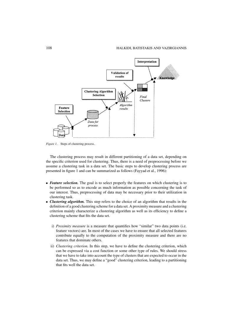
Figure 1. Steps of clustering process.

The clustering process may result in different partitioning of a data set, depending onthe specific criterion used for clustering. Thus, there is a need of preprocessing before weassume a clustering task in a data set. The basic steps to develop clustering process arepresented in figure 1 and can be summarized as follows (Fayyad et al., 1996):

• Feature selection. The goal is to select properly the features on which clustering is tobe performed so as to encode as much information as possible concerning the task ofour interest. Thus, preprocessing of data may be necessary prior to their utilization inclustering task.

• Clustering algorithm. This step refers to the choice of an algorithm that results in thedefinition of a good clustering scheme for a data set. A proximity measure and a clusteringcriterion mainly characterize a clustering algorithm as well as its efficiency to define aclustering scheme that fits the data set.

i) Proximity measure is a measure that quantifies how “similar” two data points (i.e.feature vectors) are. In most of the cases we have to ensure that all selected featurescontribute equally to the computation of the proximity measure and there are nofeatures that dominate others.

ii) Clustering criterion. In this step, we have to define the clustering criterion, whichcan be expressed via a cost function or some other type of rules. We should stressthat we have to take into account the type of clusters that are expected to occur in thedata set. Thus, we may define a “good” clustering criterion, leading to a partitioningthat fits well the data set.

CLUSTERING VALIDATION TECHNIQUES 109

• Validation of the results. The correctness of clustering algorithm results is verified usingappropriate criteria and techniques. Since clustering algorithms define clusters that arenot known a priori, irrespective of the clustering methods, the final partition of datarequires some kind of evaluation in most applications (Rezaee et al., 1998).

• Interpretation of the results. In many cases, the experts in the application area have tointegrate the clustering results with other experimental evidence and analysis in order todraw the right conclusion.

1.1. Clustering applications

Cluster analysis is a major tool in a number of applications in many fields of business andscience. Hereby, we summarize the basic directions in which clustering is used (Theodoridisand Koutroubas, 1999):

• Data reduction. Cluster analysis can contribute in compression of the information in-cluded in data. In several cases, the amount of available data is very large and its pro-cessing becomes very demanding. Clustering can be used to partition data set into anumber of “interesting” clusters. Then, instead of processing the data set as an entity, weadopt the representatives of the defined clusters in our process. Thus, data compression isachieved.

• Hypothesis generation. Cluster analysis is used here in order to infer some hypothesesconcerning the data. For instance we may find in a retail database that there are twosignificant groups of customers based on their age and the time of purchases. Then,we may infer some hypotheses for the data, that it, “young people go shopping in theevening”, “old people go shopping in the morning”.

• Hypothesis testing. In this case, the cluster analysis is used for the verification of thevalidity of a specific hypothesis. For example, we consider the following hypothesis:“Young people go shopping in the evening”. One way to verify whether this is true isto apply cluster analysis to a representative set of stores. Suppose that each store isrepresented by its customer’s details (age, job etc) and the time of transactions. If, afterapplying cluster analysis, a cluster that corresponds to “young people buy in the evening”is formed, then the hypothesis is supported by cluster analysis.

• Prediction based on groups. Cluster analysis is applied to the data set and the resultingclusters are characterized by the features of the patterns that belong to these clusters.Then, unknown patterns can be classified into specified clusters based on their simi-larity to the clusters’ features. Useful knowledge related to our data can be extracted.Assume, for example, that the cluster analysis is applied to a data set concerning patientsinfected by the same disease. The result is a number of clusters of patients, accordingto their reaction to specific drugs. Then for a new patient, we identify the cluster inwhich he/she can be classified and based on this decision his/her medication can bemade.

More specifically, some typical applications of the clustering are in the following fields(Han and Kamber, 2001):


• Business. In business, clustering may help marketers discover significant groups in theircustomers’ database and characterize them based on purchasing patterns.

• Biology. In biology, it can be used to define taxonomies, categorize genes with similarfunctionality and gain insights into structures inherent in populations.

• Spatial data analysis. Due to the huge amounts of spatial data that may be obtained fromsatellite images, medical equipment, Geographical Information Systems (GIS), imagedatabase exploration etc., it is expensive and difficult for the users to examine spatial datain detail. Clustering may help to automate the process of analysing and understandingspatial data. It is used to identify and extract interesting characteristics and patterns thatmay exist in large spatial databases.

• Web mining. In this case, clustering is used to discover significant groups of documentson the Web huge collection of semi-structured documents. This classification of Webdocuments assists in information discovery.

In general terms, clustering may serve as a pre-processing step for other algorithms, suchas classification, which would then operate on the detected clusters.

1.2. Clustering algorithms categories

A multitude of clustering methods are proposed in the literature. Clustering algorithms canbe classified according to:

• The type of data input to the algorithm.• The clustering criterion defining the similarity between data points.• The theory and fundamental concepts on which clustering analysis techniques are based

(e.g. fuzzy theory, statistics).

Thus according to the method adopted to define clusters, the algorithms can be broadlyclassified into the following types (Jain et al., 1999):

• Partitional clustering attempts to directly decompose the data set into a set of disjointclusters. More specifically, they attempt to determine an integer number of partitions thatoptimise a certain criterion function. The criterion function may emphasize the local orglobal structure of the data and its optimization is an iterative procedure.

• Hierarchical clustering proceeds successively by either merging smaller clusters intolarger ones, or by splitting larger clusters. The result of the algorithm is a tree of clusters,called dendrogram, which shows how the clusters are related. By cutting the dendrogramat a desired level, a clustering of the data items into disjoint groups is obtained.

• Density-based clustering. The key idea of this type of clustering is to group neighbouringobjects of a data set into clusters based on density conditions.

• Grid-based clustering. This type of algorithms is mainly proposed for spatial data mining.Their main characteristic is that they quantise the space into a finite number of cells andthen they do all operations on the quantised space.


For each of above categories there is a wealth of subtypes and different algorithms forfinding the clusters. Thus, according to the type of variables allowed in the data set can becategorized into (Guha et al., 1999; Huang et al., 1997; Rezaee et al., 1998):

• Statistical, which are based on statistical analysis concepts. They use similarity measuresto partition objects and they are limited to numeric data.

• Conceptual, which are used to cluster categorical data. They cluster objects according tothe concepts they carry.

Another classification criterion is the way clustering handles uncertainty in terms ofcluster overlapping.

• Fuzzy clustering, which uses fuzzy techniques to cluster data and they consider thatan object can be classified to more than one clusters. This type of algorithms leads toclustering schemes that are compatible with everyday life experience as they handle theuncertainty of real data. The most important fuzzy clustering algorithm is Fuzzy C-Means(Bezdeck et al., 1984).

• Crisp clustering, considers non-overlapping partitions meaning that a data point eitherbelongs to a class or not. Most of the clustering algorithms result in crisp clusters, andthus can be categorized in crisp clustering.

• Kohonen net clustering, which is based on the concepts of neural networks. The Kohonennetwork has input and output nodes. The input layer (input nodes) has a node for eachattribute of the record, each one connected to every output node (output layer). Eachconnection is associated with a weight, which determines the position of the correspond-ing output node. Thus, according to an algorithm, which changes the weights properly,output nodes move to form clusters.

In general terms, the clustering algorithms are based on a criterion for assessing thequality of a given partitioning. More specifically, they take as input some parameters (e.g.number of clusters, density of clusters) and attempt to define the best partitioning of a dataset for the given parameters. Thus, they define a partitioning of a data set based on certainassumptions and not necessarily the “best” one that fits the data set.

Since clustering algorithms discover clusters, which are not known a priori, the finalpartitions of a data set requires some sort of evaluation in most applications (Rezaee et al.,1998). For instance questions like “how many clusters are there in the data set?”, “does theresulting clustering scheme fits our data set?”, “is there a better partitioning for our dataset?” call for clustering results validation and are the subjects of methods discussed in theliterature. They aim at the quantitative evaluation of the results of the clustering algorithmsand are known under the general term cluster validity methods.

The remainder of the paper is organized as follows. In the next section we present themain categories of clustering algorithms that are available in literature. Then, in Section 3we discuss the main characteristics of these algorithms in a comparative way. In Section 4we present the main concepts of clustering validity indices and the techniques proposed inliterature for evaluating the clustering results. Moreover, an experimental study based onsome of these validity indices is presented in Section 5, using synthetic and real data sets.We conclude in Section 6 by summarizing and providing the trends in clustering.


2. Clustering algorithms

In recent years, a number of clustering algorithms has been proposed and is available in theliterature. Some representative algorithms of the above categories follow.

2.1. Partitional algorithms

In this category, K-Means is a commonly used algorithm (MacQueen, 1967). The aim ofK-Means clustering is the optimisation of an objective function that is described by theequation

E =c∑

i=1

∑x∈Ci

d(x, mi ) (1)

In the above equation, mi is the center of cluster Ci , while d(x, mi ) is the Euclideandistance between a point x and mi . Thus, the criterion function Eattempts to minimizethe distance of each point from the center of the cluster to which the point belongs.More specifically, the algorithm begins by initialising a set of c cluster centers. Then,it assigns each object of the dataset to the cluster whose center is the nearest, and re-computes the centers. The process continues until the centers of the clusters stopchanging.

Another algorithm of this category is PAM (Partitioning Around Medoids). The objectiveof PAM is to determine a representative object (medoid) for each cluster, that is, to findthe most centrally located objects within the clusters. The algorithm begins by selecting anobject as medoid for each of c clusters. Then, each of the non-selected objects is groupedwith the medoid to which it is the most similar. PAM swaps medoids with other non-selectedobjects until all objects qualify as medoid. It is clear that PAM is an expensive algorithmas regards finding the medoids, as it compares an object with entire dataset (Ng and Han,1994).

CLARA (Clustering Large Applications), is an implementation of PAM in a subset of thedataset. It draws multiple samples of the dataset, applies PAM on samples, and then outputsthe best clustering out of these samples (Ng and Han, 1994).

CLARANS (Clustering Large Applications based on Randomized Search), combines thesampling techniques with PAM. The clustering process can be presented as searching a graphwhere every node is a potential solution, that is, a set of k medoids. The clustering obtainedafter replacing a medoid is called the neighbour of the current clustering. CLARANS selectsa node and compares it to a user-defined number of their neighbours searching for a localminimum. If a better neighbour is found (i.e., having lower-square error), CLARANS movesto the neighbour’s node and the process start again; otherwise the current clustering is a localoptimum. If the local optimum is found, CLARANS starts with a new randomly selectednode in search for a new local optimum.

Finally K -prototypes, K-mode (Huang, 1997) are based on K -Means algorithm, but theyaim at clustering categorical data.


2.2. Hierarchical algorithms

Hierarchical clustering algorithms according to the method that produce clusters can furtherbe divided into (Theodoridis and Koutroubas, 1999):

• Agglomerative algorithms. They produce a sequence of clustering schemes of decreasingnumber of clusters at east step. The clustering scheme produced at each step results fromthe previous one by merging the two closest clusters into one.

• Divisive algorithms. These algorithms produce a sequence of clustering schemes of in-creasing number of clusters at each step. Contrary to the agglomerative algorithms theclustering produced at each step results from the previous one by splitting a cluster intotwo.

In sequel, we describe some representative hierarchical clustering algorithms.BIRCH (Zhang et al., 1996) uses a hierarchical data structure called CF-tree for parti-

tioning the incoming data points in an incremental and dynamic way. CF-tree is a height-balanced tree, which stores the clustering features and it is based on two parameters:branching factor B and threshold T, which referred to the diameter of a cluster (the di-ameter (or radius) of each cluster must be less than T ). BIRCH can typically find a goodclustering with a single scan of the data and improve the quality further with a few additionalscans. It is also the first clustering algorithm to handle noise effectively (Zhang et al., 1996).However, it does not always correspond to a natural cluster, since each node in CF-tree canhold a limited number of entries due to its size. Moreover, it is order-sensitive as it maygenerate different clusters for different orders of the same input data.

CURE (Guha et al., 1998) represents each cluster by a certain number of points that aregenerated by selecting well-scattered points and then shrinking them toward the clustercentroid by a specified fraction. It uses a combination of random sampling and partitionclustering to handle large databases.

ROCK (Guha et al., 1999), is a robust clustering algorithm for Boolean and categoricaldata. It introduces two new concepts, that is a point’s neighbours and links, and it is basedon them in order to measure the similarity/proximity between a pair of data points.

2.3. Density-based algorithms

Density based algorithms typically regard clusters as dense regions of objects in the dataspace that are separated by regions of low density.

A widely known algorithm of this category is DBSCAN (Ester et al., 1996). The key idea inDBSCAN is that for each point in a cluster, the neighbourhood of a given radius has to containat least a minimum number of points. DBSCAN can handle noise (outliers) and discoverclusters of arbitrary shape. Moreover, DBSCAN is used as the basis for an incrementalclustering algorithm proposed in Ester et al. (1998). Due to its density-based nature, theinsertion or deletion of an object affects the current clustering only in the neighbourhoodof this object and thus efficient algorithms based on DBSCAN can be given for incrementalinsertions and deletions to an existing clustering (Ester et al., 1998).

In Hinneburg and Keim (1998) another density-based clustering algorithm, DENCLUE, isproposed. This algorithm introduces a new approach to cluster large multimedia databases.


The basic idea of this approach is to model the overall point density analytically as the sumof influence functions of the data points. The influence function can be seen as a function,which describes the impact of a data point within its neighbourhood. Then clusters can beidentified by determining density attractors. Density attractors are local maximum of theoverall density function. In addition, clusters of arbitrary shape can be easily described by asimple equation based on overall density function. The main advantages of DENCLUE arethat it has good clustering properties in data sets with large amounts of noise and it allows acompact mathematically description of arbitrary shaped clusters in high-dimensional datasets. However, DENCLUE clustering is based on two parameters and as in most otherapproaches the quality of the resulting clustering depends on the choice of them. Theseparameters are (Hinneburg and Keim, 1998): i) parameter N which determines the influenceof a data point in its neighbourhood and ii) < describes whether a density-attractor issignificant, allowing a reduction of the number of density-attractors and helping to improvethe performance.

2.4. Grid-based algorithms

Recently a number of clustering algorithms have been presented for spatial data, known asgrid-based algorithms. These algorithms quantise the space into a finite number of cells andthen do all operations on the quantised space.

STING (Statistical Information Grid-based method) is representative of this category. Itdivides the spatial area into rectangular cells using a hierarchical structure. STING (Wanget al., 1997) goes through the data set and computes the statistical parameters (such asmean, variance, minimum, maximum and type of distribution) of each numerical featureof the objects within cells. Then it generates a hierarchical structure of the grid cells so asto represent the clustering information at different levels. Based on this structure STINGenables the usage of clustering information to search for queries or the efficient assignmentof a new object to the clusters.

WaveCluster (Sheikholeslami et al., 1998) is the latest grid-based algorithm proposed inliterature. It is based on signal processing techniques (wavelet transformation) to convertthe spatial data into frequency domain. More specifically, it first summarizes the data byimposing a multidimensional grid structure onto the data space (Han and Kamber, 2001).Each grid cell summarizes the information of a group of points that map into the cell. Then ituses a wavelet transformation to transform the original feature space. In wavelet transform,convolution with an appropriate function results in a transformed space where the naturalclusters in the data become distinguishable. Thus, we can identify the clusters by findingthe dense regions in the transformed domain. A-priori knowledge about the exact numberof clusters is not required in WaveCluster.

2.5. Fuzzy clustering

The algorithms described above result in crisp clusters, meaning that a data point eitherbelongs to a cluster or not. The clusters are non-overlapping and this kind of partitioning isfurther called crisp clustering. The issue of uncertainty support in clustering task leads to


the introduction of algorithms that use fuzzy logic concepts in their procedure. A commonfuzzy clustering algorithm is the Fuzzy C-Means (FCM), an extension of classical C-Meansalgorithm for fuzzy applications (Bezdeck et al., 1984). FCM attempts to find the mostcharacteristic point in each cluster, which can be considered as the “center” of the clusterand, then, the grade of membership for each object in the clusters.

Another approach proposed in literature to solve the problems of crisp clustering is basedon probabilistic models. The basis of this type of clustering algorithms is the EM algorithm,which provides a quite general approach to learning in presence of unobservable variables(Mitchell, 1997). A common algorithm is the probabilistic variant of K -Means, which isbased on the mixture of Gaussian distributions. This approach of K -Means uses probabilitydensity rather than distance to associate records with clusters (Berry and Linoff, 1996). Morespecifically, it regards the centers of clusters as means of Gaussian distributions. Then, itestimates the probability that a data point is generated by j th Gaussian (i.e., belongs toj th cluster). This approach is based on Gaussian model to extract clusters and assigns thedata points to clusters assuming that they are generated by normal distribution. Also, thisapproach is implemented only in the case of algorithms, which are based on EM (ExpectationMaximization) algorithm.

3. Comparison of clustering algorithms

Clustering is broadly recognized as a useful tool in many applications. Researchers of manydisciplines have addressed the clustering problem. However, it is a difficult problem, whichcombines concepts of diverse scientific fields (such as databases, machine learning, patternrecognition, statistics). Thus, the differences in assumptions and context among differentresearch communities caused a number of clustering methodologies and algorithms to bedefined.

This section offers an overview of the main characteristics of the clustering algorithmspresented in a comparative way. We consider the algorithms categorized in four groupsbased on their clustering method: partitional, hierarchical, density-based and grid-basedalgorithms. Tables 1–4 summarize the main concepts and the characteristics of the mostrepresentative algorithms of these clustering categories. More specifically our study is basedon the following features of the algorithms: i) the type of the data that an algorithm supports(numerical, categorical), ii) the shape of clusters, iii) ability to handle noise and outliers,iv) the clustering criterion and, v) complexity. Moreover, we present the input parameters ofthe algorithms while we study the influence of these parameters to the clustering results.Finally we describe the type of algorithms results, i.e., the information that an algorithmgives so as to represent the discovered clusters in a data set.

As Table 1 depicts, partitional algorithms are applicable mainly to numerical data sets.However, there are some variants of K-Means such as K-mode, which handle categoricaldata. K-Mode is based on K-means method to discover clusters while it adopts new conceptsin order to handle categorical data. Thus, the cluster centers are replaced with “modes”, anew dissimilarity measure used to deal with categorical objects. Another characteristic ofpartitional algorithms is that they are unable to handle noise and outliers and they are notsuitable to discover clusters with non-convex shapes. Moreover, they are based on certain


Tabl

e1.

The

mai

nch

arac

teri

stic

sof

the

part

ition

alcl

uste

ring

algo

rith

ms.

Cat

egor

yPa

rtiti

onal

Typ

e of

dat

aO

utlie

rs,

Inpu

tC

lust

erin

g cr

iteri

onN

ame

Com

plex

itya

Geo

met

ryno

ise

para

met

ers

Res

ults

K-M

ean

Num

eric

alO

(n)

Non

-con

vex

No

Num

ber

ofcl

uste

rsC

ente

rof

min

v1,

v2,

...,v

k(E

k)

shap

escl

uste

rsE

k=

∑ k i=1∑ n k=

1d

2(x

k,v

i)

K-m

ode

Cat

egor

ical

O(n

)N

on-c

onve

xN

oN

umbe

rof

clus

ters

Mod

esof

min

Q1,

Q2,

...,

Qk(E

k)

shap

escl

uste

rsE

=∑ k i=

1∑ n l=

1d(X

l,Q

i)

D(X

i,Q

l)=

dist

ance

betw

een

cate

gori

calo

bjec

tsX

l,an

dm

odes

Qi

PAM

Num

eric

alO

(k(n

−k)

2)

Non

-con

vex

No

Num

ber

ofcl

uste

rsM

edoi

dsof

min

(TC

ih)

shap

escl

uste

rsT

Cih

=�

jC

jih

CL

AR

AN

umer

ical

O(k

(40

+k)

2N

on-c

onve

xN

oN

umbe

rof

clus

ters

Med

oids

ofm

in(T

Cih

)+

k(n

−k)

)sh

apes

clus

ters

TC

ih=

�j

Cji

h

(Cji

h=

the

cost

ofre

plac

ing

cent

eri

with

has

far

asO

jis

conc

erne

d)

CL

AR

AN

SN

umer

ical

O(k

n2)

Non

-con

vex

No

Num

ber

ofcl

uste

rs,

Med

oids

ofm

in(T

Cih

)sh

apes

max

imum

num

ber

ofcl

uste

rsT

Cih

=�

jC

jih

neig

hbor

sex

amin

ed

FCM

Num

eric

alO

(n)

Non

-con

vex

No

Num

ber

ofcl

uste

rsC

ente

rof

min

U,v

1,v

2,...,v

k(J

m(U

,V))

shap

escl

uste

r,be

liefs

Fuzz

yJ m

(U,

V)=

∑ k i=1∑ n j=

1U

m ikd

2(x

j,v

i)

C-M

eans

ais

the

num

ber

ofpo

ints

inth

eda

tase

tand

kth

enu

mbe

rof

clus

ters

defin

ed.

n


Tabl

e2.

The

mai

nch

arac

teri

stic

sof

the

hier

arch

ical

clus

teri

ngal

gori

thm

s.

Cat

egor

yH

iera

rchi

cal

Nam

eT

ype

of d

ata

Com

plex

itya

Geo

met

ryO

utlie

rsIn

put p

aram

eter

sR

esul

tsC

lust

erin

g cr

iteri

on

BIR

CH

Num

eric

alO

(n)

Non

-con

vex

Yes

Rad

ius

ofcl

uste

rs,

CF

=(n

umbe

rof

Apo

inti

sas

sign

edto

clos

est

shap

esbr

anch

ing

fact

orpo

ints

inth

ecl

uste

rno

de(c

lust

er)

acco

rdin

gto

N,l

inea

rsu

mof

the

ach

osen

dist

ance

met

ric.

poin

tsin

the

clus

ter

Als

o,th

ecl

uste

rsde

finiti

onL

S,th

esq

uare

isba

sed

onth

ere

quir

emen

tsu

mof

Nda

tath

atth

enu

mbe

rof

poin

tsin

SS)

poin

tsea

chcl

uste

rm

usts

atis

fya

thre

shol

d.

CU

RE

Num

eric

alO

(n2lo

gn)

Arb

itrar

yY

esN

umbe

rof

clus

ters

,A

ssig

nmen

tof

The

clus

ters

with

the

clos

est

shap

esnu

mbe

rof

clus

ters

data

valu

espa

irof

repr

esen

tativ

es(w

ell

repr

esen

tativ

esto

clus

ters

scat

tere

dpo

ints

)ar

em

erge

dat

each

step

.

RO

CK

Cat

egor

ical

O(n

2+

nmm

ma+

Arb

itrar

yY

esN

umbe

rof

clus

ters

Ass

ignm

ento

fm

ax(E

l)

n2lo

gn),

O(n

2,

shap

esda

tava

lues

El=∑ k i=

1n i

nmm

ma)

whe

reto

clus

ters

∑ p q,p

r∈V

i

link

(p q

,pr)

n1+2

f(θ)

im

mis

the

max

imum

−v

icen

ter

ofcl

uste

rI

num

ber

ofne

ighb

ors

−li

nk(p

q,

p r)=

the

for

apo

inta

ndm

ais

num

ber

ofco

mm

onne

igh-

the

aver

age

num

ber

ofbo

rsbe

twee

ni

and

p r.

neig

hbor

sfo

ra

poin

t

ais

the

num

ber

ofpo

ints

inth

eda

tase

tund

erco

nsid

erat

ion.

×

p

n


Tabl

e3.

The

mai

nch

arac

teri

stic

sof

the

dens

ity-b

ased

clus

teri

ngal

gori

thm

s.

Cat

egor

yD

ensi

ty-b

ased

Typ

e of

Inpu

tN

ame

dat

aC

ompl

exity

aG

eom

etry

Out

liers

, noi

sepa

ram

eter

sR

esul

tsC

lust

erin

g cr

iteri

on

DB

SCA

NN

umer

ical

O(n

logn

)A

rbitr

ary

Yes

Clu

ster

Ass

ignm

ent

Mer

gepo

ints

that

are

dens

ity r

each

-sh

apes

radi

us,

ofda

taab

lein

toon

ecl

uste

r.m

inim

umva

lues

tonu

mbe

rof

clus

ters

obje

cts

DE

NC

LU

EN

umer

ical

O(n

logn

)A

rbitr

ary

Yes

Clu

ster

Ass

ignm

ent

fD Gau

ss(x

∗ )=

∑ x 1∈n

ear(

x∗)

ed(x

∗ ,x 1

)2

2σ2

shap

esra

dius

σ,

ofda

tax∗

dens

ity

attr

acto

rfo

ra

poin

tx

ifM

inim

umva

lues

toF

Gau

ss>

ξth

enx

atta

ched

toth

enu

mbe

rof

clus

ters

clus

ter

belo

ngin

gto

x∗.

obje

ctsξ

a nis

the

num

ber

ofpo

ints

inth

eda

tase

tund

erco

nsid

erat

ion.


Tabl

e4.

The

mai

nch

arac

teri

stic

sof

the

grid

-bas

edcl

uste

ring

algo

rith

ms.

Cat

egor

yG

rid-

base

d

Typ

e of

dat

aIn

put p

aram

eter

sN

ame

Com

plex

itya

Geo

met

ryO

utlie

rsO

utpu

tC

lust

erin

g cr

iteri

on

Wav

e-Sp

ecia

ldat

aO

(n)

Arb

itrar

yY

esW

avel

ets,

the

Clu

ster

edD

ecom

pose

feat

ure

spac

eC

lust

ersh

apes

num

ber

ofgr

idob

ject

sap

plyi

ngw

avel

etce

llsfo

rea

chtr

ansf

orm

atio

nA

vera

gedi

men

sion

,su

b-ba

nd→

clus

ters

the

num

ber

ofD

etai

lsub

-ban

ds→

appl

icat

ion

ofcl

uste

rsbo

unda

ries

wav

elet

tran

sfor

m

STIN

GSp

ecia

ldat

aO

(K)

Arb

itrar

yY

esN

umbe

rof

obje

cts

Clu

ster

edD

ivid

eth

esp

atia

lare

ain

toK

isth

esh

apes

ina

cell

obje

cts

rect

angl

ece

llsan

dem

ploy

num

ber

ofa

hier

arch

ical

stru

ctur

e.gr

idce

llsat

Eac

hce

llat

ahi

ghth

elo

wes

tle

veli

spa

rtiti

oned

into

ale

vel

num

ber

ofsm

alle

rce

llsin

the

next

low

erle

vel.

a nis

the

num

ber

ofpo

ints

inth

eda

tase

tund

erco

nsid

erat

ion.


assumption to partition a data set. Thus, they need to specify the number of clusters inadvance except for CLARANS, which needs as input the maximum number of neighboursof a node as well as the number of local minima that will be found in order to define apartitioning of a dataset. The result of clustering process is the set of representative pointsof the discovered clusters. These points may be the centers or the medoids (most centrallylocated object within a cluster) of the clusters depending on the algorithm. As regards theclustering criteria, the objective of algorithms is to minimize the distance of the objectswithin a cluster from the representative point of this cluster. Thus, the criterion of K-Meansaims at the minimization of the distance of objects belonging to a cluster from the clustercenter, while PAM from its medoid. CLARA and CLARANS, as mentioned above, arebased on the clustering criterion of PAM. However, they consider samples of the data seton which clustering is applied and as a consequence they may deal with larger data setsthan PAM. More specifically, CLARA draws multiple samples of the data set and it appliesPAM on each sample. Then it gives the best clustering as the output. The problem of thisapproach is that its efficiency depends on the sample size. Also, the clustering results areproduced based only on samples of a data set. Thus, it is clear that if a sample is biased,a good clustering based on samples will not necessarily represent a good clustering of thewhole data set. On the other hand, CLARANS is a mixture of PAM and CLARA. A keydifference between CLARANS and PAM is that the former searches a subset of dataset inorder to define clusters (Ng and Han, 1994). The subsets are drawn with some randomnessin each step of the search, in contrast to CLARA that has a fixed sample at every stage. Thishas the benefit of not confining a search to a localized area. In general terms, CLARANS ismore efficient and scalable than both CLARA and PAM. The algorithms described aboveare crisp clustering algorithms, that is, they consider that a data point (object) may belongto one and only one cluster. However, the boundaries of a cluster can hardly be definedin a crisp way if we consider real-life cases. FCM is a representative algorithm of fuzzyclustering which is based on K-means concepts in order to partition a data set into clusters.However, it introduces the concept of uncertainty and it assigns the objects to the clusterswith an attached degree of belief. Thus, an object may belong to more than one cluster withdifferent degree of belief.

A summarized view of the characteristics of hierarchical clustering methods is pre-sented in Table 2. The algorithms of this category create a hierarchical decomposition ofthe database represented as dendrogram. They are more efficient in handling noise andoutliers than partitional algorithms. However, they break down due to their non-linear timecomplexity (typically, complexity O(n2), where n is the number of points in the dataset) andhuge I /O cost when the number of input data points is large. BIRCH tackles this problemusing a hierarchical data structure called CF-tree for multiphase clustering. In BIRCH, asingle scan of the dataset yields a good clustering and one or more additional scans canbe used to improve the quality further. However, it handles only numerical data and it isorder-sensitive (i.e., it may generate different clusters for different orders of the same inputdata). Also, BIRCH does not perform well when the clusters do not have uniform size andshape since it uses only the centroid of a cluster when redistributing the data points in thefinal phase. On the other hand, CURE employs a combination of random sampling andpartitioning to handle large databases. It identifies clusters having non-spherical shapes and


wide variances in size by representing each cluster by multiple points. The representativepoints of a cluster are generated by selecting well-scattered points from the cluster andshrinking them toward the centre of the cluster by a specified fraction. However, CURE issensitive to some parameters such as the number of representative points, the shrink fac-tor used for handling outliers, number of partitions. Thus, the quality of clustering resultsdepends on the selection of these parameters. ROCK is a representative hierarchical clus-tering algorithm for categorical data. It introduces a novel concept called “link” in order tomeasure the similarity/proximity between a pair of data points. Thus, the ROCK clusteringmethod extends to non-metric similarity measures that are relevant to categorical data sets.It also exhibits good scalability properties in comparison with the traditional algorithmsemploying techniques of random sampling. Moreover, it seems to handle successfully datasets with significant differences in the sizes of clusters.

The third category of our study is the density-based clustering algorithms (Table 3). Theysuitably handle arbitrary shaped collections of points (e.g. ellipsoidal, spiral, cylindrical) aswell as clusters of different sizes. Moreover, they can efficiently separate noise (outliers).Two widely known algorithms of this category, as mentioned above, are: DBSCAN andDENCLUE. DBSCAN requires the user to specify the radius of the neighbourhood of apoint, Eps, and the minimum number of points in the neighbourhood, MinPts. Then, itis obvious that DBSCAN is very sensitive to the parameters Eps and MinPts, which aredifficult to determine. Similarly, DENCLUE requires careful selection of its input param-eters’ value (i.e., σ and ξ), since such parameters may influence the quality of clusteringresults. However, the major advantage of DENCLUE in comparison with other clusteringalgorithms are (Han and Kamber, 2001): i) it has a solid mathematical foundation and gen-eralized other clustering methods, such as partitional, hierarchical, ii) it has good clusteringproperties for data sets with large amount of noise, iii) it allows a compact mathematicaldescription of arbitrary shaped clusters in high-dimensional data sets, iv) it uses grid cellsand only keeps information about the cells that actually contain points. It manages thesecells in a tree-based access structure and thus it is significant faster than some influentialalgorithms such as DBSCAN. In general terms the complexity of density based algorithmsis O(nlogn). They do not perform any sort of sampling, and thus they could incur substantialI/O costs. Finally, density-based algorithms may fail to use random sampling to reduce theinput size, unless sample’s size is large. This is because there may be substantial differencebetween the density in the sample’s cluster and the clusters in the whole data set.

The last category of our study (see Table 4) refers to grid-based algorithms. The basicconcept of these algorithms is that they define a grid for the data space and then do all theoperations on the quantised space. In general terms these approaches are very efficient forlarge databases and are capable of finding arbitrary shape clusters and handling outliers.STING is one of the well-known grid-based algorithms. It divides the spatial area intorectangular cells while it stores the statistical parameters of the numerical features of theobjects within cells. The grid structure facilitates parallel processing and incremental up-dating. Since STING goes through the database once to compute the statistical parametersof the cells, it is generally an efficient method for generating clusters. Its time complexityis O(n). However, STING uses a multiresolution approach to perform cluster analysis andthus the quality of its clustering results depends on the granularity of the lowest level of grid.


Moreover, STING does not consider the spatial relationship between the children and theirneighbouring cells to construct the parent cell. The result is that all cluster boundaries areeither horizontal or vertical and thus the quality of clusters is questionable (Sheikholeslamiet al., 1998). On the other hand, WaveCluster efficiently achieves to detect arbitrary shapeclusters at different scales exploiting well-known signal processing techniques. It does notrequire the specification of input parameters (e.g. the number of clusters or a neighbourhoodradius), though a-priori estimation of the expected number of clusters helps in selecting thecorrect resolution of clusters. In experimental studies, WaveCluster was found to outper-form BIRCH, CLARANS and DBSCAN in terms of efficiency and clustering quality. Also,the study shows that it is not efficient in high dimensional space (Han and Kamber, 2001).

4. Cluster validity assessment

One of the most important issues in cluster analysis is the evaluation of clustering resultsto find the partitioning that best fits the underlying data. This is the main subject of clustervalidity. In the sequel we discuss the fundamental concepts of this area while we presentthe various cluster validity approaches proposed in literature.

4.1. Problem specification

The objective of the clustering methods is to discover significant groups present in a dataset. In general, they should search for clusters whose members are close to each other (inother words have a high degree of similarity) and well separated. A problem we face inclustering is to decide the optimal number of clusters that fits a data set.

In most algorithms’ experimental evaluations 2D-data sets are used in order that thereader is able to visually verify the validity of the results (i.e., how well the clusteringalgorithm discovered the clusters of the data set). It is clear that visualization of the dataset is a crucial verification of the clustering results. In the case of large multidimensionaldata sets (e.g. more than three dimensions) effective visualization of the data set would bedifficult. Moreover the perception of clusters using available visualization tools is a difficulttask for humans that are not accustomed to higher dimensional spaces.

The various clustering algorithms behave in a different way depending on:

i) the features of the data set (geometry and density distribution of clusters),ii) the input parameters values

For instance, assume the data set in figure 2a. It is obvious that we can discover threeclusters in the given data set. However, if we consider a clustering algorithm (e.g. K -Means) with certain parameter values (in the case of K -means the number of clusters)so as to partition the data set in four clusters, the result of clustering process would be theclustering scheme presented in figure 2b. In our example the clustering algorithm (K -Means)found the best four clusters in which our data set could be partitioned. However, this is notthe optimal partitioning for the considered data set. We define, here, the term “optimal”clustering scheme as the outcome of running a clustering algorithm (i.e., a partitioning) that


Figure 2. (a) A data set that consists of 3 clusters, (b) The results from the application of K -means when we askfour clusters.

best fits the inherent partitions of the data set. It is obvious from figure 2b that the depictedscheme is not the best for our data set i.e., the clustering scheme presented in figure 2b doesnot fit well the data set. The optimal clustering for our data set will be a scheme with threeclusters.

As a consequence, if the clustering algorithm parameters are assigned an improper value,the clustering method may result in a partitioning scheme that is not optimal for the specificdata set leading to wrong decisions. The problems of deciding the number of clusters betterfitting a data set as well as the evaluation of the clustering results has been subject of severalresearch efforts (Dave, 1996; Gath and Geva, 1989; Rezaee et al., 1998; Smyth, 1996;Theodoridis and Koutroubas, 1999; Xie and Beni, 1991).

In the sequel, we discuss the fundamental concepts of clustering validity and we presentthe most important criteria in the context of clustering validity assessment.

4.2. Fundamental concepts of cluster validity

The procedure of evaluating the results of a clustering algorithm is known under the termcluster validity. In general terms, there are three approaches to investigate cluster validity(Theodoridis and Koutroubas, 1999). The first is based on external criteria. This impliesthat we evaluate the results of a clustering algorithm based on a pre-specified structure,which is imposed on a data set and reflects our intuition about the clustering structureof the data set. The second approach is based on internal criteria. We may evaluate theresults of a clustering algorithm in terms of quantities that involve the vectors of the dataset themselves (e.g. proximity matrix). The third approach of clustering validity is based onrelative criteria. Here the basic idea is the evaluation of a clustering structure by comparingit to other clustering schemes, resulting by the same algorithm but with different parametervalues. There are two criteria proposed for clustering evaluation and selection of an optimalclustering scheme (Berry and Linoff, 1996):

1. Compactness, the members of each cluster should be as close to each other as possible.A common measure of compactness is the variance, which should be minimized.


2. Separation, the clusters themselves should be widely spaced. There are three commonapproaches measuring the distance between two different clusters:

• Single linkage: It measures the distance between the closest members of the clusters.• Complete linkage: It measures the distance between the most distant members.• Comparison of centroids: It measures the distance between the centers of the clusters.

The two first approaches are based on statistical tests and their major drawback is theirhigh computational cost. Moreover, the indices related to these approaches aim at measuringthe degree to which a data set confirms an a-priori specified scheme. On the other hand, thethird approach aims at finding the best clustering scheme that a clustering algorithm can bedefined under certain assumptions and parameters.

A number of validity indices have been defined and proposed in literature for each ofabove approaches (Halkidi et al., 2000; Rezaee et al., 1998; Sharma, 1996; Theodoridis andKoutroubas, 1999; Xie and Beni, 1991).

4.3. Validity indices

In this section, we discuss methods suitable for quantitative evaluation of the clusteringresults, known as cluster validity methods. However, we have to mention that these methodsgive an indication of the quality of the resulting partitioning and thus they can only beconsidered as a tool at the disposal of the experts in order to evaluate the clustering results.In the sequel, we describe the fundamental criteria for each of the above described clustervalidity approaches as well as their representative indices.

4.3.1. External criteria. In this approach the basic idea is to test whether the points ofthe data set are randomly structured or not. This analysis is based on the Null Hypothesis,H0, expressed as a statement of random structure of a dataset, let X . To test this hypothesiswe are based on statistical tests, which lead to a computationally complex procedure. Inthe sequel Monde Carlo techniques are used as a solution to high computational problems(Theodoridis and Koutroubas, 1999).

4.3.1.1. How Monde Carlo is used in cluster validity. The goal of using Monde Carlotechniques is the computation of the probability density function of the defined statisticindices. First, we generate a large amount of synthetic data sets. For each one of thesesynthetic data sets, called Xi , we compute the value of the defined index, denoted qi . Thenbased on the respective values of qi for each of the data sets Xi , we create a scatter-plot. Thisscatter-plot is an approximation of the probability density function of the index. In figure 3we see the three possible cases of probability density function’s shape of an index q. Thereare three different possible shapes depending on the critical interval Dρ , corresponding tosignificant level ρ (statistic constant). As we can see the probability density function of astatistic index q , under H0, has a single maximum and the Dρ region is either a half line,or a union of two half lines.


Figure 3. Confidence interval for (a) two-tailed index, (b) right-tailed index, (c) left-tailed index, where q0p is

the ρ proportion of q under hypothesis H0. (Theodoridis and Koutroubas, 1999).

Assuming that this shape is right-tailed (figure 3b) and that we have generated the scatter-plot using r values of the index q , called qi , in order to accept or reject the Null HypothesisH0 we examine the following conditions (Theodoridis and Koutroubas, 1999):

We reject (accept) H0 If q’s value for our data set, is gr-eater (smaller) than (1->)·r of qi values, of the respectivesynthetic data sets Xi.Assuming that the shape is left-tailed (figure 3c), we rej-ect (accept) H0 if q’s value for our data set, is smaller(greater) than > · r of qi values.Assuming that the shape is two-tailed (figure 3a) we acc-ept H0 if q is greater than (>/2)·r number of qi values andsmaller than (1- >/2)·r of qi values.

Based on the external criteria we can work in two different ways. Firstly, we can evaluatethe resulting clustering structure C, by comparing it to an independent partition of the dataP built according to our intuition about the clustering structure of the data set. Secondly,we can compare the proximity matrix P to the partition P.

4.3.1.2. Comparison of C with partition P (not for hierarchy of clustering). Consider C ={C1· · ·Cm} is a clustering structure of a data set X and P = {P1· · ·Ps} is a defined partitionof the data. We refer to a pair of points (xv, xu) from the data set using the followingterms:


• SS: if both points belong to the same cluster of the clustering structure C and to the samegroup of partition P.

• SD: if points belong to the same cluster of C and to different groups of P.• DS: if points belong to different clusters of C and to the same group of P.• DD: if both points belong to different clusters of C and to different groups of P.

Assuming now that a, b, c and d are the number of SS, SD, DS and DD pairs respectively,then a +b + c +d = M which is the maximum number of all pairs in the data set (meaning,M = N (N − 1)/2 where N is the total number of points in the data set).

Now we can define the following indices to measure the degree of similarity between Cand P:

• Rand Statistic: R = (a + d)/M ,• Jaccard Coefficient: J = a/(a + b + c),

The above two indices take values between 0 and 1, and are maximized when m = s.Another index is the:

• Folkes and Mallows index:

FM = a/√

m1m2 =√

a

a + b· a

a + c(2)

where m1 = (a + b), m2 = (a + c).For the previous three indices it has been proven that high values of indices indicate great

similarity between C and P. The higher the values of these indices are the more similar Cand P are. Other indices are:

• Huberts � statistic:

� = (1/M)

N−1∑i=1

N∑j=i+1

X (i, j)Y (i, j) (3)

High values of this index indicate a strong similarity between X and Y .• Normalized � statistic:

�̄ =[(1/M)

N−1∑i=1

N∑j=i+1

(X (i, j) − µx )(Y (i, j) − µY )

]/σXσY (4)

where X (i, j) and Y (i, j) are the (i, j) element of the matrices X ,Y respectively that we haveto compare. Also µx , µy , σx , σy are the respective means and variances of X ,Y matrices.This index takes values between −1 and 1.

All these statistics have right-tailed probability density functions, under the randomhypothesis. In order to use these indices in statistical tests we must know their respective


probability density function under the Null Hypothesis H0, which is the hypothesis ofrandom structure of our data set. This means that using statistical tests, if we accept theNull Hypothesis then our data are randomly distributed. However, the computation of theprobability density function of these indices is difficult. A solution to this problem is to useMonde Carlo techniques. The procedure is as follows:

1. For i = 1 to r

• Generate a data set Xi with N vectors (points) in the area of X , which means that thegenerated vectors have the same dimension with those of the data set X .

• Assign each vector y j,i of Xi to the group that x j ∈ X belongs, according to the partitionP.

• Run the same clustering algorithm used to produce structure C , for each Xi , and letCi the resulting clustering structure.

• Compute q(Ci ) value of the defined index q for P and Ci .

End For2. Create scatter-plot of the r validity index values, q(Ci ) (that computed into the for loop).

After having plotted the approximation of the probability density function of the definedstatistic index, we compare its value, let q, to the q(Ci ) values, let qi . The indices R, J ,FM, � defined previously are used as the q index mentioned in the above procedure.

Example: Assume a given data set, X , containing 100 three-dimensional vectors (points).The points of X form four clusters of 25 points each. Each cluster is generated by a normaldistribution. The covariance matrices of these distributions are all equal to 0.2I , where Iis the 3 × 3 identity matrix. The mean vectors for the four distributions are [0.2, 0.2, 0.2]T,[0.5, 0.2, 0.8]T, [0.5, 0.8, 0.2]T, and [0.8, 0.8, 0.8]T. We independently group data set X infour groups according to the partition P for which the first 25 vectors (points) belong to thefirst group P1, the next 25 belong to the second group P2, the next 25 belong to the thirdgroup P3 and the last 25 vectors belong to the fourth group P4. We run k-means clusteringalgorithm for k = 4 clusters and we assume that C is the resulting clustering structure. Wecompute the values of the indices for the clustering C and the partition P, and we get R =0.91, J = 0.68, FM = 0.81 and � = 0.75. Then we follow the steps described above in orderto define the probability density function of these four statistics. We generate 100 data setsXi , i = 1, . . . , 100, and each one of them consists of 100 random vectors (in 3 dimensions)using the uniform distribution. According to the partition P defined earlier for each Xi weassign the first 25 of its vectors to P1 and the second, third and forth groups of 25 vectorsto P2, P3 and P4 respectively. Then we run k-means i-times, one time for each Xi , so asto define the respective clustering structures of datasets, denoted Ci . For each of them wecompute the values of the indices Ri , Ji , FMi , �i , i = 1, . . . , 100. We set the significancelevel ρ = 0.05 and we compare these values to the R, J , FM and � values correspondingto X . We accept or reject the null hypothesis whether (1 − ρ) · r = (1 − 0.05)100 = 95values of Ri , Ji , FMi , �i are greater or smaller than the corresponding values of R, J , FM,�. In our case the Ri , Ji , FMi , �i values are all smaller than the corresponding values of


R, J , FM, and �, which lead us to the conclusion that the null hypothesis H0 is rejected.Something that we were expecting because of the predefined clustering structure of data setX .

4.3.1.3. Comparison of P (proximity matrix) with partition P. Partition P can be consideredas a mapping

g : X → {1 · · · nc}.

Assuming matrix Y : Y (i, j) = {1, if g(xi ) �= g(x j ) and 0, otherwise}, i, j = 1 · · · N , wecan compute � (or normalized �) statistic using the proximity matrix P and the matrix Y .Based on the index value, we may have an indication of the two matrices’ similarity.

To proceed with the evaluation procedure we use the Monde Carlo techniques as men-tioned above. In the “Generate” step of the procedure we generate the corresponding map-pings gi for every generated Xi data set. So in the “Compute” step we compute the matrixYi , for each Xi in order to find the �i corresponding statistic index.

4.3.2. Internal criteria. Using this approach of cluster validity our goal is to evaluate theclustering result of an algorithm using only quantities and features inherent to the dataset.There are two cases in which we apply internal criteria of cluster validity depending on theclustering structure: a) hierarchy of clustering schemes, and b) single clustering scheme.

4.3.2.1. Validating hierarchy of clustering schemes. A matrix called cophenetic matrix, Pc,can represent the hierarchy diagram that produced by a hierarchical algorithm. The Pc(i, j)element of cophenetic matrix represents the proximity level at which the two vectors xi

and x j are found in the same cluster for the first time. We may define a statistical index tomeasure the degree of similarity between Pc and P (proximity matrix) matrices. This indexis called Cophenetic Correlation Coefficient and defined as:

CPCC = (1/M)∑N−1

i=1

∑Nj=i+1 di j ci j − µPµc√[

(1/M)∑N−1

i=1

∑Nj=i+1 d2

i j − µ2P

][(1/M)

∑N−1i=1

∑Nj=i+1 c2

i j − µ2C

] ,

− 1 ≤ CPCC ≤ 1 (5)

where M = N · (N − 1)/2 and N is the number of points in a dataset. Also, µpand µc arethe means of matrices P and Pc respectively, and are given by Eq. (6):

µP = (1/M)

N−1∑i=1

N∑j=i+1

P(i, j), µC = (1/M)

N−1∑i=1

N∑j=i+1

Pc(i, j) (6)

Moreover, di j , ci j are the (i, j) elements of P and Pc matrices respectively. A value ofthe index close to 0 is an indication of a significant similarity between the two matrices.The procedure of the Monde Carlo techniques described above is also used in this case ofvalidation.


4.3.2.2. Validating a single clustering scheme. The goal here is to find the degree ofagreement between a given clustering scheme C , consisting of nc clusters, and the proximitymatrix P . The defined index for this approach is Hubert’s � statistic (or normalized �

statistic). An additional matrix for the computation of the index is used, that is Y (i, j) ={1, if xi and x j belong to different clusters, and 0 , otherwise}, i, j = 1, . . . , N .

The application of Monde Carlo techniques is also here the way to test the randomhypothesis in a given data set.

4.3.3. Relative criteria. The basis of the above described validation methods is statisticaltesting. Thus, the major drawback of techniques based on internal or external criteria is theirhigh computational demands. A different validation approach is discussed in this section.It is based on relative criteria and does not involve statistical tests. The fundamental idea ofthis approach is to choose the best clustering scheme of a set of defined schemes accordingto a pre-specified criterion. More specifically, the problem can be stated as follows:

“Let Palg the set of parameters associated with a specific clustering algorithm (e.g. thenumber of clusters nc). Among the clustering schemes Ci , i = 1, . . . , nc, defined by a specificalgorithm, for different values of the parameters in Palg, choose the one that best fits thedata set.”Then, we can consider the following cases of the problem:

I) Palg does not contain the number of clusters, nc, as a parameter. In this case, thechoice of the optimal parameter values are described as follows: We run the algorithmfor a wide range of its parameters’ values and we choose the largest range for which ncremains constant (usually nc << N (number of tuples)). Then we choose as appropriatevalues of the Palg parameters the values that correspond to the middle of this range.Also, this procedure identifies the number of clusters that underlie our data set.

II) Palg contains nc as a parameter. The procedure of identifying the best clusteringscheme is based on a validity index. Selecting a suitable performance index, q, weproceed with the following steps:

• We run the clustering algorithm for all values of nc between a minimum ncmin and amaximum ncmax. The minimum and maximum values have been defined a-priori byuser.

• For each of the values of nc, we run the algorithm r times, using different set of valuesfor the other parameters of the algorithm (e.g. different initial conditions).

• We plot the best values of the index q obtained by each nc as the function of nc.

Based on this plot we may identify the best clustering scheme. We have to stress thatthere are two approaches for defining the best clustering depending on the behaviour of qwith respect to nc. Thus, if the validity index does not exhibit an increasing or decreasingtrend as nc increases we seek the maximum (minimum) of the plot. On the other hand,for indices that increase (or decrease) as the number of clusters increase we search for thevalues of nc at which a significant local change in value of the index occurs. This changeappears as a “knee” in the plot and it is an indication of the number of clusters underlying


the dataset. Moreover, the absence of a knee may be an indication that the data set possessesno clustering structure.

In the sequel, some representative validity indices for crisp and fuzzy clustering arepresented.

4.3.3.1. Crisp clustering. This section discusses validity indices suitable for crisp cluster-ing.

The modified Hubert � statistic. The definition of the modified Hubert � statistic is givenby the equation

� = (1/M)

N−1∑i=1

N∑j=i+1

P(i, j) · Q(i, j) (7)

where M = N (N − 1)/2, P is the proximity matrix of the data set and Q is an N × Nmatrix whose (i, j) element is equal to the distance between the representative points (vci ,vcj ) of the clusters where the objects xi and x j belong.

Similarly, we can define the normalized Hubert � statistic (given by Eq. (4)). If the d(vci ,vcj ) is close to d(xi , x j ) for i, j = 1, 2, . . . , N , P and Q will be in close agreement and thevalues of � and

∧� (normalized �) will be high. Conversely, a high value of � (

∧�) indicates

the existence of compact clusters. Thus, in the plot of normalized � versus nc, we seek asignificant knee that corresponds to a significant increase of normalized �. The number ofclusters at which the knee occurs is an indication of the number of clusters that underlie thedata. We note, that for nc = 1 and nc = N the index is not defined.

Dunn and Dunn-like indices. A cluster validity index for crisp clustering proposed inDunn (1974), attempts to identify “compact and well separated clusters”. The index isdefined by Eq. (8) for a specific number of clusters

Dnc = mini=1,...,nc

{min

j=i+1,...,nc

(d(ci , c j )

maxk=1,...,ncdiam (ck)

)}(8)

where d(ci , c j ) is the dissimilarity function between two clusters ci and c j defined as

d(ci , c j ) = minx∈ci ,y∈c j

d(x, y) , (9)

and diam(c) is the diameter of a cluster, which may be considered as a measure of dispersionof the clusters. The diameter of a cluster C can be defined as follows:

diam(C) = maxx,y∈C

d(x, y) (10)

It is clear that if the dataset contains compact and well-separated clusters, the distancebetween the clusters is expected to be large and the diameter of the clusters is expected tobe small. Thus, based on the Dunn’s index definition, we may conclude that large values ofthe index indicate the presence of compact and well-separated clusters.


The index Dnc does not exhibit any trend with respect to number of clusters. Thus,the maximum in the plot of Dnc versus the number of clusters can be an indication ofthe number of clusters that fits the data. The implications of the Dunn index are: i) theconsiderable amount of time required for its computation, ii) the sensitive to the presenceof noise in datasets, since these are likely to increase the values of diam(c) (i.e., dominatorof Eq. (8))

Three indices, are proposed in Pal and Biswas (1997) that are more robust to the presenceof noise. They are widely known as Dunn-like indices since they are based on Dunn index.Moreover, the three indices use for their definition the concepts of the minimum spanningtree (MST), the relative neighbourhood graph (RNG) and the Gabriel graph respectively(Theodoridis and Koutroubas, 1999).

Consider the index based on MST. Let a cluster ci and the complete graph Gi whosevertices correspond to the vectors of ci . The weight, we, of an edge, e, of this graph equalsthe distance between its two end points, x , y. Let EMST

i be the set of edges of the MST ofthe graph Gi and eMST

i the edge in EMSTi with the maximum weight. Then the diameter of

Ci is defined as the weight of eMSTi . Then the Dunn-like index based on the concept of the

MST is given by equation

Dnc = mini=1,...,nc

{min

j=i+1,...,nc

(d(ci , c j )

maxk=1,...,ncdiamMSTk

)}(11)

The number of clusters at which DMSTm takes its maximum value indicates the number of

clusters in the underlying data. Based on similar arguments we may define the Dunn-likeindices for GG nad RGN graphs.

The Davies-Bouldin (DB) index. A similarity measure Ri j between the clusters Ci andC j is defined based on a measure of dispersion of a cluster Ci and a dissimilarity measurebetween two clusters di j . The Ri j index is defined to satisfy the following conditions (Daviesand Bouldin, 1979):

1. Ri j ≥ 02. Ri j = R ji

3. if si = 0 and s j = 0 then Ri j = 04. if s j > sk and di j = dik then Ri j > Rik

5. if s j = sk and di j < dik then Ri j < Rik .

These conditions state that Ri j is nonnegative and symmetric.A simple choice for Ri j that satisfies the above conditions is Davies and Bouldin

(1979):

Ri j = (si + s j )/di j . (12)


Then the DB index is defined as

DBnc = 1

nc

nc∑i=1

Ri

(13)Ri = max

i=1,...,nc,i �= jRi j , i = 1, . . . , nc

It is clear for the above definition that DBnc is the average similarity between each clusterci , i = 1, . . . , nc and its most similar one. It is desirable for the clusters to have the minimumpossible similarity to each other; therefore we seek clusterings that minimize DB. The DBnc

index exhibits no trends with respect to the number of clusters and thus we seek the minimumvalue of DBnc in its plot versus the number of clusters.

Some alternative definitions of the dissimilarity between two clusters as well as thedispersion of a cluster, ci , is defined in Davies and Bouldin (1979).

Moreover, in Pal and Biswas (1997) three variants of the DBnc index are proposed. Theyare based on MST, RNG and GG concepts similarly to the cases of the Dunn-like indices.

Other validity indices for crisp clustering have been proposed in Dave (1996) and Mil-ligan et al. (1983). The implementation of most of these indices is very computationallyexpensive, especially when the number of clusters and number of objects in the data setgrows very large (Xie and Beni, 1991). In Milligan and Cooper (1985), an evaluation studyof thirty validity indices proposed in literature is presented. It is based on small data sets(about 50 points each) with well-separated clusters. The results of this study (Milliganand Cooper, 1985) place Caliski and Harabasz (1974), Je(2)/Je(1) (1984), C-index (1976),Gamma and Beale among the six best indices. However, it is noted that although the re-sults concerning these methods are encouraging they are likely to be data dependent. Thus,the behaviour of indices may change if different data structures were used (Milligan andCooper, 1985). Also, some indices based on a sample of clustering results. A representativeexample is Je(2)/Je(1) which is computed based only on the information provided by theitems involved in the last cluster merge.

RMSSDT, SPR, RS, CD. In this point we will give the definitions of four validity indices,which have to be used simultaneously to determine the number of clusters existing in thedata set. These four indices can be applied to each step of a hierarchical clustering algorithmand they are known as (Sharma, 1996):

• Root-mean-square standard deviation (RMSSTD) of the new cluster• Semi-partial R-squared (SPR)• R-squared (RS)• Distance between two clusters.

Getting into a more detailed description of them we can say that:RMSSTD of a new clustering scheme defined in a level of clustering hierarchy is the

square root of the pooled sample variance of all the variables (attributes used in the clusteringprocess). This index measures the homogeneity of the formed clusters at each step of thehierarchical algorithm. Since the objective of cluster analysis is to form homogeneous


groups the RMSSTD of a cluster should be as small as possible. In case that the values ofRMSSTD are higher at this step than the ones of the previous step, we have an indicationthat the new clustering scheme is not homogenous.

In the following definitions we shall use the symbolism SS, which means Sum of Squaresand refers to the equation: SS = ∑n

i=1 (Xi − X̄)2. Along with this we shall use some addi-

tional symbolism like:

i) SSw referring to the within group sum of squares,ii) SSb referring to the between groups sum of squares.

iii) SSt referring to the total sum of squares, of the whole data set.

SPR of the new cluster is the difference between the pooled SSw of the new clusterand the sum of the pooled SSw’s values of clusters joined to obtain the new cluster (lossof homogeneity), divided by the pooled SSt for the whole data set. This index measuresthe loss of homogeneity after merging the two clusters of a single algorithm step. If theindex value is zero then the new cluster is obtained by merging two perfectly homogeneousclusters. If its value is high then the new cluster is obtained by merging two heterogeneousclusters.

RS of the new cluster is the ratio of SSb to SSt. As we can understand SSb is a measureof difference between groups. Since SSt = SSb + SSw the greater the SSb the smaller theSSw and vise versa. As a result, the greater the differences between groups are the morehomogenous each group is and vise versa. Thus, RS may be considered as a measure of thedegree of difference between clusters. Furthermore, it measures the degree of homogeneitybetween groups. The values of RS range between 0 and 1. In case that the value of RSis zero (0) indicates that no difference exists among groups. On the other hand, when RSequals 1 there is an indication of significant difference among groups.

The CD index measures the distance between the two clusters that are merged in agiven step. This distance is measured each time depending on the selected representativesfor the hierarchical clustering we perform. For instance, in case of Centroid hierarchicalclustering the representatives of the formed clusters are the centers of each cluster, so CDis the distance between the centers of the clusters. In case that we use single linkage CDmeasures the minimum Euclidean distance between all possible pairs of points. In case ofcomplete linkage CD is the maximum Euclidean distance between all pairs of data points,and so on.

Using these four indices we determine the number of clusters that exist into our data set,plotting a graph of all these indices values for a number of different stages of the clusteringalgorithm. In this graph we search for the steepest knee, or in other words, the greater jumpof these indices’ values from higher to smaller number of clusters.

Example: Assume the data set presented in Table 5. After running hierarchical clusteringwith Centroid method we evaluate our clustering structure using the above-defined indices.The Agglomerative Schedule presented in Table 6 gives us the way that the algorithmworked. Thus the indices computed as follows:‘At stage (step) 4 for instance (see Table 6), the clusters 3 and 5 merged (meaning tuples{S3, S4} and {S5, S6}). Merging these subjects the resulting cluster is called 3 (S3, S4).


Table 5. Data set used in the example.

Subject Id Income ($ thous.) Education (years)

S1 5 5

S2 6 6

S3 15 14

S4 16 15

S5 25 20

S6 30 19

Table 6. Hierarchical algorithm results (centroid method).

Agglomeration schedule

Stage cluster first appearsCluster combined

Stage Cluster 1 Cluster 2 Coefficients Cluster 1 Cluster 2 Next Stage

1 3 4 2.000 0 0 4

2 1 2 2.000 0 0 5

3 5 6 26.000 0 0 4

4 3 5 169.000 1 3 5

5 1 3 388.250 2 4 0

The new cluster is denoted using the smaller label number of the clusters’ labels that aremerged. At stage (step) 4:

RMSSTD: Sample variances and sample means analytic equation are:

S2 = 1

n − 1

n∑i=1

(Xi − X̄)2, X̄ = 1

n

n∑i=1

Xi ,

for variable income S2 = 157/3 = 52.333, andfor variable education S2 = 26/3 = 8.667. Then

RMSSTD =√∑n

i=1(Xi − X̄)2income + ∑m

e=1(Xe − X̄)2education

(n − 1)income + (m − 1)education

where n, m (here m = n) are the respective number of values that variables income, educationhave. From the previous equation we compute that RMSSTD = 5.523.

RS: Lets now compute RS index of the two merging clusters 3 ({S3, S4}) and 5 ({S5,S6}). SSw(income)3 = 157 for variable income of cluster 3, and SSw(income)5 = 0.5 of cluster 5,giving the total SSw(income) = 157.5 for variable income. Similarly for variable education wehave SSw(education)3 = 26, SSw(income)5 = 0.5 giving SSw(income) = 26.5. So the pooled sum


Table 7. Indices values.

Stage (step) RMSSTD SPR RS CD

1 0.707107 0.001425 0.998575 1.4142

2 0.707107 0.001425 0.997150 1.4142

3 2.549510 0.018527 0.978622 5.0990

4 5.522681 0.240855 0.737767 13

5 8.376555 0.737767 0.000000 19.7041

of squares within clusters among all the variables is SSw = 157,5 + 26.5 = 184. SSt pooledfrom all the variables of the data set is 701.166, then SSb = SSt − SSw = 701.166 − 184 =517.166. Using these we can compute RS = 517.166/701.166 = 0.738.

SPR: at this stage 4, the Loh(loss of homogeneity) = SSw(of new cluster 3) − [SSw(cl3) +SSw(cl5)], so SPR = Loh/SSt = [0*(183) − (1+13)]/701.166 = 0.241.

CD: This index is shown at Table 6, in coefficients column.

The same procedure is followed to find the values of each index for the rest of thealgorithm’s stages. Table 7 summarizes all these values. Based on these values we plot thegraphs shown in figure 4. In these graphs we search for a point at which a significant changein values of each of the consider indices occur.

In the case of nonhierarchical clustering (e.g. K -Means) we may also use some of theseindices in order to evaluate the resulting clustering. The indices that are more meaningfulto use in this case are RMSSTD and RS. The idea, here, is to run the algorithm a number oftimes for different number of clusters each time. Then we plot the respective graphs of thevalidity indices for these clusterings and as the previous example shows, we search for thesignificant “knee” in these graphs. The number of clusters at which the “knee” is observedindicates the optimal clustering for our data set. In this case the validity indices described

Figure 4. Validity graphs.


before take the following form:

RMSSTD =

∑i=1...ncj=1...d

∑ni j

k=1 (xk − x̄ j )2

∑i=1...ncj=1...d

(ni j − 1)

12

(14)

RS={∑

j=1···d[∑n j

k=1 (xk − x̄ j )2]} −

{∑i=1···ncj=1···d

[∑ni j

k=1 (xk − x̄ j )2]}

∑j=1···d

[∑n j

k=1 (xk − x̄ j )2] (15)

where nc is the number of clusters, d the number of variables(data dimension), n j is thenumber of data values of j dimension while ni j corresponds to the number of data valuesof j dimension that belong to cluster i . Also x j is the mean of data values of j dimension.

The SD validity index. A most recent clustering validity approach is proposed in Halkidi,et al. (2000). The SD validity index is defined based on the concepts of the average scatteringfor clusters and total separation between clusters. In the sequel, we give the fundamentaldefinition for this index.Average scattering for clusters. The average scattering for clusters is defined as

Scat (nc) = 1

nc

nc∑i=1

‖σ(vi )‖/‖σ(X)‖ (16)

Total separation between clusters. The definition of total scattering (separation) betweenclusters is given by Eq. (17)

Dis(nc) = Dmax

Dmin

nc∑k=1

(nc∑

z=1

‖vk − vz‖)−1

(17)

where Dmax = max(‖vi − v j‖) ∀i, j ∈ {1, 2, 3, . . . , nc} is the maximum distance betweencluster centers. The Dmin = min(‖vi − v j‖) ∀i, j ∈ {1, 2, . . . , nc} is the minimum distancebetween cluster centers.

Now, we can define a validity index based on Eqs. (16) and (17), as follows

SD(nc) = a · Scat(nc) + Dis(nc) (18)

where K is a weighting factor equal to Dis(cmax) where cmax is the maximum number ofinput clusters.

The first term (i.e., Scat(nc) is defined by Eq. (16) indicates the average compactness ofclusters (i.e., intra-cluster distance). A small value for this term indicates compact clustersand as the scattering within clusters increases (i.e., they become less compact) the valueof Scat(nc) also increases. The second term Dis(nc) indicates the total separation betweenthe nc clusters (i.e., an indication of inter-cluster distance). Contrary to the first term thesecond one, Dis(nc), is influenced by the geometry of the clusters centres and increase with


the number of clusters. It is obvious for previous discussion that the two terms of SD are ofthe different range, thus a weighting factor is needed in order to incorporate both terms in abalanced way. The number of clusters, nc, that minimizes the above index can be consideredas an optimal value for the number of clusters present in the data set. Also, the influenceof the maximum number of clusters cmax, related to the weighting factor, in the selectionof the optimal clustering scheme is discussed in Halkidi et al. (2000). It is proved that SDproposes an optimal number of clusters almost irrespectively of cmax. However, the indexcannot handle properly arbitrary shaped clusters. The same applies to all the aforementionedindices.

4.3.3.2. Fuzzy clustering. In this section, we present validity indices suitable for fuzzyclustering. The objective is to seek clustering schemes where most of the vectors of thedataset exhibit high degree of membership in one cluster. We note, here, that a fuzzyclustering is defined by a matrix U = [ui j ], where ui j denotes the degree of membershipof the vector xi in the j cluster. Also, a set of the cluster representatives has been defined.Similarly to the crisp clustering case we define validity index, q, and we search for theminimum or maximum in the plot of q versus m. Also, in case that q exhibits a trend withrespect to the number of clusters, we seek a significant knee of decrease (or increase) in theplot of q .

In the sequel two categories of fuzzy validity indices are discussed. The first categoryuses only the memberships values, ui j , of a fuzzy partition of data. On the other hand thelatter one involves both the U matrix and the dataset itself.

Validity Indices involving only the membership values. Bezdek proposed in Bezdeck et al.(1984) the partition coefficient, which is defined as

PC = 1

N

N∑i=1

nc∑j=1

u2i j (19)

The PC index values range in [1/nc, 1], where nc is the number of clusters. The closerto unity the index the “crisper” the clustering is. In case that all membership values to afuzzy partition are equal, that is, ui j=1/nc, the PC obtains its lower value. Thus, the closerthe value of PC is to 1/nc, the fuzzier the clustering is. Furthermore, a value close to 1/ncindicates that there is no clustering tendency in the considered dataset or the clusteringalgorithm failed to reveal it.

The partition entropy coefficient is another index of this category. It is defined as

PE = − 1

N

N∑i=1

nc∑j=1

ui j · loga(ui j ) (20)

where a is the base of the logarithm. The index is computed for values of nc greater than 1and its values ranges in [0, loganc]. The closer the value of PE to 0, the harder the clusteringis. As in the previous case, the values of index close to the upper bound (i.e., loganc),indicate absence of any clustering structure in the dataset or inability of the algorithm toextract it.


The drawbacks of these indices are:

i) their monotonous dependency on the number of clusters. Thus, we seek significantknees of increase (for PC) or decrease (for PE) in plot of the indices versus the numberof clusters.,

ii) their sensitivity to the fuzzifier, m. More specifically, as m →1 the indices give thesame values for all values of nc. On the other hand when m → ∞, both PC and PEexhibit significant knee at nc = 2.

iii) the lack of direct connection to the geometry of the data (Dave, 1996), since they donot use the data itself.

Indices involving the membership values and the dataset. The Xie-Beni index (Xie andBeni, 1991), XB, also called the compactness and separation validity function, is a repre-sentative index of this category.

Consider a fuzzy partition of the data set X = {x j ; j = 1, . . . , n} with vi (i = 1, . . . , nc}the centers of each cluster and ui j the membership of data point j belonging to cluster i .

The fuzzy deviation of x j form cluster i , di j , is defined as the distance between x j and thecenter of cluster weighted by the fuzzy membership of data point j belonging to cluster i .

di j = ui j‖x j − vi‖ (21)

Also, for a cluster i , the summation of the squares of fuzzy deviation of the data point inX , denoted σi , is called variation of cluster i .

The summation of the variations of all clusters, σ , is called total variation of the data set.The quantity π = (σi/ni ), is called compactness of cluster i . Since ni is the number of

point in cluster belonging to cluster i , π , is the average variation in cluster i .Also, the separation of the fuzzy partitions is defined as the minimum distance between

cluster centres, that is

dmin = min‖vi − v j‖

Then the XB index is defined as

XB = π/N · dmin

where N is the number of points in the data set.It is clear that small values of XB are expected for compact and well-separated clusters.

We note, however, that XB is monotonically decreasing when the number of clusters nc getsvery large and close to n. One way to eliminate this decreasing tendency of the index is todetermine a starting point, cmax, of the monotonic behaviour and to search for the minimumvalue of XB in the range [2, cmax]. Moreover, the values of the index XB depend on thefuzzifier values, so as if m → ∞ then XB → ∞.


Another index of this category is the Fukuyama-Sugeno index, which is defined as

FSm =N∑

i=1

nc∑j=1

umi j

(‖xi − vj‖2A − ‖v j − v‖2

A

)(22)

where v is the mean vector of X and A is an 1 × 1 positive definite, symmetric matrix.When A = I , the above distance become the squared Euclidean distance. It is clear thatfor compact and well-separated clusters we expect small values for FSm. The first term inthe parenthesis measures the compactness of the clusters and the second one measures thedistances of the clusters representatives.

Other fuzzy validity indices are proposed in Gath and Geva (1989), which are based onthe concepts of hypervolume and density. Let � j the fuzzy covariance matrix of the j-thcluster defined as

� j =∑N

i=1 umi j(xi − v j )(xi − v j )

T∑Ni=1 um

i j

(23)

The fuzzy hyper volume of j-th cluster is given by equation

Vj = |� j |1/2

where |� j | is the determinant of � j and is a measure of cluster compactness.Then the total fuzzy hyper volume is given by the equation

FH =nc∑j=1

Vj (24)

Small values of FH indicate the existence of compact clusters.The average partition density is also an index of this category. It can be defined as

PA = 1

nc

nc∑j=1

Sj

Vj(25)

Then Sj = ∑x∈X j

ui j , where X j is the set of data points that are within a pre-specifiedregion around v j (i.e., the center of j cluster), is called the sum of the central members ofthe j cluster

A different measure is the partition density index that is defined as

PD = S/FH (26)

where

S =nc∑j=1

Sj .


A few other indices are proposed and discussed in Krishnapuram et al. (1993), Rezaee et al.(1998).

4.4. Other approaches for cluster validity

Another approach for finding the best number of cluster of a data set proposed in Smyth(1996). It introduces a practical clustering algorithm based on Monte Carlo cross-validation.More specifically, the algorithm consists of M cross-validation runs over M chosen train/testpartitions of a data set, D. For each partition u, the EM algorithm is used to define nc clustersto the training data, while nc is varied from 1 to cmax. Then, the log-likelihood Lu

c (D) iscalculated for each model with nc clusters. It is defined using the probability density functionof the data as

Lk(D) =N∑

i=1

log fk(xi/�k) (27)

where fk is the probability density function for the data and �k denotes parameters that havebeen estimated from data. This is repeated M times and the M cross-validated estimates areaveraged for each nc. Based on these estimates we may define the posterior probabilitiesfor each value of the number of clusters nc, p(nc/D). If one of p(nc/D) is near 1, there isstrong evidence that the particular number of clusters is the best for our data set.

The evaluation approach proposed in Smyth (1996) is based on density functions consid-ered for the data set. Thus, it is based on concepts related to probabilistic models in orderto estimate the number of clusters, better fitting a data set, and it does not use conceptsdirectly related to the data, (i.e., inter-cluster and intra-clusters distances).

5. An experimental study of validity indices

In this section we present a comparative experimental evaluation of the important validitymeasures, aiming at illustrating their advantages and disadvantages.

We consider the known relative validity indices proposed in the literature, such as RS-RMSSTD (Sharma, 1996), DB (Theodoridis and Koutroubas, 1999) and the recent one SD(Halkidi et al., 2000). The definitions of these validity indices can be found in Section 4.3.

RMSSTD and RS have to be taken into account simultaneously in order to find thecorrect number of clusters. The optimal values of the number of clusters are those forwhich a significant local change in values of RS and RMSSTD occurs. As regards DB, anindication of the optimal clustering scheme is the point at which it takes its minimum value.

For our study, we used four synthetic two-dimensional data sets further referred to asDataSet1, DataSet2, DataSet3 and DataSet4 (see figure 5a–d) and a real data set Real Data1(figure 5e), representing a part of Greek road network (Theodoridis, 1999).

Table 8 summarizes the results of the validity indices (RS, RMSSDT, DB, SD), fordifferent clustering schemes of the above-mentioned data sets as resulting from a clusteringalgorithm. For our study, we use the results of the algorithms K -means and CURE with


Figure 5. Datasets.

their input value (number of clusters), ranging between 2 and 8. Indices RS, RMSSTDpropose the partitioning of DataSet1 into three clusters while DB selects six clusters asthe best partitioning. On the other hand, SD selects four clusters as the best partitioningfor DataSet1, which is the correct number of clusters fitting the data set. Moreover, theindex DB selects the correct number of clusters (i.e., seven) as the optimal partitioningfor DataSet3 while RS, RMSSTD and SD select the clustering scheme of five and sixclusters respectively. Also, all indices propose three clusters as the best partitioning forReal Data1. In the case of DataSet2, DB and SD select three clusters as the optimal scheme,while RS-RMSSDT selects two clusters (i.e., the correct number of clusters fitting thedata set).

Moreover, SD finds the correct number of clusters (three) for DataSet4, on thecontrary to RS–RMSSTD and DB indices, which propose four clusters as the bestpartitioning.


Table 8. Optimal number of clusters proposed by validity indices RS.

DataSet1 DataSet2 DataSet3 DataSet4 Real Data1

Optimal number of clusters

RS, RMSSTD 3 2 5 4 3

DB 6 3 7 4 3

SD 4 3 6 3 3

Here, we have to mention that the validity indices are not clustering algorithms them-selves but a measure to evaluate the results of clustering algorithms and give an indicationof a partitioning that best fits a data set. The essence of clustering is not a totally re-solved issue and depending on the application domain we may consider different aspectsas more significant. For instance, for a specific application it may be important to havewell separated clusters while for another to consider more the compactness of the clus-ters. Having an indication of a good partitioning as proposed by the index, the domainexperts may analyse further the validation procedure results. Thus, they could select someof the partitioning schemes proposed by indices, and select the one better fitting theirdemands for crisp or overlapping clusters. For instance DataSet2 can be considered ashaving three clusters with two of them slightly overlapping or having two well-separatedclusters.

6. Conclusions and trends in clustering

Cluster analysis is one of the major tasks in various research areas. However, it may befound under different names in different contexts such as unsupervised learning in patternrecognition, taxonomy in biology, partition in graph theory. The clustering aims at identi-fying and extract significant groups in underlying data. Thus based on a certain clusteringcriterion the data are grouped so that data points in a cluster are more similar to each otherthan points in different clusters.

Since clustering is applied in many fields, a number of clustering techniques and al-gorithms have been proposed and are available in literature. In this paper we presentedthe main characteristics and applications of clustering algorithms. Moreover, we discussedthe different categories in which algorithms can be classified (i.e., partitional, hierchical,density-based, grid-based, fuzzy clustering) and we presented representative algorithmsof each category. We concluded the discussion on clustering algorithms by a comparativepresentation and stressing the pros and cons of each category.

Another important issue that we discussed in this paper is the cluster validity. This isrelated to the inherent features of the data set under concern. The majority of algorithmsare based on certain criteria in order to define the clusters in which a data set can be par-titioned. Since clustering is an unsupervised method and there is no a-priori indication forthe actual number of clusters presented in a data set, there is a need of some kind of cluster-ing results validation. We presented a survey of the most known validity criteria available


in literature, classified in three categories: external, internal, and relative. Moreover, wediscussed some representative validity indices of these criteria along with sample experi-mental evaluation.

6.1. Trends in clustering process

Though cluster analysis is subject of thorough research for many years and in a variety ofdisciplines, there are still several open of research issues. We summarize some of the mostinteresting trends in clustering as follows:

i) Discovering and finding representatives of arbitrary shaped clusters. One of the re-quirements in clustering is the handling of arbitrary shaped clusters and there are someefforts in this context. However, there is no well-established method to describe thestructure of arbitrary shaped clusters as defined by an algorithm. Considering thatclustering is a major tool for data reduction, it is important to find the appropriate repre-sentatives of the clusters describing their shape. Thus, we may effectively describe theunderlying data based on clustering results while we achieve a significant compressionof the huge amount of stored data (data reduction).

ii) Non-point clustering. The vast majority of algorithms have only considered point ob-jects, though in many cases we have to handle sets of extended objects such as (hyper)-rectangles. Thus, a method that handles efficiently sets of non-point objects and dis-covers the inherent clusters presented in them is a subject of further research withapplications in diverse domains (such as spatial databases, medicine, biology).

iii) Handling uncertainty in the clustering process and visualization of results. The major-ity of clustering techniques assumes that the limits of clusters are crisp. Thus each datapoint may be classified into at most one cluster. Moreover all points classified into acluster, belong to it with the same degree of belief (i.e., all values are treated equally inthe clustering process). The result is that, in some cases “interesting” data points fallout of the cluster limits so they are not classified at all. This is unlikely to everyday lifeexperience where a value may be classified into more than one categories. Thus a furtherwork direction is taking in account the uncertainty inherent in the data. Another inter-esting direction is the study of techniques that efficiently visualize multidimensionalclusters taking also in account uncertainty features.

iv) Incremental clustering. The clusters in a data set may change as insertions/updates anddeletions occur through out its life cycle. Then it is clear that there is a need of evaluatingthe clustering scheme defined for a data set so as to update it in a timely manner.However, it is important to exploit the information hidden in the earlier clusteringschemes so as to update them in an incremental way.

v) Constraint-based clustering. Depending on the application domain we may considerdifferent clustering aspects as more significant. It may be important to stress or ignoresome aspects of data according to the requirements of the considered application. Inrecent years, there is a trend so that cluster analysis is based on less parameters but onmore constraints. These constrains may exist in data space or in users’ queries. Then aclustering process has to be defined so as to take in account these constrains and definethe inherent clusters fitting a dataset.


Acknowledgments

This work was supported by the General Secretariat for Research and Technology throughthe PENED (“99E� 85”) project. We thank C. Amanatidis for his suggestions and his helpin the experimental study. Also, we are grateful to C. Rodopoulos for the implementationof CURE algorithm as well as to Dr Eui-Hong (Sam) Han for providing information andthe source code for CURE algorithm.

References

Berry, M.J.A. and Linoff, G. (1996). Data Mining Techniques For Marketing, Sales and Customer Support. JohnWiley & Sons, Inc., USA.

Bezdeck, J.C., Ehrlich, R., and Full, W. (1984). FCM: Fuzzy C-Means Algorithm. Computers and Geoscience,10(2–3), 191–203.

Dave, R.N. (1996). Validating Fuzzy Partitions Obtained Through c-Shells Clustering. Pattern Recognition Letters,17, 613–623.

Davies, D.L. and Bouldin, D.W. (1979). A Cluster Separation Measure. IEEE Transactions on Pattern Analysisand Machine Intelligence, 1(2), 224–227.

Dunn, J.C. (1974). Well Separated Clusters and Optimal Fuzzy Partitions. J. Cybern., 4, 95–104.Ester, M., Kriegel, H-P., Sander, J., and Xu, X. (1996). A Density-Based Algorithm for Discovering Clusters in

Large Spatial Databases with Noise. In Proceeding of 2nd Int. Conf. On Knowledge Discovery and Data Mining,Portland (pp. 226–23).

Ester, M., Kriegel, H.-P., Sander, J., Wimmer, M., and Xu, X. (1998). Incremental Clustering for Mining in a DataWarehousing Environment. In Proceedings of 24th VLDB Conference, New York, USA.

Fayyad, M.U., Piatesky-Shapiro, G., Smuth P., Uthurusamy, R. (1996). Advances in Knowledge Discovery andData Mining. AAAI Press.

Gath I. and Geva A.B. (1989). Unsupervised Optimal Fuzzy Clustering. IEEE Transactions on Pattern Analysisand Machine Intelligence, 11(7), 773–781.

Guha, S., Rastogi, R., and Shim K. (1998). CURE: An Efficient Clustering Algorithm for Large Databases. InProceedings of the ACM SIGMOD Conference.

Guha, S, Rastogi, R., and Shim K. (1999). ROCK: A Robust Clustering Algorithm for Categorical Attributes. InProceedings of the IEEE Conference on Data Engineering.

Halkidi, M., Vazirgiannis, M., and Batistakis, I. (2000). Quality Scheme Assessment in the Clustering Process. InProceedings of PKDD, Lyon, France.

Han, J. and Kamber, M. (2001). Data Mining: Concepts and Techniques. Morgan Kaufmann Publishers, USA.Hinneburg, A. and Keim, D. (1998). An Efficient Approach to Clustering in Large Multimedia Databases with

Noise. In Proceedings of KDD Conference.Huang, Z. (1997). A Fast Clustering Algorithm to Cluster very Large Categorical Data Sets in Data Mining.

DMKD.Jain, A.K., Murty, M.N., and Flyn, P.J. (1999). Data Clustering: A Review. ACM Computing Surveys, 31(3),

264–323.Krishnapuram, R., Frigui, H., and Nasraoui, O. (1993). Quadratic Shell Clustering Algorithms and the Detection

of Second-Degree Curves. Pattern Recognition Letters, 14(7), 545–552.MacQueen, J.B. (1967). Some Methods for Classification and Analysis of Multivariate Observations. In Proceed-

ings of 5th Berkley Symposium on Mathematical Statistics and Probability, Volume I: Statistics, pp. 281–297.Milligan, G.W. and Cooper, M.C. (1985). An Examination of Procedures for Determining the Number of Clusters

in a Data Set. Psychometrika, 50, 159–179.Milligan, G.W., Soon, S.C., and Sokol, L.M. (1983). The Effect of Cluster Size, Dimensionality and the Num-

ber of Clusters on Recovery of True Cluster Structure. IEEE Transactions on Pattern Analysis and MachineIntelligence, 5, 40–47.

Mitchell, T. (1997). Machine Learning. McGraw-Hill, USA.


Ng, R. and Han, J.(1994). Effecient and Effictive Clustering Methods for Spatial Data Mining. In Proceeding’s ofthe 20th VLDB Conference, Santiago, Chile.

Pal, N.R. and Biswas, J. ( 1997). Cluster Validation Using Graph Theoretic Concepts. Pattern Recognition, 30(6),847–857.

Rezaee, R., Lelieveldt, B.P.F., and Reiber, J.H.C. (1998). A New Cluster Validity Index for the Fuzzy c-Mean.Pattern Recognition Letters, 19, 237–246.

Sharma, S.C. (1996). Applied Multivariate Techniques. John Wiley and Sons.Sheikholeslami, C., Chatterjee, S., and Zhang, A. (1998). WaveCluster: A-MultiResolution Clustering Approach

for Very Large Spatial Database. In Proceedings of 24th VLDB Conference, New York, USA.Smyth, P. (1996). Clustering using Monte Carlo Cross-Validation. In Proceedings of KDD Conference.Theodoridis, S. and Koutroubas, K. (1999). Pattern Recognition. Academic Press.Theodoridis, Y. (1999). Spatial Datasets: An “unofficial” collection. http://dias.cti.gr/∼ytheod/research/

datasets/spatial.htmlWang, W., Yang, J., and Muntz, R. (1997). STING: A Ststistical Information Grid Approach to Spatial Data

Mining. In Proceedings of 23rd VLDB Conference.Xie, X.L. and Beni, G. (1991). A Validity Measure for Fuzzy Clustering. IEEE Transactions on Pattern Analysis

and Machine Intelligence, 13(4), 841–846.Zhang, T., Ramakrishnman, R., and Linvy, M. (1996). BIRCH: An Efficient Method for Very Large Databases.

ACM SIGMOD, Montreal, Canada.

Documents

On Clustering Validation Techniques · 108 HALKIDI, BATISTAKIS AND VAZIRGIANNIS Figure 1.Steps of clustering process. The clustering process may result in different partitioning of