On closed-form solutions to the position analysis of Baranov trusses

On closed-form solutions to the position analysis of Baranov trusses

Nicolás Rojas, Federico Thomas⁎Institut de Robòtica i Informàtica Industrial (CSIC-UPC), Llorens Artigas 4-6, 08028 Barcelona, Spain

a r t i c l e i n f o a b s t r a c t

Article history:Received 16 June 2011Received in revised form 20 October 2011Accepted 23 October 2011Available online 16 December 2011

The exact position analysis of a planar mechanism reduces to compute the roots of its charac-teristic polynomial. Obtaining this polynomial usually involves, as a first step, obtaining a sys-tem of equations derived from the independent kinematic loops of the mechanism. Althoughconceptually simple, the use of kinematic loops for deriving characteristic polynomials leadsto complex variable eliminations and, in most cases, trigonometric substitutions. As an alterna-tive, a method based on bilateration has recently been shown to permit obtaining the charac-teristic polynomials of the three-loop Baranov trusses without relying on variable eliminationsor trigonometric substitutions. This paper shows how this technique can be applied to solvethe position analysis of all cataloged Baranov trusses. The characteristic polynomials of themall have been derived and, as a result, the maximum number of their assembly modes hasbeen obtained. A comprehensive literature survey is also included.

© 2011 Elsevier Ltd. All rights reserved.

Keywords:Position analysisBaranov trussesBilaterationCharacteristic polynomial

1. Introduction

A non-overconstrained linkage with zero-mobility from which an Assur group can be obtained by removing any of its links isdefined as an Assur kinematic chain, basic truss [1,2], or Baranov truss when no slider joints are considered [3]. Hence, a Baranovtruss, named after the Russian kinematician G.G. Baranovwho first presented the idea of this kind of truss in 1952 [4], correspondsto multiple Assur groups. The relevance of the Baranov trusses derives from the fact that, if the position analysis of a Baranov trussis solved, the same process can be applied to solve the position analysis of all its corresponding Assur groups. Baranov, in his sem-inal paper, presented 3 trusses of 7 links and 26 trusses of 9 links. In 1971, Manolescu and Erdelean identified two additionaltrusses of 9 links that were missing in the initial classification [5], thus completing the classification of Baranov trusses with upto 4 loops. In 1994, Yang and Yao found that the number of Baranov trusses with 11 links is 239 [6]. Unfortunately, their topologieswere not made available and, to the best of our knowledge, they have not been published yet. Thus, strictly speaking, only theBaranov trusses with up to 9 links have been cataloged (see Table 1). This catalog appears in Fig. 1 where each truss is identifiedusing the nomenclature suggested by Manolescu [7].

The position analysis problem for a planar truss consists in, given the dimensions of all links, calculating all relative possibletransformations between them all. This analysis is usually reduced to finding the roots of a polynomial in one variable, the char-acteristic polynomial of the truss. When this polynomial is obtained, it is said that the problem is solved in closed form. This ap-proach is usually preferred to numerical approaches because the degree of the polynomial specifies the greatest possiblenumber of assembly configurations of the linkage and modern software provides guaranteed and fast computation of all realroots of a polynomial equation and hence of all assembly configurations of the analyzed linkage.

The closed-form solution to the position analysis of the cataloged Baranov trusses is known for 22 of them. They have beensolved on an ad hoc basis by several authors (see Table 2 and the references therein) using mainly elimination techniques, asthose based on Sylvester or Dixon resultants, applied to vector loop equations expressed in trigonometric or complex numberterms. To the best of our knowledge, the closed-form position analysis of the trusses identified as 9/B2, 9/B3, 9/B4, 9/B5, 9/B6, 9/

Mechanism and Machine Theory 50 (2012) 179–196

⁎ Corresponding author. Tel.: +34 934015757; fax: +34 934015750.E-mail addresses: [email protected] (N. Rojas), [email protected] (F. Thomas).

0094-114X/$ – see front matter © 2011 Elsevier Ltd. All rights reserved.doi:10.1016/j.mechmachtheory.2011.10.010

Contents lists available at SciVerse ScienceDirect

Mechanism and Machine Theory

j ourna l homepage: www.e lsev ie r .com/ locate /mechmt

http://dx.doi.org/10.1016/j.mechmachtheory.2011.10.010

mailto:[email protected]

mailto:[email protected]

http://dx.doi.org/10.1016/j.mechmachtheory.2011.10.010

http://www.sciencedirect.com/science/journal/0094114X

B8, 9/B9, 9/B13, 9/B18, 9/B19, and 9/B22 has not been reported in the literature. Nevertheless, the number of assembly modes ofthese trusses was studied in [8] using homotopy continuation. However, as it will be shown later, some of the reported resultsare erroneous. Beyond four loops, the closed-form position analysis of only two 11-link Baranov trusses and one 13-link Baranovtruss has been reported. In [9], Lösch solved the five-loop version of the 9/B1 Baranov truss with a procedure based on vectormethod and Gröbner basis. The same truss was analyzed byWohlhart using Sylvester elimination [10]. Recently, Rojas and Thomassolved the five-loop and six-loop versions of the 9/B10 Baranov truss [11].

An n-ary link in a Baranov truss introduces a set of distance constraints between the n involved joints. This translates into aset of quadratic equations from which an eliminant can be obtained to get a single equation in one variable. In this case, eachequation is simple but the elimination process involves a large number of equations. A more compact elimination process isobtained when the set of 2n+1 independent loop equations is derived. This has been the dominating technique which, ingeneral, requires not only complex eliminations but also tangent-half-angle substitutions. An even more compact formula-tion is obtained by a applying the following constructive process. Take one loop with a low number of joints and some ofits joint variables as parameters which, when assigned to particular values, make the loop rigid. Then, the position of alllinks in the neighboring loops to this loop can also be obtained as a function of the chosen parameters taking, if needed,more joint variables as parameters. This process can be repeated till the locations of all links are expressed as functions of aset of parameters. Along the process, the locations of some links can be computed using different sets of parameters. Thisgives rise to constraints between the parameters which translate into equations. The number of these equations is calledthe coupling degree of the truss [12,6]. For non-overconstrained trusses, as is the case of Baranov trusses, the number of result-ing constraints always equals the number of joint variables taken as parameters. Since the coupling degree is always lowerthan the number of loops, the elimination process to get a characteristic polynomial is simplified. Actually, when the coupling

Table 1Number of Baranov trusses as a function of the number of links (alternatively, number of loops), indication of whether the topologies are available in the liter-ature, number of trusses with different coupling degrees, and number of different Assur groups resulting from eliminating one link from the trusses in each class.

Links Loops Baranov trusses Available topology Coupling degree Resulting Assurgroups

1 2 3

3 1 1 Yes 1 0 0 15 2 1 Yes 1 0 0 27 3 3 Yes 3 0 0 109 4 28 Yes 24 4 0 17311 5 239 No 197 42 0 544213 6 ? No ? ? ? 251638

Fig. 1. The cataloged Baranov trusses.

180 N. Rojas, F. Thomas / Mechanism and Machine Theory 50 (2012) 179–196

degree is 1, eliminations are no longer required. Moreover, there are some trusses that form regular patterns whose couplingdegree is independent from the number of its loops [11]. Although the idea is simple, its implementation using displacementtransformations is not. This is probably why this approach has been belittled but, in this paper, we show how, by expressingthe position analysis problem fully in terms of distances, this idea recovers interest because its implementation becomesstraightforward. Moreover, as it will be presented in Section 4, for all the cataloged Baranov trusses the system of kinematicequations is reduced to a single scalar equation in one variable, except for the Baranov trusses 9/B25, 9/B26, 9/B27, and 9/B28 forwhich the system is formed by two scalar equations in two variables, a result in agreement with their coupling degrees foundby Yang [6].

This paper is organized as follows. Section 2 introduces the basic tools needed for the application of the proposed tech-nique. Section 3 directly presents how the position analysis of the 9/B28 Baranov truss can be solved using the presentedtools. This is the most difficult case as it is one of the only four cases that requires an elimination process and, in addition,it has a characteristic polynomial of degree 58, the highest degree among all the cataloged Baranov trusses. Section 4 containsa discussion on the results obtained on the application of the proposed technique to all other cataloged Baranov trusses,which are summarized in Table 2, and gives prospects for further research.

2. Basic tools

2.1. Bilateration

In what follows, Pi will denote a point, PiPj the segment defined by Pi and Pj, and ΔPiPjPk the triangle defined by Pi, Pj, and Pk.Moreover, pi;j ¼PiPj

→and si;j ¼ pi;j

�� 2.The bilateration problem consists in finding the feasible locations of a point, say Pk, given its distances to two other points, say Pi

and Pj, whose locations are known. Then, according to Fig. 2(left), the result to this problem, inmatrix form, canbe expressed as:

pi;k ¼ Zi;j;kpi;j ð1Þ

where

Zi;j;k ¼1

2si;j

si;j þ si;k−sj;k −4Ai;j;k4Ai;j;k si;j þ si;k−sj;k

� �

is called a bilateration matrix, and

Ai;j;k ¼ �14

ffiffiffiffiffiffiffiffiffiffiffiffiffiffiffiffiffiffiffiffiffiffiffiffiffiffiffiffiffiffiffiffiffiffiffiffiffiffiffiffiffiffiffiffiffiffiffiffiffiffiffiffiffiffiffiffiffiffiffiffiffiffiffiffiffiffiffiffiffiffiffiffiffiffiffiffiffiffiffiffiffiffiffiffiffiffiffiffiffiffiffiffiffiffiffiffiffiffiffisi;j þ si;k þ sj;k

� �2 − 2 si;j2 þ si;k

2 þ sj;k2

� �rð2Þ

is the oriented area of △PiPjPk which is defined as positive if Pk is to the left of vector pi;j, and negative otherwise. The interestedreader is addressed to [13] for a derivation of Eq. (1).

Given the triangle in Fig. 2(left), it is possible to compute six different bilaterations. By algebraically manipulating the obtainedresults, it is possible to prove that:

Zi; j;k ¼ I−Zj;i;k; ð3Þ

Zi; j;k ¼ Zi;k; j

� �−1; ð4Þ

Zi; j;k ¼ −Zk; j;iZj;i;k: ð5Þ

Moreover, it can be observed that the product of two bilaterationmatrices is commutative. Then, it is easy to prove that the set of bila-

terationmatrices, that is,matrices of the form a −bb a

� , constitute a commutative groupunder the product and addition operations.

Fig. 2. Left: The bilateration problem. Right: Concatenation of two bilaterations.

181N. Rojas, F. Thomas / Mechanism and Machine Theory 50 (2012) 179–196

Another important property, that will be useful later, comes from the fact that ifv ¼ Z w, whereZ is a bilaterationmatrix, thenvk k2 ¼ det Zð Þ wk k2.

Now, let us consider the two triangles sharing one edge depicted in Fig. 2(right). Then, pj;l can be expressed in terms of pj;l byapplying two consecutive bilaterations, as

pi;l ¼ Zi;k;l pi;k ¼ Zi;k;l Zi;j;k pi;j: ð6Þ

Actually, any vector involving Pi,Pj,Pk,Pl can be expressed in function of pi;j using bilateration matrices. For example,

pj;l ¼ pi;l−pi;j ¼ Zi;k;l Zi;j;k−I� �

pi;j: ð7Þ

As a consequence, the unknown squared distance between Pj and Pl can be obtained as:

sj;l ¼ det Zi;k;l Zi;j;k−I� �

si;j: ð8Þ

If this result is compared to the one presented for example in ([14], pp. 65–69), one starts to appreciate the ability of bilatera-tion matrices to represent the solution of complex problems in a very compact form.

2.2. Squared distances in strips of triangles

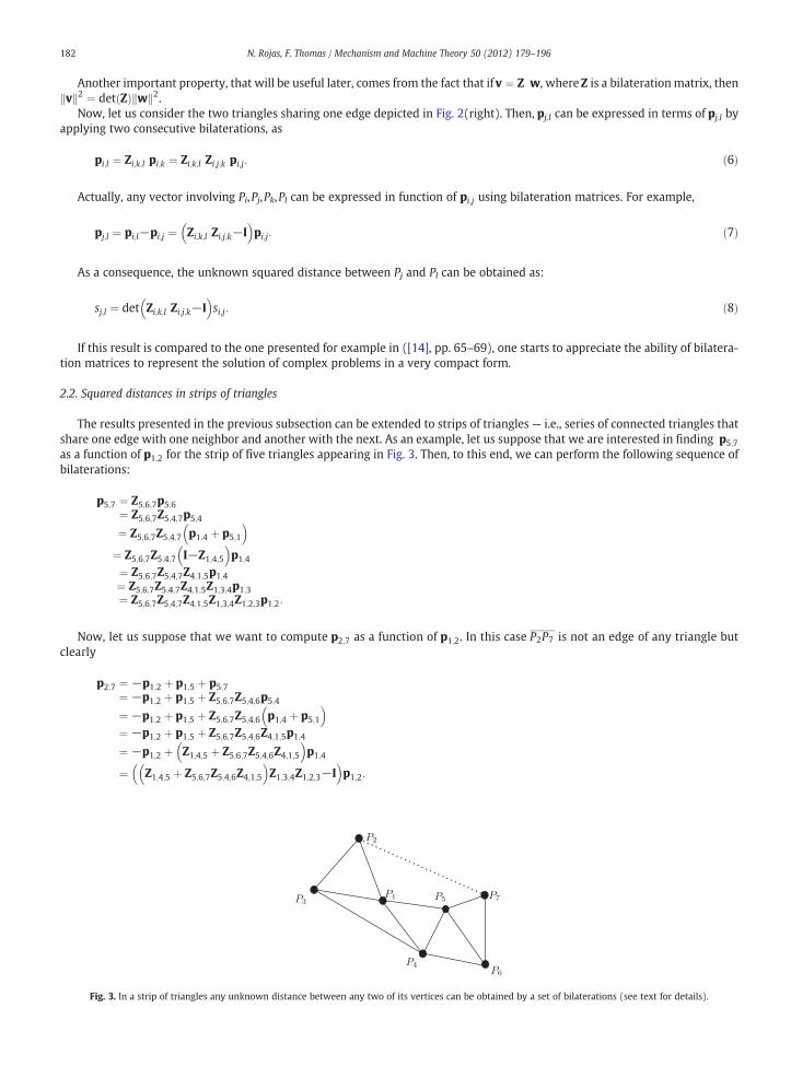
The results presented in the previous subsection can be extended to strips of triangles — i.e., series of connected triangles thatshare one edge with one neighbor and another with the next. As an example, let us suppose that we are interested in finding p5;7as a function of p1;2 for the strip of five triangles appearing in Fig. 3. Then, to this end, we can perform the following sequence ofbilaterations:

p5;7 ¼ Z5;6;7p5;6¼ Z5;6;7Z5;4;7p5;4

¼ Z5;6;7Z5;4;7 p1;4 þ p5;1

� �¼ Z5;6;7Z5;4;7 I−Z1;4;5

� �p1;4

¼ Z5;6;7Z5;4;7Z4;1;5p1;4¼ Z5;6;7Z5;4;7Z4;1;5Z1;3;4p1;3¼ Z5;6;7Z5;4;7Z4;1;5Z1;3;4Z1;2;3p1;2:

Now, let us suppose that we want to compute p2;7 as a function of p1;2. In this case P2P7 is not an edge of any triangle butclearly

p2;7 ¼ −p1;2 þ p1;5 þ p5;7¼ −p1;2 þ p1;5 þ Z5;6;7Z5;4;6p5;4

¼ −p1;2 þ p1;5 þ Z5;6;7Z5;4;6 p1;4 þ p5;1

� �¼ −p1;2 þ p1;5 þ Z5;6;7Z5;4;6Z4;1;5p1;4

¼ −p1;2 þ Z1;4;5 þ Z5;6;7Z5;4;6Z4;1;5

� �p1;4

¼ Z1;4;5 þ Z5;6;7Z5;4;6Z4;1;5

� �Z1;3;4Z1;2;3−I

� �p1;2:

Fig. 3. In a strip of triangles any unknown distance between any two of its vertices can be obtained by a set of bilaterations (see text for details).


Therefore, the squared distance s2, 7 can be expressed, as a function of all other known distance in the strip, as:

s2;7 ¼ det Z1;4;5 þ Z5;6;7Z5;4;6Z4;1;5

� �Z1;3;4Z1;2;3−I

� �s1;2:

Observe that, if s2, 7 is fixed to a given value, the above equation can be seen as a closure equation, a condition that is fulfilled ifand only if the strip of triangles can be assembled so that the distance between P2 and P7 is the desired one. This way of obtainingclosure conditions is extended in the next subsection to complex trusses.

2.3. Closure conditions using bilateration

Fig. 4(a) shows a strip of triangles equivalent to a planar truss consisting of 9 binary links that conforms 4 non-oriented tri-angles. In this truss, once points P1 and P4 have been located on the plane, points P2 and P5 can be positioned in 8 and 4 differentlocations, respectively. If p1;6 is taken as reference, using a sequence of bilaterations, we have that

s2;5 ¼ det I−Z1;3;2Z1;6;3−Z6;4;5Z6;1;4

� �s1;6: ð9Þ

Now, if the binary link P1P6 is removed, the planar truss becomes a four-bar linkage [Fig. 4(b)]. But, if a binary link is thenadded between P2 and P5, a truss is again obtained [Fig. 4(c)]. What are the assembly modes of this new truss? Observe thatthe closure condition of this truss is given by equation (9). The solution of this equation gives the set of values of s1, 6 compatiblewith the lengths of all the binary links of the new truss. Actually, when ΔP1P3P2 and ΔP4P5P6 are oriented –i.e., when ΔP1P3P2 andΔP4P5P6 are ternary links– this truss corresponds to the 5/B1 Baranov truss.

The above process can be iterated further. Considering now that a new triangle is added to the strip of triangles of Fig. 4(a) tothe edge P1P2 , and that points P2 and P5 also belong to another strip of triangles as shown in Fig. 4(d), the result defines a truss inwhich the squared distance s7, 9 can be easily determined. Then, if the binary links P1P6 and P2P5 are removed and a binary link isadded between P7 and P9 a new truss is obtained [Fig. 4(e)]. The assembly modes of this new truss can be computed using theexpression obtained for s7, 9, a scalar equation in s1, 6. Actually, when ΔP1P3P2,ΔP1P2P7, ΔP4P5P6, and ΔP5P9P8 are oriented, theresulting truss corresponds to the 7/B3 Baranov truss.

2.4. Closure conditions and symmetries

The symmetries of a truss are given by its automorphisms. An automorphism of a truss is a set of permutations of its joints thatmap the truss onto itself while preserving the connectivity between joints. The composition of two automorphisms is clearly an-other automorphism, and the set of automorphisms of a given truss, under the composition operation, forms a group, the auto-morphism group of the truss.

a b c

d e

Fig. 4. If the binary link P1P6 is removed in the strip of triangles appearing in (a), a four-bar linkage is obtained (b). If a binary link is then added between P2 and P5,a truss is again obtained (c). The strips of triangles {ΔP1P2P7,ΔP1P3P2,ΔP1P6P3,ΔP1P4P6,ΔP4P5P6} and {ΔP2P5P8,ΔP5P9P8} define a planar truss (d). If the binary linksP1P6 and P2P5 are removed and a binary link is added between P7 and P9 a new truss is obtained whose closure condition can be expressed as the squared distances7, 9 as a function of s1, 6 (e).


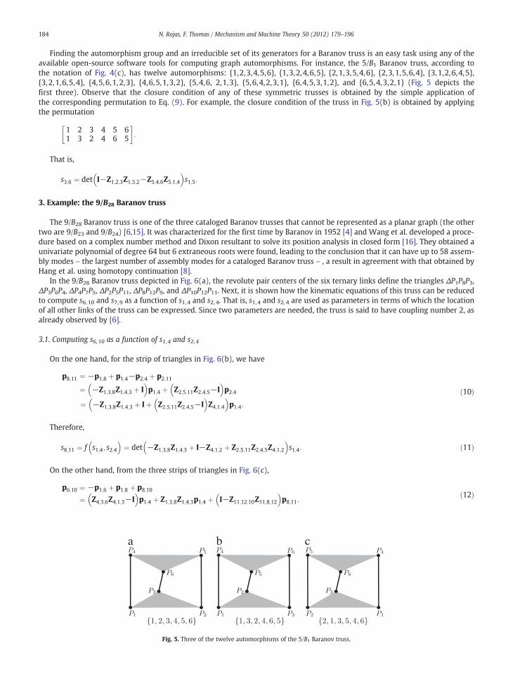
Finding the automorphism group and an irreducible set of its generators for a Baranov truss is an easy task using any of theavailable open-source software tools for computing graph automorphisms. For instance, the 5/B1 Baranov truss, according tothe notation of Fig. 4(c), has twelve automorphisms: {1,2,3,4,5,6}, {1,3,2,4,6,5}, {2,1,3,5,4,6}, {2,3,1,5,6,4}, {3,1,2,6,4,5},{3,2,1,6,5,4}, {4,5,6,1,2,3}, {4,6,5,1,3,2}, {5,4,6, 2,1,3}, {5,6,4,2,3,1}, {6,4,5,3,1,2}, and {6,5,4,3,2,1} (Fig. 5 depicts thefirst three). Observe that the closure condition of any of these symmetric trusses is obtained by the simple application ofthe corresponding permutation to Eq. (9). For example, the closure condition of the truss in Fig. 5(b) is obtained by applyingthe permutation

1 2 3 4 5 61 3 2 4 6 5

� �:

That is,

s3;6 ¼ det I−Z1;2;3Z1;5;2−Z5;4;6Z5;1;4

� �s1;5:

3. Example: the 9/B28 Baranov truss

The 9/B28 Baranov truss is one of the three cataloged Baranov trusses that cannot be represented as a planar graph (the othertwo are 9/B23 and 9/B24) [6,15]. It was characterized for the first time by Baranov in 1952 [4] and Wang et al. developed a proce-dure based on a complex number method and Dixon resultant to solve its position analysis in closed form [16]. They obtained aunivariate polynomial of degree 64 but 6 extraneous roots were found, leading to the conclusion that it can have up to 58 assem-bly modes – the largest number of assembly modes for a cataloged Baranov truss – , a result in agreement with that obtained byHang et al. using homotopy continuation [8].

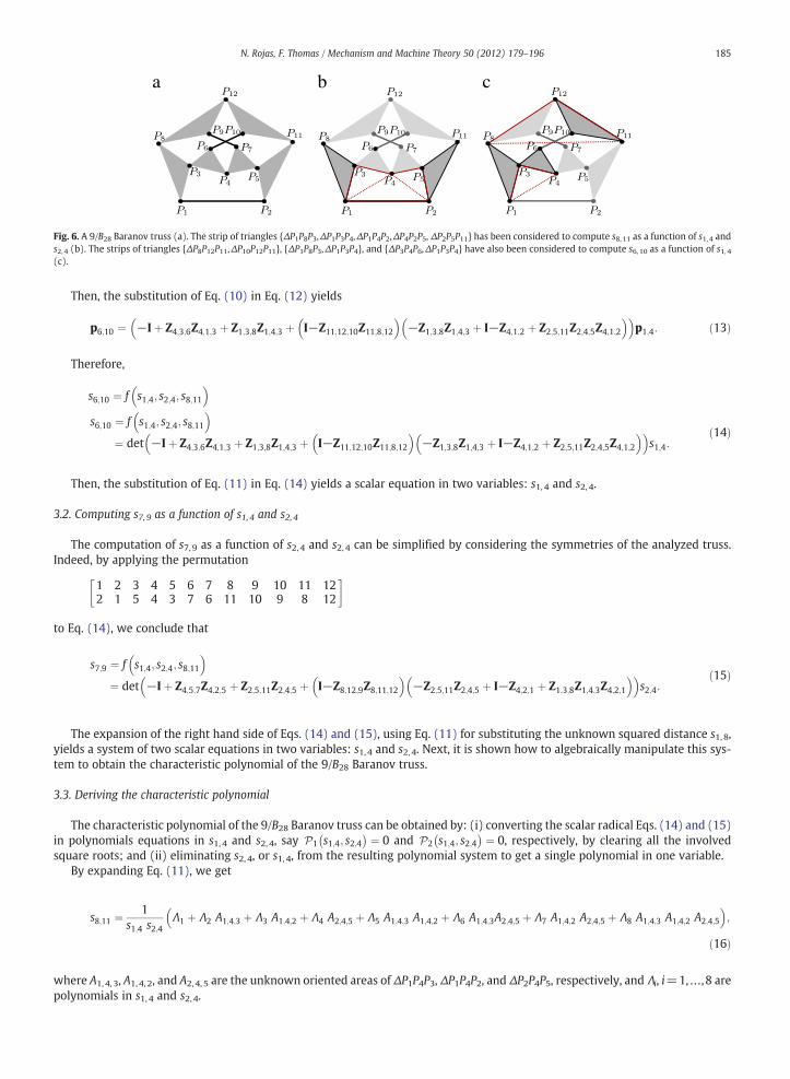
In the 9/B28 Baranov truss depicted in Fig. 6(a), the revolute pair centers of the six ternary links define the triangles ΔP1P8P3,ΔP3P6P4, ΔP4P7P5, ΔP2P5P11, ΔP8P12P9, and ΔP10P12P11. Next, it is shown how the kinematic equations of this truss can be reducedto compute s6, 10 and s7, 9 as a function of s1, 4 and s2, 4. That is, s1, 4 and s2, 4 are used as parameters in terms of which the locationof all other links of the truss can be expressed. Since two parameters are needed, the truss is said to have coupling number 2, asalready observed by [6].

3.1. Computing s6, 10 as a function of s1, 4 and s2, 4

On the one hand, for the strip of triangles in Fig. 6(b), we have

p8;11 ¼ −p1;8 þ p1;4−p2;4 þ p2;11

¼ −Z1;3;8Z1;4;3 þ I� �

p1;4 þ Z2;5;11Z2;4;5−I� �

p2;4

¼ −Z1;3;8Z1;4;3 þ Iþ Z2;5;11Z2;4;5−I� �

Z4;1;4

� �p1;4:

ð10Þ

Therefore,

s8;11 ¼ f s1;4; s2;4� �

¼ det −Z1;3;8Z1;4;3 þ I−Z4;1;2 þ Z2;5;11Z2;4;5Z4;1;2

� �s1;4: ð11Þ

On the other hand, from the three strips of triangles in Fig. 6(c),

p6;10 ¼ −p1;6 þ p1;8 þ p8;10

¼ Z4;3;6Z4;1;3−I� �

p1;4 þ Z1;3;8Z1;4;3p1;4 þ I−Z11;12;10Z11;8;12

� �p8;11:

ð12Þ

a b c

Fig. 5. Three of the twelve automorphisms of the 5/B1 Baranov truss.


Then, the substitution of Eq. (10) in Eq. (12) yields

p6;10 ¼ −Iþ Z4;3;6Z4;1;3 þ Z1;3;8Z1;4;3 þ I−Z11;12;10Z11;8;12

� �−Z1;3;8Z1;4;3 þ I−Z4;1;2 þ Z2;5;11Z2;4;5Z4;1;2

� �� p1;4: ð13Þ

Therefore,

s6;10 ¼ f s1;4; s2;4; s8;11� �

s6;10 ¼ f s1;4; s2;4; s8;11� �

¼ det −Iþ Z4;3;6Z4;1;3 þ Z1;3;8Z1;4;3 þ I−Z11;12;10Z11;8;12

� �−Z1;3;8Z1;4;3 þ I−Z4;1;2 þ Z2;5;11Z2;4;5Z4;1;2

� �� s1;4:

ð14Þ

Then, the substitution of Eq. (11) in Eq. (14) yields a scalar equation in two variables: s1, 4 and s2, 4.

3.2. Computing s7, 9 as a function of s1, 4 and s2, 4

The computation of s7, 9 as a function of s2, 4 and s2, 4 can be simplified by considering the symmetries of the analyzed truss.Indeed, by applying the permutation

1 2 3 4 5 6 7 8 9 10 11 122 1 5 4 3 7 6 11 10 9 8 12

� �

to Eq. (14), we conclude that

s7;9 ¼ f s1;4; s2;4; s8;11� �

¼ det −Iþ Z4;5;7Z4;2;5 þ Z2;5;11Z2;4;5 þ I−Z8;12;9Z8;11;12

� �−Z2;5;11Z2;4;5 þ I−Z4;2;1 þ Z1;3;8Z1;4;3Z4;2;1

� �� s2;4:

ð15Þ

The expansion of the right hand side of Eqs. (14) and (15), using Eq. (11) for substituting the unknown squared distance s1, 8,yields a system of two scalar equations in two variables: s1, 4 and s2, 4. Next, it is shown how to algebraically manipulate this sys-tem to obtain the characteristic polynomial of the 9/B28 Baranov truss.

3.3. Deriving the characteristic polynomial

The characteristic polynomial of the 9/B28 Baranov truss can be obtained by: (i) converting the scalar radical Eqs. (14) and (15)in polynomials equations in s1, 4 and s2, 4, say P1 s1;4; s2;4

�¼ 0 and P2 s1;4; s2;4

�¼ 0, respectively, by clearing all the involved

square roots; and (ii) eliminating s2, 4, or s1, 4, from the resulting polynomial system to get a single polynomial in one variable.By expanding Eq. (11), we get

s8;11 ¼ 1s1;4 s2;4

Λ1 þ Λ2 A1;4;3 þ Λ3 A1;4;2 þ Λ4 A2;4;5 þ Λ5 A1;4;3 A1;4;2 þ Λ6 A1;4;3A2;4;5 þ Λ7 A1;4;2 A2;4;5 þ Λ8 A1;4;3 A1;4;2 A2;4;5

� �;

ð16Þ

where A1, 4, 3, A1, 4, 2, and A2, 4, 5 are the unknown oriented areas of ΔP1P4P3, ΔP1P4P2, and ΔP2P4P5, respectively, and Λi, i=1,…,8 arepolynomials in s1, 4 and s2, 4.

a b c

Fig. 6. A 9/B28 Baranov truss (a). The strip of triangles {ΔP1P8P3,ΔP1P3P4,ΔP1P4P2,ΔP4P2P5, ΔP2P5P11} has been considered to compute s8, 11 as a function of s1, 4 ands2, 4 (b). The strips of triangles {ΔP8P12P11,ΔP10P12P11}, {ΔP1P8P3,ΔP1P3P4}, and {ΔP3P4P6,ΔP1P3P4} have also been considered to compute s6, 10 as a function of s1, 4(c).


Likewise, by expanding Eq. (14), we get

s6;10 ¼ 1s1;4 s2;4 s8;11

Ψ; ð17Þ

where

Ψ ¼ Ψ1 þΨ2A1;4;3 þΨ3A1;4;2 þΨ4A2;4;5 þΨ5A8;11;12 þΨ6A1;4;3A1;4;2 þΨ7A1;4;3

A2;4;5 þΨ8A1;4;3A8;11;12 þΨ9A1;4;2A2;4;5 þΨ10A1;4;2A8;11;12 þΨ11A2;4;5

A8;11;12 þΨ12A1;4;3A1;4;2A2;4;5 þΨ13A1;4;3A1;4;2A8;11;12 þΨ14A1;4;3A2;4;5

A8;11;12 þΨ15A1;4;2A2;4;5A8;11;12 þΨ16A1;4;3A1;4;2A2;4;5A8;11;12;

with Ψi, i=1,…,16, polynomials in s1, 4, s2, 4 and s8, 11.Now, by expressing Eq. (17) as a linear equation in A8, 11, 12 (i.e., a + b A8, 11, 12 =0), squaring it (i.e., a2−b2 A8, 11, 12

2 =0), andreplacing Eq. (16) in the result, a equation in A1, 4, 3, A1, 4, 2, and A2, 4, 5 is obtained. Repeating this process for A2, 4, 5, we get

Φ1 þΦ2 A1;4;3 þΦ3 A1;4;2 þΦ4 A1;4;3 A1;4;2 ¼ 0; ð18Þ

where Φ1, Φ2, Φ3, and Φ4 are polynomials in s1, 4 of degrees 16, 15, 15, and 14, respectively, and in s2, 4 of degree 8 in all cases.Then, to clear radicals, the terms in Eq. (18) can be rearranged to obtain

Φ2 A1;4;3 þΦ3 A1;4;2 ¼ − Φ1 þΦ4 A1;4;3 A1;4;2

� �:

Now, by squaring both sides of the above equation, expanding the result, and rearranging terms, we get

Φ22 A2

1;4;3 þΦ23 A2

1;4;2−Φ24 A2

1;4;3 A21;4;2−Φ2

1 ¼ 2 Φ1 Φ4−Φ2 Φ3ð ÞA1;4;3 A1;4;2:

Finally, if both sides of the above equation are again squared and expanded, the following equation is obtained:

−Φ44A

41;4;3A

41;4;2 þ 2Φ2

4Φ22A

41;4;3A

21;4;2 þ 2Φ2

4Φ23A

21;4;3A

41;4;2−Φ4

2A41;4;3−Φ4

3A41;4;2

−Φ41 þ 2Φ2

2Φ23−8Φ2Φ3Φ4Φ1 þ 2Φ2

4Φ21

� �A21;4;3A

21;4;2 þ 2Φ2

1Φ22A

21;4;3 þ 2Φ2

1Φ23A

21;4;2 ¼ 0:

ð19Þ

If the above procedure is applied to Eq. (16), we get a polynomial in s1, 4, s2, 4, and s8, 11, say F s1;4; s2;4; s8;11 �

. Finally, the fullexpansion of Eq. (19) factorizes as:

s161;4s162;4F s1;4; s2;4;0

� �P1 ¼ 0 ð20Þ

where P1 is a non-homogeneous bivariate polynomial in s1, 4 and s2, 4 with leading term s1, 432 s2, 4

14 . The roots of the terms161;4s

162;4F s1;4; s2;4;0

�were introduced when clearing denominators to obtain Eq. (17), so they can be dropped. To obtain P2, we

can proceed in the same way as for the derivation of P1.Finally, to obtain the characteristic polynomial, we have to eliminate either s2,4 or s1,4 from the polynomial system

P1 s1;4; s2;4 �

¼ 0;P2 s1;4; s2;4 �

¼ 0. This can be implemented using, for example, Sylvester or Bézout resultants. If we eliminateeither s2,4 or s1,4, the associated Sylvester and Bézout matrices have dimensions 68×68 and 36×36, respectively. In any case –i.e.,eliminating either s2,4 or s1,4 and using either Sylvester or Bézout resultants –the result is a polynomial equation of degree 1826.When s2,4 is the eliminated variable, this polynomial factors into 15 polynomials

T s1;4� �

∏14

i¼1Di s1;4

� �¼ 0 ð21Þ


where the roots of polynomials D1;…;D14 are not solutions of the original system of radical equations formed by Eqs. (14) and(15) and T , the characteristic polynomial of the 9/B28 Baranov truss, is of degree 58 in s1, 4. As expected, the same result isobtained when s1, 4 is the eliminated variable.

For each of the real roots of T s1;4 �

¼ 0,we candetermine the Cartesian position of the revolute pair centers given by P2, P4, P5, P6, P7,P9, P10, P11, and P12,with respect to the ternary link given byΔP1P8P3, computing s2,4 from the systemP1 s1;4; s2;4

�¼ 0;P2 s1;4; s2;4

�¼ 0

and using the set of equations

p1;4 ¼ Z1;3;4 p1;3p3;6 ¼ Z3;4;6 p3;4p1;2 ¼ Z1;4;2 p1;4p2;5 ¼ Z2;4;5 p2;4p5;7 ¼ Z4;5;7 p4;5p2;11 ¼ Z2;5;11 p2;5p8;12 ¼ Z8;11;12 p8;11p8;9 ¼ Z8;12;9 p8;12p11;10 ¼ Z11;12;10 p11;12:

This process leads up to 16 combinations of locations for the couples P6, P10 and P7, P9, and at least one of them must satisfysimultaneously the distances imposed by the binary links connecting them.

3.4. Numerical example

According to the notation used in Fig. 6, let us suppose that s1, 2=3185, s1;3 ¼ 66109 , s1;8 ¼ 16525

9 , s2;5 ¼ 8209 , s2;11 ¼ 15826

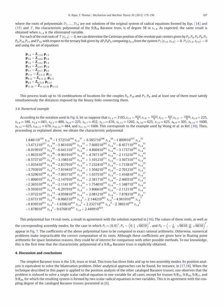
9 , s3, 4=225,s3, 6=180, s3, 8=661, s4, 5=400, s4, 6=225, s4, 7=452, s5, 7=676, s5, 11=1202, s6, 10=625, s7, 9=625, s8, 9=305, s8, 12=1600,s9, 12=625, s10, 11=676, s10, 12=484, and s11, 12=1600. This corresponds to the example used by Wang et al. in Ref. [16]. Then,proceeding as explained above, we obtain the characteristic polynomial

1:848110239 s1;458−1:572510244 s1;4

57 þ 6:585710248 s1;456−1:809910253 s1;4

55

þ3:671210257 s1;454−5:861010261 s1;4

53 þ 7:669210265 s1;452−8:457110269 s1;4

51

þ8:019910273 s1;450−6:641310277 s1;4

49 þ 4:860410281 s1;448−3:173710285 s1;4

47

þ1:863510289 s1;446−9:901910292 s1;4

45 þ 4:787110296 s1;444−2:115210300 s1;4

43

þ8:573710303 s1;442−3:198510307 s1;4

41 þ 1:101210311 s1;440−3:507310314 s1;4

39

þ1:035410318 s1;438−2:837910321 s1;4

37 þ 7:232410324 s1;436−1:715810328 s1;4

35

þ3:793010331 s1;434−7:819410334 s1;4

33 þ 1:504210338 s1;432−2:701210341 s1;4

31

þ4:529610344 s1;430−7:093710347 s1;4

29 þ 1:037510351 s1;428−1:416810354 s1;4

27

þ1:806010357 s1;426−2:147910360 s1;4

25 þ 2:381710363 s1;424−2:460310366 s1;4

23

þ2:365510369 s1;422−2:114110372 s1;4

21 þ 1:754010375 s1;420−1:348710378 s1;4

19

þ9:593010380 s1;418−6:297910383 s1;4

17 þ 3:806610386 s1;416−2:112110389 s1;4

15

þ1:072210392 s1;414−4:959810394 s1;4

13 þ 2:081210397 s1;412−7:878310399 s1;4

11

þ2:673110402 s1;410−8:066510404 s1;4

9 þ 2:144210407 s1;48−4:961010409 s1;4

7

þ9:839510411 s1;46−1:639610414 s1;4

5 þ 2:232710416 s1;44−2:386510418 s1;4

3

þ1:878010420 s1;42−9:676810421 s1;4 þ 2:449910423

:

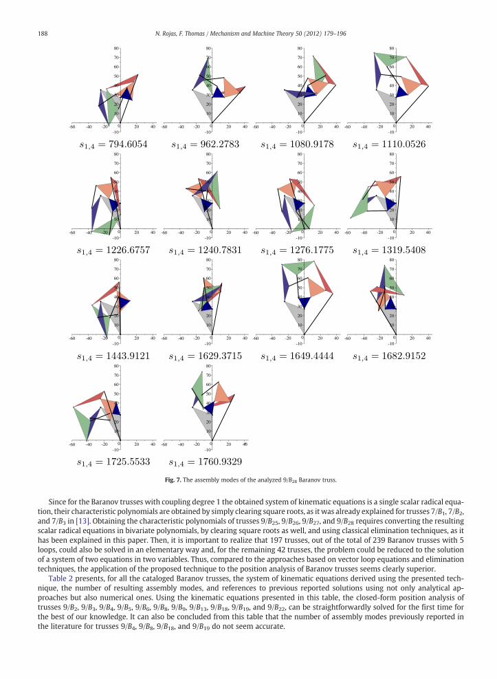
This polynomial has 14 real roots, a result in agreement with the solution reported in [16]. The values of these roots, as well as

the corresponding assembly modes, for the case in which P1=(0,0)T, P3 ¼ 0; 13ffiffiffiffiffiffiffiffiffiffiffi6610

p� �T, and P8 ¼ − 3

10

ffiffiffiffiffiffiffiffiffiffiffi6610

p; 1330

ffiffiffiffiffiffiffiffiffiffiffi6610

p� �T,

appear in Fig. 7. The coefficients of the above polynomial have to be computed in exact rational arithmetic. Otherwise, numericalproblems make impracticable the correct computation of its roots. Although these coefficients are given here in floating pointarithmetic for space limitation reasons, they could be of interest for comparison with other possible methods. To our knowledge,this is the first time that the characteristic polynomial of a 9/B28 Baranov truss is explicitly obtained.

4. Discussion and conclusions

The simplest Baranov truss is the 3/B1 truss or triad. This truss has three links and up to two assembly modes. Its position anal-ysis is equivalent to solve the bilateration problem. Other analytical approaches can be found, for instance, in [17,18]. When thetechnique described in this paper is applied to the position analysis of the other cataloged Baranov trusses, one observes that theproblem is reduced to solve a single scalar radical equation in one variable for all cases, except for trusses 9/B25, 9/B26, 9/B27, and9/B28, for which the resulting system is formed by two scalar radical equations in two variables. This is in agreement with the cou-pling degree of the cataloged Baranov trusses presented in [6].


Since for the Baranov trusses with coupling degree 1 the obtained system of kinematic equations is a single scalar radical equa-tion, their characteristic polynomials are obtained by simply clearing square roots, as it was already explained for trusses 7/B1, 7/B2,and 7/B3 in [13]. Obtaining the characteristic polynomials of trusses 9/B25, 9/B26, 9/B27, and 9/B28 requires converting the resultingscalar radical equations in bivariate polynomials, by clearing square roots as well, and using classical elimination techniques, as ithas been explained in this paper. Then, it is important to realize that 197 trusses, out of the total of 239 Baranov trusses with 5loops, could also be solved in an elementary way and, for the remaining 42 trusses, the problem could be reduced to the solutionof a system of two equations in two variables. Thus, compared to the approaches based on vector loop equations and eliminationtechniques, the application of the proposed technique to the position analysis of Baranov trusses seems clearly superior.

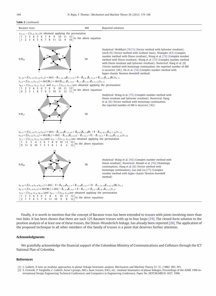
Table 2 presents, for all the cataloged Baranov trusses, the system of kinematic equations derived using the presented tech-nique, the number of resulting assembly modes, and references to previous reported solutions using not only analytical ap-proaches but also numerical ones. Using the kinematic equations presented in this table, the closed-form position analysis oftrusses 9/B2, 9/B3, 9/B4, 9/B5, 9/B6, 9/B8, 9/B9, 9/B13, 9/B18, 9/B19, and 9/B22, can be straightforwardly solved for the first time forthe best of our knowledge. It can also be concluded from this table that the number of assembly modes previously reported inthe literature for trusses 9/B4, 9/B8, 9/B18, and 9/B19 do not seem accurate.

-60 -40 -20-10

20 400

10

20

30

40

50

60

70

80

-60 -40 -20-10

20 400

10

20

30

40

50

60

70

80

-60 -40 -20-10

20 400

10

20

30

40

50

60

70

80

-60 -40 -20-10

20 400

10

20

30

40

50

60

70

80

-60 -40 -20-10

20 400

10

20

30

40

50

60

70

80

-60 -40 -20-10

20 400

10

20

30

40

50

60

70

80

-60 -40 -20-10

20 400

10

20

30

40

50

60

70

80

-60 -40 -20-10

20 400

10

20

30

40

50

60

70

80

-60 -40 -20-10

20 400

10

20

30

40

50

60

70

80

-60 -40 -20-10

20 400

10

20

30

40

50

60

70

80

-60 -40 -20-10

20 400

10

20

30

40

50

60

70

80

-60 -40 -20-10

20 400

10

20

30

40

50

60

70

80

-60 -40 -20-10

20 400

10

20

30

40

50

60

70

80

-60 -40 -20-10

20 400

10

20

30

40

50

60

70

80

Fig. 7. The assembly modes of the analyzed 9/B28 Baranov truss.


Table 2Position analysis of all the cataloged Baranov trusses.

Baranov truss AM Reported solutions

5/B1 6

Analytical: Peisach [21], Pennock and Kassner [22], Gosselin et al. [23,24], Wohlhart[25], Husty [26], Kong and Gosselin [27], Collins [28] (Basic elimination theory),Han et al. [29], Liu et al. [30], Luo [31] (Wu method), Rojas and Thomas [32,33](Bilateration method). Numerical: Hang et al. [8] (Vector method with homotopycontinuation), Luo et al. [34] (Newton iterative method), Chandra and Rolland[35] (Hybrid metaheuristics)

s2, 5= f(s1, 6)=det(I−Z1, 3, 2Z1, 6, 3−Z6, 4, 5 Z6, 1, 4)s1, 6

7/B1 14

Analytical: Kong and Yang [36], Innocenti [37] (Vector method with Sylvesterresultant), Dhingra et al. [38] (Vector method with Sylvester resultant), Rojasand Thomas [13] (Bilateration method). Numerical: Liu and Yang [39] (Homotopycontinuation), Hang et al. [8] (Vector method with homotopy continuation)

s5, 8= f(s1, 4,s6, 7)=det(−Z1, 3, 5Z1, 4, 3+ I−Z4, 3, 6 Z4, 1, 3+Z6, 9, 8Z6, 7, 9Ω1)s1, 4s6, 7= f(s1, 4)=det(Ω1)=det(Z4, 3, 6Z4, 1, 3−Z4, 2, 7Z4, 1, 2)s1, 4

7/B2 16

Analytical: Innocenti [40] (Vector method with an ad-hoc elimination procedure),Almadi et al. [41] (Vector method with Sylvester resultant), Dhingra et al. [38](Vector method with Sylvester resultant), Dhingra et al. [42] (Vector methodwith Gröbner basis and Sylvester resultant), Wampler [43] (Complex numbermethod with Dixon resultant), Rojas and Thomas [13] (Bilateration method).Numerical: Hang et al. [8] (Vector method with homotopy continuation),Shen et al. [44] (Single-opened-chains iterative method)

s1, 6= f(s4, 7,s3, 8)=det(−Z3, 2, 1Z3, 8, 2Ω1−Z4, 5, 3Z4, 7, 5+Z4, 9, 6Z4, 7, 9)s4, 7s3, 8= f(s4, 7)=det(Ω1)=det(−Z4, 5, 3Z4, 7, 5+ I−Z7, 9, 8Z7, 4, 9)s4, 7

7/B3 18

Analytical: Innocenti [45,46] (Vector method with Sylvesterresultant), Han et al. [47] (Complex number method with Sylvesterresultant), Dhingra et al. [38] (Vector method with Sylvesterresultant), Wang et al. [48] (Complex number method withWu method), Ni et al. [49] (Conformal geometric algebra withDixon resultant), Rojas and Thomas [13] (Bilateration method).Numerical: Hang et al. [8] (Vector method with homotopycontinuation)

s7, 9= f(s1, 6,s2, 5)=det((Z1, 3, 2−Z1, 3, 7)Z1, 6, 3+(I−Z5, 8, 9 Z5, 2, 8)Ω1)s1, 6s2, 5= f(s1, 6)=det(Ω1)=det(−Z1, 3, 2Z1, 6, 3+ I−Z6, 4, 5Z6, 1, 4)s1, 6

9/B1 54Analytical: Lösch [9] (Vector method with Gröbner basis), Dhingraet al. [50] (Vector method with Gröbner basis), Wei et al. [51](Complex number method with Sylvester resultant), Wohlhart[52] (Vector method with Sylvester resultant). Numerical: Hang et al.[8] (Vector method with homotopy continuation)

s5, 12= f(s1, 7,s3, 8,s4, 10)=det(Z4, 1, 5Z1, 3, 4Z1, 2, 3Z1, 7, 2+(I−Z10, 11, 12 Z10, 4, 11)Ω2)s1, 7s4, 10= f(s1, 7,s3, 8)=det(Ω2)=det(−Z1, 3, 4Z1, 2, 3Z1, 7, 2+Z1, 2, 3Z1, 7, 2+(I−Z8, 9, 10Z8, 3, 9)Ω1)s1, 7s3, 8= f(s1, 7)=det(Ω1)=det(−Z1, 2, 3Z1, 7, 2+ I−Z7, 6, 8Z7, 1, 6)s1, 7

9/B2 54 Numerical: Hang et al. [8] (Vector method with homotopycontinuation)

s10, 12= f(s1, 7, s3, 8,s4, 11)=det(−Z1, 2, 3Z1, 7, 2−(I−Z8, 9, 10Z8, 3, 9)Ω1+Z1, 3, 4Z1, 2, 3Z1, 7, 2+Z4, 5, 12Z4, 11, 5Ω2)s1, 7s4, 11= f(s1, 7,s3, 8)=det(Ω2)=det(−Z1, 3, 4Z1, 2, 3Z1, 7, 2+Z1, 2, 3Z1, 7, 2+(I−Z8, 9, 11Z8, 3, 9)Ω1)s1, 7s3, 8= f(s1, 7)=det(Ω1)=det(−Z1, 2, 3Z1, 7, 2+ I−Z7, 6, 8Z7, 1, 6)s1, 7

(continued on next page)


Unlabelled image

Unlabelled image

Unlabelled image

Unlabelled image

Unlabelled image

Table 2 (continued)


9/B3 48

Numerical: Hang et al. [8] (Vector methodwith homotopy continuation)

s8, 9= f(s1, 12,s3, 10,s2, 6)=det(−Z1, 4, 3Z1, 12, 4−(I−Z10, 7, 6Z10, 3, 7)Ω1+Z6, 5, 8Z6, 2, 5Ω2+ I−Z12, 11, 9Z12, 1, 11)s1, 12s2, 6= f(s1, 12,s3, 10)=det(Ω2)=det(−Z1, 4, 2Z1, 12, 4+Z1, 4, 3Z1, 12, 4+(I−Z10, 7, 6Z10, 3, 7)Ω1)s1, 12s3, 10= f(s1, 12)=det(Ω1)=det(−Z1, 4, 3Z1, 12, 4+ I−Z12, 11, 10Z12, 1, 11)s1, 12

9/B4 42 Numerical: Hang et al. [8] (Vector method with homotopycontinuation, the reported number of AM is incorrect (38))

s6, 7= f(s1, 12,s3, 10,s2, 9)=det(−Z1, 4, 2Z1, 12, 4−Z2, 5, 6Z2, 9, 5Ω2+Z1, 4, 3Z1, 12, 4

+Z3, 8, 7Z3, 10, 8Ω1)s1, 12s2, 9= f(s1, 12)=det(Ω2)=det(−Z1, 4, 2Z1, 12, 4+ I−Z12, 11, 9Z12, 1, 11)s1, 12s3, 10= f(s1, 12)=det(Ω1)=det(−Z1, 4, 3Z1, 12, 4+ I−Z12, 11, 10Z12, 1, 11)s1, 12

9/B5 48Numerical: Hang et al. [8] (Vector methodwith homotopy continuation)

s6, 7= f(s1, 12,s3, 10,s2, 9)=det(−Z1, 4, 2Z1, 12, 4−Z2, 5, 6Z2, 9, 5Ω2+Z1, 4, 3Z1, 12, 4+(I−Z10, 8, 7Z10, 3, 8)Ω1)s1, 12s2, 9= f(s1, 12)=det(Ω2)=det(−Z1, 4, 2Z1, 12, 4+ I−Z12, 11, 9Z12, 1, 11)s1, 12s3, 10= f(s1, 12)=det(Ω1)=det(−Z1, 4, 3Z1, 12, 4+ I−Z12, 11, 10Z12, 1, 11)s1, 12

9/B6 48 Numerical: Hang et al. [8] (Vector method withhomotopy continuation)

s4, 12= f(s7, 9,s2, 6,s3, 10)=det((−Z2, 3, 4+ I)Z2, 1, 3Z2, 6, 1Ω1+(I−Z10, 11, 12Z10, 3, 11)Ω2)s7, 9s3, 10= f(s7, 9,s2, 6)=det(Ω2)=det(Z9, 5, 2Z9, 7, 5−Z2, 1, 3Z2, 6, 1Ω1−Z9, 8, 10Z9, 7, 8)s7, 9s2, 6= f(s7, 9)=det(Ω1)=det(− I+Z9, 5, 2Z9, 7, 5+Z7, 8, 6Z7, 9, 8)s7, 9

9/B7 48 Analytical: Han et al. [53] (Complex number method withSylvester resultant). Numerical: Hang et al. [8] (Vectormethod with homotopy continuation)

s4, 12= f(s1, 5,s6, 9,s3, 10)=det(−Z1, 3, 4Z1, 2, 3Z1, 5, 2+Z1, 2, 3Z1, 5, 2+(I−Z10, 11, 12Z10, 3, 11)Ω2)s1, 5s3, 10= f(s1, 5,s6, 9)=det(Ω2)=det(−Z1, 2, 3Z1, 5, 2+Z1, 7, 6Z1, 5, 7+(I−Z9, 8, 10Z9, 6, 8)Ω1)s1, 5s6, 9= f(s1, 5)=det(Ω1)=det(−Z1, 7, 6Z1, 5, 7+ I−Z5, 2, 9Z5, 1, 2)s1, 5

9/B8 48Numerical: Hang et al. [8] (Vector method with homotopycontinuation, the reported number of AM is incorrect (44))

s4, 12= f(s1, 7,s5, 8,s3, 10)=det(−Z1, 3, 4Z1, 2, 3Z1, 7, 2+Z1, 2, 3Z1, 7, 2+(I−Z10, 11, 12Z10, 3, 11)Ω2)s1, 7


Unlabelled image

Unlabelled image

Unlabelled image

Unlabelled image

Unlabelled image

Unlabelled image

Table 2 (continued)


s3, 10= f(s1, 7,s5, 8)=det(Ω2)=det(−Z1, 2, 3Z1, 7, 2+ I−Z7, 2, 5Z7, 1, 2+(I−Z8, 9, 10Z8, 5, 9)Ω1)s1, 7s5, 8= f(s1, 7)=det(Ω1)=det(Z7, 2, 5Z7, 1, 2−Z7, 6, 8Z7, 1, 6)s1, 7


s4, 12= f(s1, 7,s6, 8,s3, 10)=det(−Z1, 3, 4Z1, 2, 3Z1, 7, 2+Z1, 2, 3Z1, 7, 2+(I−Z10, 11, 12Z10, 3, 11)Ω2)s1, 7s3, 10= f(s1, 7,s6, 8)=det(Ω2)=det(−Z1, 2, 3Z1, 7, 2+ I−Z7, 5, 6Z7, 1, 5+(I− fZ8, 9, 10Z8, 6, 9)Ω1)s1, 7s6, 8= f(s1, 7)=det(Ω1)=det(− I+Z7, 5, 6Z7, 1, 5+Z1, 5, 8Z1, 7, 5)s1, 7

9/B1030

Analytical: Han et al. [54] (Complex number method with Sylvesterresultant), Dhingra et al. [55] (Vector method with Sylvesterresultant), Borràs and Di Gregorio [56] (Vector method withSylvester dialytic elimination method). Numerical: Liu and Yang[39] (Homotopy continuation), Hang et al. [8] (Vector method withhomotopy continuation), Cai et al. [57]

s11, 12= f(s1, 3, s5, 7,s8, 10)=det(−Z1, 7, 10Z1, 4, 7Z1, 3, 4+Z10, 9, 11Z10, 8, 9Ω2+Z1, 2, 12Z1, 3, 2)s1, 3s8, 10= f(s1, 3,s5, 7)=det(Ω2)=det(−Z1, 4, 7Z1, 3, 4+Z7, 6, 8Z7, 5, 6Ω1+Z1, 7, 10Z1, 4, 7Z1, 3, 4)s1, 3s5, 7= f(s1, 3)=det(Ω1)=det(Z1, 4, 7Z1, 3, 4− I+Z3, 4, 5Z3, 1, 4)s1, 3

9/B11 36

Analytical: Wei et al. [58] (Complex number method with Sylvesterresultant). Numerical: Hang et al. [8] (Vector method with homotopycontinuation, the reported number of AM is incorrect (34))

s11, 12= f(s1, 3, s5, 7,s8, 10)=det(−Z1, 7, 10Z1, 4, 7Z1, 3, 4+(I−Z8, 9, 11Z8, 10, 9)Ω2+Z1, 2, 12Z1, 3, 2)s1, 3s8, 10= f(s1, 3,s5, 7)=det(Ω2)=det(−Z1, 4, 7Z1, 3, 4+Z7, 6, 8Z7, 5, 6Ω1+Z1, 7, 10Z1, 4, 7Z1, 3, 4)s1, 3s5, 7= f(s1, 3)=det(Ω1)=det(Z1, 4, 7Z1, 3, 4− I+Z3, 4, 5Z3, 1, 4)s1, 3

9/B12 40

Analytical: Dhingra et al. [55] (Vector method with Sylvesterresultant). Numerical: Hang et al. [8] (Vector method withhomotopy continuation, the reported number of AM isincorrect, (54))

s2, 3= f(s4, 6,s8, 10,s1, 11)=det(−Z4, 7, 1Z4, 6, 7−Z1, 12, 2Z1, 11, 12Ω2+ I−Z6, 5, 3Z6, 4, 5)s4, 6s1, 11= f(s4, 6,s8, 10)=det(Ω2)=det(−Z4, 7, 1Z4, 6, 7+ I−Z6, 7, 8Z6, 4, 7+Z8, 9, 11Z8, 10, 9Ω1)s4, 6s8, 10= f(s4, 6)=det(Ω1)=det(− I+Z6, 7, 8Z6, 4, 7+Z4, 7, 10Z4, 6, 7)s4, 6

9/B13 40

Numerical: Hang et al. [8] (Vector method with homotopy continuation)

s8, 11= f(s2, 4,s6, 7,s10, 12)=det(Z4, 3, 6Z4, 2, 3−Z6, 9, 8Z6, 7, 9Ω1−Z4, 1, 10Z4, 2, 1+(I−Z12, 5, 11Z12, 10, 5)Ω2)s2, 4s10, 12= f(s2, 4, s6, 7)=det(Ω2)=det(− I+Z4, 1, 10Z4, 2, 1+Z2, 1, 12Z2, 4, 1)s2, 4s6, 7= f(s2, 4)=det(Ω1)=det(Z4, 3, 6Z4, 2, 3−Z4, 1, 7Z4, 2, 1)s2, 4

9/B14 42

Analytical: Han et al. [59] (Complex number method with Sylvesterresultant). Numerical: Hang et al. [8] (Vector method with homotopycontinuation, the reported number of AM is incorrect (52))

s2, 3= f(s4, 6,s10, 11,s1, 12)=det(−Z4, 7, 1Z4, 6, 7−(I−Z12, 9, 2Z12, 1, 9)Ω2+ I−Z6, 5, 3Z6, 4, 5)s4, 6



Unlabelled image

Unlabelled image

Unlabelled image

Unlabelled image

Unlabelled image

Unlabelled image

Table 2 (continued)


s1, 12= f(s4, 6,s10, 11)=det(Ω2)=det(−Z4, 7, 1Z4, 6, 7+Z4, 7, 10Z4, 6, 7+(I−Z11, 8, 12Z11, 10, 8)Ω1)s4, 6s10, 11= f(s4, 6)=det(Ω1)=det(−Z4, 7, 10Z4, 6, 7+ I−Z6, 7, 11Z6, 4, 7)s4, 6

9/B15 52Analytical: Dhingra et al. [55] (Vector method with Sylvester resultant),Numerical: Hang et al. [8] (Vector method with homotopy continuation,the reported number of AM is incorrect (26))

s3, 6= f(s10, 11, s1, 12, s2, 4)=det(−Z10, 7, 1Z10, 11, 7−(I−Z12, 9, 2Z12, 1, 9)Ω1−Z2, 5, 3Z2, 4, 5Ω2+ I−Z11, 7, 6Z11, 10, 7)s10, 11s2, 4= f(s10, 11, s1, 12)=det(Ω2)=det(−Z10, 7, 1Z10, 11, 7−(I−Z12, 9, 2Z12, 1, 9)Ω1+ I−Z10, 7, 4Z11, 10, 7)s10, 11s1, 12= f(s10, 11)=det(Ω1)=det(−Z10, 7, 1Z10, 11, 7+ I−Z11, 8, 12Z11, 10, 8)s10, 11

9/B16 44 Analytical: Han et al. [60] (Complex number method with Sylvesterresultant). Numerical: Hang et al. [8] (Vector method with homotopycontinuation)

s2, 3= f(s7, 8,s4, 6, s1, 11)=det(−Z7, 10, 1Z7, 8, 10−Z1, 12, 2Z1, 11, 12Ω2+Z7, 10, 4Z7, 8, 10+(I−Z6, 5, 3Z6, 4, 5)Ω1)s7, 8s1, 11= f(s7, 8,s4, 6)=det(Ω2)=det(−Z7, 10, 1Z7, 8, 10+ I−Z8, 10, 11Z8, 7, 10)s7, 8s4, 6= f(s7, 8)=det(Ω1)=det(−Z7, 10, 4Z7, 8, 10+ I−Z8, 9, 6Z8, 7, 9)s7, 8

9/B17 44Analytical: Han et al. [61] (Complex number method with Sylvesterresultant). Numerical: Hang et al. [8] (Vector method with homotopycontinuation, the reported number of AM is incorrect (66))

s3, 6= f(s1, 2,s10, 12,s7, 8)=det(− I+Z2, 4, 3Z2, 1, 4+Z1, 4, 7Z1, 2, 4+(I−Z8, 9, 6Z8, 7, 9)Ω2)s1, 2s7, 8= f(s1, 2,s10, 12)=det(Ω2)=det(−Z1, 4, 7Z1, 2, 4+Z1, 4, 10Z1, 2, 4+Z10, 11, 8Z10, 12, 11Ω1)s1, 2s10, 12= f(s1, 2)=det(Ω1)=det(−Z1, 4, 10Z1, 2, 4+ I−Z2, 5, 12Z2, 1, 5)s1, 2


s11, 12= f(s1, 4, s6, 7,s5, 9)=det(−Z1, 3, 5Z1, 4, 3−(I−Z9, 8, 11Z9, 5, 8)Ω2+ I−Z4, 3, 6Z4, 1, 3+(I−Z7, 10, 12Z7, 6, 10)Ω1)s1, 4s5, 9= f(s1, 4,s6, 7)=det(Ω2)=det(−Z1, 3, 5Z1, 4, 3+ I−Z4, 3, 6Z4, 1, 3+Z6, 10, 9Z6, 7, 10Ω1)s1, 4s6, 7= f(s1, 4)=det(Ω1)=det(Z4, 3, 6Z4, 1, 3−Z4, 2, 7Z4, 1, 2)s1, 4


s11, 12= f(s1, 4, s6, 7,s5, 9)=det(−Z1, 3, 5Z1, 4, 3−Z5, 8, 11Z5, 9, 8Ω2+ I−Z4, 3, 6Z4, 1, 3+(I−Z7, 10, 12Z7, 6, 10)Ω1)s1, 4s5, 9= f(s1, 4,s6, 7)=det(Ω2)=det(−Z1, 3, 5Z1, 4, 3+ I−Z4, 3, 6Z4, 1, 3+Z6, 10, 9Z6, 7, 10Ω1)s1, 4s6, 7= f(s1, 4)=det(Ω1)=det(Z4, 3, 6Z4, 1, 3−Z4, 2, 7Z4, 1, 2)s1, 4

9/B20 46

Analytical: Wang et al. [62] (Complex number method withDixon resultant and Sylvester resultant), Wang et al. [63](Complex number method with Sylvester resultant). Numerical:Hang et al. [8] (Vector method with homotopy continuation,the reported number of AM is incorrect (64)), Luo and Liu [64](Complex number method with chaos least square method)

s5, 6= f(s1, 4,s8, 11,s9, 10)=det(− I+Z4, 3, 5Z4, 1, 3+Z1, 3, 8Z1, 4, 3+Z8, 12, 9Z8, 11, 12Ω1+(I−Z10, 7, 6Z10, 9, 7)Ω2)s1, 4


Unlabelled image

Unlabelled image

Unlabelled image

Unlabelled image

Unlabelled image

Unlabelled image

Table 2 (continued)


s9, 10= f(s1, 4,s8, 11)=det(Ω2)=det((−Z8, 12, 9Z8, 11, 12+ I−Z11, 12, 10Z11, 8, 12)Ω1)s1, 4s8, 11= f(s1, 4)=det(Ω1)=det(−Z1, 3, 8Z1, 4, 3+ I−Z4, 2, 11Z4, 1, 2)s1, 4

9/B21 40

Analytical: Wang et al. [65] (Complex number methodwith Dixon resultant and Sylvester resultant). Numerical:Hang et al. [8] (Vector method with homotopy continuation,the reported number of AM is incorrect (30))

s5, 8= f(s1, 4,s6, 11,s7, 12)=det(−Z1, 3, 5Z1, 4, 3+ I−Z4, 3, 6Z4, 1, 3+Z6, 10, 7Z6, 11, 10Ω1+(I−Z12, 9, 8Z12, 7, 9)Ω2)s1, 4s7, 12= f(s1, 4,s6, 11)=det(Ω2)=det((−Z6, 10, 7Z6, 11, 10+ I−Z11, 10, 12Z11, 6, 10)Ω1)s1, 4s6, 11= f(s1, 4)=det(Ω1)=det(Z4, 3, 6Z4, 1, 3−Z4, 2, 11Z4, 1, 2)s1, 4


s7, 10= f(s1, 4,s8, 11,s5, 9)=det(− I+Z4, 3, 5Z4, 1, 3−Z5, 6, 7Z5, 9, 6Ω2+Z1, 3, 8Z1, 4, 3+(I−Z11, 12, 10Z11, 8, 12)Ω1)s1, 4s5, 9= f(s1, 4,s8, 11)=det(Ω2)=det(− I+Z4, 3, 5Z4, 1, 3+Z1, 3, 8Z1, 4, 3+Z8, 12, 9Z8, 11, 12Ω1)s1, 4s8, 11= f(s1, 4)=det(Ω1)=det(−Z1, 3, 8Z1, 4, 3+ I−Z4, 2, 11Z4, 1, 2)s1, 4

9/B23 46

Analytical: Zhuang et al. [66] (Complex number methodwith Sylvester resultant), Wang et al. [67] (Complex numbermethod with Dixon resultant and Sylvester resultant).Numerical: Hang et al. [8] (Vector method with homotopycontinuation)

s10, 11= f(s1, 4, s6, 8,s5, 7)=det(−Z6, 12, 10Z6, 8, 12Ω1−Z1, 3, 6Z1, 4, 3+Z1, 2, 5Z1, 4, 2+Z5, 9, 11Z5, 7, 9Ω2)s1, 4s5, 7= f(s1, 4,s6, 8)=det(Ω2)=det(−Z1, 2, 5Z1, 4, 2+ I−Z4, 3, 7Z4, 1, 3)s1, 4s6, 8= f(s1, 4)=det(Ω1)=det(−Z1, 3, 6Z1, 4, 3+ I−Z4, 2, 8Z4, 1, 2)s1, 4

9/B24 50

Analytical: Wang et al. [68] (Complex number method with Dixon resultantand Sylvester resultant). Numerical: Hang et al. [8] (Vector method withhomotopy continuation)

s7, 11= f(s1, 4,s6, 8,s5, 10)=det(− I+Z4, 3, 7Z4, 1, 3+Z1, 2, 5Z1, 4, 2+(I−Z10, 9, 11Z10, 5, 9)Ω2)s1, 4s5, 10= f(s1, 4,s6, 8)=det(Ω2)=det(−Z1, 2, 5Z1, 4, 2+Z1, 3, 6Z1, 4, 3+Z6, 12, 10Z6, 8, 12Ω1)s1, 4s6, 8= f(s1, 4)=det(Ω1)=det(−Z1, 3, 6Z1, 4, 3+ I−Z4, 2, 8Z4, 1, 2)s1, 4

9/B25 52 Analytical: Wang et al. [69] (Complex number method with Dixon resultantand Sylvester resultant). Numerical: Hang et al. [8] (Vector method withhomotopy continuation)

s9;10 ¼ f s1;6; s2;7 �

¼ det −Iþ Z6;5;9Z6;1;5 þ Z1;3;2Z1;6;3 þ I−Z7;8;10Z7;2;8 �

Z2;4;7 −Z1;3;2Z1;6;3 þ Z1;3;4Z1;6;3 � �

s1;6



Unlabelled image

Unlabelled image

Unlabelled image

Unlabelled image

Unlabelled image

Finally, it is worth to mention that the concept of Baranov truss has been extended to trusses with joints involving more thantwo links. It has been shown that there are such 125 Baranov trusses with up to four loops [19]. The closed-form solution to theposition analysis of at least one of these trusses, the Dixon–Wunderlich linkage, has already been reported [20]. The application ofthe proposed technique to all other members of this family of trusses is a point that deserves further attention.

Acknowledgments

We gratefully acknowledge the financial support of the Colombian Ministry of Communications and Colfuturo through the ICTNational Plan of Colombia.

References

[1] C. Galletti, A note on modular approaches to planar linkage kinematic analysis, Mechanism and Machine Theory 21 (5) (1986) 385–391.[2] E. Ceresole, P. Fanghella, C. Galletti, Assur's groups, AKCs, basic trusses, SOCs, etc.: modular kinematics of planar linkages, Proceedings of the ASME 1996 In-

ternational Design Engineering Technical Conferences and Computers in Engineering Conference, Paper No. DETC96/MECH-1027, 1996.

Table 2 (continued)


s11;12 ¼ f s1;6; s2;7 �

is obtained applying the permutation1 2 3 4 5 6 7 8 9 10 11 121 2 3 4 5 6 7 8 11 12 9 10

� �to the above equation

9/B26 56

Analytical: Wohlhart [70,71] (Vector method with Sylvester resultant),Lösch [9] (Vector method with Gröbner basis), Wampler [43] (Complexnumber method with Dixon resultant), Wang et al. [72] (Complex numbermethod with Dixon resultant), Wang et al. [73] (Complex number methodwith Dixon resultant and Sylvester resultant). Numerical: Hang et al. [8](Vector method with homotopy continuation, the reported number of AMis incorrect (38)), He et al. [74] (Complex number method withhyper-chaotic Newton downhill method)

s5, 10= f(s3, 11, s3, 12, s1, 4)=det(−Z11, 12, 10Z11, 3, 12+ I−Z3, 6, 1Z3, 11, 6+Z1, 2, 5Z1, 4, 2Ω1)s3, 11s1, 4= f(s3, 11,s3, 12)=det(Ω1)=det(Z3, 6, 1Z3, 11, 6−Z3, 7, 4Z3, 12, 7Z3, 11, 12)s3, 11s8;9 ¼ f s3;12; s3;11; s1;4

�and s1;4 ¼ f s3;12; s3;11

�are obtained applying the permutation

1 2 3 4 5 6 7 8 9 10 11 124 2 3 1 8 7 6 5 10 9 12 11

� �to the above equations

9/B27 50

Analytical: Wang et al. [75] (Complex number method withDixon resultant and Sylvester resultant). Numerical: Hanget al. [8] (Vector method with homotopy continuation,the reported number of AM is incorrect (36))

s9, 11= f(s5, 12, s7, 12, s3, 6)=det(−Z7, 10, 6Z7, 12, 10+Z6, 8, 9Z6, 3, 8Ω1+ I−Z12, 10, 11Z12, 7, 10)s7, 12s3, 6= f(s5, 12,s7, 12)=det(Ω1)=det(−Z5, 4, 3Z5, 12, 4(−Z7, 12, 5+ I)−Z7, 12, 5+Z7, 10, 6Z7, 12, 10)s7, 12s1;2 ¼ f s7;12; s5;12; s3;6

�and s3;6 ¼ f s7;12; s5;12


1 2 3 4 5 6 7 8 9 10 11 129 11 6 10 7 3 5 8 1 4 2 12


9/B28 58

Analytical: Wang et al. [16] (Complex number method withDixon resultant). Numerical: Almadi et al. [76] (Homotopycontinuation), Hang et al. [8] (Vector method withhomotopy continuation), Luo and Liu [77] (Complexnumber method with hyper-chaotic Newton downhillmethod)

s6, 10= f(s1, 4,s2, 4,s8, 11)=det(− I+Z4, 3, 6Z4, 1, 3+Z1, 3, 8Z1, 4, 3+(I−Z11, 12, 10Z11, 8, 12)Ω1)s1, 4s8, 11= f(s1, 4,s2, 4)=det(Ω1)=det(−Z1, 3, 8Z1, 4, 3+ I−Z4, 1, 2+Z2, 5, 11Z2, 4, 5Z4, 1, 2)s1, 4s7;9 ¼ f s2;4; s1;4; s8;11

�and s8;11 ¼ f s2;4; s1;4


1 2 3 4 5 6 7 8 9 10 11 122 1 5 4 3 7 6 11 10 9 8 12



Unlabelled image

Unlabelled image

Unlabelled image

[3] E. Peisach, On Assur groups, Baranov trusses, Grübler chains, planar linkages and on their structural (number) synthesis, The 22th Working Meeting of theIFToMM Permanent Commission for Standardization of Terminology, LaMCoS - INSA de LYON, Villeurbanne, France, 2008, pp. 33–41.

[4] G. Baranov, Classification, formation, kinematics, and kinetostatics of mechanisms with pairs of the first kind (in Russian), Proceedings of Seminar on theTheory of Machines and Mechanisms, Moscow, Vol. 2, 1952, pp. 15–39.

[5] N. Manolescu, T. Erdelean, La determination des fermes Baranov avec e=9 elements en utilisant la methode de graphisation inverse, paper d-12, Proceed-ings of the 3rd IFToMM World Congress on the Theory of Machines and Mechanisms, September, Kupari, Yugoslavia, Vol. D, 1971, pp. 177–188.

[6] T. Yang, F. Yao, Topological characteristics and automatic generation of structural synthesis of planar mechanisms based on the ordered single-opened-chains, Proceedings of ASME 1994 Mechanisms Conference, Vol. 70, 1994, pp. 67–74.

[7] N. Manolescu, A method based on Baranov trusses, and using graph theory to find the set of planar jointed kinematic chains and mechanisms, Mechanismand Machine Theory 8 (1) (1973) 3–22.

[8] L. Hang, Q. Jin, J. Wu, T. Yang, A general study of the number of assembly configurations for multi-circuit planar linkages, Journal of Southeast University(English edition) 16 (1) (2000) 46–51.

[9] S. Lösch, Parallel redundant manipulators based on open and closed normal Assur chains, in: J. Merlet, B. Ravani (Eds.), Computational Kinematics, KluverAcademic Publishers, 1995, pp. 251–260.

[10] K. Wohlhart, Position analyses of open normal Assur groups a(3.6), ASME/IFToMM International Conference on Reconfigurable Mechanisms and Robots,2009, pp. 88–94.

[11] N. Rojas, F. Thomas, Closed-form solution to the position analysis of Watt–Baranov trusses using the bilateration method, Journal of Mechanisms and Robot-ics 3 (3) (2011) 031001.

[12] T. Yang, Structural analysis and number synthesis of spatial mechanisms, Proceedings of the 6th IFToMM World Congress on the Theory of Machines andMechanisms, December 15–20, New Delhi, India, Vol. 1, 1983, pp. 280–283.

[13] N. Rojas, F. Thomas, Distance-based position analysis of the three seven-link Assur kinematic chains, Mechanism and Machine Theory 46 (2) (2011) 112–126.[14] J. Graver, Counting on frameworks: mathematics to aid the design of rigid structures, The Mathematical Association of America, 2001.[15] H. Shen, T. Yang, A numerical method and automatic generation for determining the assemblage configurations of complex planar linkages based on the

ordered SOCs, Proceedings of ASME 1996 Design Engineering Technical Conferences and Computers in Engineering Conference, Paper No. 96-DETC/MECH-1030, 1996.

[16] P. Wang, Q. Liao, S. Wei, Y. Zuang, Direct position analysis of nine-link Barranov truss based on Dixon resultant, Journal of Beijing University of Aeronauticsand Astronautics 32 (7) (2006) 852–855 864.

[17] C. Suh, C. Radcliffe, Kinematics and Mechanism Design, Wiley, New York, 1978.[18] C. Galletti, On the position analysis of Assur's groups of high class, Meccanica 14 (1979) 6–10.[19] J. Chu, W. Cao, T. Yang, Type synthesis of Baranov truss with multiple joints and multiple-joint links, Proceedings of ASME 1998 Design Engineering Tech-

nical Conferences and Computers in Engineering Conference, Paper No. DETC98/MECH-5972, 1998.[20] D. Walter, M. Husty, On a nine-bar mechanism, its possible configurations and conditions for flexibility, Proceedings of the 12th IFToMM World Congress in

Mechanism and Machine Science, June 17–20, Besançon, France, 2007.[21] E. Peisach, Determination of the position of the member of three-joint and two-joint four member Assur groups with rotational pairs (in Russian), Machi-

nowedenie 5 (1985) 55–61.[22] G. Pennock, D. Kassner, Kinematic analysis of a planar eight-bar linkage: application to a platform-type robot, Journal of Mechanical Design 114 (1) (1992)

87–95.[23] C. Gosselin, J. Sefrioui, Polynomial solutions for the direct kinematic problem of planar three-degree-of-freedom parallel manipulators, Fifth International

Conference on Advanced Robotics, ‘Robots in Unstructured Environments’, ICAR, vol. 2, 1991, pp. 1124–1129.[24] C. Gosselin, J. Sefrioui, M. Richard, Solutions polynomiales au problème de la cinématique des manipulateurs parallèles plans à trois degrés de liberté, Mech-

anism and Machine Theory 27 (2) (1992) 107–119.[25] K. Wohlhart, Direct kinematic solution of a general planar Stewart platform, Proceedings of the International Conference on Computer Integrated

Manufacturing, Zakopane, Poland, 1992, pp. 403–411.[26] M. Husty, Kinematic mapping of planar three-legged platforms, Proceedings of 15th Canadian Congress of Applied Mechanics (CANCAM 1995), Vol. 2, 1995,

pp. 876–877.[27] X. Kong, C. Gosselin, Forward displacement analysis of third-class analytic 3-RPR planar parallel manipulators, Mechanism and Machine Theory 36 (9)

(2001) 1009–1018.[28] C. Collins, Forward kinematics of planar parallel manipulators in the Clifford algebra of p2, Mechanism and Machine Theory 37 (8) (2002) 799–813.[29] L. Han, Y. Zhang, C. Liang, Wu's method for forward displacement analysis of the planar parallel mechanisms, Journal of Beijing University of Aeronautics and

Astronautics 24 (1) (1998) 116–119.[30] H. Liu, T. Zhang, H. Ding, Forward solutions of the 3-RPR planar parallel mechanism with Wu's method, Journal of Beijing Institute of Technology 20 (5)

(2000) 565–569.[31] Y. Luo, Forward solutions of the 3-RPR planar parallel mechanism with Wu's method, Journal of Hunan University of Arts and Science (Science and Technol-

ogy) 2 (2004) 27–29.[32] N. Rojas, F. Thomas, A robust forward kinematics analysis of 3-RPR planar platforms, 12th International Symposium on Advances in Robot Kinematics, 2010,

pp. 23–32.[33] N. Rojas, F. Thomas, The forward kinematics of 3-RPR planar robots: a review and a distance-based formulation, IEEE Transactions on Robotics 27 (1) (2011)

143–150.[34] Y. Luo, X. Li, L. Luo, D. Liao, The research of Newton iterative method based on chaos mapping and its application to forward solutions of the 3-RPR planar

parallel mechanism, Machine Design and Research 23 (2) (2007) 37–39.[35] R. Chandra, L. Rolland, On solving the forward kinematics of 3RPR planar parallel manipulator using hybrid metaheuristics, Applied Mathematics and Com-

putation In Press, Corrected Proof.[36] X. Kong, T. Yang, Closed-form displacement analysis of 3-loop Baranov trussed, Proceedings of International Conference on Spatial Mechanisms and High

Class Mechanisms (Theory and Practice), 1994.[37] C. Innocenti, Position analysis in analytical form of the 7-link Assur kinematic chain featuring one ternary link connected to ternary links only, Mechanism

and Machine Theory 32 (4) (1997) 501–509.[38] A. Dhingra, A. Almadi, D. Kohli, Closed-form displacement analysis of 8, 9 and 10-link mechanisms: Part I: 8-link 1-DOF mechanisms, Mechanism and Ma-

chine Theory 35 (6) (2000) 821–850.[39] A. Liu, T. Yang, Displacement analysis of planar complex mechanisms using continuation method, Mechanical Science and Technology 13 (2) (1994) 55–62.[40] C. Innocenti, Analytical-form position analysis of the 7-link Assur kinematic chain with four serially-connected ternary links, Journal of Mechanical Design

116 (2) (1994) 622–628.[41] A. Almadi, A. Dhingra, D. Kohli, Closed-form displacement analysis of SDOF 8 link mechanisms, Proceedings of ASME 1996 Design Engineering Technical

Conferences and Computers in Engineering Conference, Paper No. 96-DETC/MECH-1206, 1996.[42] A. Dhingra, A. Almadi, D. Kohli, A Gröbner–Sylvester hybrid method for closed-form displacement analysis of mechanisms, Journal of Mechanical Design 122

(4) (2000) 431–438.[43] C. Wampler, Solving the kinematics of planar mechanisms by Dixon determinant and a complex-plane formulation, Journal of Mechanical Design 123 (3)

(2001) 382–387.[44] H. Shen, K. Ting, T. Yang, Configuration analysis of complex multiloop linkages and manipulators, Mechanism and Machine Theory 35 (3) (2000) 353–362.[45] C. Innocenti, Analytical determination of the intersections of two coupler-point curves generated by two four-bar linkages, in: J. Angeles, G. Hommel, P.

Kovács (Eds.), Computational Kinematics, Kluwer Academic Publishers, Dordrecht, the Netherlands, 1993, pp. 251–262.


[46] C. Innocenti, Polynomial solution to the position analysis of the 7-link Assur kinematic chain with one quaternary link, Mechanism and Machine Theory 30(8) (1995) 1295–1303.

[47] L. Han, Q. Liao, C. Liang, The closed form displacement analysis of a seven-link Barranov-truss and all the Assur groups connected with it, Mechanical Scienceand Technology 17 (5) (1998) 785–788.

[48] P. Wang, Q. Liao, S. Wei, Forward displacement analysis of a seven-link Barravo truss based on Wu method, Mechanical Science and Technology 25 (6)(2006) 748–752.

[49] Z. Ni, Q. Liao, S. Wei, New research of forward displacement analysis of 6-link Assur group, 2nd International Conference on Information Science and Engi-neering (ICISE), 2010, pp. 5187–5190.

[50] A. Dhingra, A. Almadi, D. Kohli, Closed-form displacement and coupler curve analysis of planar multi-loop mechanisms using Gröbner bases, Mechanism andMachine Theory 36 (2) (2001) 273–298.

[51] S. Wei, X. Zhou, Q. Liao, Research on assembly configurations for nine-link Barranov truss, Mechanical Science and Technology 23 (8) (2004) 962–965.[52] K. Wohlhart, Robots based on Assur group a(3.5), in: J. Lenarcic, P. Wenger (Eds.), Advances in Robot Kinematics: Analysis and Design, Springer, Nether-

lands, 2008, pp. 165–175.[53] L. Han, Q. Liao, C. Liang, Closed-form displacement analysis for a nine-link Barranov truss or a eight-link Assur group, Mechanism and Machine Theory 35 (3)

(2000) 379–390.[54] L. Han, Q. Liao, C. Liang, A kind of algebraic solution for the position analysis of a planar basic kinematic chain, Journal of Machine Design 16 (3) (1999)

16–18.[55] A. Dhingra, A. Almadi, D. Kohli, Closed-form displacement analysis of 10-link 1-DOF mechanisms: Part 2 — polynomial solutions, Mechanism and Machine

Theory 36 (1) (2001) 57–75.[56] J. Borràs, R.D. Gregorio, Polynomial solution to the position analysis of two Assur kinematic chains with four loops and the same topology, Journal of Mech-

anisms and Robotics 1 (2) (2009) 021003.[57] S. Cai, Y. Zuo, N. Chen, Position analysis of planar complex mechanisms using triangular vector loop method, Journal of Lanzhou University of Technology 31

(5) (2005) 35–38.[58] S. Wei, X. Zhou, Q. Liao, Closed-form displacement analysis of one kind of nine-link Barranov trusses, Proceedings of the 11th IFToMM World Congress in

Mechanism and Machine Science, April 1–4, Tianjin, China, 2004, pp. 1176–1177.[59] L. Han, Q. Liao, C. Liang, Closed-form displacement analysis of a planar fifth-class group with lower pairs, Journal of Beijing University of Aeronautics and

Astronautics 24 (5) (1998) 603–606.[60] L. Han, Q. Liao, C. Liang, Closed-form displacement analysis of an eight links planer Assur group, Proceedings of the 10th World Congress on the Theory of

Machine and Mechanisms, June 20–24, Oulu, Finland, 1999, pp. 168–173.[61] L. Han, Q. Liao, C. Liang, Complex number method for kinematic analysis of planar Assur groups, Mechanical Science and Technology 17 (3) (1998) 410–412.[62] P. Wang, Q. Liao, Y. Zhuang, S. Wei, Direct position analysis of a nine-link Barranov truss, Journal of Tsinghua University (Science and Technology) 46 (8)

(2006) 1373–1376.[63] P. Wang, Q. Liao, S. Wei, Y. Zhuang, Displacement analysis of a kind of nine-link Barranov truss, Journal of Beijing University of Posts and Telecommunica-

tions 29 (3) (2006) 12–17.[64] Y. Luo, Q. Liu, Forward displacement analysis of 25th nine-link Barranov truss based on chaos least square method, 2nd International Conference on Com-

puter Modeling and Simulation (ICCMS), Vol. 1, 2010, pp. 184–188.[65] P. Wang, Q. Liao, Z. Lu, Displacement analysis of a nine-link Barranov truss, Machine Design and Research 25 (2) (2009) 33–36.[66] Y. Zhuang, P. Wang, Q. Liao, Research on displacement analysis of a kind of non-planar nine link Barranov truss, Journal of Beijing University of Posts and

Telecommunications 29 (6) (2006) 13–16.[67] P. Wang, L. Wang, D. Li, J. Gu, J. Song, Closed-form displacement analysis of a kind of non-planar nine-link Barranov truss, IEEE International Conference on

Automation and Logistics, ICAL, 2008, pp. 2397–2401.[68] P. Wang, Q. Liao, Z. Lu, Displacement analysis of non-planar nine-link Barranov truss, Journal of Beijing University of Posts and Telecommunications 31 (4)

(2008) 10–14.[69] P. Wang, Q. Liao, Y. Zuang, S. Wei, Displacement analysis of nine-link Barranov truss, Chinese Journal of Mechanical Engineering 43 (7) (2007) 11–15.[70] K. Wohlhart, Position analysis of the rhombic Assur group 4.4, Proceedings of the RoManSy, CISM-IFTOMM Symposium, Gdansk, Poland, 1994, pp. 21–31.[71] K. Wohlhart, Position analyses of normal quadrilateral Assur groups, Mechanism and Machine Theory 45 (9) (2010) 1367–1384.[72] P. Wang, Q. Liao, S. Wei, Y. Zuang, Forward displacement analysis of a kind of nine-link Barranov truss based on Dixon resultants, China Mechanical Engi-

neering 17 (21) (2006) 2034–2038.[73] P. Wang, Q. Liao, Y. Zhuang, S. Wei, A method for position analysis of a kind of nine-link Barranov truss, Mechanism and Machine Theory 42 (10) (2007)

1280–1288.[74] Z. He, Y. Luo, Q. Liu, Forward displacement analysis of a kind of nine-link Barranov truss based on hyper-chaotic Newton downhill method, 2nd International

Conference on Intelligent Human-Machine Systems and Cybernetics (IHMSC), Vol. 2, 2010, pp. 137–142.[75] P. Wang, Q. Liao, Y. Zhuang, S. Wei, Research on position analysis of a kind of nine-link Barranov truss, Journal of Mechanical Design 130 (1) (2008) 011005.[76] A. Almadi, A. Dhingra, D. Kohli, Displacement analysis of ten-link kinematic chains using homotopy, Proceedings of 9th World Congress on Theory of

Machines and Mechanisms, Vol. 1, 1995, pp. 90–94.[77] Y. Luo, Q. Liu, Forward displacement analysis of non-plane two coupled degree nine-link Barranov truss based on hyper-chaotic Newton downhill method,

Applied Mechanics and Materials 20–23 (2010) 659–664.


Documents

On closed-form solutions to the position analysis of Baranov trusses