Embed Size (px)
Citation preview

Journal of Algebra 236, 502–521 (2001)doi:10.1006/jabr.2000.8516, available online at http://www.idealibrary.com on
On Bounding the Number of Generators for Fat PointIdeals on the Projective Plane
Stephanie Fitchett
Honors College, Florida Atlantic University, Jupiter, Florida 33458
Communicated by Craig Huneke
Received July 8, 1999
Let X be the surface obtained by blowing up general points p1� � � � � pn of the pro-jective plane over an algebraically closed ground field k, and let L be the pullbackto X of a line on the plane. If C is a rational curve on X with C · L = d, then forevery t there is a natural map ��C��C�t�� ⊗ ��X��X�L�� → ��C��C�t + d�� givenby multiplication on simple tensors. The ranks of such maps are determined as afunction of t, d, and m, where m is the largest multiplicity of C at any of the pointspi. If I is the ideal defining the fat point subscheme Z = m1p1 + · · · +mnpn ⊂ P2,and α is the least degree in which I has generators, then the ranks of the maps��C��C�t�� ⊗ ��X��X�L�� → ��C��C�t + d�� can be used for bounding the num-ber of generators of I in degrees t > α+ 1. © 2001 Academic Press
1. INTRODUCTION
A basic concern in algebraic geometry is understanding the relationshipbetween a subscheme of projective space and the homogeneous ideal ofpolynomials which defines the subscheme. This work employs geometricmethods to investigate the relationship between the geometry of fat pointsubschemes of the projective plane and the structure of their defining ide-als. Given distinct points p1� � � � � pn in P2 (the projective plane over analgebraically closed field k), and positive integer multiplicities m1� � � � �mn,let Z denote the fat point subscheme Z = m1p1 + · · · +mnpn. Its corre-sponding homogeneous ideal I = IZ in the coordinate ring kx� y� z of P2
is I = Pm11 ∩ · · · ∩ Pmnn , where Pi is the saturated homogeneous ideal defin-
ing the point pi. The ideal I is called a fat point ideal, and consists of thehomogeneous polynomials in three variables which, for each i, vanish toorder at least mi at pi.
502
0021-8693/01 $35.00Copyright © 2001 by Academic PressAll rights of reproduction in any form reserved.

generators for fat point ideals 503
Although the scheme Z = m1p1 + · · · + mnpn ⊂ P2 looks reasonablysimple, understanding its ideal I can be difficult. Being homogeneous, I is adirect sum I = ⊕t≥0It of its homogeneous components It of degree t. Mostinvestigations of such fat point ideals follow one of two lines of restriction:limiting the possible number n of points, or restricting the multiplicitiesm1� � � � �mn.In both cases, we first seek an understanding of the Hilbert function of
I (i.e., the k-dimension of the vector space It as a function of t), and thenmove to the number of generators. Harbourne [H1] and Hirschowitz [Hi]have conjectured values for the Hilbert function, and the conjectured valueshave been verified for many cases. (See, for example, [AH, H1, Hi, CM1,CM2]; [Mi] offers a nice survey.) In particular, the conjectured values holdfor ideals defining fat point subschemes supported at nine or fewer generalpoints of the projective plane (see [N, H5]).This note begins at the next natural step: for the cases in which the con-
jectured values of the Hilbert function hold, we wish to determine, for eacht, the number νt�I� of elements of degree t in a minimal set of homoge-neous generators for I. It turns out that νt�I� just measures how much of Itis not in the span of the products of elements of It−1 with x, y, and z. Moreprecisely, νt�I� is the k-dimension of cokernel of the natural multiplicationmap µt−1� It−1 ⊗k �x� y� z� → It .Our general understanding of numbers of generators for fat point ideals
is still fairly limited. Investigations have followed the previously mentionedlines of inquiry, involving restrictions on the number n of points ([Cat, H2]for five or fewer general points; [F2] for six general points, [H4] for sevengeneral points; [FHH] for eight general points) or on the multiplicitiesinvolved ([GCR] for uniform multiplicity 1; [H3] for uniform multiplicitieslarger than 1). Here we use a method which is independent of both thenumber of points and the size of the multiplicities to bound νt�I� for t >α+ 1, where α is the smallest degree r such that Ir �= 0. In fact, we showthat under relatively mild hypotheses νt�I� for t > α + 1 is controlled bythe geometry of Iα.This geometry becomes most apparent by working on the surface X
obtained by blowing up the points p1� � � � � pn. For each graded com-ponent It of I, there is an associated line bundle �t in the Picardgroup of X. Under natural identifications I = ⊕t≥0It = ⊕t≥0��X��t�,and µt−1� It−1 ⊗k �x� y� z� → It is µFt−1 � ��X��t−1� ⊗ ��X��� →��X��t�, where � denotes the global section functor, and � is theline bundle associated to the pullback to X of a line on P2. Thus,for a fat point ideal, determining the number νt of generators indegree t is equivalent to finding the dimension of the cokernel of��X��t−1� ⊗ ��X��� → ��X��t�. This note uses geometric tools tobound the ranks of maps µF � ��X��X�F�� ⊗ ��X��� → ��X��X�F� ⊗��

504 stephanie fitchett
for effective divisors F on X, a situation which encompasses the cases ofinterest for fat point ideals.The second section contains background material and preliminary results
needed for working on the blow-up surface X. Proposition 2.1 shows howinformation about the rank of µF can be obtained from information abouta similar map on sections of the restriction of F to a curve C on X, andinduction.In Section 3, we determine the ranks of natural multiplication maps
��C��C�t�� ⊗ ��X��X�L�� → ��C��C�t + d���where L is the pullback to X of a line on P2, and C is a rational curveon X with C · L = d (Theorem 3.1). This result is then used to determinebounds on the cokernels of the maps
��X��X�rC + L�� ⊗ ��X��X�L�� → ��X��X�rC + 2L���where 0 ≤ r ≤ d (Theorem 3.3). The theorem shows that the boundsdepend on both d and the maximum multiplicity m of a point on the imageof C in P2. In particular, when d −m and m differ by at most one, andnotably in the case of rational curves C on blow-ups of P2 at eight or fewerpoints, Corollary 3.4 shows that the cokernel of
��X��X�rC + L�� ⊗ ��X��X�L�� → ��X��X�rC + 2L��is(r−min�d�d−m�
2
)-dimensional.
The final section shows how Theorem 3.3 can be used to bound thenumber of elements νt of degree t in a minimal generating set for a fatpoint ideal, for all t > α+ 1. Finally, in Theorem 4.4, the bounds obtainedusing Theorem 3.3 are shown to be at least as good as the bounds due toCampanella [Cam], which were previously the best known.This article is partially based on results in my thesis [F1], and I wish to
express my sincere appreciation to my advisor, Brian Harbourne, for histime, patience, and many helpful discussions.
2. PRELIMINARIES
Let X be the surface obtained by blowing up general points p1� � � � � pnof P2. If π� X → P2 is the blow-up map, for each 1 ≤ i ≤ n, we let Eidenote the exceptional divisor π−1�pi�, and let L denote the pullback toX of a line on P2. Recall that −L2 = E2
1 = · · ·E2n = −1, and L · Ei = 0,
for all i. Also, the bundles associated to L, E1� � � � � En form a basis for thePicard group of X.

generators for fat point ideals 505
We begin with a useful proposition of Mumford’s. Recall that if X is aclosed subscheme of projective space, then for any two coherent sheaves �and � on X, there is a natural map
��X�� � ⊗ ��X��� µ−→ ��X�� ⊗���given by multiplication on simple tensors. We will always take � to be thesheaf associated to the pullback L to X of a line on P2, and we will denotethe kernel and cokernel of the map µ by R�� � and S�� �, respectively. Welet s�� � denote dimk S�� �.Proposition 2.1. Let X be a closed subscheme of projective space, let
� and � be coherent sheaves on X, and let � be the sheaf associated to aneffective Cartier divisor C on X. If the restriction homomorphisms ��X�� � →��C�� ⊗ �C� and ��X�� ⊗�� → ��C�� ⊗� ⊗ �C� are surjective, then wehave an exact sequence
0 → R�� ⊗ �−1� → R�� � → R�� ⊗ �C�→ S�� ⊗ �−1� → S�� � → S�� ⊗ �C� → 0�
Proof. This is the 6-lemma in [Mu].
Note that if I is the fat point ideal defining Z = m1p1 + · · · +mnpn, andI = ⊕t≥0��X��t�, then νt = s��t−1� for all t. Thus we take the geomet-ric point of view and study maps of line bundles. Recall that a divisor isnumerically effective if it meets every effective divisor non-negatively.
Definition. Let F be an effective divisor on the blow-up X of P2 atpoints p1� � � � � pn. A decomposition
F = H +N�where H is an effective, numerically effective divisor, h0�X��X�H�� =h0�X��X�F��, and N is the divisor which consists of the components ofnegative self-intersection in the fixed locus of the linear system �F �, is calleda Zariski decomposition of F . If � = �X�F�, � = �X�H�, and � = �X�N�,we will also call
� = � ⊗ �
a Zariski decomposition for � .
Our definition specializes more general definitions (see, for example,[Cu, Mo], or the original work of Zariski [Z]) to the case of divisorson blow-up surfaces. Also, the standard definition for a Zariski decom-position requires only that H is effective, numerically effective, and hash0�X��X�H�� = h0�X��X�F��. Our concerte specification for N makesthe Zariski decomposition unique.We take the time to point out a couple of simple facts which we will need
later.
506 stephanie fitchett
Lemma 2.2. Let F = H + N be the Zariski decomposition of an effec-tive divisor F on X, and assume N = ∑q
i=1 riCi, where each Ci is a dis-tinct exceptional curve (i.e., a smooth rational curve of self-intersection −1).Then
(a) Ci · Cj = 0 for all i �= j, and(b) H · Ci = 0 for all 1 ≤ i ≤ q.
Proof. To see (a), note that Ci · Cj ≥ 0 for any two distinct exceptionalcurves Ci and Cj , and if Ci · Cj > 0, then �Ci + Cj� has no base locus, andthus cannot be part of N . Similarly, for part (b), H · Ci ≥ 0 for all i, and ifH · Ci > 0, then Ci is not a fixed component of H + Ci.In order to compute the Zariski decomposition of F , we must be able
to determine that F is effective, and we need to be able to identify all thecurves of negative self-intersection on X which may occur in N . FollowingHarbourne, we give a name to fat point subschemes having the necessaryproperties.
Definition. Let Z = m1p1 + · · · +mnpn be a fat point subscheme ofP2 with mi > 0 for all i. For each t let Ft denote the divisor tL−m1E1 −· · · −mnEn on the surface X obtained by blowing up p1� � � � � pn. Let α bethe smallest value of t for which h0�X��X�Ft�� > 0 (i.e., the smallest t suchthat Ft is linearly equivalent to an effective divisor). Assume Fα = H +N isthe Zariski decomposition for Fα. We will say Z is expectedly good providedh1�X��X�H�� = 0 and the components of N are exceptional curves. Wewill also say the points p1� � � � � pn are expectedly good provided the onlyprime divisors on X of negative self-intersection are exceptional curves,and h1�X��X�C�� = 0 for every effective, numerically effective divisorC on X.
If F = H + N is the Zariski decomposition of F , the conditionh1�X��X�H�� = 0 allows us to compute h0�X��X�F�� by using thefact that h0�X��X�F�� = h0�X��X�H�� = �H2 −K ·H�/2 + 1 (Riemann–Roch).Any nine general points are known to be expectedly good, and conjec-
tures put forth by Harbourne [H1] and Hirschowitz [Hi] imply that anynumber of general points will be expectedly good. Note that to check thatthe subscheme Z is expectedly good, we need only verify that the compo-nents of N are exceptional curves, and check that h1 of the bundle associ-ated to a single numerically effective divisor is 0. Thus it is often possibleto show that a subscheme Z is expectedly good, even if we do not knowthat the points in the support of Z are expectedly good.The following fact shows that if Z is an expectedly good fat point sub-
scheme supported at p1� � � � � pn, and I = ⊕��X��t� is its defining ideal,

generators for fat point ideals 507
then we can determine s��t� for all t provided we can determine s��� forevery bundle � associated to a numerically effective divisor on X, whereX is the blow-up of P2 at p1� � � � � pn.
Lemma 2.3 [H2, Lemma 2.10]. If F is an effective divisor with Zariskidecomposition F = H + N , then s��X�F�� = s��X�H�� + h0�X��X�F +L�� − h0�X��X�H + L��.The final two lemmas of this section show that for t ≥ α + 1� s��t� is
controlled by the geometry of the fixed part of �t−1.
Lemma 2.4. Suppose F is an effective divisor onX and assume the Zariskidecomposition of � = �X�F� is � = � ⊗ � , where � is the sheaf associatedto a numerically effective divisor H, h1�X��� = 0, and � is the sheaf asso-ciated to a sum of exceptional curves. Let � = �X�L�. Then s�� ⊗ � � =s�� ⊗ � �N� = s�� ⊗ � �, where N is the effective divisor with associatedsheaf � .
Proof. Apply Proposition 2.1 using � ⊗ � ⊗ � for � and � for �. Weget
0 → R�� ⊗ �� → R�� ⊗ � ⊗ � � → R�� ⊗ � ⊗ � �N�→ S�� ⊗ �� → S�� ⊗ � ⊗ � � → S�� ⊗ � ⊗ � �N� → 0�
Since h1�X��� = 0, S�� ⊗ �� = 0 by [DGM, Proposition 3.7], so S�� ⊗� ⊗ � � ∼= S�� ⊗ � ⊗ � �N�.Since H ·N = 0 for every effective divisor H whose associated sheaf is
isomorphic to � , we have � ⊗� ⊗ � �N ∼= � ⊗ � �N and �⊗2 ⊗� ⊗ � �N ∼=�⊗2 ⊗� �N . Therefore S�� ⊗� ⊗� �N� ∼= S�� ⊗� �N�, which gives the firstequality. Also, since S��� = 0, the exact sequence S��� → S�� ⊗ � � →S�� ⊗ � �N� → 0 forces S�� ⊗ � � ∼= S�� ⊗ � �N�, yielding the secondequality.
The next lemma shows that because the Ci’s which appear in N aredisjoint, studying s�� ⊗ � �N� can be reduced to studying s�� ⊗ �
⊗rii �riCi�
for various Ci and ri.
Lemma 2.5. Let X be the blow-up of P2 at points p1� � � � � pn. If � =⊗qi=1�⊗ri
i , where each �i in the line bundle associated to an exceptional divisorCi, Ci · Cj = 0 for all i �= j, and ri ≤ L · Ci, then s�� ⊗ � �N� =
∑qi=1 s�� ⊗
�⊗rii �riCi�.Proof. Since N is the disjoint sum
∑qi=1 riCi, we have s�� ⊗ � �N� =∑q
i=1 s�� ⊗ � �riCi�, but � ⊗ � �riCi ∼= � ⊗ �⊗ri �riCi , and the resultfollows.

508 stephanie fitchett
Assume � = � ⊗ � is the Zariski decomposition of the line bundle �of an effective divisor and � corresponds to some component of an idealwhich defines an expectedly good fat point subscheme. The isomorphismsin the previous lemmas give a string of dimension equalities:
s�� ⊗ � ⊗ � � = s�� ⊗ � �N�
=s∑i=1s�� ⊗ �
⊗rii �riCi�
=s∑i=1s�� ⊗ �
⊗rii ��
Our strategy will be to control each s�� ⊗ �⊗r� by using Proposition 2.1,induction on r and restriction to C. The exact sequence of interestwill be
0 → R�� ⊗ �⊗�r−1�� → R�� ⊗ �⊗r� → R�� ⊗ �⊗r �C�→ S�� ⊗ �⊗�r−1�� → S�� ⊗ �⊗r� → S�� ⊗ �⊗r �C� → 0� (1)
3. MAIN THEOREMS
As before, let X be the surface obtained by blowing up general pointsp1� � � � � pn of P2. If π� X → P2 is the blow-up map, for each 1 ≤ i ≤n, recall that Ei denotes the exceptional divisor π−1�pi�, L denotes thepullback to X of a line on P2, and � = �X�L�.Theorem 3.1. Let C be a rational curve on X. Suppose d = C · L ≥ 1
and m = max�C · Ei � 1 ≤ i ≤ n�. For t ≥ 0, let µt denote the naturalmultiplication map
��C��C�t�� ⊗ ��X��� µt−→ ��C��C�t + d���(a) µt is injective if t < min�m�d −m�,(b) µt is surjective if t > max�m�d −m� − 2, and
(c) dimk kerµt = t − min�m�d − m� + 1 if min�m�d − m� ≤ t ≤max�m�d −m� − 2 (so dimk cokµt = max�m�d −m� − t − 1).
Proof. Define � by the exact sequence of sheaves
0 → � → �C ⊗ ��X��� µ−→ �C�d� → 0� (2)
where µ induces µ0 on global sections. Since � is a rank two vector bundleover the rational curve C, � splits. Say � ∼= �C�−a� ⊕ �C�−b�.

generators for fat point ideals 509
If d = 1, we claim that µt is surjective for all t. The only exceptionalcurve C with C · L = 1 is the proper transform on X of a line throughtwo of the points p1� � � � � pn on P2. We may as well assume the line passesthrough p1 and p2. To see that µt is always surjective in this case, considerthe exact sequence (from Proposition 2.1)
S��X�tL− E1 − E2�� → S��C�tL− E1 − E2�� → 0�
Notice that S��C�tL− E1 − E2�� is the cokernel of
��C��C�t�� ⊗ ��X��� µt−→ ��C��C�t + 1���
But for t ≥ 2, S��X�tL− E1 − E2�� = 0 by [F2, Theorem 2.6], and surjec-tivity in the cases t = 0 and t = 1 is easily checked. Hence S��C�tL− E1 −E2�� = 0 as well, which is what we needed.Assume d ≥ 2. Then ��X��� → ��C��C�d�� is injective, which can be
seen by taking global sections of 0 → � ⊗ �−1 → � → �C�d� → 0and noting that dim��X�� ⊗ �−1� = 0. Thus 0 = dim��C��� =dim��C��C�−a� ⊕ �C�−b��, so a and b must be positive.Now tensoring (2) with �C�t� yields
0 → �C�t − a� ⊕ �C�t − b� → �C�t� ⊗ ��X��� → �C�t + d� → 0� (3)
Without loss of generality, assume a ≤ b. If t ≥ b− 1, then by Serre duality,h1�X��C�t − a� ⊕ �C�t − b�� = 0. Computing the h0’s of (3), we find thata+ b = d.Now let H ⊂ ��X��� be the hyperplane with basepoint at a singularity
of �C (the image of C on P2) having multiplicity m. We have
0↓
�C ⊗H↓
0 → �C�−a� ⊕ �C�−b� → �C ⊗ ��X��� → �C�d� → 0�
There is a natural surjective map from �C ⊗H to �C�d − m� and thekernel is a line bundle over C; hence it is isomorphic to �C�−c� for somec. This gives a short exact sequence of sheaves and tensoring it by �C�t�yields
0 → �C�t − c� → �C�t� ⊗H → �C�t + d −m� → 0�

510 stephanie fitchett
Setting t = −1 and taking global sections, we see c ≥ 0. Setting t = c andtaking global sections, we see that c = d −m. Putting all of this together,we get an exact commutative diagram
0 0 0↓ ↓ ↓
0 → �C�−�d −m�� → �C ⊗H → �C�d −m� → 0↓ ↓ ↓
0 → �C�−a� ⊕ �C�−b� → �C ⊗ ��X��� → �C�d� → 0�
where the middle and right vertical maps being injective force the left oneto be as well. Now the cokernel of the left vertical map is a rank one bundleover C, and arguing as before, we find the cokernel must be �C�−m�.Similarly the cokernel of the middle map is �C . By the snake lemma weend up with
0 0 0↓ ↓ ↓
0 → �C�−�d −m�� → �C ⊗H → �C�d −m� → 0↓ ↓ ↓
0 → �C�−a� ⊕ �C�−b� → �C ⊗ ��X��� → �C�d� → 0↓ ↓ ↓
0 → �C�−m� → �C → S → 0↓ ↓ ↓0 0 0�
We know a+ b = d. Tensoring the left column of the diagram with �C�t�yields
0 → �C�t − �d −m�� → �C�t − a� ⊕ �C�t − b� → �C�t −m� → 0� (4)
for all t. In particular, if t = d −m, then ��C��C�t − a� ⊗ �C�t − b�� �= 0,which means a ≤ d−m and b�= d− a� ≥ m. Similarly, if t = m, then again��C��C�t − a� ⊗ �C�t − b�� �= 0, in which case a ≤ m (and consequentlyb ≥ d−m). Since we know a ≤ m and a ≤ d−m, we have two possibilities:a ≤ d −m ≤ m ≤ b, or a ≤ m < d −m ≤ b.First assume d −m ≤ m. If t < d −m, then we have ��C��C�t − �d −
m��� = ��C��C�t −m�� = 0, forcing ��C��C�t − a� ⊕ �C�t − b�� = 0 by(4). Therefore a ≥ d −m. Since we know a ≤ d −m, we must have a =d −m, and consequently b = m. Thus
dimk kerµt ={ 0� if t < d −mt − d +m+ 1� if d −m ≤ t < m− 12t − d + 2� if t ≥ m− 1,
which is what we wanted.For the case m < d −m, swap m and d −m in the previous argument.

generators for fat point ideals 511
We restate the result in slightly different terms in order to determines�� ⊗ �⊗r �C�, where C is an exceptional curve on the blow-up X of P2 atn general points.
Corollary 3.2. Let � be the sheaf associated to an exceptional curveC on X. Suppose d = C · L ≥ 1 and m = max�C · Ei � 1 ≤ i ≤ n�.Let u = min�d −m�m� and U = max�d −m�m�. For 1 ≤ r ≤ d, we have:
dimR�� ⊗ �⊗r �C� s�� ⊗ �⊗r �C�r ≤ u+ 1 d − 2r + 2 0u+ 1 < r ≤ U U − r + 1 r − u− 1r > U 0 2r − d − 2�
Proof. The map
� ⊗ �⊗r �C ⊗ ��X��� → �⊗2 ⊗ �⊗r �Cis exactly
�C�d − r� ⊗ ��X��� → �C�2d − r��
Apply the theorem with t = d − r.We use the previous results on curves to compute bounds on s�� ⊗
�⊗r�, where � is the bundle associated to an exceptional curve C andr ≤ L · C.Theorem 3.3. Let X be the blow-up of P2 at general points p1� � � � � pn
and let C be the sheaf corresponding to an exceptional divisor C on X, withd = C · L, m = max�C · Ei � 1 ≤ i ≤ n�, and u = min�d − m�m�, U =max�d −m�m�. If 0 ≤ r ≤ d, then
(a) s�� ⊗ �⊗r� = 0, for r ≤ u+ 1,(b) r − u− 1 ≤ s�� ⊗ �⊗r� ≤ (
r−u2
), for u+ 1 < r ≤ U , and
(c) �r −u− 1��r −U + 1� ≤ s�� ⊗�⊗r� ≤ (r−u2
)+�r −U��r −u− 1�,for r > U .
Proof. The results follow from Theorem 3.2 and the use of Mumford’sexact sequence (Proposition 2.1):
0 → R�� ⊗ �⊗�r−1��→R�� ⊗ �⊗r� → R�� ⊗ �⊗r �C� →S�� ⊗ �⊗�r−1��→ S�� ⊗ �⊗r� → S�� ⊗ �⊗r �C� → 0�
(5)
We know S��� = 0, and S�� ⊗ �⊗r �C� = 0 for all r ≤ u + 1, so S�� ⊗�⊗r� = 0 for r ≤ u+ 1 by (5) and induction on r.

512 stephanie fitchett
If u + 1 < r ≤ U , then the exactness of (5) forces s�� ⊗ �⊗r� ≥ s�� ⊗�⊗r �C� = r − u− 1. On the other hand, since S�� ⊗�⊗j� = 0 for j ≤ u+ 1,we see that
s�� ⊗ �⊗r� ≤r∑
j=u+2s�� ⊗ �⊗j�C�
=r∑
j=u+2�j − u− 1� =
r−u−1∑i=1
i =(r − u2
)�
where the inequality comes from applying (5).Finally, if r > U , we have
s�� ⊗ �⊗r� = s�� ⊗ �⊗U �C� +r∑
j=U+1s�� ⊗ �⊗j�C�
= s�� ⊗ �⊗U �C� +r∑
j=U+1�2j − d − 2�
= s�� ⊗ �⊗U �C� +r−U−1∑i=0
�2U + 2i− d�
= s�� ⊗ �⊗U �C� + �r −U��r +U − d − 1�= s�� ⊗ �⊗U �C� + �r −U��r − u− 1��
and
r − u− 1 ≤ s�� ⊗ �⊗U �C� ≤(r − u2
)�
by Part (b), which yields the result.
Theorem 3.3 yields a stronger statement about s�� ⊗�⊗r� if � = �X�C�is a bundle on the blow-up of P2 at seven or eight general points.
Corollary 3.4. Let X be the blow-up of P2 at n ≤ 8 general points, andlet � be the sheaf corresponding to an exceptional divisor C on X with d =C · L, m = max�C · Ei � 1 ≤ i ≤ n�, and u = min�d −m�m�. If 1 ≤ r ≤ d,then
s�� ⊗ �⊗r� =(r − u2
)�
Proof. Recall that any eight or fewer points in general position areexpectedly good. The result follows from Corollary 3.2 and the obser-vation that U − u ≤ 1 for every exceptional curve on X (see [Ma,Sect. 26]).

generators for fat point ideals 513
For a fat point ideal I supported and eight or fewer general points of P2,Corollary 3.4, together with the techniques described in the last section,allows exact determination of the number of generators νt�I� of degree tfor all t �= α+ 1.
4. APPLICATION
Let Z = m1p1 + · · · +mnpn be an expectedly good fat point subschemeon P2, let I be the corresponding ideal in kP2, and let X be the sur-face obtained by blowing up P2 at the points p1� � � � � pn. Theorem 3.3can be used to obtain bounds on the number of generators of degree tin I for all t �= α + 1 as follows. Set Ft = tL − m1E1 − · · · − mnEn, and�t = �X�Ft�. Let �α = �α ⊗ �α be the Zariski decomposition for �α. Write�α = ⊗qi=1�⊗ai
i , where each �i = �X�Ci� for an exceptional curve Ci (so�α = �X�
∑qi=1 aiCi�). For t > α define �t−1, �t , and �t as follows:
�t−1 = ⊗qi=1�⊗min�L·Ci�−Nt−1·Ci�i
�t = � ⊗ �t−1 ⊗�t−1
�t = �t−1 ⊗�−1t−1�
It is straightforward to check that �t = �t ⊗�t is the Zariski decompositionof �t for each t > α.Now, for t > α+ 1, we have
νt�I� = s��t−1�= s��t−1 ⊗ �t−1�= s��t−1� + h0�X��t� − h0�X��t−1 ⊗��= s�� ⊗ �t−2 ⊗�t−2� + h0�X��t� − h0�X��t−1 ⊗��= s�� ⊗�t−2� + h0�X��t� − h0�X��t−1 ⊗���
Note that �t−2 is of the form �X�∑riCi� with ri ≤ L · Ci for all i, so we
can bound each s�� ⊗�t−2� using Theorem 3.3, and thereby obtain boundsfor νt�I� for all t > α+ 1. We now give an example in which we explicitlycompute these bounds.
Example. Let p1� � � � � p11 be general points of P2. Let
Z = 429p1 + 416p2 + 409p3 + · · · + 409p6 + 172p7 + 136p8 + 136p9
+ 136p10 + 36p11�
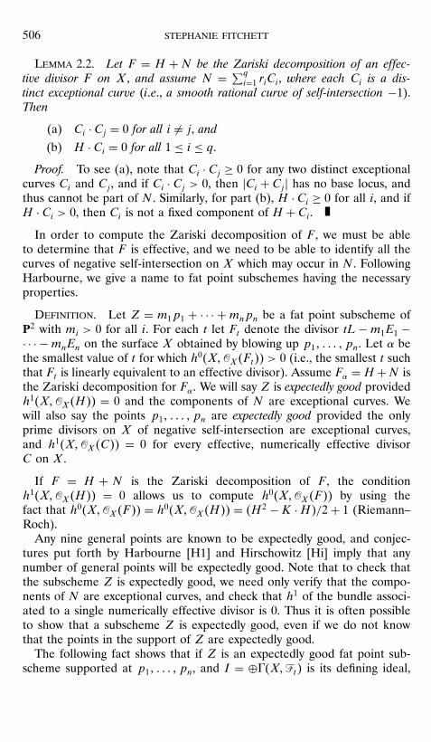
514 stephanie fitchett
and
�t = �X�tL−m1E1 − · · · −m11E11��where the mi’s are the multiplicities which appear in Z. The Zariski decom-position for �α = �1054 is
�α = �α ⊗ �⊗351 ⊗ �⊗20
2 ⊗ �⊗73︸ ︷︷ ︸
�α
�
where
�α = �X�33L− 13E1 − · · · − 13E6 − 5E7 − 4E8 − 4E9 − 4E10 − E11���1 = �X�23L− 9E1 − · · · − 9E6 − 4E7 − 3E8 − 3E9 − 3E10 − E11���2 = �X�8L− 4E1 − 3E2 − · · · − 3E6 − E7 − · · · − E10�� and
�3 = �X�8L− 3E1 − 4E2 − 3E3 − · · · − 3E6 − E7 − · · · − E10��It is not difficult to verify that � is the bundle associated to an effective,numerically effective divisor, h1�X��� = 0, and that each �i is a bundleassociated to an exceptional divisor. Hence Z is an expectedly good fatpoint subscheme. (One way to verify the claims is to apply Weyl transfor-mations to see that each divisor can be transformed to one which resideson a blow-up of eight or fewer points of P2, where a finite set of generatorsfor the numerically effective cone is known, as are the exceptional divisors.See [H1].)
The decomposition for �α yields the following decompositions for �α+1and �α+2:
�α+1 = � ⊗ �α ⊗ �⊗231 ⊗ �⊗8
2 ⊗ �⊗73︸ ︷︷ ︸
�α+1
⊗�⊗121 ⊗ �⊗12
2︸ ︷︷ ︸�α+1
�α+2 = � ⊗� ⊗ �α ⊗ �⊗351 ⊗ �⊗16
2 ⊗ �⊗73︸ ︷︷ ︸
�α+2
⊗ �⊗42︸︷︷︸
�α+2
�
We are now ready to examine νt for all t. Using Lemma 2.3 andRiemann–Roch we have
να = s��α−1� = h0�X��α� = 3�
να+1 = s��α� = s��α ⊗ �α�= s��α� + h0�X��α+1� − h0�X��α ⊗��= s��α� + 385− 38 = s��α� + 347�

generators for fat point ideals 515
The methods of this article do not allow determination of s��α�, butCampanella’s bounds [Cam] can be computed for s��α�. We show laterthat, for t > α+ 1, the bounds for νt developed here are always at least asgood as Campanella’s. Below, Campanella’s bounds for this example areshown for comparison purposes.Continuing, we have
να+2 = s��α+1� = s�� ⊗ � ⊗ � �= s��α+1 ⊗ �α+1�= s��α+1� + h0�X��α+2� − h0�X�� ⊗ �α+1�= s�� ⊗ �α ⊗ �⊗23
1 ⊗ �⊗82 ⊗ �⊗7
3 � + 1316− 1070
= s�� ⊗ �⊗231 ⊗ �⊗8
2 ⊗ �⊗73 � + 246�
By Theorem 3.3, we see that
120 = 3+ 9 · 13 ≤ s�� ⊗ �⊗231 � ≤ �4 · 5�/2 + 9 · 13 = 127
12 ≤ s�� ⊗ �⊗82 � ≤ 12� and
6 ≤ s�� ⊗ �⊗73 � ≤ 6�
By Lemma 2.5, s�� ⊗ �⊗231 ⊗ �⊗8
2 ⊗ �⊗73 � = s�� ⊗ �⊗23
1 � + s�� ⊗ �⊗82 � +
s�� ⊗ �⊗73 �, so
138 ≤ s�� ⊗ �⊗231 ⊗ �⊗8
2 ⊗ �⊗73 � ≤ 145�
This gives
384 ≤ να+2 ≤ 391�
Similarly, we find
να+3 = s��α+2�= s��α+2 ⊗ �α+2�= s��α+2� + h0�X��α+3� − h0�X�� ⊗ �α+2�= s�� ⊗ �α+1 ⊗ �⊗12
2 ⊗ �⊗82 � + 2368− 2342
= s�� ⊗ �⊗121 ⊗ �⊗8
2 � + 26�
and
12 ≤ s�� ⊗ �⊗121 ⊗ �⊗8
2 � ≤ 15�
which gives
38 ≤ να+3 ≤ 41�

516 stephanie fitchett
Finally,
να+4 = s��α+3� = s�� ⊗ �⊗42 � = 0�
and νt�I� = 0 for all t > α+ 4 by [DGM, Proposition 3.7].Summarizing, we have
vα = 3
να+1 = s��� + 347
384 ≤ να+2 ≤ 391
38 ≤ να+3 ≤ 41
να+4 = 0�
Comparison of Bounds
The theorem below is a restatement of Campanella’s bounds [Cam] inthe case that I is a fat point ideal on the projective plane. In the theorem,β = min�t � �t is numerically effective� and τ = min�t � h1�X��t� = 0�,where It = ��X��t�.Theorem 4.1. If I is a homogeneous ideal of fat points in the coordinate
ring of P2, then for t ≤ τ + 1,
νt ≤ dim It − 2 dim It−1 + dim It−2 − εt� where εt =0 if t ≤ α1 if α < t ≤ β2 if t > β,
and
νt ≥{max�0� dim It − 3 dim It−1 + 3 dim It−2 − dim It−3� if t �= βmax�1� dim It − 3 dim It−1 + 3 dim It−2 − dim It−3� if t = β.
Computing Campanella’s bounds for our example directly yields
να = 3
376 ≤ να+1 ≤ 378
170 ≤ να+2 ≤ 548
0 ≤ να+3 ≤ 108
0 ≤ να+4 ≤ 5�
Making use of Lemma 2.3, and applying Campanella’s bounds to thenumerically effective pieces (�α��α+1, and �α+2), gives better bounds, but

generators for fat point ideals 517
ones that are still far from those available via Theorem 3.3:
να = 3
376 ≤ να+1 ≤ 378
246 ≤ να+2 ≤ 449
15 ≤ να+3 ≤ 93
0 ≤ να+4 ≤ 5�
In fact, the bounds obtained via the theorems of Section 3 are always atleast as good as Campanella’s in degrees beyond α + 1. Before we provethis, we present a short lemma and a corollary which rephrase Campanella’sbounds.
Lemma 4.2. Let I be a fat point ideal supported at general pointsp1� � � � � pn of P2, and let X be the surface obtained by blowing up the points.If Iα corresponds to a line bundle on X of the form �⊗r , where � = �X�C�for an exceptional curve C and 2 ≤ r ≤ C · L, then Campanella’s upperbound for νβ+1�I� is r�r − 1�/2 − 1.
Proof. We use the facts that Iα = ��X��⊗r� and β = α + 1 to findanother expression for Campanella’s upper bound for νβ+1�I�. Letting d =L · C, we have
dim�Iβ+1� − 2 dim�Iβ� + dim�Iβ−1� − 2
= h0�X��⊗2 ⊗ C⊗r� − 2h0�X�� ⊗ C⊗r� − 1
= α+ 2 − h0�X�� ⊗ C⊗r�= rd + 1− �1+ 2rd − r2 + 3+ r�/2 = r�r − 1�/2 − 1�
Corollary 4.3. Let I be a fat point ideal supported at general pointsp1� � � � � pn of P2, and let X be the surface obtained by blowing up the points.If Iα corresponds to a line bundle on X which has a Zariski decomposition� ⊗ �⊗qi=1�⊗ri
i �, where each �i = �X�Ci� for a distinct exceptional curveCi, ri ≤ C · L, and � is the sheaf of a numerically effective divisor H withh1�X��� = 0, then Campanella’s upper bound for νβ+1�I� is
∑qi=1 ri�ri −
1�/2 − 1.
Proof. Let N = ∑si=1 riCi, let � = �X�N�, and let K be a canonical
divisor on X. We want to show that dim�Iβ+1� − 2 dim�Iβ� + dim�Iβ−1� −2 = ∑s
i=1 ri�ri − 1�/2 − 1. We have (note that H ·N = 0 since H · Ci = 0

518 stephanie fitchett
for all i by Lemma 2.2)
dim�Iβ+1� − 2 dim�Iβ� + dim�Iβ−1� − 2
= h0�X��⊗2 ⊗ � ⊗ � � − 2h0�X�� ⊗ � ⊗ � � + h0�X�� ⊗ � � − 2
= α+ 3− h0�X�� ⊗ � ⊗ � � + h0�X�� ⊗ � � − 2
= α+ 1− 12�6+ 2L ·H + 2L ·N +H2 −K ·H +N2 −K ·N�
+ h0�X���
= α+ 1−(h0�X��� + 2 + α+ N
2 −K ·N2
)+ h0�X���
= −N2 −K ·N
2− 1
=q∑i=1
ri�ri − 1�2
− 1�
We can now verify our claim.
Theorem 4.4. For every ideal defining an expectedly good fat point sub-scheme of P2, the bounds derived from Theorem 3.3 are at least as good asCampanella’s for all t > α+ 1.
Proof. We first show that if Iα corresponds to a bundle of the form �⊗r ,where � = �X�C� for an exceptional curve C and r ≤ L ·C, then the resultsof Theorem 3.3 are as good as Campanella’s bounds in degree β+ 1. SinceCampanella’s lower bound in degree β+ 1 is always 0 when α < β, there isnothing to show for lower bounds. We begin by showing the upper boundsof Theorem 3.3 are less than or equal to r�r − 1�/2 − 1.If 1 ≤ r ≤ u+ 1, both bounds of Theorem 3.3 are 0, so there is nothing
to prove.If u+ 1 < r ≤ U , then upper bound in Theorem 3.3 is
�r − u− 1��r − u�2
≤ �r − 2��r − 1�2
= r�r − 1�2
− r + 1 <r�r − 1�
2− 1�
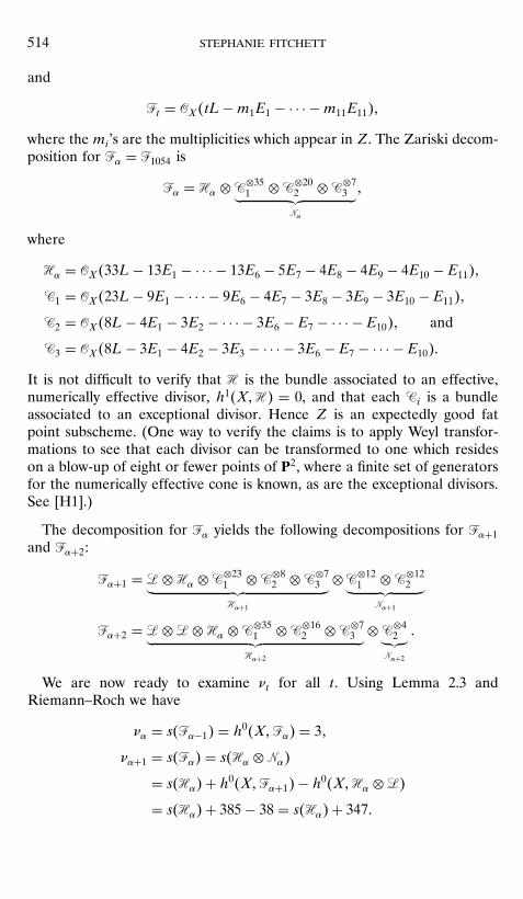
generators for fat point ideals 519
If r > U = u, we find
�r −U��r +U − d − 1� = �r − u��r − u− 1�
= �r − u�(r − d
2− 1
)
≤ �r − u�(r − r
2− 1
)
< �r − u� r2≤ �r − 1�r
2�
and because both ends are integers, �r −U��r +U − d − 1� ≤ r�r−1�2 − 1.
If r > U > u, we have
�U − u− 1��U − u�2
+ �r −U��r +U − d − 1�
= �U − u− 1��U − u�2
+ �r −U��r − u− 1�
<�r − u− 1��r −U + r − u�
2≤ �r − u− 1��u+ r − u�
2
≤ �r − u− 1�r2
≤ �r − 2�r2
≤ r�r − 1�2
− 1�
This completes the comparison of bounds for νβ+1 when Iα corresponds toa bundle of the form �⊗r .Next, consider the case that Iα corresponds to a line bundle of the form
⊗qi=1�⊗rii , with ri ≤ Ci · L, where �i = �X�Ci�. Since s�� ⊗ �⊗qi=1�⊗ri
i �� =∑si=1 s�� ⊗ �
⊗rii �, we see that the bounds obtained via Theorem 3.3 are
at least as good as Campanella’s since, if we compute the upper boundon s�� ⊗ �⊗qi=1�⊗ri
i �� by adding the upper bounds on each s�� ⊗ �⊗rii �,
the bound obtained via Theorem 3.3 is at least as good as Campanella’sbound for each term. Also, the sum of Campanella’s upper bounds for thes�� ⊗�
⊗rii �’s is at least as good as his bound for s�� ⊗ �⊗si=1�⊗ri
i ��, whichis∑si=1 ri�ri − 1�/2 − 1.
To see that the general case for t > α + 1 reduces to the case above,we note the following. As at the beginning of this section, we let �α =�α ⊗ �α be the Zariski decomposition for the line bundle �α associatedto Iα. Assume �α = ⊗qi=1�⊗ai
i , where each �i = �X�Ci� for an exceptionalcurve Ci. For t > α define �t−1, �t , and �t as follows:
�t−1 = ⊗qi=1�⊗min�L·Ci�−Nt−1·Ci�i
�t = � ⊗ �t−1 ⊗�t−1
�t = �t−1 ⊗�−1t−1�

520 stephanie fitchett
Then, for t > α+ 1, we have
νt�I� = s�� ⊗�t−2� + h0�X��t� − h0�X��t−1 ⊗���
But our bound for s�� ⊗�t−2� is at least as good as Campanella’s because,by construction, � ⊗�t−2 has the form � ⊗ �⊗qi=1�⊗ri
i � with ri ≤ L · Ci foreach i, which is the case shown above.
REFERENCES
[AH] J. Alexander and A. Hirschowitz, Polynomial interpolation in several variables, J.Algebraic Geom. 4 (1995), 201–222.
[Cam] G. Campanella, Standard bases of perfect homogeneous polynomial ideals of height2, J. Algebra 101 (1986), 47–60.
[Cat] M. V. Catalisano, “Fat” points on a conic, Comm. Algebra 19, No. 8 (1991), 2153–2168.
[CM1] C. Ciliberto and R. Miranda, Degenerations of planar linear systems, J. Reine Angew.Math. 501 (1998), 191–220.
[CM2] C. Ciliberto and R. Miranda, Linear systems of plane curves with base points ofequal multiplicity, Trans. Amer. Math. Soc., to appear.
[Cu] S. Cutkosky, Zariski decomposition of divisors on algebraic varieties, Duke Math. J.53 (1986), 149–156.
[DGM] E. D. Davis, A. V. Geramita, and P. Maroscia, Perfect homogeneous ideals: Dubreil’stheorems revisited, Bull. Sc. math. 108 (1984), 143–185.
[F1] S. Fitchett, “Generators of Fat Point Ideals on the Projective Plane,” Doctoral dis-sertation, University of Nebraska–Lincoln, 1997.
[F2] S. Fitchett, Maps of linear systems on blow-ups of the projective plane, J. Pure Appl.Algebra, to appear.
[FHH] S. Fitchett, B. Harbourne, and S. Holay, Resolutions of fat point ideals involving 8general points of P2� preprint, 2000.
[GGR] A. V. Geramita, D. Gregory, and L. Roberts, Monomial ideals and points in pro-jective space, J. Pure Appl. Algebra 40 (1986), 33–62.
[H1] B. Harbourne, The geometry of rational surfaces and Hilbert functions of points inthe plane, Canad. Math. Conf. proc. 6 (1986), 95–111.
[H2] B. Harbourne, Free resolutions of fat point ideals on P2, J. Pure Appl. Algebra 125(1998), 213–234.
[H3] B. Harbourne, The ideal generation problem for fat points, J. Pure Appl. Algebra145 (2000), 165–182.
[H4] B. Harbourne, An algorithm for fat point ideals on P2, Canad. J. Math. 52 (2000),123–140.
[H5] B. Harbourne, Anticanonical rational surfaces, Trans. Amer. Math. Soc. 349 (1997),1191–1208.
[Hi] A. Hirschowitz, Une conjecture pour la cohomologie des diviseurs sur les surfacesrationelles generiques, J. Reine Angew. Math. 397 (1989), 208–213.
[Ma] Y. I. Manin, “Cubic Forms,” North-Holland Mathematical Library 4, North-Holland, Amsterdam, 1986.
[Mi] R. Miranda, Linear systems of plane curves, Notices Amer. Math. Soc. 46 (1999),192–213.

generators for fat point ideals 521
[Mo] A. Moriwaki, Relative Zariski decomposition on higher dimensional algebraic vari-eties, Proc. Japan Acad. 62 (1986), 108–111.
[Mu] D. Mumford, Varieties defined by quadratic equations, in “Questions on AlgebraicVarieties, Corso C.I.M.E. 1969,” pp. 30–100, Cremoneses, Rome, 1969.
[N] M. Nagata, On rational surfaces, II, Mem. Coll. Sci. Univ. Kyoto Ser. A Math. 33(1960), 271–293.
[Z] O. Zariski, The theorem of Riemann–Roch for high multiples of an effective divisoron an algebraic surface, Ann. of Math. 76 (1962), 560–615.