On Bifurcations of Equilibria of Intrinsically Curved ...swigon/Papers/BCS_JElast.pdf · On Bifurcations of Equilibria of Intrinsically Curved, Electrically Charged, ... obtained

On Bifurcations of Equilibria of Intrinsically Curved,Electrically Charged, Rod-like Structures that ModelDNA Molecules in Solution

Yoav Y. Biton & Bernard D. Coleman & David Swigon

Received: 29 June 2006 /Accepted: 3 February 2007 /Published online: 30 May 2007# Springer Science + Business Media B.V. 2007

Abstract DNA molecules in the familiar Watson–Crick double helical B form can betreated as though they have rod-like structures obtained by stacking dominoes one on top ofanother with each rotated by approximately one-tenth of a full turn with respect to itsimmediate predecessor in the stack. These “dominoes” are called base pairs. A recentlydeveloped theory of sequence-dependent DNA elasticity (Coleman, Olson, & Swigon,J. Chem. Phys. 118:7127–7140, 2003) takes into account the observation that the step fromone base pair to the next can be one of several distinct types, each having its ownmechanical properties that depend on the nucleotide composition of the step. In the presentpaper, which is based on that theory, emphasis is placed on the fact that, as each base in abase pair is attached to the sugar-phosphate backbone chain of one of the two DNA strandsthat have come together to form the Watson–Crick structure, and each phosphate group in abackbone chain bears one electronic charge, two such charges are associated with each basepair, which implies that each base pair is subject to not only the elastic forces and momentsexerted on it by its neighboring base pairs but also to long range electrostatic forces that,because they are only partially screened out by positively charged counter ions, can renderthe molecule’s equilibrium configurations sensitive to changes in the concentration c of saltin the medium. When these electrostatic forces are taken into account, the equations ofmechanical equilibrium for a DNA molecule with N+1 base pairs are a system of μN non-linear equations, where μ, the number of kinematical variables describing the relativedisplacement and orientation of adjacent pairs is in general 6; it reduces to 3 when base-pairsteps are assumed to be inextensible and non-shearable. As a consequence of the long-range

J Elasticity (2007) 87:187–210DOI 10.1007/s10659-007-9103-7

Y. Y. Biton : B. D. Coleman (*)Department of Mechanics & Materials Science, Rutgers University,Piscataway, NJ 08854-8058, USAe-mail: [email protected], [email protected]

D. SwigonDepartment of Mathematics, University of Pittsburgh, Pittsburgh, PA 15260, USAe-mail: [email protected]

electrostatic interactions of base pairs, the μN×μN Jacobian matrix of the equations ofequilibrium is full. An efficient numerically stable computational scheme is here presentedfor solving those equations and determining the mechanical stability of the calculatedequilibrium configurations. That scheme is employed to compute and analyze bifurcationdiagrams in which c is the bifurcation parameter and to show that, for an intrinsicallycurved molecule, small changes in c can have a strong effect on stable equilibriumconfigurations. Cases are presented in which several stable configurations occur at a singlevalue of c.

Keywords Sequence dependent DNA elasticity . Electrically charged rod-like structures .

Bifurcation theory

Mathematics Subject Classifications (2000) 92-08 . 92D20 . 74K10 .

74B20 . 74G60 . 74G65

1 Introduction

For many purposes a molecule of duplex DNA can be treated as though it is a rod-likestructure that in a nanoscale drawing looks roughly like a stack of dominos (called basepairs) with each rotated approximately 36° relative to the one below it in the stack. A basepair is formed by joining together two nearly planar complementary nucleotide bases eachof which is attached to one of two sugar-phosphate chains. At the present time it appearsreasonable to assume that the elastic energy Ψ of a DNA configuration1 is the sum over n ofthe energy y n of interaction of the nth and (n+1)th base pairs and that y n is given by afunction of six numbers, called the kinematical variables (for the nth base pair step) thatdescribe the orientation and displacement of the (n+1)th base pair in the stack relative tothe nth. The values of these variables in the stress-free state and the function giving y n

depend on which nucleotide bases are in the nth and (n+1)th base pairs. Thus the geneticinformation in DNA determines not only the amino acid sequences of encoded proteins butalso the intrinsic geometry and deformability of DNA at the level of base-pair steps.

A naturally discrete theory of DNA elasticity that is based on the assumption thatΨ ¼P

n yn, with y n given by a function of six kinematical variables [1, 2], because it

takes into account the dependence of mechanical properties on nucleotide sequence, yieldsa model of DNA elasticity that is closer than the familiar continuum models to what wenow know about the structure and deformability of DNA.

Important to the present discussion is the fact that because each base in a base pair iscovalently bound to the sugar-phosphate backbone chain of one of the two DNA strandsthat form the Watson–Crick structure and each phosphate group bears one (negative)electronic charge, two such charges are associated with one base pair. The chargesassociated with two distinct base pairs exert on each other an electrostatic force ofrepulsion, the strength of which depends on the distance between them and theconcentration c of salt in the aqueous solution of DNA. The dependence on c resultsfrom the fact that salt ions of positive charge form clouds around the negatively charged

1We here use the term configuration as it is generally used in modern continuum mechanics and in the theoryof rods and structures. However, in discussions of such topics as protein structure and the chemical physicsof polymeric molecules, what we here call a “configuration” is often called a “conformation”.

188 Y.Y. Biton, et al.

sites on the DNA and in so doing partially screen out the electrostatic interaction of eachsite with others. As a consequence, an increase in c decreases the repulsion of nonadjacentbase pairs and weakens the tendency of electrostatic forces to straighten DNA molecules.Despite this partial screening, even under physiological conditions a DNA molecule issubject to intramolecular electrostatic forces that under appropriate circumstances (e.g.,when the molecule has intrinsic curvature) can cause equilibrium configurations to besensitive to the concentration of salt in the medium. As a consequence, DNA is not what incontemporary continuum mechanics is called “a simple material”, “a higher gradientmaterial”, or even a material with mechanical behavior that can be well approximated bythe behavior of such materials.

In the present essay we present a theory of the equilibrium configurations of electricallycharged and intrinsically curved rod-like structures that we believe serve as useful modelsof DNA molecules in aqueous solution. The theory goes beyond that of references [1] and[2] in that it renders explicit the nature and implications of electrostatic interactions betweennonadjacent base pairs. Both here and in those papers, the variational equations ofmechanical equilibrium for a DNA molecule with N+1 base pairs (bp) form a nonlinearsystem of μN equations for the μN unknown kinematical variables characterizing aconfiguration, where μ, the number of such variables at each base-pair step is, in general, 6but reduces to 3 when two neighboring base pairs are (or are assumed to be) much stifferfor changes in their relative displacement than for changes in their relative orientation.

When, as in [1] and [2], the electrostatic forces are not rendered explicit, is a system ofweakly coupled equations. Here, in marked contrast to those studies, because the force on abase pair depends on the position in space of all the other base pairs in the DNA molecule,the μN×μN Jacobian matrix for is full. The system here depends on the saltconcentration c, and the influence of c on the geometry and stability of equilibriumconfigurations is a matter of importance.

The mathematical assumptions of our theory are stated in Section 2. In Section 3 wepresent an efficient procedure for solving the system and determining the stability of theresulting equilibrium configurations. Toward the end of the paper, in Section 4, we applythat procedure to an example of a 450 bp DNA molecule that can be thought of as havingbeen formed by the end-to-end joining of three 150 bp DNA segments that are assumed tobe homogeneous and to have uniform curvature such that in an intrinsic (stress-free)configuration each would have the shape of a circular ring. That example illustrates thestrong influence that changes in the salt concentration c can have on the equilibriumconfigurations of intrinsically curved DNA and yields a bifurcation diagram with regions inwhich two very different, but yet both locally stable, equilibrium configurations occur at thesame value of c. In order to focus our attention on the role of electrostatic forces indetermining the properties of equilibrium configurations, for that example the DNAmolecule was deliberately chosen to be non-shearable and homogeneous in its mechanicalproperties.

2 Basic Assumptions and Governing Equations

As in [1] and [2] base pairs are represented here by rectangular objects, and the energy of aDNA molecule with N+1 base pairs (and hence N base-pair steps) is determined when thereis given, for n ¼ 1; . . . ;N þ 1, both the location x n of the center of the rectangle thatrepresents the nth base pair and a right-handed orthonormal triad dn1; d

n2; d

n3 that is

Electrical forces in DNA elasticity 189

embedded in the base pair as shown in Fig. 1.2 The polygonal curve composed of the Nline segments that connect the spatial points x1, x2,..., xN+1 is called the axial curve of themolecule. The elastic energy Ψ of a configuration is taken to be the sum over n of theenergy y n of interaction of the nth and (n+1)th base pairs, i.e.,

Ψ ¼XNn¼1

y n; ð2:1Þ

where y n, the elastic energy of the nth base-pair step, is given by a function of the relativeorientation and displacement of the (n+1)th base pair with respect to the nth, i.e., by afunction of the components (with respect to the basis dn1; d

n2; d

n3) of the vectors dnþ1j and

rn ¼ xnþ1 � xn. The components Dnij ¼ dni � dnþ1j of the vectors dnþ1j form a 3×3 orthogonal

matrix that is determined by three angles, qn1; qn2; q

n3, called the tilt, roll, and twist (see

Fig. 2). The displacement variables, rn1; rn2; r

n3, called shift, slide, and rise, are related to the

components rni ¼ rn � dni of rn by a coordinate transformation of the type

ρni ¼ ^ρi θn1; θ

n2; θ

n3; r

n1; r

n2; r

n3

� �; ð2:2Þ

which can be written in the form

rni ¼X3j¼1

bRji qn1; q

n2; q

n3

� �rnj : ð2:3Þ

2As seen in Fig. 1, the vectors dni are defined so that dn3 is perpendicular to with dn3 � xnþ1 � xnð Þ > 0;dn2 is parallel to the long edges of and points toward the short edge containing the corner ofthat is covalently bonded to the sugar-phosphate chain for which n increases in the 5′–3′ direction;dn1 ¼ dn2 � dn3 is parallel to the short edges of and points toward the major groove of the DNA. Adetailed discussion is given in [3].

Fig. 1 Schematic drawing of the nth base-pair step showing the vectors r n, dni , and dnþ1i . Each nucleotide base

in the nth base pair lies mainly on one side of the plane spanned by dn1 and dn3 and is covalently bonded at itsdarkened corner to one of the two sugar phosphate chains. The direction of that oriented chain is indicated by alight-face arrow; the chain itself is not shown. The gray-shaded long edges are in the minor groove of the DNA


The numbers Rnji ¼ bRji qn1; q

n2; q

n3

� �are the components of an orthogonal matrix, and the

functions ^ρi and bRji appearing are independent of n. The elastic energy y n of the nth base-pair step is thus given by a function eyn of six kinematical variables:

y n ¼ eyn qn1; qn2; q

n3; r

n1; r

n2; r

n3

� �: ð2:4Þ

The function eyn in the constitutive equation (2.4) depends on the nucleotide composition ofthe nth and (n+1)th base pairs. Unless one states otherwise, it is assumed that eyn, as afunction of qn1; q

n2; q

n3; r

n1; r

n2; r

n3

� �alone, is independent of the nucleotide composition of other

base pairs, e.g., the (n−1)th and (n+2)th, from which it follows that a base-pair step can beone of ten different types. However, our theory remains valid in more general cases in whichthe function eyn is assumed to be influenced by the composition of such other base pairs.

The kinematical variables qni and rni were introduced by Zhurkin et al. [4] and El Hassanand Calladine [5]. They are defined with precision in [5]. Properties of functions, such as^ρi, that relate r

ni and θ n

i to r ni and Dnij are discussed in detail in [1, 2, 5], and the Appendix in

this paper. The variables qni and rni are such that, for each fixed configuration of the DNAmolecule, a change in the choice of the direction of increasing n leaves θ2, θ3, ρ2, ρ3invariant but changes the sign of θ1 and ρ1.

3

We here consider a DNA molecule in an aqueous solution with a concentration c of amonovalent salt (e.g., NaCl). We assume that no external forces or moments act on a base pairother than those that result from the long range electrostatic interaction of negatively chargedphosphates in the same polymeric molecule. We further assume, as an approximation, that thetwo negative charges associated with each base pair are located at the barycenter of that basepair which implies that the electrostatic energy of a configuration has the form,

6 ¼ 1

2

XNþ1n¼1

8n; 8n ¼ e8n x1; . . . ; xNþ1� �

; ð2:5Þ

Fig. 2 Schematic representations of the kinematical variables that describe the relative orientation and displacementof consecutive base pairs: θ1 and θ2 are angles of rotation about two perpendicular lines that lie in the midplanebetween the base pairs; θ3 is an angle of rotation about a line l perpendicular to the midplane; ρ1 and ρ2 aremutually perpendicular displacements in directions parallel to the midplane; and ρ3 is a displacement along l. Eachdrawing illustrates one of the kinematical variables for the (artificial) case in which that variable has a positivevalue and the others (with the exception of ρ3) are set equal to zero

3General implications of this remark for the functions eyn are given in [1]. See also the remark madebelow after equation (2.21).


(in which 8n is the electrostatic energy associated with the nth base pair) and hence that basepairs do not sustain moments of electrostatic origin. In the present theory we employManning’s theory of charge condensation, which, as discussed in the paragraph containingequation (2.23), is in accord with euqation (2.5).

A configuration of the DNA molecule is said to be in equilibrium if the first variation ofthe total energy,

U ¼ Ψþ Φ; ð2:6Þvanishes for all variations that are compatible with the constraints imposed on the molecule.

Equation (2.5) and the theory developed in reference [1] here yield equations ofequilibrium that can be written in the form,

f n � f n�1 þ gn ¼ 0; mn �mn�1 þ rn � f n ¼ 0; n ¼ 1; 2; . . . ;N : ð2:7ÞFor n=1,2,..., N, f n and mn are the (non-electrostatic) force and moment that the (n+1)thbase pair exerts on the nth. The vectors −f 0 and −m0 equal the force and moment that theexternal world exerts on the base pair for which n=1; when the DNA molecule is assumedfree of such external forces and moments,

f 0 ¼ 0; m0 ¼ 0; gNþ1 � f N ¼ 0; mN ¼ 0: ð2:8ÞIn (2.7) and (2.8), gn equals the total electrostatic force exerted on the nth base pair by otherbase pairs in the same molecule and is given by the equation

gn ¼Xm 6¼n

Gmn ¼ � @6

@xn: ð2:9Þ

Here Gmn ¼ �Gnm is the electrostatic force (of repulsion) that the mth base pair exerts on thenth; that force is directed along the line connecting the barycenters of the two base pairs. Usingequation (2.9) one can show that the first two of the equations (2.8) together with the equationsof equilibrium (2.7) imply the third and the forth of the equations (2.8). In [1] it is shown that,for n=1,2,..., N, the components f ni and mn

i of f n and mn with respect to the local basisdn1; d

n2; d

n3 are

f ni ¼

X3j¼1

@eyn

@ρnj

@^ρj

@rni; f ni ¼ f n � dni ; ð2:10Þ

mni ¼

X3j¼1

*nij

@eyn

@θnjþX3k¼1

@eyn

@ρnk

@^ρk

@θnj

" #; mn

i ¼ mn � dni ; ð2:11Þ

where *nij ¼ b*ij θ

n1; θ

n2; θ

n3

� �with b*ij a function independent of n whose form is known.4

4See equations (A.1–A.5), (2.12–2.15) of [1], or the Appendix to this paper.


The equations (2.7), when taken together with (2.8–2.11), form a system of 6N equationsfor the 6N scalar variables qn1; q

n2; q

n3; r

n1; r

n2; r

n3, n=1,2,..., N. In the remainder of this paper

we emphasize the limiting case in which the DNA molecule is stiff with respect to (i.e.,strongly resistant to changes in) the kinematical quantities rn1; r

n2; r

n3 that characterize shift,

slide, and rise. That limit is one in which the displacement parameters rn1; rn2; r

n3 are

preassigned constants. In the limit, f n, like the pressure p in an incompressible fluid, is nolonger given by a local constitutive relation such as (2.10), but instead is determined by abalance law and boundary conditions. Here the appropriate balance law is the first equationof (2.7); the appropriate boundary conditions (here called end conditions) are the first andthird equations of (2.8); these relations yield the expression,

f n ¼ �Xnm¼1

gm; ð2:12Þ

that, by (2.9) and (2.5), relates f n to the axial curve and hence to the vector

Θ ¼ θ11; θ12; θ

13; θ

21; . . . ; θ

N3

� � ð2:13Þ

in IR3N. In the same limit, the term @eyn.@ρnk

� �@

^ρk.@θnj

� �in (2.11) loses meaning, and

we have

mni ¼

X3j¼1

* nij

@eyn

@θnj�X3k¼1

X3l¼1

f nl@bRlk

@θnjρnk

" #: ð2:14Þ

Here, as in (2.10) and (2.11), f ni ¼ f n � dni and mni ¼ mn � dni . When, as in the present case,

the numbers r11; r12; r

13; r

21; . . . ; r

N3 are preassigned, it follows from the relations

rni ¼ rn � d ni ; xn ¼ x1 þ

Xn�1p¼1

r p; ð2:15Þ

the equation (2.3), and expressions given in the Appendix for the dependence of Dnij ¼

dni � dnþ1j on qn1; qn2; q

n3 that, if Θ is known, then, to within an arbitrary rigid body rotation

and translation, the vectors d11; d12; d

13; d

21; . . . ; d

Nþ13 and the points x1, x2,..., xN+1 are also

known, and hence we may refer to Θ as the configuration of the molecule.Let us now concentrate our attention on equilibrium configurations, i.e., on solutions

q11; q12; q

13; q

21; . . . ; q

N3

� �of the equations (2.7) and (2.8) in which gn, f n, and mn are given by

(2.9), (2.12), and (2.14). An equilibrium configuration of a molecule obeying thesehypotheses will here be called stable if the 3N×3N square matrix A with the components,

A i;nð Þ j;mð Þ ¼ @2

@θni @θmj

U θ11; θ12; θ

13; θ

21; . . . ; θ

N3

� �; i; j ¼ 1; 2; 3; n;m ¼ 1; . . . ;N ; ð2:16Þ

is positive definite, i.e., if the second variation of the total energy,

δ2U ¼X

i¼1;2;3n¼1;...;N

Xj¼1;2;3m¼1;...;N

A i;nð Þ j;mð Þδθni δθ

mj ; ð2:17Þ


is (strictly) positive for every non-zero variation

δΘ ¼ δθ11; δθ12; δθ

13; δθ

21; . . . ; δθ

N3

� � ð2:18Þ

of configuration. We are particularly interested in the way the shape and stability ofequilibrium configurations depend on the salt concentration c.

We pause a moment to comment on our proposed criterion for stability. In applicationsof the present theory, equilibrium configurations of curved DNA molecules that are stablein the classical sense, but yet have symmetries implying the existence of variations withneutral directions, are rare. When they do occur, their presence is expected to be detectableso that such (neutral) variations are excluded when applying our criterion.

When r11; r12; r

13; r

21; . . . ; r

N3 are preassigned constants, the elastic energy associated with

the nth base-pair step is given by a function byn of the three kinematical variables qn1; qn2; q

n3:

yn ¼ byn θn1; θn2; θ

n3

� �: ð2:19Þ

For the calculations to be reported here we make the additional assumption that thisfunction is a quadratic form in the excess tilt $qn1, the excess roll $q

n2, and the excess twist

$qn3, which quantities are defined so that

θni ¼ oθni þ $θni ; ð2:20Þ

where the oqni are intrinsic values, i.e., values appropriate to a stress-free state of the nthbase pair step. Thus

yn ¼ 1

2

X3i¼1

X3j¼1

Fnij$θ

ni $θ

nj ; ð2:21Þ

where the moduli Fnij ¼ Fn

ji like the intrinsic parameters oqni are constants that depend on thenucleotide composition of the nth and (n+1)th base pairs. (Here, as is common practice, itis assumed that the elastic moduli and intrinsic parameters are independent of the nucleotidecomposition of other base pairs, but our general theory and computational schemes do notrequire such an assumption.)

One may think of Fn11 and Fn

22 as the (local) coefficients of rigidity for bending and ofFn33 as the corresponding coefficient for twisting. Quadratic energy functions of the form

(2.21) are approximations useful for small values of $θni .The observation made at the beginning of this section to the effect that a change in the

choice of the direction of increasing n leaves θ2 and θ3 invariant but changes the sign of θ1here places no á priori restriction on the modulus Fn

23 coupling roll to twist but does implythat the moduli that couple tilt to roll and tilt to twist obey the relations

Fn12 ¼ �F

N�nþ112 ; Fn

13 ¼ �F N�nþ1

13 ; ð2:22Þ

where F N�nþ1

12 and F N�nþ1

13 are moduli associated with a base-pair step that iscomplementary to the nth step. (For example, if a step has on one strand the sequenceAG (or AT), then for its complementary step the corresponding sequence is CT (or AT)). Itfollows that if the nth step is self-complementary, i.e., has the sequence AT, TA, GC, or CG,then (as discussed in [1]) Fn

12 ¼ 0, Fn13 ¼ 0.

For calculations of electrostatic interactions we here employ a form of Manning’s theoryof charge condensation [6] and obtain the following expression for the energy resulting


from the electrostatic interaction between the charge associated with the nth base pair andthe charges associated with other base pairs:5

8n ¼ QXm 6¼n

m 6¼n�1

e�kxnm

xnm; xnm ¼ xj n�xmj: ð2:23Þ

When measured in units of Å−1, the Debye screening parameter κ is given by the formula

k ¼ 0:329ffiffifficp

; ð2:24Þwhere c is the concentration of (monovalent) salt in moles per liter. For the constant Q wehave

Q ¼ q2�4πe0ew; ð2:25Þ

with e0 the permittivity of free space and ew the dielectric constant of water, and, in accordwith Manning’s theory [6, 8], q is set equal to 24% of the charge of the two phosphategroups associated with each base pair, i.e., q ¼ 2� 0:24e�, where e− is the charge of anelectron. For each n the summation in (2.23) is taken over all m from 1 to N+1 thatcorrespond to base pairs that are not adjacent to, or the same as, the nth base pair. Nearestneighbors are omitted from that summation because we take the position that the localelastic energy functions eyn�1 and eyn account for all interactions (including those ofelectrostatic origin) between the nth base pair and the two that are adjacent to it. When weinsert (2.23) into (2.5) and make use of (2.9), we obtain for the vector gn the relation

gn ¼ QXm 6¼n

m 6¼n�1

e�kxnm

xnm1

xnmþ k

� xn � xm

xnm: ð2:26Þ

Because knowledge of the 3N-dimensional vector Θ determines the vectors x n (see thesentence containing equation (2.15)), this last equation tells us that g n is given by a functionof Θ (which, albeit complicated, can be rendered explicit), and, by (2.12) and (2.14), soalso are the vectors f n and mn.

When we write equation (2.12) we are assuming that the force vectors f n obey the firstof the equilibrium equations (2.7) and the end condition f 0=0, which relations then yieldthe third of the equations (2.8). We obtain an equilibrium configuration when we find a3N-dimensional vector Θ that obeys the second of the equations (2.7) with mn as in (2.14)and f n as in (2.12).

To cast the second of the equations (2.7) into a form convenient for calculations, let usnow write mn

i , fni , r

ni for the components of mn, f n, r n with respect to the basis d11; d

12; d

13.

These components are related to the components of the same vectors with respect to thebasis d n

1 ; dn2 ; d

n3 through equations of the form,

mni ¼ d1i �mn ¼

X3j¼1

d1i � dnj� �

mnj ; ð2:27Þ

5See also the discussion of Westcott et al. [7].


etc., and hence depend on Θ. In this notation, the second of the equations (2.7) becomes

W Θð Þ ¼ 0; i:e:; wni Θð Þ ¼ 0; i ¼ 1; 2; 3; n ¼ 1; 2; . . . ;N ; ð2:28Þ

where

W ¼ w11;w

12;w

13;w

21; . . . ;w

N3

� �; ð2:29Þ

with

wni ¼ mn

i � mn�1i þ

X3j¼1

X3k¼1

rnj fnkeijk ; ð2:30Þ

and eijk is the permutation symbol. We are particularly interested in bifurcation diagrams forthe dependence of the solutions of equation (2.28) on the salt concentration c. The pro-cedure by which we numerically solve the 3N equations (2.28) and determine the stabilityof the equilibrium configurations so obtained is described below.

Remark When we wrote the equation (2.5) which, because we employ Manning’s chargecondensation theory, yields the equations (2.23–2.26), we made an approximation that willbe noticed by readers familiar with current ideas about DNA structure and base-pair levelmodels of DNA elasticity. We assumed “that the two negative charges associated with eachbase pair are located at the barycenter of that base pair.” In fact, those negative chargesbelong to the phosphate groups of two sugar phosphate chains that are at the surface of theDNA double helix and not at its center. However, Manning’s theory gives us reason forexpecting that the condensed counter ions (which, in the case of DNA in an aqueoussolution of monovalent salt, neutralize 76% of the charged phosphate groups) are notactually bound to the DNA macromolecule, i.e., are not localized at definite sites on thatmolecule, but are instead free to move in and out (and also along the axis) of a tube that hasa diameter that depends on c but exceeds the 20 Å steric diameter of the macromolecule.When one accepts the idea that the net effective charge of the DNA macromolecule is not tobe thought of as arising from charges at preassigned points but rather as the result of rapidfluctuations in a region interior to a tube of specified radius, it appears reasonable tosuppose that the assumption stated in quotes above does not introduce serious errors.

3 Computational Procedure

To solve the system of equations (2.28) when there is available a configuration *Θ that isclose to an equilibrium configuration Θ for the salt concentration c (for example, when onealready has found an equilibrium configuration for a salt concentration *c close to c), we

put b$Θ ¼ Θ � *Θ, b$Θ ¼ maxi;n

θni � *θni

�� and write6

0 ¼ W Θð Þ ¼ W �Θþ b$Θ� �¼ W �Θð Þ þ rW �Θð Þ b$Θh i

þ O b$Θ 2� ; ð3:1Þ

6We here use the symbol b$ in place of $ so that the components of b$Θ be distinguished from thequantities $qni in equations (2.20) and (2.21).


where rW �Θð Þ b$Θh iis linear in b$Θ, i.e., ∇W(*Θ) is the gradient of the function W(·)

evaluated at the configuration *Θ. This gradient is characterized by a 3N×3N square (but

not symmetric) matrix B with the components

B i;nð Þ j;mð Þ �Θð Þ ¼ @wni

@θmj�Θð Þ: ð3:2Þ

On omitting the terms O b$Q 2� one obtains the following system of 3N linear equations

for the 3N components θni � *θni of b$Θ:

wni �Θð Þ þ

Xj¼1;2;3m¼1;...;N

B i;nð Þ j;mð Þ �Θð Þ θmj � �θmj� �

¼ 0: ð3:3Þ

Although the matrix B is full and has entries that depend on the θ mj -derivatives of the

components gni , fni , and mn

i of gn, f n, and mn, we have been able to write a computer code

that collects the large number of algebraic terms in each functional component of W(·) andyields an analytical expression for each entry in B as a function of the (known) componentsof *Θ.7 Thus we avoid the need to employ numerical approximations for B, and we obtaina stable and efficient code for solving the linear system (3.3) as one step in a Newton–Raphson iterative procedure that yields solutions of the nonlinear system (2.28) to withinmachine accuracy.

Once we have in hand a procedure for calculating equilibrium configurations, we canturn to the matter of determining whether such a configuration is (locally) stable in thesense that for it the matrix A=A(Θ) of equations (2.16) and (2.17) is positive definite.Because the equations (2.7) and (2.8) are equivalent to the statement that the first variationδU of U vanishes for each variation in the vectors dni , i=1,2,3, n ¼ 1; . . . ;N þ 1, there is auseful algebraic relation between A and the matrix B characterizing the linearization ∇W(·)of the function W(·) of equations (2.28–2.30) that follows from the following formula [1]expressing variations dqni in the numbers qni in terms of variations in the vectors dni :

δθni ¼X3j¼1

*njid

nj � γnþ1 � γn

� �: ð3:4Þ

Here γn is the vector in the usual representation of the skew linear transformation, dnj 7!δdnj ,as an outer product, i.e.,

δdmj ¼ γm � dmj ; for j ¼ 1; 2; 3; ð3:5Þand *n

ji is as in (2.11). (More details are given in the Appendix.). If we put gni ¼ γn � d1i , wehave

δU ¼ �X

i¼1;2;3n¼1;...;Nþ1

wni Θð Þ gni ; ð3:6Þ

where wNþ1i ¼ mN

i . Equation (3.6) is equivalent to equation (3.20) of [1] and when com-bined with equations (2.28) and (2.30) yields

δ2U ¼ �X

j¼1;2;3m¼1;...;N

Xi¼1;2;3

n¼1;...;Nþ1

@wni

@θmjΘð Þδθmj gni : ð3:7Þ

7In view of (2.24), (2.26), (2.12), and (2.14), those expressions contain c as a parameter.


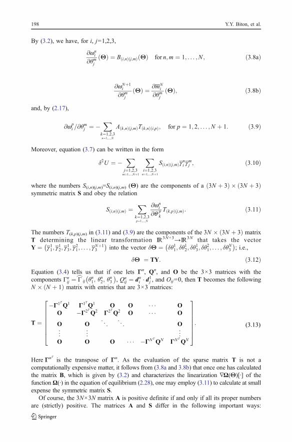
By (3.2), we have, for i, j=1,2,3,

@wni

@θmjΘð Þ ¼ B i;nð Þ j;mð Þ Θð Þ for n;m ¼ 1; . . . ;N ; ð3:8aÞ

@wNþ1i

@θmjΘð Þ ¼ @mN

i

@θmjΘð Þ; ð3:8bÞ

and, by (2.17),

@wpi =@θ

mj ¼ �

Xk¼1;2;3n¼1;...;N

A k;nð Þ j;mð ÞT k;nð Þ i;pð Þ; for p ¼ 1; 2; . . . ;N þ 1: ð3:9Þ

Moreover, equation (3.7) can be written in the form

δ2U ¼ �X

j¼1;2;3m¼1;...;Nþ1

Xi¼1;2;3n¼1;...;Nþ1

S i;nð Þ j;mð Þgni gmj ; ð3:10Þ

where the numbers S(i,n)(j,m)=S(i,n)(j,m) (Θ) are the components of a 3N þ 3ð Þ � 3N þ 3ð Þsymmetric matrix S and obey the relation

S i;nð Þ j;mð Þ ¼X

k¼1;2;3p¼1;...;N

@wni

@q pk

T k;pð Þ j;mð Þ: ð3:11Þ

The numbers T(k,p)(j,m) in (3.11) and (3.9) are the components of the 3N � 3N þ 3ð Þ matrixT determining the linear transformation IR3N+3→IR3N that takes the vectorY ¼ g11; g

12; g

13; g

21; . . . ; g

Nþ13

� �into the vector δΘ ¼ δθ11; δθ

12; δθ

13; δθ

21; . . . ; δθ

N3

� �; i.e.,

δΘ ¼ TY: ð3:12ÞEquation (3.4) tells us that if one lets Γn, Qn, and O be the 3×3 matrices with thecomponents *n

ij ¼ *_

ij θn1; θ

n2; θ

n3

� �, Qn

ij ¼ dni � d1j , and Oij=0, then T becomes the followingN � N þ 1ð Þ matrix with entries that are 3×3 matrices:

T ¼

�G1TQ1 G1TQ1 O O � � � OO �G2TQ2 G2TQ2 O � � � O

O O . .. . .

.O

..

. ... ..

.

O O O � � � �GNTQN GNT

QN

26666664

37777775:ð3:13Þ

Here ΓnT is the transpose of Γn. As the evaluation of the sparse matrix T is not acomputationally expensive matter, it follows from (3.8a and 3.8b) that once one has calculatedthe matrix B, which is given by (3.2) and characterizes the linearization ∇W(Θ)[·] of thefunction W(·) in the equation of equilibrium (2.28), one may employ (3.11) to calculate at smallexpense the symmetric matrix S.

Of course, the 3N×3N matrix A is positive definite if and only if all its proper numbersare (strictly) positive. The matrices A and S differ in the following important ways:

(3.13)


Whereas A characterizes the second variation of the energy U with respect to variations δΘin the vectorΘ in IR3N, which, because it describes (for each n) the orientation of the (n+1)thbase pair relative to the nth base pair, is invariant under rigid body motions of the DNAmolecule, the 3N þ 3ð Þ � 3N þ 3ð Þ matrix S characterizes the second variation of U withrespect to variations in the N+1 triads dn1; d

n2; d

n3

� �which are not invariant under rigid body

motions of the molecule. In a configurational perturbation that is no more than a rigid bodyrotation, the vector Y does not vanish, although the vector δΘ does. For the matrix A to bepositive definite it is necessary and sufficient that exactly 3 proper numbers of S be zero andall the other proper numbers of S be positive. Thus, when the 3N+3 proper numbers of S areplaced in a sequence (0, 0, 0, l1, l2,..., l3N) with l1≤l2≤ ...≤l3N, the equilibriumconfiguration under consideration is stable if and only if l1 is greater than zero.

In our study of the dependence of equilibrium configurations on salt concentration c, wecalculate and present bifurcation diagrams in which c is the bifurcation parameter and l1 theordinate. In such a diagram, an equilibrium configuration is stable when it corresponds to apoint above the abscissa.

We caution the reader that our stability criterion that all the proper numbers of A, or,equivalently, that all but 3 of the proper numbers of S, be positive, is correct only in casessuch as the present in which the DNA molecule is free of external loads and kinematicalconstraints and hence (2.8) holds. When the molecule is constrained so that Y has valuesonly in a (proper) subspace of IR3N+3 there will be an appropriate matrix other than S thatfurnishes a necessary and sufficient spectral criterion for stability.

4 An Example Illustrating Strong Dependence of Equilibrium Configurationson Salt Concentration

A DNA molecule with an axial curve that is not a closed curve will here be called open. Weconclude this essay with a presentation of computational results for an open molecule with450 base pairs (i.e., with N=449). We assume that the molecule is free of external forces andmoments and hence obeys (2.8). As we take the parameters rni , i=1,2,3 and n=1,...,N, to bepreassigned constants, we continue to employ the constitutive equation (2.21) for y n. In thepresent case the equations of equilibrium (2.28–2.30), with f n and mn as in (2.12) and (2.14),yield a system of 1,347 equations. Our computational procedure is described in Section 3.

So as to have an elementary example, we employ constitutive relations that havetransverse symmetry in the sense that: (1) for each n the shift and slide, rn1 and rn2, are bothzero and the rise rn3 has the standard value of 3.4 Å; (2) the moduli Fn

11 for tilt and Fn22 for

roll in equation (2.21) are equal, and there is no coupling between tilt, roll, and twist:

Fn11 ¼ Fn

22 ¼ constant; Fn12 ¼ Fn

13 ¼ Fn23 ¼ 0: ð4:1Þ

In the present case we put: Fn33

�Fn11 ¼ 1:05 and Fn

11 ¼ Fn22 ¼ 0:0427 kT=deg2.

We here make assumptions about the parameters oqni that are appropriate to a moleculeformed by ligating, end to end, three DNA segments, each containing 150 base pairs andeach having an intrinsic configuration in which it is circular in the sense that its axial curveis a perfect polygon of 150 sides. One way to obtain a model for such a molecule is toassume that it is homogeneous with, for each n, no intrinsic tilt, an intrinsic roll equal to2π/150 (i.e., 2.4°) and no intrinsic twist:

oθn1 ¼ oθ

n3 ¼ 0; oθ

n2 ¼ 2π=150: ð4:2Þ


Of course, in its common form (called B-DNA) a DNA molecule has a helical repeatlength close to 10 base pairs or, equivalently, values of oqn3 close to π/5, i.e., 36°. In thepresent case in which the molecule is transversely isotropic in the sense that (4.1) isassumed to hold, one can assign to the numbers oqni values that yield a molecule with

oθn3 � π=5 that has the same axial curve when stress-free and a mechanical behavior

identical to that of the molecule under consideration. This can be done by putting,8 for eachsubsegment with 10 base-pair steps, in addition to oθ

n3 � π=5,

oθk1 ¼

2π150

sinπ5

k � 1ð Þ þ π10

� �; oθ

k2 ¼

2π150

cosπ5

k � 1ð Þ þ π10

� �; ð4:3Þ

with, k = 1, . . . , 10. (From this point on, unless stated otherwise, angles are expressed inradians.)

The assumption (4.2) gives us an idealized model in which the molecule is homogeneousand planar in its intrinsic configuration. However, in reality oqn3 is not zero. A molecule obeying(4.3) would have oqn3 6¼ 0 and be planar in its intrinsic configuration, but it would also have oqn1and oqn2 strongly dependent on n and exhibiting both positive and negative values, which is notlikely to occur.9 On the other hand, a molecule that has oqn3 6¼ 0 and, in addition, has

oqn1; oqn2; oqn3 independent of n cannot have an intrinsic configuration that is even approxi-mately circular. For then, in the intrinsic configuration the two halves of each helical repeatlength would be bent in opposite directions. This is the reason why the 150 base pair minicirclestreated in reference [1] (and there called “DNA o-rings”) were taken to be composed of 15repetitions of a 10 base-pair segment in which 5 base-pairs constitute a homogeneousintrinsically straight subsegment and the remaining 5 constitute a homogeneous intrinsicallycurved subsegment in which the parameters oqn1; oqn2; oqn3 are adjusted so that when the 150base-pair molecule is closed (i.e., has its ends joined so that its axial curve is a closed curve) it isa stress-free ring. To be specific, the DNA o-rings treated in that paper had orn1; orn2; orn3

� � ¼0; 0; 3:4ð Þ for all n, but in each 10 base-pair unit, for the first 5 base pair steps,

oqn1; oq

n2; oq

n3

� � ¼ 0; 0; 36p180

� �; ð4:4aÞ

and, for the remaining 5,

oqn1; oq

n2; oq

n3

� � ¼ 0; 7:413p180

; 35:568p180

� �: ð4:4bÞ

It should be pointed out that DNA o-rings obtained in this way by joining straight segmentswith curved segments having oqn3 6¼ 0 and oqn1 ¼ 0 are nearly, but not perfectly, planar andhave a chiral structure (i.e., have axial curves that differ from their mirror images).10

The calculations we report in this paper were performed using the assumption (4.2) whichhere, as we stated above, is equivalent to the assumption (4.3). We have studied also cases inwhich (4.4a and 4.4b) hold and found that, when we make the “transverse symmetryassumptions” (1) and (2), the equilibrium configurations we calculate using (4.2) have axial

9Statistical analysis of X-ray structure data [17] indicates that, in general, oθ1 is approximately zero andoθ2 is not negative.10The writhe W of a closed curve [9–11] is a useful measure of the (total) chirality of the curve. For the axialcurve of a 150 base pair minicircle obeying (4.4a), (4.4b), W=0.078.

8This conclusion holds when one defines the variables θ n1 ; θ

n2 ; θ

n3 in accord with the procedure introduced in

[5] and discussed here in the Appendix. Properties of molecules obeying assumptions of the type (4.3) are

discussed in reference [16].


curves close to axial curves obtained using (4.4a and 4.4b).11 (The assumption (2) is vital tothe validity of this assertion.) Nevertheless, even under the assumptions (1) and (2), thebifurcation diagram implied by (4.2) has a topology that differs from that implied by (4.4a and4.4b). For a homogeneous molecule obeying (4.2), the system is perfect,12 and, inparticular, the branches issuing from an equilibrium configuration #Θ that is a bifurcationpoint can be found using a method in which one starts with a configuration Θ in aneighborhood of #Θ and searches for solutions of by successive adjustments of trialconfigurations generated by adding to #Θ vectors that are parallel to the characteristic vectorfor the proper number of S=[S(i, n)(j, m)] that vanishes at #Θ.13 (Here S(i,n)(j,m) is as in equations(3.10) and (3.11)). Both pitchfork and fold bifurcations are observed when (4.2) holds.

For a (periodic but not globally homogeneous) molecule obeying the equations (4.4a and4.4b), the system is imperfect, its equilibrium paths are not connected to each other, and thepitchfork bifurcations of the present system are replaced by folds each of which contains acritical point at which a proper number lq of S changes sign and a bifurcation-free equilibrium

Fig. 3 Four configurations on the primary branch H that are global minimizers of the total energy U at theindicated (monovalent) salt concentration c. The scale of length is the same for each case, and the lines ofview for the upper and lower drawings are perpendicular. c is expressed in moles per liter, U in units of kTwith T=300 K, and, because angles are here expressed in radians, 11, the smallest proper number of thematrix S, is expressed in units of 10−2kT

13In the present example, the characteristic space of S corresponding to a (vanishing) proper number lq isunidimensional. The search procedure just described can be generalized to cases in which proper numbers aredegenerate.

11The highly curved sequences found in the kinetoplast DNA of Trypanosmamatidae [12–15] more closelyresemble a periodic sequence obeying equations (4.4a and 4.4b) than a homogeneous sequence obeying(4.3).12In the sense in which the term is used in [18].


path is nearby. (Analogues in the theory of elasticity are discussed in the text of Thompson andHunt [18].) The observed behavior of the imperfect system obeying (4.4a and 4.4b) is theresult of (a) non-planarity and chirality of the axial curve in the stress-free configuration and(b) the fact that a DNA molecule containing an integral number of helical repeat units obeying(4.4a and 4.4b) has intrinsic directionality, because the 5 base-pair segment at one of its ends isintrinsically strait while that at the other end is intrinsically curved. In a paper now inpreparation we shall present detailed calculations illustrating the similarities and differencesbetween the behavior of a perfect system that obeys (4.2) and an imperfect system of thesame order (3N) that obeys the more realistic assumption (4.4a and 4.4b).

A DNA molecule is approximately a tube with a cross sectional diameter of 20 Å and isso represented in Fig. 3 and Figs. 5, 6, 7, 8, 9 and 10. In its intrinsic configuration, the 450base pair DNA molecule under consideration would have an axial curve with the form of atriply wound (planar) circle. Because the molecule cannot penetrate itself, that stress-freeconfiguration is not physically attainable. For values of c less than 1.2 M (1.2 molar) ourcalculations showed the existence of stable equilibrium configurations for which the axialcurve of the molecule is close to a helix with a pitch greater than 20 Å, and suchconfigurations, as they are free from self-penetration, are physically attainable. Theexamples in Fig. 3, for values of c in a range of interest to experimenters,14 lie on thebranch labeled H in the bifurcation diagram of Fig. 4. Each point on that branch

Fig. 4A Bifurcation diagram for equilibrium configurations presented as a graph of λ1, the smallest propernumber of the matrix S of equation (3.11), versus the salt concentration c. Configurations with λ1>0 are(locally) stable. Small circles denote configurations shown in Fig. 3 or Figs. 5, 6, 7, 8, 9 and 10. The(diamond) indicates a bifurcation point. The stem branch P and the primary branches H and Es are drawn inboldface, the secondary branches Eα and Eβ in lightface

14DNA denatures when c is less than 10−3 M.


corresponds to two solutions of (2.28) of equal energy but opposite chirality (theapproximating helix is right-handed for one and left-handed for the other, but in thepresent case are otherwise congruent). As branch H lies in a region where l1 is positive,each configuration on it is stable. Our careful and extensive calculations indicate that amuch stronger statement can be made: each configuration on branch H is not just a local butalso a global minimizer of the total energy U for the same value of c.

Fig. 4B Enlargement of the rectangular region that is bounded by dashed lines in Fig. 4A

Fig. 5 The planar configuration on the stem branch P with c ¼ 2� 10�4 M. This configuration is globallystable


Fig. 6 Two equilibrium configurations with c ¼ 5� 10�4 M. The planar configuration p#9 is unstable. (Thesharp symbol indicates lack of stability.) The configuration h9 is globally stable

Fig. 7 Four distinct equilibrium configurations with c ¼ 1:12� 10�2 M. The configurations es#5 and e!#5are unstable; e"5 is locally stable; h5 is globally stable


Branch H originates at a pitch fork bifurcation of a branch labeled P, each point of whichcorresponds to a single planar equilibrium configuration. At this bifurcation point c ¼c� ¼ 3:26� 10�4 M and l1=0. For c>c* each configuration in P is unstable; for c<c* theconfigurations in P are global minimizers of U. A stable configuration that lies on P wherec ¼ 2� 10�4 M is shown in Fig. 5. That configuration and the helical configurations

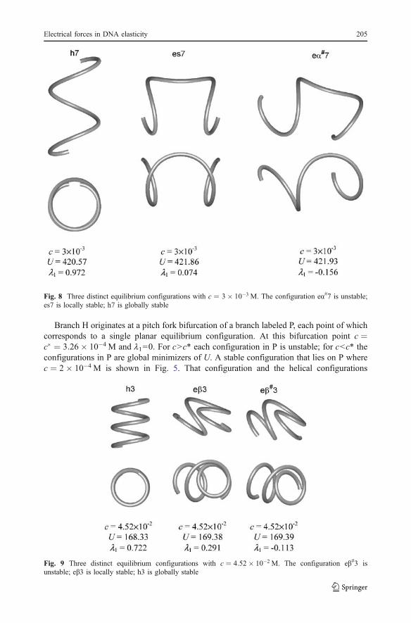
Fig. 8 Three distinct equilibrium configurations with c ¼ 3� 10�3 M. The configuration e!#7 is unstable;es7 is locally stable; h7 is globally stable

Fig. 9 Three distinct equilibrium configurations with c ¼ 4:52� 10�2 M. The configuration e"#3 isunstable; e"3 is locally stable; h3 is globally stable


shown in Fig. 3 illustrate the sensitivity of globally stable equilibrium configurations tochanges in salt concentration. In Fig. 6 one sees two equilibrium configurations at a valueof c close to but above c*, the configuration h9 is in H and the other, p#9, is in P. Theconfiguration h9 is chiral and globally stable but is not very well approximated by a helix.

The branch P may be considered a stem branch containing bifurcation points at whichprimary branches originate. As one moves along P in the direction of increasing c, oneencounters first the branch H and then a branch labeled Es that originates at a pitchforkbifurcation at which l2=0 and c ¼ 6:30� 10�4 M. The configurations on branch Es aresymmetric in the sense that their axial curves have a plane of symmetry. In the classical theoryof intrinsically helical rods, configurations that have been subjected to tensile loads and have,like those on branch Es, two approximately helical subregions of opposite handedness and aseparating transition region (see, e.g., the unstable configuration es#5 in Fig. 7, and the locallystable configuration es7 in Fig. 8) are occasionally called “perversions”.15 We here prefer to saythat the configurations es#5 and es7 are “everted helical configurations”.

Secondary branches labeled E! and E" originate at bifurcation points of the primarybranch Es with l1=0 and are comprised of configurations that are not symmetric. Two

Fig. 10 Three distinct equilibrium configurations with c=0.1 M, a value of c less than but very close to thecritical value c#=0.l0l M. The configuration e"#2 is unstable; e"2 is locally stable; h2 is globally stable

15Domokos and Healey [19], in a recent study of the theory of transversely isotropic, inextensible Kirchhoffrods of finite length with uniform nonzero intrinsic curvature and zero intrinsic torsion, developed a theoryappropriate to cases in which such a rod is subject to the following end conditions: the two ends are clampedso that their cross sections stay perpendicular to the line .: connecting their mid-points, neither end ispermitted to rotate about : , and the applied tensile force f acts along : . They find that, when the rod’sintrinsic curvature and the (positive) tension f are in appropriate ranges, the rod has stable configurations,called “perversions”, that are strikingly similar to the “everted helical configurations” found in ourinvestigation. (In an earlier investigation, Goriely and Tabor [20] found, in the context of periodicconfigurations for infinite rods, equilibrium solutions of the type just described for finite rods subject to endconditions.) We believe it interesting that these two types of results, with one obtained for curved rods free oflong range forces but subject to tensile loads at their ends, and the other for curved rodlike structures thathave free ends but bear internal electrostatic forces of repulsion, give rise to such closely similarconfigurations, although in one case the ends are free of applied forces and moments and in the other areclamped in such way that, at each end of a rod, the tangent to the rod axis is parallel to : .


examples, e!#5 and e"5, are shown in Fig. 7. (See also e!#7 in Fig. 8, e"#3, e"3 in Fig. 9,and e"#2, e"2 in Fig. 10.) The bifurcation diagram for the DNA molecule underconsideration has regions in which several distinct equilibrium configurations with morethan one of them stable occur at a single value of c. This is the case for c in the range ofvalues appropriate to Fig. 4a.16 Shown in Figs. 7, 8, and 9 are 4 equilibrium configurationsthat occur at c ¼ 1:12� 10�2 M, 3 at c ¼ 3� 10�3 M, and 3 at c ¼ 4:52� 10�2 M; ineach of these cases two of the distinct configurations are stable.17 In the small subrange1:41� 10�2M < c < 1:48� 10�2M of the range shown in Fig. 4b, i.e., for values of cbetween the first and second depicted folds on the branch E", there are 3 distinct stableconfigurations, with 2 on the branch E" and 1 on the branch H. For values of c greater thanc#=0.101 M (a critical value attained at the point on the third fold of the branch E" at whichl1=0), configurations in the branch H are the only stable configurations. Therefore a smallincrease in c from a value below c# to a value above c# will give rise to a transition from alocally stable configuration on the branch E" to a globally stable configuration on thebranch H.18 In Fig. 10 are shown 2 configurations on the branch E" and a configuration onthe branch H for c=0.1 M, a value that is very close to, but less than, c#.

Acknowledgements We thank Professor Gabor Domokos for useful discussions about the stability ofcomputational schemes for solving non-linear systems of equations related to those considered here. Thisresearch was supported by the National Science Foundation under Grants DMS-0514470 and DMS-0516646.

Appendix

In this appendix we first discuss El Hassan and Calladine’s procedure [5] for constructingtheir relation between the six kinematical variables qn1; q

n2; q

n3, r

n1; r

n2; r

n3 and the numbers

Dnij ¼ dni � dnþ1j and rni ¼ rn � dni ; we then give a derivation of the expression presented in

reference [1] for the quantities *nij ¼ b*ij θ

n1; θ

n2; θ

n3

� �appearing here in equations (2.11),

(2.14), and (3.13).Let dn1; d

n2; d

n3 and qn1; q

n2; q

n3 be given, and let the angles ξn and fn and a unit vector dnφ

(called the “hinge vector”), in the plane of dn1 and dn2, be defined by the relations:

ξn ¼ffiffiffiffiffiffiffiffiffiffiffiffiffiffiffiffiffiffiffiffiffiffiffiffiffiffiffiθn1� �2 þ θn2

� �2q; θn1 ¼ ξn sin φnð Þ; θn2 ¼ ξn cos φnð Þ; ðA:1Þ

dnφ ¼ �dn1 sinθn32� φn

� þ dn2 cos

θn32� φn

� : ðA:2Þ

18This critical value c# corresponds to an ionic strength not far from that occurring under physiologicalconditions.

17With the branch P a singular exception, the branches seen in Fig. 4 are generally sets of several branchesthat can be mapped into each other by energy preserving transformations of their constituent configurations.These transformations include that for which $θn1; $θ

n2; $θ

n3

� � 7! �$θn1; $θn2; �$θn3� �for each n (and hence

that changes only the chirality or “handedness” of the configuration) and that for which $θn1; $θn2;

�$θn3Þ7! �$θN�nþ11 ; $θN�nþ12 ; $θN�nþ13

� �for each n. In this paper when counting configurations we consider

two configurations the same if they are related by energy preserving transformations of these types. Forconfigurations on branches of order higher than 2 (which are not discussed in this paper), symmetry groupscharacterized by energy preserving transformations other than those generated by the two just described arerelevant.

16For each value of c for which there are stable and/or unstable configurations on branches seen in Fig. 4b,there is also a (stable) configuration that is on the branch H seen not in Fig. 4b but in Fig. 4a.


By applying to dn1; dn2; d

n3 a positive rotation about dnφ of magnitude ξn/2 one obtains an

orthonormal triad dnþa1 ; dnþa2 ; dnþa3 which one then rotates about dnþa3 through the angle

θn3�2 to obtain another orthonormal triad, d

nþ121 ; d

nþ122 ; d

nþ123 , which in reference [5] is called

the “mid-step triad.” (Of course, dnþ123 ¼ dnþα3 ). Here, as in [5], the displacement variables

rn1; rn2; r

n3 are, by definition, the components of rn with respect to the elements of the mid-

step triad:

ρni ¼ rn � dnþ12

i : ðA:3ÞThis last equation can be written in the form (2.3) with the numbers Rn

ij the components of

the vectors dnþ121 ; d

nþ122 ; d

nþ123 with respect to the basis dn1; d

n2; d

n3:

Rnij ¼ dni � d

nþ12j : ðA:4Þ

The procedure just described yields an explicit expression [5] for the function bRij in (2.3),namely,

Rnij ¼ bRij θ

n1; θ

n2; θ

n3

� � ¼X3k¼1

X3l¼1

Zikθn32� φn

� Ykl

ξn

2

� Zlj φ

nð Þ; ðA:5Þ

where Yij(ζ) and Zij(ζ) are, for each ζ, elements of the following rotation matrices:

Yij ζð Þ� ¼ cos ζð Þ 0 sin ζð Þ

0 1 0� sin ζð Þ 0 cos ζð Þ

24 35; Zij ζð Þ� ¼ cos ζð Þ � sin ζð Þ 0

sin ζð Þ cos ζð Þ 00 0 1

24 35: ðA:6Þ

The (fixed in space) hinge vector dnφ in equations (A.2) can be expressed in terms of itscomponents with respect to the mid-step triad as

dnφ ¼ dnþ121 sin φnð Þ þ d

nþ122 cos φnð Þ: ðA:7Þ

The triad dnþ11 ; dnþ12 ; dnþ13 can be obtained by applying to dnþ121 ; d

nþ122 ; d

nþ123 first a rotation

through an angle θn3�2 about d

nþ123 and then a rotation of magnitude ξ

n/2 about the hinge

vector dnφ. As the second rotation brings the original triad dnþ121 ; d

nþ122 ; d

nþ123 into coincidence

with dnþ11 ; dnþ12 ; dnþ13 , for the components of dnþ1j with respect to dnþ12i we have

dnþ12i � dnþ1j ¼

X3k¼1

X3l¼1

Zik �φnð ÞYkl ξn

2

� Zlj

θn32þ φn

� ; ðA:8Þ

and as

Dnij ¼ dni � dnþ1j ¼

X3k¼1

dni � dnþ12k

� dnþ12k � dnþ1j

� ; ðA:9Þ

in view of (A.4) and (A.8) we have [5],

Dnij ¼ bDij θ

n1; θ

n2; θ

n3

� � ¼X3k¼1

X3l¼1

Zikθn32� φn

� Ykl ξ

nð ÞZljθn32þ φn

� : ðA:10Þ


If we follow an argument given in [1] and note that each variation in the orthonormal triaddn1; d

n2; d

n3 is determined by a vector γn as shown in equations (3.5), i.e., δdni ¼ γn � dni , the

relations Dnij ¼ dni � dnþ1j will yield

X3j¼1

X3l¼1

Dnkj

@bDij

@θnlδθnl ¼

X3j¼1

ekijdnj � γnþ1 � γn

� �; ðA:11Þ

and if we make use of the fact that the matricesP3j¼1

Dnkj

@bDij

@θnlare skew, i.e., that

X3j¼1

Dnkj

@bDij

@qnl¼ �

X3j¼1

Dnij

@bDkj

@qnl; l ¼ 1; 2; 3; ðA:12Þ

we can write (A.11) in the formX3l¼1

Inilδθ

nl ¼ dni � γnþ1 � γn

� �; ðA:13Þ

where the components of the matrix Inil

� are

In1l ¼

X3j¼1

Dn2j

@bD3j

@θnl; In

2l ¼X3j¼1

Dn3j

@bD1j

@θnl; In

3l ¼X3j¼1

Dn1j

@bD2j

@θnl: ðA:14Þ

As was observed in [1] in a more general context, throughout the range of values of qn1; qn2; q

n3

appropriate to a DNA molecule, the matrix Inil

� with components In

il ¼ bIil θn1; θ

n2; θ

n3

� �is an

invertible matrix with inverse Inil

� �1, and hence one can solve equation (A.13) for dqnl to

obtain the relation (3.4) in which the numbers *nil ¼ *il θ

n1; θ

n2; θ

n3

� �are the components of the

transpose of Inil

� �1. It follows from the equations (A.6), (A.10), and (A.14) that

*nij ¼

� θn1ξn

sn þ θn2tn

2 tan ξn=2ð Þ � θn2ξn

sn � θn1tn

2 tan ξn=2ð Þ tan ξn=2ð Þtnθn1ξn t

nþ θn2sn

2 tan ξn=2ð Þθn2ξn t

n��θn1s

n

2 tan ξn=2ð Þ tan ξn=2ð Þsn

� θn2�2 θn1

�2 1

266664377775; ðA:15Þ

where

tn ¼ cosθn32� φn

� ; sn ¼ sin

θn32� φn

� : ðA:16Þ

The present equation (A.15) is the same as equation (A.1) of [1].

References

1. Coleman, B.D., Olson, W.K., Swigon, D.: Theory of sequence-dependent DNA elasticity. J. Chem. Phys.118, 7127–7140 (2003)

2. Olson, W.K., Swigon, D., Coleman, B.D.: Implications of the dependence of the elastic properties ofDNA on nucleotide sequence. Philos. Trans. R. Soc. Lond. A 362, 1403–1422 (2004)

3. Olson, W.K., Bansal, M., Burley, S.K., Dickerson, R.E., Gerstein, M., Harvey, S.C., Heinemann, U., Lu,X., Neidle, S., Shakked, Z., Wolberger, C., Berman, H.M.: A standard reference frame for the descriptionof nucleic acid base-pair geometry. J. Mol. Biol. 313, 229–237 (2001)


4. Zhurkin, V.B., Lysov, Y.P., Ivanov, V.: Anisotropic flexibility of DNA and the nucleosomal structure.Nucleic Acids Res. 6, 1081–1096 (1979)

5. El Hassan, M.A., Calladine, C.R.: The assessment of the geometry of dinucleotide steps in double-helicalDNA: A new local calculation scheme. J. Mol. Biol. 251, 648–664 (1995)

6. Manning, G.S.: Limiting laws and counterion condensation in polyelectrolyte solutions: I. Colligativeproperties. J. Chem. Phys. 51, 924–933 (1969)

7. Westcott, T.P., Tobias, I., Olson, W.K.: Modeling self-contact forces in the elastic theory of DNAsupercoiling. J. Chem. Phys. 107, 3967–3980 (1997)

8. Fenley, M.O., Manning, G.S., Olson, W.K.: Approach to the limit of counterion condensation.Biopolymers 30, 1191–1203 (1990)

9. White, J.H.: Self-linking and the Gauss integral in higher dimensions. Am. J. Math. 91, 693–728 (1969)10. Fuller, F.B.: The writhing number of a space curve. Proc. Natl. Acad. Sci. U. S. A. 68, 815–819 (1971)11. White, J.H.: Mathematical Methods for DNA Sequences. CRC, Boca Raton, Florida (1989)12. Marini, J.C., Levene, S.D., Crothers, D.M., Englund, P.T.: Bent helical structure in kinetoplast DNA.

Proc. Natl. Acad. Sci. USA 79, 7664–7668 (1982) (Correction ibid. 80, 7678 (1983))13. Diekmann, S., Wang, J.C.: On the sequence determinants and exibility of the kinetoplast DNA fragment

with abnormal gel electrophoretic mobilities. J. Mol. Biol. 186, 1–11 (1985)14. Haran, T.E., Kahn, J.D., Crothers, D.M.: Sequence elements responsible for DNA curvature. J. Mol.

Biol. 244, 135–144 (1994)15. Griffith, J., Bleyman, M., Rauch, C.A., Kitchin, P.A., Englund, P.T.: Visualization of the bent helix in

kinetoplast DNA by electron microscopy. Cell 46, 717–724 (1986)16. Calladine, C.R., Drew, H.R., Luisi, B.F., Travers, A.A.: Understanding DNA, 3rd edn. Elsevier, London

(2004)17. Olson, W.K., Gorin, A.A., Lu, X.-J., Hock, L.M., Zhurkin, V.B.: DNA sequence-dependent deformability

deduced from protein-DNA crystal complexes. Proc. Natl. Acad. Sci. U. S. A. 95, 11163–11168 (1998)18. Thompson, J.M.T., Hunt, G.W.: A General Theory of Elastic Stability. Wiley, London (1973)19. Domokos, G., Healey, T.J.: Multiple helical perversions of finite intrinsically curved rods. Int. J. Bifurc.

Chaos 15, 871–890 (2005)20. Goriely, A., Tabor, M.: The mechanics and dynamics of tendril perversion in climbing plants. Phys. Lett.

A. 250, 311–318 (1998)


Documents

On Bifurcations of Equilibria of Intrinsically Curved ...swigon/Papers/BCS_JElast.pdf · On Bifurcations of Equilibria of Intrinsically Curved, Electrically Charged, ... obtained