ON AUGMENTED LAGRANGIAN METHODS WITH ...martinez/abmstango.pdf(a) Minimize the Augmented Lagrangian on the appropriate “simple” set (Ω 2 in our case). (b) Update multipliers and

ON AUGMENTED LAGRANGIAN METHODS WITH GENERAL LOWER-LEVELCONSTRAINTS ∗

R. ANDREANI † , E. G. BIRGIN ‡ , J. M. MARTıNEZ § , AND M. L. SCHUVERDT ¶

Abstract. Augmented Lagrangian methods with general lower-level constraints are considered in the present research.These methods are useful when efficient algorithms exist for solving subproblems in which the constraints are only of thelower-level type. Inexact resolution of the lower-level constrained subproblems is considered. Global convergence is provedusing the Constant Positive Linear Dependence constraint qualification. Conditions for boundedness of the penalty param-eters are discussed. The reliability of the approach is tested by means of a comparison against Ipopt and Lancelot B.The resolution of location problems in which many constraints of the lower-level set are nonlinear is addressed, employingthe Spectral Projected Gradient method for solving the subproblems. Problems of this type with more than 3 × 106 vari-ables and 14 × 106 constraints are solved in this way, using moderate computer time. The codes are free for download inwww.ime.usp.br/∼egbirgin/tango/

Key words: Nonlinear programming, Augmented Lagrangian methods, global convergence, constraint qualifications, nu-merical experiments.

1. Introduction. Many practical optimization problems have the form

Minimize f(x) subject to x ∈ Ω1 ∩ Ω2,(1.1)

where the constraint set Ω2 is such that subproblems of type

Minimize F (x) subject to x ∈ Ω2(1.2)

are much easier than problems of type (1.1). By this we mean that there exist efficient algorithms forsolving (1.2) that cannot be applied to (1.1). In these cases it is natural to address the resolution of (1.1)by means of procedures that allow one to take advantage of methods that solve (1.2).

Let us mention here a few examples of this situation.• Minimizing a quadratic subject to a ball and linear constraints: This problem is useful in the

context of trust-region methods for minimization with linear constraints. In the low-dimensionalcase the problem may be efficiently reduced to the classical trust-region subproblem [38, 56],using a basis of the null-space of the linear constraints, but in the large-scale case this proceduremay be impractical. On the other hand, efficient methods for minimizing a quadratic within aball exist, even in the large-scale case [62, 65].• Bilevel problems with “additional” constraints [25]: A basic bilevel problem consists in mini-

mizing f(x, y) with the condition that y solves an optimization problem whose data depend onx. Efficient algorithms for this problem have already been developed (see [25] and referencestherein). When additional constraints (h(x, y) = 0, g(x, y) ≤ 0) are present the problem is morecomplicated. Thus, it is attractive to solve these problems using methods that deal with the dif-ficult constraints in an special way and solve iteratively subproblems with the easy constraints.

∗FIRST VERSION: OCTOBER 13, 2005†Department of Applied Mathematics, IMECC-UNICAMP, University of Campinas, CP 6065, 13081-970 Campinas SP,

Brazil. This author was supported by PRONEX-Optimization (PRONEX - CNPq / FAPERJ E-26 / 171.164/2003 - APQ1),FAPESP (Grant 01-04597-4) and CNPq. e-mail: [email protected]

‡ Department of Computer Science IME-USP, University of Sao Paulo, Rua do Matao 1010, Cidade Universitaria,05508-090, Sao Paulo SP, Brazil. This author was supported by PRONEX-Optimization (PRONEX - CNPq / FAPERJE-26 / 171.164/2003 - APQ1), FAPESP (Grants 01-04597-4 and 03-09169-6) and CNPq (Grant 300151/00-4). e-mail:[email protected]

§Department of Applied Mathematics, IMECC-UNICAMP, University of Campinas, CP 6065, 13081-970 Campinas SP,Brazil. This author was supported by PRONEX-Optimization (PRONEX - CNPq / FAPERJ E-26 / 171.164/2003 - APQ1),FAPESP (Grant 01-04597-4) and CNPq. e-mail: [email protected]

¶Department of Applied Mathematics, IMECC-UNICAMP, University of Campinas, CP 6065, 13081-970 Campinas SP,Brazil. This author was supported by PRONEX-Optimization (PRONEX - CNPq / FAPERJ E-26 / 171.164/2003 - APQ1)and FAPESP (Grants 01-04597-4 and 02-00832-1). e-mail: [email protected]

1

• Minimization with orthogonality constraints [32, 37, 58, 67]: Important problems on this classappear in many applications, such as the “ab initio” calculation of electronic structures. Rea-sonable algorithms for minimization with (only) orthogonality constraints exist, but they cannotbe used in the presence of additional constraints. When these additional constraints appear inan application the most obvious way to proceed is to incorporate them to the objective function,keeping the orthogonality constraints in the easy set Ω2.

• Control problems with algebraic constraints: Minimizing an objective function f(y, u) subjectto the discretization of y′ = f(y, u) is relatively simple using straightforward discrete controlmethodology. See [48, 53, 54] and references therein. The problem is more difficult if, in addi-tion, it involves algebraic constraints on the control or the state. These constraints are naturalcandidates to define the set Ω1, whereas the evolution equation should define Ω2.

• Problems in which Ω2 is convex but Ω1 is not: Sometimes it is possible to take profit of theconvexity of Ω2 in very efficient ways and we do not want to have this structure destroyed by itsintersection with Ω1.

These problems motivated us to revisit Augmented Lagrangian methods with arbitrary lower-levelconstraints. Penalty and Augmented Lagrangian algorithms seem to be the only methods that cantake advantage of the existence of efficient procedures for solving partially constrained subproblems ina natural way. For this reason, many practitioners in Chemistry, Physics, Economy and Engineeringrely on empirical penalty approaches when they incorporate additional constraints to models that weresatisfactorily solved by pre-existing algorithms.

The general structure of Augmented Lagrangian methods is well known [6, 23, 57]. An Outer Iterationconsists of two main steps:(a) Minimize the Augmented Lagrangian on the appropriate “simple” set (Ω2 in our case).(b) Update multipliers and penalty parameters.However, several decisions need to be taken in order to define a practical algorithm. For example, oneshould choose a suitable Augmented Lagrangian function. In this paper we use the Powell-Hestenes-Rockafellar PHR definition [46, 59, 63]. So, we pay the prize of having discontinuous second derivativesin the objective function of the subproblems when Ω1 involves inequalities. We decided to keep inequalityconstraints as they are, instead of replacing them by equality constraints plus bounds.

Moreover, we need a good criterion for deciding that a suitable approximate subproblem minimizerhas been found at Step (a). In particular, one must decide whether subproblem minimizers must befeasible with respect to Ω2 and which is the admissible level of infeasibility and lack of complementarityat these solutions. Bertsekas [5] analyzed an Augmented Lagrangian method for solving (1.1) in the casein which the subproblems are solved exactly.

Finally, simple and efficient rules for updating multipliers and penalty parameters must be given.Algorithmic decisions are taken looking at theoretical convergence properties and practical perfor-

mance. We are essentially interested in practical behavior but, since it is impossible to perform all thepossible tests, theoretical results play an important role in algorithmic design. However, only experiencetells one which theoretical results have practical importance and which do not. Although we recognizethat this point is controversial, we would like to make explicit here our own criteria:

1. External penalty methods have the property that, when one finds the global minimizers of thesubproblems, every limit point is a global minimizer of the original problem [33]. We think thatthis property must be preserved by the Augmented Lagrangian counterparts. This is the mainreason why, in our algorithm, we will force boundedness of the Lagrange multipliers estimates.

2. We aim feasibility of the limit points but, since this may be impossible (even an empty feasibleregion is not excluded) a “feasibility result” must say that limit points are stationary points forsome infeasibility measure. Some methods require that a constraint qualification holds at allthe (feasible or infeasible) iterates. In [15, 72] it was shown that, in such cases, convergence toinfeasible points that are not stationary for infeasibility may occur.

3. Feasible limit points must be stationary in some sense. This means that they must be KKTpoints or that a constraint qualification must fail to hold. The constraint qualification mustbe as weak as possible (which means that the optimality result must be as strong as possible).

2

Therefore, under the assumption that all the feasible points satisfy the constraint qualification,all the feasible limit points should be KKT.

4. Theoretically, it is impossible to prove that the whole sequence generated by a general Aug-mented Lagrangian method converges, because multiple solutions of the subproblems may existand solutions of the subproblems may oscillate. However, since one uses the solution of onesubproblem as initial point for solving the following one, the convergence of the whole sequencegenerally occurs. In this case, under stronger constraint qualifications, nonsingularity conditionsand the assumption that the true Lagrange multipliers satisfy the bounds given in the definitionof the algorithm, we must be able to prove that the penalty parameters remain bounded.

In other words, the method must have all the good global convergence properties of the ExternalPenalty method. In addition, when everything “goes well”, it must be free of the asymptotic instabilitycaused by large penalty parameters. It is important to emphasize that we deal with nonconvex problems,therefore the possibility of obtaining full global convergence properties based on proximal-point argumentsis out of question.

The algorithm presented in this paper satisfies those theoretical requirements. In particular, we willshow that, if a feasible limit point satisfies the Constant Positive Linear Dependence (CPLD) condition,then it is a KKT point. The CPLD condition was introduced by Qi and Wei [60]. In [3] it was provedthat CPLD is a constraint qualification, being weaker than the Linear Independence Constraint Qualifi-cation (LICQ) and than the Mangasarian-Fromovitz condition (MFCQ). A feasible point x of a nonlinearprogramming problem is said to satisfy CPLD if the existence of a nontrivial null linear combinationof gradients of active constraints with nonnegative coefficients corresponding to the inequalities impliesthat the gradients involved in that combination are linearly dependent for all z in a neighborhood of x.Since CPLD is weaker than (say) LICQ, theoretical results saying that if a limit point satisfies CPLDthen it satisfies KKT are stronger than theoretical results saying that if a limit point satisfies LICQ thenit satisfies KKT.

These theoretical results indicate what should be observed in practice. Namely:1. Although the solutions of subproblems are not guaranteed to be close to global minimizers, the

algorithm should exhibit a stronger tendency to converge to global minimizers than algorithmsbased on sequential quadratic programming.

2. The algorithm should find feasible points but, if it does not, it must find “putative minimizers”of the infeasibility.

3. When the algorithm converges to feasible points, these points must be approximate KKT pointsin the sense of [60]. The case of bounded Lagrange multipliers approximations corresponds to thecase in which the limit is KKT, whereas the case of very large Lagrange multiplier approximationsannounces limit points that do not satisfy CPLD.

4. Cases in which practical convergence occurs in a small number of iterations should coincide withthe cases in which the penalty parameters are bounded.

Our plan is to prove the convergence results and to show that, in practice, the method behaves asexpected. We will analyze two versions of the main algorithm: with only one penalty parameter and withone penalty parameter per constraint. For proving boundedness of the sequence of penalty parameterswe use the reduction to the equality-constraint case introduced in [5].

Most practical nonlinear programming methods published after 2001 rely on sequential quadraticprogramming (SQP), Newton-like or barrier approaches [1, 4, 14, 16, 19, 18, 35, 36, 39, 40, 51, 55, 66,70, 71, 73, 74, 75]. None of these methods can be easily adapted to the situation described by (1.1)-(1.2).We selected Ipopt, an algorithm by Wachter and Biegler available in the web [73] for our numericalcomparisons. In addition to Ipopt we performed numerical comparisons against Lancelot B [22].

The numerical experiments aim three following objectives:1. We will show that, in some very large scale location problems, to use a specific algorithm for

convex-constrained programming [10, 11, 12, 26] for solving the subproblems in the AugmentedLagrangian context is much more efficient than using general purpose methods like Ipopt andLancelot B.

2. Algencan is the particular implementation of the algorithm introduced in this paper for the3

case in which the lower-level set is a box. For solving the subproblems it uses the code Gencan[8]. We will show that Algencan tends to converge to global minimizers more often than Ipopt.

3. We will show that, for problems with many inequality constraints, Algencan is more efficientthan Ipopt and Lancelot B. Something similar happens with respect to Ipopt in problems inwhich the Hessian of the Lagrangian has a “not nicely sparse” factorization.

Finally, we will compare Algencan with Lancelot B and Ipopt using all the problems of the Cutercollection [13].

This paper is organized as follows. A high-level description of the main algorithm is given in Sec-tion 2. The rigorous definition of the method is in Section 3. Section 4 is devoted to global convergenceresults. In Section 5 we prove boundedness of the penalty parameters. In Section 6 we show the numericalexperiments. Applications, conclusions and lines for future research are discussed in Section 7.

Notation.We denote:

IR+ = t ∈ IR | t ≥ 0,

IR++ = t ∈ IR | t > 0,

IN = 0, 1, 2, . . .,

‖ · ‖ an arbitrary vector norm .

[v]i is the i−th component of the vector v. If there is no possibility of confusion we may also use thenotation vi.

For all y ∈ IRn, y+ = (max0, y1, . . . ,max0, yn).If F : IRn → IRm, F = (f1, . . . , fm), we denote ∇F (x) = (∇f1(x), . . . ,∇fm(x)) ∈ IRn×m.For all v ∈ IRn we denote Diag(v) ∈ IRn×n the diagonal matrix with entries [v]i.If K = k0, k1, k2, . . . ⊂ IN (kj+1 > kj∀j), we denote

limk∈K

xk = limj→∞

xkj.

2. Overview of the method. We will consider the following nonlinear programming problem:

Minimize f(x) subject to h1(x) = 0, g1(x) ≤ 0, h2(x) = 0, g2(x) ≤ 0,(2.1)

where f : IRn → IR, h1 : IRn → IRm1 , h2 : IRn → IRm2 , g1 : IRn → IRp1 , g2 : IRn → IRp2 . We assume thatall these functions admit continuous first derivatives on a sufficiently large and open domain. We defineΩ1 = x ∈ IRn | h1(x) = 0, g1(x) ≤ 0 and Ω2 = x ∈ IRn | h2(x) = 0, g2(x) ≤ 0.

For all x ∈ IRn, ρ > 0, λ ∈ IRm1 , µ ∈ IRp1+ we define the Augmented Lagrangian with respect to Ω1

[46, 59, 63] as:

L(x, λ, µ, ρ) = f(x) +ρ

2

m1∑i=1

([h1(x)]i +

λi

ρ

)2

+ρ

2

p1∑i=1

([g1(x)]i +

µi

ρ

)2

+

.(2.2)

The main algorithm defined in this paper will consist of a sequence of (approximate) minimizationsof L(x, λ, µ, ρ) subject to x ∈ Ω2, followed by the updating of λ, µ and ρ. A version of the algorithm withseveral penalty parameters may be found in [2]. Each approximate minimization of L will be called anOuter Iteration.

After each Outer Iteration one wishes some progress in terms of feasibility and complementarity. Theinfeasibility of x with respect to the equality constraint [h1(x)]i = 0 is naturally represented by |[h1(x)]i|.

4

The case of inequality constraints is more complicate because, besides feasibility, one expects to have a nullmultiplier estimate if gi(x) < 0. A suitable combined measure of infeasibility and non-complementaritywith respect to the constraint [g1(x)]i ≤ 0 comes from defining [σ(x, µ, ρ)]i = max[g1(x)]i,−µi/ρ. Sinceµi/ρ is always nonnegative, it turns out that [σ(x, µ, ρ)]i vanishes in two situations: (a) when [g1(x)]i = 0;and (b) when [g1(x)]i < 0 and µi = 0. So, roughly speaking, |[σ(x, µ, ρ)]i| measures infeasibility andcomplementarity with respect to the inequality constraint [g1(x)]i ≤ 0. If, between two consecutive outeriterations, enough progress is observed in terms of (at least one of) feasibility and complementarity, thepenalty parameter will not be updated. Otherwise, the penalty parameter is increased by a fixed factor.

The rules for updating the multipliers need some discussion. In principle, we adopt the classicalfirst-order correction rule [46, 59, 64] but, in addition, we impose that the multiplier estimates must bebounded. So, we will explicitly project the estimates on a compact box after each update. The reason forthis decision was already given in the introduction: we want to preserve the property of external penaltymethods that global minimizers of the original problem are obtained if each outer iteration computes aglobal minimizer of the subproblem. This property is maintained if the quotient of the square of eachmultiplier estimate over the penalty parameter tends to zero when the penalty parameter tends to infinity.We were not able to prove that this condition holds automatically for usual estimates and, in fact, weconjecture that it does not. Therefore, we decided to force the boundedness condition. The price paid bythis decision seems to be moderate: in the proof of the boundedness of penalty parameters we will need toassume that the true Lagrange multipliers are within the bounds imposed by the algorithm. Since “largeLagrange multipliers” is a symptom of “near-nonfulfillment” of the Mangasarian-Fromovitz constraintqualification, this assumption seems to be compatible with the remaining ones that are necessary toprove penalty boundedness.

3. Description of the Augmented Lagrangian algorithm. In this section we provide a de-tailed description of the main algorithm. Approximate solutions of the subproblems are defined as pointsthat satisfy the conditions (3.1)–(3.4) below. These formulae are relaxed KKT conditions of the problemof minimizing L subject to x ∈ Ω2. The first-order approximations of the multipliers are computed atStep 3. Lagrange multipliers estimates are denoted λk and µk whereas their safeguarded counterparts areλk and µk. At Step 4 we update the penalty parameters according to the progress in terms of feasibilityand complementarity.

Algorithm 3.1.Let x0 ∈ IRn be an arbitrary initial point. The given parameters for the execution of the algorithm are:

τ ∈ [0, 1), γ > 1, ρ1 > 0, −∞ < [λmin]i ≤ [λmax]i < ∞ ∀ i = 1, . . . ,m1, 0 ≤ [µmax]i < ∞ ∀ i = 1, . . . , p1,[λ1]i ∈ [[λmin]i, [λmax]i] ∀ i = 1, . . . ,m1, [µ1]i ∈ [0, [µmax]i] ∀ i = 1, . . . , p1. Finally, εk ⊂ IR+ is asequence of tolerance parameters such that limk→∞ εk = 0.Step 1. Initialization

Set k ← 1. For i = 1, . . . , p1, compute [σ0]i = max0, [g1(x0)]i.Step 2. Solving the subproblem

Compute (if possible) xk ∈ IRn such that there exist vk ∈ IRm2 , uk ∈ IRp2 satisfying

‖∇L(xk, λk, µk, ρk) +m2∑i=1

[vk]i∇[h2(xk)]i +p2∑

i=1

[uk]i∇[g2(xk)]i‖ ≤ εk,1,(3.1)

[uk]i ≥ 0 and [g2(xk)]i ≤ εk,2 for all i = 1, . . . , p2,(3.2)[g2(xk)]i < −εk,2 ⇒ [uk]i = 0 for all i = 1, . . . , p2,(3.3)

‖h2(xk)‖ ≤ εk,3,(3.4)

where εk,1, εk,2, εk,3 ≥ 0 are such that maxεk,1, εk,2, εk,3 ≤ εk. If it is not possible to find xk satisfying(3.1)–(3.4), stop the execution of the algorithm.Step 3. Estimate multipliers

For all i = 1, . . . ,m1, compute

[λk+1]i = [λk]i + ρk[h1(xk)]i,(3.5)5

[λk+1]i ∈ [[λmin]i, [λmax]i].(3.6)

(Usually, [λk+1]i will be the projection of [λk+1]i on the interval [[λmin]i, [λmax]i].) For all i = 1, . . . , p1,compute

[µk+1]i = max0, [µk]i + ρk[g1(xk)]i, [σk]i = max

[g1(xk)]i,−[µk]iρk

,(3.7)

[µk+1]i ∈ [0, [µmax]i].

(Usually, [µk+1]i = min[µk+1]i, [µmax]i.)Step 4. Update the penalty parameter

If max‖h1(xk)‖∞, ‖σk‖∞ ≤ τ max‖h1(xk−1)‖∞, ‖σk−1‖∞, then define ρk+1 = ρk. Else, defineρk+1 = γρk.Step 5. Begin a new outer iteration

Set k ← k + 1. Go to Step 2.

4. Global convergence. In this section we assume that the algorithm does not stop at Step 2. Inother words, it is always possible to find xk satisfying (3.1)-(3.4). Problem-dependent sufficient conditionsfor this assumption can be given in many cases.

We will also assume that at least a limit point of the sequence generated by Algorithm 3.1 exists. Asufficient condition for this is the existence of ε > 0 such that the set x ∈ IRn | g2(x) ≤ ε, ‖h2(x)‖ ≤ εis bounded. This condition may be enforced adding artificial simple constraints to the set Ω2.

Global convergence results that use the CPLD constraint qualification are stronger than previousresults for more specific problems: In particular, Conn, Gould and Toint [22] and Conn, Gould, Sartenaerand Toint [20] proved global convergence of Augmented Lagrangian methods for equality constraints andlinear constraints assuming linear independence of all the gradients of active constraints at the limitpoints. Their assumption is much stronger than our CPLD assumptions. On one hand, the CPLDassumption is weaker than LICQ (for example, CPLD always holds when the constraints are linear). Onthe other hand, our CPLD assumption involves only feasible points instead of all possible limit points ofthe algorithm.

Convergence proofs for Augmented Lagrangian methods with equalities and box constraints usingCPLD were given in [2].

We are going to investigate the status of the limit points of sequences generated by Algorithm 3.1.Firstly, we will prove a result on the feasibility properties of a limit point. Theorem 4.1 shows that, eithera limit point is feasible or, if the CPLD constraint qualification with respect to Ω2 holds, it is a KKTpoint of the sum of squares of upper-level infeasibilities.

Theorem 4.1. Let xk be a sequence generated by Algorithm 3.1. Let x∗ be a limit point of xk.Then, if the sequence of penalty parameters ρk is bounded, the limit point x∗ is feasible. Otherwise, atleast one of the following possibilities hold:

(i) x∗ is a KKT point of the problem

Minimize12

[ m1∑i=1

[h1(x)]2i +p1∑

i=1

max0, [g1(x)]i2]

subject to x ∈ Ω2.(4.1)

(ii) x∗ does not satisfy the CPLD constraint qualification associated with Ω2.Proof. Let K be an infinite subsequence in IN such that limk∈K xk = x∗. Since εk → 0, by (3.2) and

(3.4), we have that g2(x∗) ≤ 0 and h2(x∗) = 0. So, x∗ ∈ Ω2.Now, we consider two possibilities: (a) the sequence ρk is bounded; and (b) the sequence ρk is

unbounded. Let us analyze first Case (a). In this case, from some iteration on, the penalty parameters arenot updated. Therefore, limk→∞ ‖h1(xk)‖ = limk→∞ ‖σk‖ = 0. Thus, h1(x∗) = 0. Now, if [g1(x∗)]j > 0then [g1(xk)]j > c > 0 for k ∈ K large enough. This would contradict the fact that [σk]j → 0. Therefore,[g1(x∗)]i ≤ 0 ∀i = 1, . . . , p1.

6

Since x∗ ∈ Ω2, h1(x∗) = 0 and g1(x∗) ≤ 0, x∗ is feasible. Therefore, we proved the desired result inthe case that ρk is bounded.

Consider now Case (b). So, ρkk∈K is not bounded. By (2.2) and (3.1), we have:

∇f(xk) +∑m1

i=1([λk]i + ρk[h1(xk)]i)∇[h1(xk)]i +∑p1

i=1 max0, [µk]i

+ρk[g1(xk)]i∇[g1(xk)]i +∑m2

i=1[vk]i∇[h2(xk)]i +∑p2

j=1[uk]j∇[g2(xk)]j = δk,(4.2)

where, since εk → 0, limk∈K ‖δk‖ = 0.If [g2(x∗)]i < 0, there exists k1 ∈ IN such that [g2(xk)]i < −εk for all k ≥ k1, k ∈ K. Therefore, by

(3.3), [uk]i = 0 for all k ∈ K, k ≥ k1. Thus, by x∗ ∈ Ω2 and (4.2), for all k ∈ K, k ≥ k1 we have that

∇f(xk) +∑m1

i=1([λk]i + ρk[h1(xk)]i)∇[h1(xk)]i +∑p1

i=1 max0, [µk]i

+ρk[g1(xk)]i∇[g1(xk)]i +∑m2

i=1[vk]i∇[h2(xk)]i +∑

[g2(x∗)]j=0[uk]j∇[g2(xk)]j = δk.

Dividing by ρk we get:

∇f(xk)ρk

+∑m1

i=1

([λk]iρk

+ [h1(xk)]i

)∇[h1(xk)]i +

∑p1i=1 max

0, [µk]i

ρk+ [g1(xk)]i

∇[g1(xk)]i

+∑m2

i=1[vk]iρk∇[h2(xk)]i +

∑[g2(x∗)]j=0

[uk]jρk∇[g2(xk)]j = δk

ρk.

By Caratheodory’s Theorem of Cones (see [6], page 689) there exist Ik ⊂ 1, . . . ,m2, Jk ⊂ j | [g2(x∗)]j =0, [vk]i, i ∈ Ik and [uk]j ≥ 0, j ∈ Jk such that the vectors ∇[h2(xk)]ii∈Ik

∪ ∇[g2(xk)]jj∈Jkare

linearly independent and

∇f(xk)ρk

+∑m1

i=1

([λk]iρk

+ [h1(xk)]i

)∇[h1(xk)]i +

∑p1i=1 max

0, [µk]i

ρk+ [g1(xk)]i

∇[g1(xk)]i

+∑

i∈Ik[vk]i∇[h2(xk)]i +

∑j∈Jk

[uk]j∇[g2(xk)]j = δk

ρk.

(4.3)

Since there exist a finite number of possible sets Ik, Jk, there exists an infinite set of indices K1 suchthat K1 ⊂ k ∈ K | k ≥ k1, Ik = I , and

J = Jk ⊂ j | [g2(x∗)]j = 0(4.4)

for all k ∈ K1. Then, by (4.3), for all k ∈ K1 we have:

∇f(xk)ρk

+∑m1

i=1

([λk]iρk

+ [h1(xk)]i

)∇[h1(xk)]i +

∑p1i=1 max

0, [µk]i

ρk+ [g1(xk)]i

∇[g1(xk)]i

+∑

i∈I[vk]i∇[h2(xk)]i +

∑j∈J

[uk]j∇[g2(xk)]j = δk

ρk,

(4.5)

and the gradients

∇[h2(xk)]ii∈I∪ ∇[g2(xk)]jj∈J

are linearly independent.(4.6)

We consider, again, two cases: (1) the sequence ‖(vk, uk)‖, k ∈ K1 is bounded; and (2) the sequence‖(vk, uk)‖, k ∈ K1 is unbounded. If the sequence ‖(vk, uk)‖k∈K1 is bounded, and I ∪ J 6= ∅, thereexist (v, u), u ≥ 0 and an infinite set of indices K2 ⊂ K1 such that limk∈K2(vk, uk) = (v, u). Since ρkis unbounded, by the boundedness of λk and µk, lim[λk]i/ρk = 0 = lim[µk]j/ρk for all i, j. Therefore, byδk → 0, taking limits for k ∈ K2 in (4.5), we obtain:∑m1

i=1[h1(x∗)]i∇[h1(x∗)]i +∑p1

i=1 max0, [g1(x∗)]i∇[g1(x∗)]i

+∑

i∈Ivi∇[h2(x∗)]i +

∑j∈J

uj∇[g2(x∗)]j = 0.(4.7)

7

If I ∪ J = ∅ we obtain∑m1

i=1[h1(x∗)]i∇[h1(x∗)]i +∑p1

i=1 max0, [g1(x∗)]i∇[g1(x∗)]i = 0.Therefore, by x∗ ∈ Ω2 and (4.4), x∗ is a KKT point of (4.1).Finally, assume that ‖(vk, uk)‖k∈K1 is unbounded. Let K3 ⊂ K1 be such that limk∈K3 ‖(vk, uk)‖ =

∞ and (v, u) 6= 0, u ≥ 0 such that limk∈K3(vk,uk)

‖(vk,uk)‖= (v, u). Dividing both sides of (4.5) by ‖(vk, uk)‖ and

taking limits for k ∈ K3, we deduce that∑

i∈Ivi∇[h2(x∗)]i +

∑j∈J

uj∇[g2(x∗)]j = 0. But [g2(x∗)]j = 0

for all j ∈ J . Then, by (4.6), x∗ does not satisfy the CPLD constraint qualification associated with theset Ω2. This completes the proof.

Roughly speaking, Theorem 4.1 says that, if x∗ is not feasible, then (very likely) it is a local minimizerof the upper-level infeasibility, subject to lower-level feasibility. From the point of view of optimality, weare interested in the status of feasible limit points. In Theorem 4.2 we will prove that, under the CPLDconstraint qualification, feasible limit points are stationary (KKT) points of the original problem. SinceCPLD is strictly weaker than the Mangasarian-Fromovitz (MF) constraint qualification, it turns out thatthe following theorem is stronger than results where KKT conditions are proved under MF or regularityassumptions.

Theorem 4.2. Let xkk∈IN be a sequence generated by Algorithm 3.1. Assume that x∗ ∈ Ω1∩Ω2 isa limit point that satisfies the CPLD constraint qualification related to Ω1∩Ω2. Then, x∗ is a KKT pointof the original problem (2.1). Moreover, if x∗ satisfies the Mangasarian-Fromovitz constraint qualificationand xkk∈K is a subsequence that converges to x∗, the set

‖λk+1‖, ‖µk+1‖, ‖vk‖, ‖uk‖k∈K is bounded.(4.8)

Proof. For all k ∈ IN , by (3.1), (3.3), (3.5) and (3.7), there exist uk ∈ IRp2+ , δk ∈ IRn such that

‖δk‖ ≤ εk and

∇f(xk) +∑m1

i=1[λk+1]i∇[h1(xk)]i +∑p1

i=1[µk+1]i∇[g1(xk)]i

+∑m2

i=1[vk]i∇[h2(xk)]i +∑p2

j=1[uk]j∇[g2(xk)]j = δk.(4.9)

By (3.7), µk+1 ∈ IRp1+ for all k ∈ IN . Let K ⊂ IN be such that limk∈K xk = x∗. Suppose that [g2(x∗)]i < 0.

Then, there exists k1 ∈ IN such that ∀k ∈ K, k ≥ k1, [g2(xk)]i < −εk. Then, by (3.3), [uk]i = 0 ∀k ∈K, k ≥ k1.

Let us prove now that a similar property takes place when [g1(x∗)]i < 0. In this case, there existsk2 ≥ k1 such that [g1(xk)]i < c < 0 ∀k ∈ K, k ≥ k2.

We consider two cases: (1) ρk is unbounded; and (2) ρk is bounded. In the first case we havethat limk∈K ρk = ∞. Since [µk]i is bounded, there exists k3 ≥ k2 such that, for all k ∈ K, k ≥ k3,[µk]i + ρk[g1(xk)]i < 0. By the definition of µk+1 this implies that [µk+1]i = 0 ∀k ∈ K, k ≥ k3.

Consider now the case in which ρk is bounded. In this case, limk→∞[σk]i = 0. Therefore, since[g1(xk)]i < c < 0 for k ∈ K large enough, limk∈K [µk]i = 0. So, for k ∈ K large enough, [µk]i +ρk[g1(xk)]i < 0. By the definition of µk+1, there exists k4 ≥ k2 such that [µk+1]i = 0 for k ∈ K, k ≥ k4.

Therefore, there exists k5 ≥ maxk1, k3, k4 such that for all k ∈ K, k ≥ k5,

[[g1(x∗)]i < 0⇒ [µk+1]i = 0] and [[g2(x∗)]i < 0⇒ [uk]i = 0].(4.10)

(Observe that, up to now, we did not use the CPLD condition.) By (4.9) and (4.10), for all k ∈K, k ≥ k5, we have:

∇f(xk) +∑m1

i=1[λk+1]i∇[h1(xk)]i +∑

[g1(x∗)]i=0[µk+1]i∇[g1(xk)]i

+∑m2

i=1[vk]i∇[h2(xk)]i +∑

[g2(x∗)]j=0[uk]j∇[g2(xk)]j = δk,(4.11)

with µk+1 ∈ IRp1+ , uk ∈ IRp2

+ .8

By Caratheodory’s Theorem of Cones, for all k ∈ K, k ≥ k5, there exist

Ik ⊂ 1, . . . ,m1, Jk ⊂ j | [g1(x∗)]j = 0, Ik ⊂ 1, . . . ,m2, Jk ⊂ j | [g2(x∗)]j = 0,

[λk]i ∈ IR ∀i ∈ Ik, [µk]j ≥ 0 ∀j ∈ Jk, [vk]i ∈ IR ∀i ∈ Ik, [uk]j ≥ 0 ∀j ∈ Jk

such that the vectors

∇[h1(xk)]ii∈Ik∪ ∇[g1(xk)]ii∈Jk

∪ ∇[h2(xk)]ii∈Ik∪ ∇[g2(xk)]ii∈Jk

are linearly independent and

∇f(xk) +∑

i∈Ik[λk]i∇[h1(xk)]i +

∑i∈Jk

[µk]i∇[g1(xk)]i

+∑

i∈Ik[vk]i∇[h2(xk)]i +

∑j∈Jk

[uk]j∇[g2(xk)]j = δk.(4.12)

Since the number of possible sets of indices Ik, Jk, Ik, Jk is finite, there exists an infinite set K1 ⊂k ∈ K | k ≥ k5 such that Ik = I , Jk = J , Ik = I , Jk = J , for all k ∈ K1.

Then, by (4.12),

∇f(xk) +∑

i∈I[λk]i∇[h1(xk)]i +

∑i∈J

[µk]i∇[g1(xk)]i

+∑

i∈I [vk]i∇[h2(xk)]i +∑

j∈J [uk]j∇[g2(xk)]j = δk

(4.13)

and the vectors

∇[h1(xk)]ii∈I∪ ∇[g1(xk)]ii∈J

∪ ∇[h2(xk)]ii∈I ∪ ∇[g2(xk)]ii∈J(4.14)

are linearly independent for all k ∈ K1.If I ∪ J ∪ I ∪ J = ∅, by (4.13) and δk → 0 we obtain ∇f(x∗) = 0. Otherwise, let us define

Sk = maxmax|[λk]i|, i ∈ I,max[µk]i, i ∈ J,max|[vk]i|, i ∈ I,max[uk]i, i ∈ J.

We consider two possibilities: (a) Skk∈K1 has a bounded subsequence; and (b) limk∈K1 Sk = ∞. IfSkk∈K1 has a bounded subsequence, there exists K2 ⊂ K1 such that limk∈K2 [λk]i = λi, limk∈K2 [µk]i =µi ≥ 0, limk∈K2 [vk]i = vi, and limk∈K2 [uk]i = ui ≥ 0. By εk → 0 and ‖δk‖ ≤ εk, taking limits in (4.13)for k ∈ K2, we obtain:

∇f(x∗) +∑i∈I

λi∇[h1(x∗)]i +∑i∈J

µi∇[g1(x∗)]i +∑i∈I

vi∇[h2(x∗)]i +∑j∈J

uj∇[g2(x∗)]j = 0,

with µi ≥ 0, ui ≥ 0. Since x∗ ∈ Ω1 ∩ Ω2, we have that x∗ is a KKT point of (2.1).Suppose now that limk∈K2 Sk =∞. Dividing both sides of (4.13) by Sk we obtain:

∇f(xk)Sk

+∑

i∈I

[λk]iSk∇[h1(xk)]i +

∑i∈J

[µk]iSk∇[g1(xk)]i

+∑

i∈I[vk]iSk∇[h2(xk)]i +

∑j∈J

[uk]jSk∇[g2(xk)]j = δk

Sk,

(4.15)

where∣∣∣∣ [λk]i

Sk

∣∣∣∣ ≤ 1,

∣∣∣∣ [µk]iSk

∣∣∣∣ ≤ 1,

∣∣∣∣ [vk]iSk

∣∣∣∣ ≤ 1,

∣∣∣∣ [uk]jSk

∣∣∣∣ ≤ 1. Therefore, there exists K3 ⊂ K1 such that

limk∈K3[λk]iSk

= λi, limk∈K3[µk]iSk

= µi ≥ 0, limk∈K3[vk]iSk

= vi, limk∈K3[uk]jSk

= uj ≥ 0. Taking limitson both sides of (4.15) for k ∈ K3, we obtain:∑

i∈I

λi∇[h1(x∗)]i +∑i∈J

µi∇[g1(x∗)]i +∑i∈I

vi∇[h2(x∗)]i +∑j∈J

uj∇[g2(x∗)]j = 0.

9

But the modulus of at least one of the coefficients λi, µi, vi, ui is equal to 1. Then, by the CPLD condition,the gradients

∇[h1(x)]ii∈I∪ ∇[g1(x)]ii∈J

∪ ∇[h2(x)]ii∈I ∪ ∇[g2(x)]ii∈J

must be linearly dependent in a neighborhood of x∗. This contradicts (4.14). Therefore, the main partof the theorem is proved.

Finally, let us prove that the property (4.8) holds if x∗ satisfies the Mangasarian-Fromovitz constraintqualification. Let us define

Bk = max‖λk+1‖∞, ‖µk+1‖∞, ‖vk‖∞, ‖uk‖∞k∈K .

If (4.8) is not true, we have that limk∈K Bk = ∞. In this case, dividing both sides of (4.11) by Bk

and taking limits for an appropriate subsequence, we obtain that x∗ does not satisfy the Mangasarian-Fromovitz constraint qualification.

5. Boundedness of the penalty parameters. When the penalty parameters associated withPenalty or Augmented Lagrangian methods are too large, the subproblems tend to be ill-conditioned andits resolution becomes harder. One of the main motivations for the development of the basic AugmentedLagrangian algorithm is the necessity of overcoming this difficulty. Therefore, the study of conditions un-der which penalty parameters are bounded plays an important role in Augmented Lagrangian approaches.

5.1. Equality constraints. We will consider first the case p1 = p2 = 0.Let f : IRn → IR, h1 : IRn → IRm1 , h2 : IRn → IRm2 . We address the problem

Minimize f(x) subject to h1(x) = 0, h2(x) = 0.(5.1)

The Lagrangian function associated with problem (5.1) is given by L0(x, λ, v) = f(x) + 〈h1(x), λ〉 +〈h2(x), v〉, for all x ∈ IRn, λ ∈ IRm1 , v ∈ IRm2 .

Algorithm 3.1 will be considered with the following standard definition for the safeguarded Lagrangemultipliers.Definition. For all k ∈ IN , i = 1, . . . ,m1, [λk+1]i will be the projection of [λk+1]i on the interval[[λmin]i, [λmax]i].

We will use the following assumptions:Assumption 1. The sequence xk is generated by the application of Algorithm 3.1 to problem (5.1)and limk→∞ xk = x∗.Assumption 2. The point x∗ is feasible (h1(x∗) = 0 and h2(x∗) = 0).Assumption 3. The gradients ∇[h1(x∗)]1, . . . ,∇[h1(x∗)]m1 ,∇[h2(x∗)]1, . . . ,∇[h2(x∗)]m2 are linearlyindependent.Assumption 4. The functions f, h1 and h2 admit continuous second derivatives in a neighborhood ofx∗.Assumption 5. The second order sufficient condition for local minimizers ([34], page 211) holds withLagrange multipliers λ∗ ∈ IRm1 and v∗ ∈ IRm2 .Assumption 6. For all i = 1, . . . ,m1, [λ∗]i ∈ ([λmin]i, [λmax]i).

Proposition 5.1. Suppose that Assumptions 1, 2, 3 and 6 hold. Then, limk→∞ λk = λ∗, limk→∞ vk =v∗ and λk = λk for k large enough.

Proof. The proof of the first part follows from the definition of λk+1, the stopping criterion of thesubproblems and the linear independence of the gradients of the constraints at x∗. The second part ofthe thesis is a consequence of λk → λ∗, using Assumption 6 and the definition of λk+1.

Lemma 5.2. Suppose that Assumptions 3 and 5 hold. Then, there exists ρ > 0 such that, for allπ ∈ [0, 1/ρ], the matrix ∇2

xxL0(x∗, λ∗, v∗) ∇h1(x∗) ∇h2(x∗)∇h1(x∗)T −πI 0∇h2(x∗)T 0 0

10

is nonsingular.Proof. The matrix is trivially nonsingular for π = 0. So, the thesis follows by the continuity of the

matricial inverse.Lemma 5.3. Suppose that Assumptions 1–5 hold. Let ρ be as in Lemma 5.2. Suppose that there

exists k0 ∈ IN such that ρk ≥ ρ for all k ≥ k0. Define

αk = ∇L(xk, λk, ρk) +∇h2(xk)vk,(5.2)βk = h2(xk).(5.3)

Then, there exists M > 0 such that, for all k ∈ IN ,

‖xk − x∗‖ ≤M max‖λk − λ∗‖∞

ρk, ‖αk‖, ‖βk‖

,(5.4)

‖λk+1 − λ∗‖ ≤M max‖λk − λ∗‖∞

ρk, ‖αk‖, ‖βk‖

.(5.5)

Proof. Define, for all k ∈ IN ,

tk = (λk − λ∗)/ρk,(5.6)

πk = 1/ρk.(5.7)

By (3.5), (5.2) and (5.3), ∇L(xk, λk, ρk)+∇h2(xk)vk−αk = 0, λk+1 = λk +ρkh1(xk) and h2(xk)−βk = 0for all k ∈ IN .

Therefore, by (5.6) and (5.7), we have that ∇f(xk) +∇h1(xk)λk+1 +∇h2(xk)vk − αk = 0, h1(xk)−πkλk+1 + tk + πkλ∗ = 0 and h2(xk)− βk = 0 for all k ∈ IN . Define, for all π ∈ [0, 1/ρ], Fπ : IRn× IRm1 ×IRm2 × IRm1 × IRn × IRm2 → IRn × IRm1 × IRm2 by

Fπ(x, λ, v, t, α, β) =

∇f(x) +∇h1(x)λ +∇h2(x)v − α[h1(x)]1 − π[λ]1 + [t]1 + π[λ∗]1

···

[h1(x)]m1 − π[λ]m1 + [t]m1 + π[λ∗]m1

h2(x)− β

.

Clearly,

Fπk(xk, λk+1, vk, tk, αk, βk) = 0(5.8)

and, by Assumptions 1 and 2,

Fπ(x∗, λ∗, v∗, 0, 0, 0) = 0 ∀π ∈ [0, 1/ρ].(5.9)

Moreover, the Jacobian matrix of Fπ with respect to (x, λ, v) computed at (x∗, λ∗, v∗, 0, 0, 0) is:∇2xxL0(x∗, λ∗, v∗) ∇h1(x∗) ∇h2(x∗)∇h1(x∗)T −πI 0∇h2(x∗)T 0 0

.

By Lemma 5.2, this matrix is nonsingular for all π ∈ [0, 1/ρ]. By continuity, the norm of its inverse isbounded in a neighborhood of (x∗, λ∗, v∗, 0, 0, 0) uniformly with respect to π ∈ [0, 1/ρ]. Moreover, thefirst and second derivatives of Fπ are also bounded in a neighborhood of (x∗, λ∗, v∗, 0, 0, 0) uniformly with

11

respect to π ∈ [0, 1/ρ]. Therefore, the bounds (5.4) and (5.5) follow from (5.8) and (5.9) by the ImplicitFunction Theorem and the Mean Value Theorem of Integral Calculus.

Theorem 5.4. Suppose that Assumptions 1–6 are satisfied by the sequence generated by Algorithm 3.1applied to the problem (5.1). In addition, assume that there exists a sequence ηk → 0 such that εk ≤ηk‖h1(xk)‖∞ for all k ∈ IN . Then, the sequence of penalty parameters ρk is bounded.

Proof. Assume, by contradiction, that limk→∞ ρk = ∞. Since h1(x∗) = 0, by the continuity of thefirst derivatives of h1 there exists L > 0 such that, for all k ∈ IN , ‖h1(xk)‖∞ ≤ L‖xk−x∗‖. Therefore, by

the hypothesis, (5.4) and Proposition 5.1, we have that ‖h1(xk)‖∞ ≤ LM max‖λk−λ∗‖∞

ρk, ηk‖h1(xk)‖∞

for k large enough. Since ηk tends to zero, this implies that

‖h1(xk)‖∞ ≤ LM‖λk − λ∗‖∞

ρk(5.10)

for k large enough.By (3.6) and Proposition 5.1, we have that λk = λk−1 +ρk−1h1(xk−1) for k large enough. Therefore,

‖h1(xk−1)‖∞ =‖λk − λk−1‖∞

ρk−1≥ ‖λk−1 − λ∗‖∞

ρk−1− ‖λk − λ∗‖∞

ρk−1.(5.11)

Now, by (5.5), the hypothesis of this theorem and Proposition 5.1, for k large enough we have: ‖λk −

λ∗‖∞ ≤M

(‖λk−1−λ∗‖∞

ρk−1+ηk−1‖h1(xk−1)‖∞

). This implies that ‖λk−1−λ∗‖∞

ρk−1≥ ‖λk−λ∗‖∞

M −ηk−1‖h1(xk−1)‖∞.

Therefore, by (5.11), (1 + ηk−1)‖h1(xk−1)‖∞ ≥ ‖λk − λ∗‖∞(

1M −

1ρk−1

)≥ 1

2M ‖λk − λ∗‖∞. Thus, ‖λk −

λ∗‖∞ ≤ 3M‖h1(xk−1)‖∞ for k large enough. By (5.10), we have that ‖h1(xk)‖∞ ≤ 3LM2

ρk‖h1(xk−1)‖∞.

Therefore, since ρk →∞, there exists k1 ∈ IN such that ‖h1(xk)‖∞ ≤ τ‖h1(xk−1)‖∞ for all k ≥ k1. So,ρk+1 = ρk for all k ≥ k1. Thus, ρk is bounded.

5.2. General constraints. In this subsection we address the general problem (2.1). As in thecase of equality constraints, we adopt the following definition for the safeguarded Lagrange multipliers inAlgorithm 3.1.Definition. For all k ∈ IN , i = 1, . . . ,m1, j = 1, . . . , p1, [λk+1]i will be the projection of [λk+1]i on theinterval [[λmin]i, [λmax]i] and [µk+1]j will be the projection of [µk+1]j on [0, [µmax]j ].

The technique for proving boundedness of the penalty parameter consists of reducing (2.1) to aproblem with (only) equality constraints. The equality constraints of the new problem will be the ac-tive constraints at the limit point x∗. After this reduction, the boundedness result is deduced fromTheorem 5.4. The sufficient conditions are listed below.Assumption 7. The sequence xk is generated by the application of Algorithm 3.1 to problem (2.1)and limk→∞ xk = x∗.Assumption 8. The point x∗ is feasible (h1(x∗) = 0, h2(x∗) = 0, g1(x∗) ≤ 0 and g2(x∗) ≤ 0.)Assumption 9. The gradients ∇[h1(x∗)]im1

i=1, ∇[g1(x∗)]i[g1(x∗)]i=0, ∇[h2(x∗)]im2i=1, ∇[g2(x∗)]i[g2(x∗)]i=0

are linearly independent. (LICQ holds at x∗.)Assumption 10. The functions f, h1, g1, h2 and g2 admit continuous second derivatives in a neighbor-hood of x∗.Assumption 11. Define the tangent subspace T as the set of all z ∈ IRn such that ∇h1(x∗)T z =∇h2(x∗)T z = 0, 〈∇[g1(x∗)]i, z〉 = 0 for all i such that [g1(x∗)]i = 0 and 〈∇[g2(x∗)]i, z〉 = 0 for all i suchthat [g2(x∗)]i = 0. Then, for all z ∈ T, z 6= 0,

〈z, [∇2f(x∗) +∑m1

i=1[λ∗]i∇2[h1(x∗)]i +∑p1

i=1[µ∗]i∇2[g1(x∗)]i

+∑m2

i=1[v∗]i∇2[h2(x∗)]i +∑p2

i=1[u∗]i∇2[g2(x∗)]i]z〉 > 0.

Assumption 12. For all i = 1, . . . ,m1, j = 1, . . . , p1, [λ∗]i ∈ ([λmin]i, [λmax]i), [µ∗]j ∈ [0, [µmax]j).12

Assumption 13. For all i such that [g1(x∗)]i = 0, we have [µ∗]i > 0.Observe that Assumption 13 imposes strict complementarity related only to the constraints in the

upper-level set. In the lower-level set it is admissible that [g2(x∗)]i = [u∗]i = 0. Observe, too, thatAssumption 11 is weaker than the usual second-order sufficiency assumption, since the subspace T isorthogonal to the gradients of all active constraints, and no exception is made with respect to activeconstraints with null multiplier [u∗]i. In fact, Assumption 11 is not a second-order sufficiency assumptionfor local minimizers. It holds for the problem of minimizing x1x2 subject to x2−x1 ≤ 0 at (0, 0) although(0, 0) is not a local minimizer of this problem.

Theorem 5.5. Suppose that Assumptions 7–13 are satisfied. In addition, assume that there exists asequence ηk → 0 such that εk ≤ ηk max‖h1(xk)‖∞, ‖σk‖∞ for all k ∈ IN . Then, the sequence of penaltyparameters ρk is bounded.

Proof. Without loss of generality, assume that: [g1(x∗)]i = 0 if i ≤ q1, [g1(x∗)]i < 0 if i > q1,[g2(x∗)]i = 0 if i ≤ q2, [g2(x∗)]i < 0 if i > q2. Consider the auxiliary problem:

Minimize f(x) subject to H1(x) = 0,H2(x) = 0,(5.12)

where H1(x) =

h1(x)

[g1(x)]1...

[g1(x)]q1

, H2(x) =

h2(x)

[g2(x)]1...

[g2(x)]q2

.

By Assumptions 7–11, x∗ satisfies the Assumptions 2–5 (with H1,H2 replacing h1, h2). Moreover,by Assumption 8, the multipliers associated to (2.1) are the Lagrange multipliers associated to (5.12).

As in the proof of (4.10) (first part of the proof of Theorem 4.2), we have that, for k large enough:[[g1(x∗)]i < 0⇒ [µk+1]i = 0] and [[g2(x∗)]i < 0⇒ [uk]i = 0].

Then, by (3.1), (3.5) and (3.7),

‖∇f(xk) +∑m1

i=1[λk+1]i∇[h1(xk)]i +∑q1

i=1[µk+1]i∇[g1(xk)]i

+∑m2

i=1 [vk]i∇[h2(xk)]i +∑q2

i=1[uk]i∇[g2(xk)]i‖ ≤ εk

for k large enough.By Assumption 9, taking appropriate limits in the inequality above, we obtain that limk→∞ λk =

λ∗ and limk→∞ µk = µ∗.In particular, since [µ∗]i > 0 for all i ≤ q1,

[µk]i > 0(5.13)

for k large enough.Since λ∗ ∈ (λmin, λmax)m1 and [µ∗]i < [µmax]i, we have that [µk]i = [µk]i, i = 1, . . . , q1 and [λk]i =

[λk]i, i = 1, . . . ,m1 for k large enough.Let us show now that the updating formula (3.7) for [µk+1]i, provided by Algorithm 3.1, coincides

with the updating formula (3.5) for the corresponding multiplier in the application of the algorithm tothe auxiliary problem (5.12).

In fact, by (3.7) and [µk]i = [µk]i, we have that, for k large enough, [µk+1]i = max0, [µk]i +ρk[g1(xk)]i. But, by (5.13), [µk+1]i = [µk]i + ρk[g1(xk)]i, i = 1, . . . , q1, for k large enough.

In terms of the auxiliary problem (5.12) this means that [µk+1]i = [µk]i + ρk[H1(xk)]i, i = 1, . . . , q1,as we wanted to prove.

Now, let us analyze the meaning of [σk]i. By (3.7), we have: [σk]i = max[g1(xk)]i,−[µk]i/ρk forall i = 1, . . . , p1. If i > q1, since [g1(x∗)]i < 0, [g1]i is continuous and [µk]i = 0, we have that [σk]i = 0for k large enough. Now, suppose that i ≤ q1. If [g1(xk)]i < − [µk]i

ρk, then, by (3.7), we would have

[µk+1]i = 0. This would contradict (5.13). Therefore, [g1(xk)]i ≥ − [µk]iρk

for k large enough and we havethat [σk]i = [g1(xk)]i. Thus, for k large enough,

H1(xk) =(

h1(xk)σk

).(5.14)

13

Therefore, the test for updating the penalty parameter in the application of Algorithm 3.1 to (5.12)coincides with the updating test in the application of the algorithm to (2.1). Moreover, formula (5.14)also implies that the condition εk ≤ ηk max‖σk‖∞, ‖h1(xk)‖∞ is equivalent to the hypothesis εk ≤ηk‖H1(xk)‖∞ assumed in Theorem 5.4.

This completes the proof that the sequence xkmay be thought as being generated by the applicationof Algorithm 3.1 to (5.12). We proved that the associated approximate multipliers and the penaltyparameters updating rule also coincide. Therefore, by Theorem 5.4, the sequence of penalty parametersis bounded, as we wanted to prove.Remark. The results of this section provide a theoretical answer to the following practical question:What happens if the box chosen for the safeguarded multipliers estimates is too small? The answeris: the box should be large enough to contain the “true” Lagrange multipliers. If it is not, the globalconvergence properties remain but, very likely, the sequence of penalty parameters will be unbounded,leading to hard subproblems and possible numerical instability. In other words, if the box is excessivelysmall, the algorithm tends to behave as an external penalty method. This is exactly what is observed inpractice.

6. Numerical experiments. For solving unconstrained and bound-constrained subproblems weuse Gencan [8] with second derivatives and a CG-preconditioner [9]. Algorithm 3.1 with Gencan willbe called Algencan. For solving the convex-constrained subproblems that appear in the large locationproblems, we use the Spectral Projected Gradient method SPG [10, 11, 12]. The resulting AugmentedLagrangian algorithm is called Alspg. In general, it would be interesting to apply Alspg to any problemsuch that the selected lower-level constraints define a convex set for which it is easy (cheap) to compute theprojection of an arbitrary point. The codes are free for download in www.ime.usp.br/∼egbirgin/tango/.They are written in Fortran 77 (double precision). Interfaces of Algencan with AMPL, Cuter, C/C++,Python and R (language and environment for statistical computing) are available and interfaces withMatlab and Octave are being developed.

For the practical implementation of Algorithm 3.1, we set τ = 0.5, γ = 10, λmin = −1020, µmax =

λmax = 1020, εk = 10−4 for all k, λ1 = 0, µ1 = 0 and ρ1 = max

10−6,min

10, 2|f(x0)|‖h1(x0)‖2+‖g1(x0)+‖2

.

As stopping criterion we used max(‖h1(xk)‖∞, ‖σk‖∞) ≤ 10−4. The condition ‖σk‖∞ ≤ 10−4 guaranteesthat, for all i = 1, . . . , p1, gi(xk) ≤ 10−4 and that [µk+1]i = 0 whenever gi(xk) < −10−4. This means that,approximately, feasibility and complementarity hold at the final point. Dual feasibility with tolerance10−4 is guaranteed by (3.1) and the choice of εk. All the experiments were run on a 3.2 GHz Intel(R)Pentium(R) with 4 processors, 1Gb of RAM and Linux Operating System. Compiler option “-O” wasadopted.

All the experiments were run on an 1.8GHz AMD Opteron 244 processor, 2Gb of RAM memory andLinux operating system. Codes are in Fortran 77 and the compiler option “-O” was adopted.

6.1. Testing the theory. In Discrete Mathematics, experiments should reproduce exactly whattheory predicts. In the continuous world, however, the situation changes because the mathematicalmodel that we use for proving theorems is not exactly isomorphic to the one where computations takeplace. Therefore, it is always interesting to interpret, in finite precision calculations, the continuoustheoretical results and to verify to what extent they are fulfilled.

Some practical results presented below may be explained in terms of a simple theoretical result thatwas tangentially mentioned in the introduction: If, at Step 2 of Algorithm 3.1, one computes a globalminimizer of the subproblem and the problem (2.1) is feasible, then every limit point is a global minimizerof (2.1). This property may be easily proved using boundedness of the safeguarded Lagrange multipliers bymeans of external penalty arguments. Now, algorithms designed to solve reasonably simple subproblemsusually include practical procedures that actively seek function decrease, beyond the necessity of findingstationary points. For example, efficient line-search procedures in unconstrained minimization and box-constrained minimization usually employ aggressive extrapolation steps [8], although simple backtrackingis enough to prove convergence to stationary points. In other words, from good subproblem solvers oneexpects much more than convergence to stationary points. For this reason, we conjecture that Augmented

14

Lagrangian algorithms like Algencan tend to converge to global minimizers more often than SQP-likemethods. In any case, these arguments support the necessity of developing global-oriented subproblemsolvers.

Experiments in this subsection were made using the AMPL interfaces of Algencan (considering allthe constraints as upper-level constraints) and Ipopt. Presolve AMPL option was disabled to solve theproblems exactly as they are. The Algencan parameters and stopping criteria were the ones stated atthe beginning of this section. For Ipopt we used all its default parameters (including the ones relatedto stopping criteria). The random generation of initial points was made using the function Uniform01()provided by AMPL. When generating several random initial points, the seed used to generate the i-thrandom initial point was set to i.

Example 1: Convergence to KKT points that do not satisfy MFCQ.

Minimize x1

subject to x21 + x2

2 ≤ 1,x2

1 + x22 ≥ 1.

The global solution is (−1, 0) and no feasible point satisfies the Mangasarian-Fromovitz Constraint Qual-ification, although all feasible points satisfy CPLD. Starting with 100 random points in [−10, 10]2, Al-gencan converged to the global solution in all the cases. Starting from (5, 5) convergence occurred using14 outer iterations. The final penalty parameter was 4.1649E-01 (the initial one was 4.1649E-03) and thefinal multipliers were 4.9998E-01 and 0.0000E+00. Ipopt also found the global solution in all the casesand used 25 iterations when starting from (5, 5).

Example 2: Convergence to a non-KKT point.

Minimize xsubject to x2 = 0,

x3 = 0,x4 = 0.

Here the gradients of the constraints are linearly dependent for all x ∈ IR. In spite of this, the only pointthat satisfies Theorem 4.1 is x = 0. Starting with 100 random points in [−10, 10], Algencan convergedto the global solution in all the cases. Starting with x = 5 convergence occurred using 20 outer iterations.The final penalty parameter was 2.4578E+05 (the initial one was 2.4578E-05) and the final multiplierswere 5.2855E+01 -2.0317E+00 and 4.6041E-01. Ipopt was not able to solve the problem in its originalformulation because “Number of degrees of freedom is NIND = -2”. We modified the problem in thefollowing way

Minimize x1 + x2 + x3

subject to x21 = 0,

x31 = 0,

x41 = 0,

xi ≥ 0, i = 1, 2, 3,

and, after 16 iterations, Ipopt stopped near x = (0,+∞,+∞) saying “Iterates become very large (di-verging?)”.

Example 3: Infeasible stationary points [18, 47].

Minimize 100(x2 − x21)

2 + (x1 − 1)2

subject to x1 − x22 ≤ 0,

x2 − x21 ≤ 0,

−0.5 ≤ x1 ≤ 0.5,x2 ≤ 1.

15

This problem has a global KKT solution at x = (0, 0) and a stationary infeasible point at x = (0.5,√

0.5).Starting with 100 random points in [−10, 10]2, Algencan converged to the global solution in all thecases. Starting with x = (5, 5) convergence occurred using 6 outer iterations. The final penalty param-eter was 1.0000E+01 (the initial one was 1.0000E+00) and the final multipliers were 1.9998E+00 and3.3390E-03. Ipopt found the global solution starting from 84 out of the 100 random initial points. In theother 16 cases Ipopt stopped at x = (0.5,

√0.5) saying “Convergence to stationary point for infeasibility”

(this was also the case when starting from x = (5, 5)).

Example 4: Difficult-for-barrier [15, 18, 72].

Minimize x1

subject to x21 − x2 + a = 0,

x1 − x3 − b = 0,x2 ≥ 0, x3 ≥ 0.

In [18] we read: “This test example is from [72] and [15]. Although it is well-posed, many barrier-SQPmethods (’Type-I Algorithms’ in [72]) fail to obtain feasibility for a range of infeasible starting points.”

We ran two instances of this problem varying the values of parameters a and b and the initial pointx0 as suggested in [18]. When (a, b) = (1, 1) and x0 = (−3, 1, 1) Algencan converged to the solutionx = (1, 2, 0) using 2 outer iterations. The final penalty parameter was 5.6604E-01 (the initial one alsowas 5.6604E-01) and the final multipliers were 6.6523E-10 and -1.0000E+00. Ipopt also found the samesolution using 20 iterations. When (a, b) = (−1, 0.5) and x0 = (−2, 1, 1) Algencan converged to thesolution x = (1, 0, 0.5) using 5 outer iterations. The final penalty parameter was 2.4615E+00 (the initialone also was 2.4615E+00) and the final multipliers were -5.0001E-01 and -1.3664E-16. On the otherhand, Ipopt stopped declaring convergence to a stationary point for the infeasibility.

Example 5: Preference for global minimizers 1

Minimize∑n

i=1 xi

subject to x2i = 1, i = 1, . . . , n.

Solution: x∗ = (−1, . . . ,−1), f(x∗) = −n. We set n = 100 and ran Algencan and Ipopt starting from100 random initial points in [−100, 100]n. Algencan converged to the global solution in all the caseswhile Ipopt never found the global solution. When starting from the first random point, Algencanconverged using 4 outer iterations. The final penalty parameter was 5.0882E+00 (the initial one was5.0882E-01) and the final multipliers were all equal to 4.9999E-01.

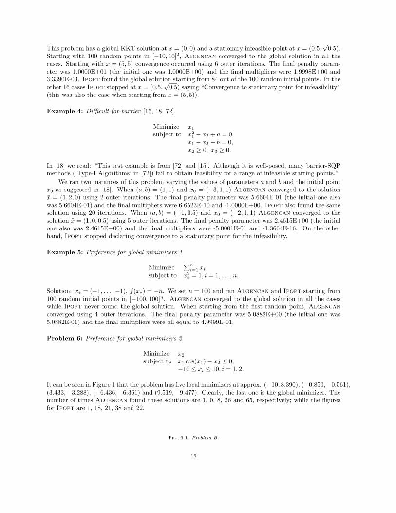
Problem 6: Preference for global minimizers 2

Minimize x2

subject to x1 cos(x1)− x2 ≤ 0,−10 ≤ xi ≤ 10, i = 1, 2.

It can be seen in Figure 1 that the problem has five local minimizers at approx. (−10, 8.390), (−0.850,−0.561),(3.433,−3.288), (−6.436,−6.361) and (9.519,−9.477). Clearly, the last one is the global minimizer. Thenumber of times Algencan found these solutions are 1, 0, 8, 26 and 65, respectively; while the figuresfor Ipopt are 1, 18, 21, 38 and 22.

Fig. 6.1. Problem B.

16

6.2. Problems with many inequality constraints. Consider the hard-spheres problem [50]:

Minimize zsubject to 〈vi, vj〉 ≤ z, i = 1, . . . , np, j = i + 1, . . . , np,

‖vi‖22 = 1, i = 1, . . . , np,

where vi ∈ IRnd for all i = 1, . . . , np. This problem has nd×np+1 variables, np equality constraints andnp× (np− 1)/2 inequality constraints.

For this particular problem, we ran Algencan with the Fortran formulation of the problem, Lancelot Bwith the SIF formulation and Ipopt with the AMPL formulation. In all cases we used analytic secondderivatives and the same random initial point, as we coded a Fortran 77 program that generates SIFand AMPL formulations that include the initial point. The motivation for this choice was that, althoughthe reasons are not clear for us, the combination of Algencan with the AMPL formulation was veryslow (this was not the case in the other problems) and the combination of Lancelot with AMPL gavethe error message “[...] failure: ran out of memory” for np ≥ 180. The combination of Ipopt withAMPL worked well and gave an average behavior almost identical to the combination of Ipopt with theFortran 77 formulation of the problem. We are aware that these different computer environments mayhave some influence in the interpretation of the results. However, we think that the numerical resultsindicate the essential correctness of the many-inequalities claim.

For Lancelot B (and Lancelot, which will appear in further experiments) we used all its defaultparameters and the same stopping criterion as Algencan, i.e., 10−4 for the feasibility and optimalitytolerances measured in the sup-norm. This may be considered as a rather large feasibility-optimalitytolerance. In fact, Augmented Lagrangian methods do not have fast local convergence. If we ask for morestrict tolerances, the performance of the Augmented Lagrangian methods deteriorate in comparison to theone of Ipopt.

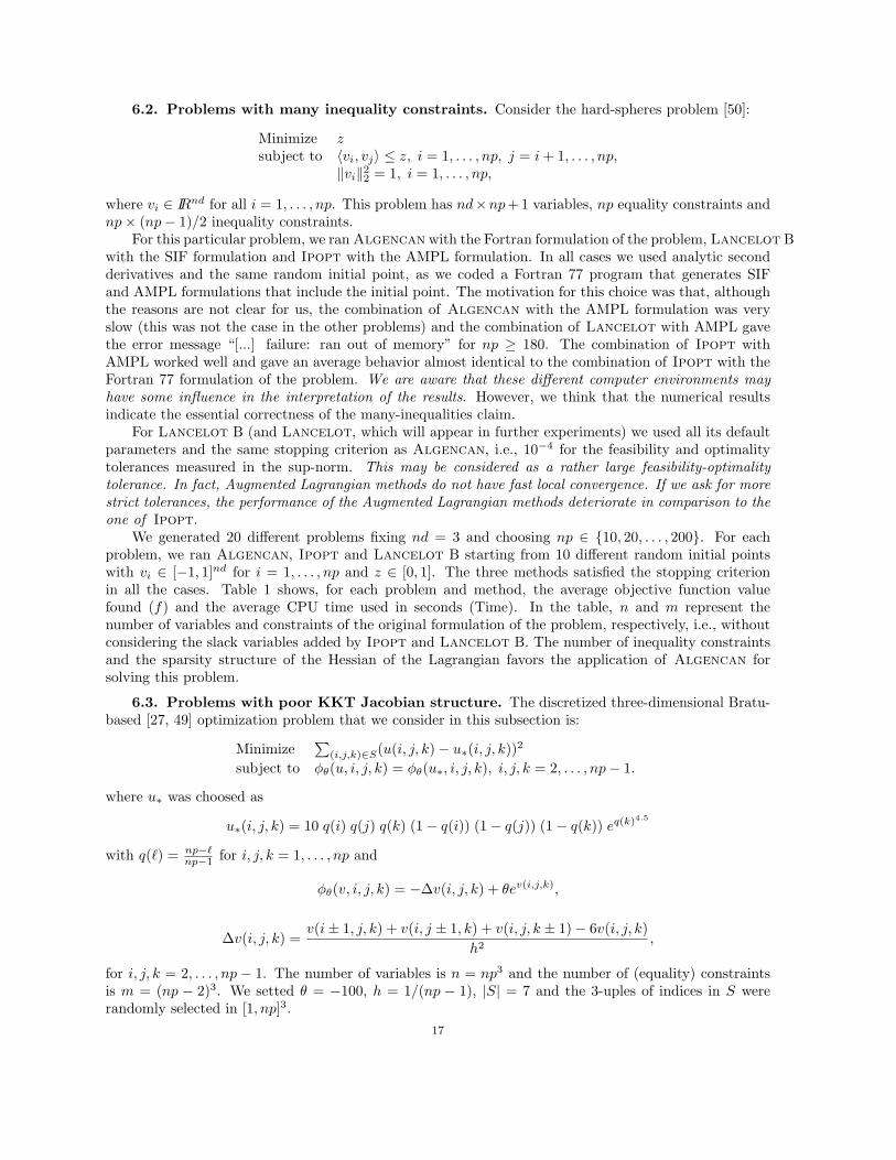
We generated 20 different problems fixing nd = 3 and choosing np ∈ 10, 20, . . . , 200. For eachproblem, we ran Algencan, Ipopt and Lancelot B starting from 10 different random initial pointswith vi ∈ [−1, 1]nd for i = 1, . . . , np and z ∈ [0, 1]. The three methods satisfied the stopping criterionin all the cases. Table 1 shows, for each problem and method, the average objective function valuefound (f) and the average CPU time used in seconds (Time). In the table, n and m represent thenumber of variables and constraints of the original formulation of the problem, respectively, i.e., withoutconsidering the slack variables added by Ipopt and Lancelot B. The number of inequality constraintsand the sparsity structure of the Hessian of the Lagrangian favors the application of Algencan forsolving this problem.

6.3. Problems with poor KKT Jacobian structure. The discretized three-dimensional Bratu-based [27, 49] optimization problem that we consider in this subsection is:

Minimize∑

(i,j,k)∈S(u(i, j, k)− u∗(i, j, k))2

subject to φθ(u, i, j, k) = φθ(u∗, i, j, k), i, j, k = 2, . . . , np− 1.

where u∗ was choosed as

u∗(i, j, k) = 10 q(i) q(j) q(k) (1− q(i)) (1− q(j)) (1− q(k)) eq(k)4.5

with q(`) = np−`np−1 for i, j, k = 1, . . . , np and

φθ(v, i, j, k) = −∆v(i, j, k) + θev(i,j,k),

∆v(i, j, k) =v(i± 1, j, k) + v(i, j ± 1, k) + v(i, j, k ± 1)− 6v(i, j, k)

h2,

for i, j, k = 2, . . . , np − 1. The number of variables is n = np3 and the number of (equality) constraintsis m = (np − 2)3. We setted θ = −100, h = 1/(np − 1), |S| = 7 and the 3-uples of indices in S wererandomly selected in [1, np]3.

17

Algencan Ipopt Lancelot Bn m Time f Time f Time f

31 55 0.01 0.404687 0.04 0.408676 0.04 0.40924461 210 0.03 0.676472 0.28 0.676851 0.42 0.67647791 465 0.17 0.781551 1.08 0.783792 1.97 0.782241

121 820 0.47 0.837600 3.12 0.838449 6.79 0.839005151 1275 0.97 0.868312 9.26 0.869486 14.63 0.870644181 1830 1.65 0.889745 13.96 0.891025 38.08 0.891436211 2485 3.12 0.905335 30.87 0.905975 64.36 0.906334241 3240 4.14 0.917323 33.91 0.918198 109.88 0.918182271 4095 5.66 0.926429 44.03 0.927062 158.12 0.926889301 5050 7.75 0.933671 61.47 0.933892 289.92 0.934201331 6105 11.29 0.939487 84.18 0.939791 287.40 0.940192361 7260 16.48 0.944514 115.73 0.944651 386.92 0.945134391 8515 20.18 0.953824 171.56 0.948912 486.04 0.949213421 9870 24.99 0.952265 254.16 0.952398 842.10 0.952667451 11325 31.00 0.955438 259.74 0.955609 811.37 0.955943481 12880 35.04 0.958227 289.55 0.958325 1381.74 0.958654511 14535 42.10 0.960621 457.32 0.960682 1407.71 0.961051541 16290 48.94 0.962813 476.82 0.962837 1565.95 0.963113571 18145 57.83 0.964722 773.90 0.964795 1559.51 0.965159601 20100 68.52 0.969767 1155.17 0.966444 2480.00 0.966822

Table 6.1Performance of Algencan, Ipopt and Lancelot B in the hard-spheres problem.

Sixteen problems were generated setting np = 5, 6, . . . , 20. They were solved using Algencan, Ipoptand Lancelot (this problem was formulated in AMPL and Lancelot B has no AMPL interface). Theinitial point was randomly generated in [0, 1]n. The three methods found solutions with null objectivefunction value. Table 2 shows some figures that reflect the computational effort of the methods. Inthe table, “Outit” means number of outer iterations of an augmented Lagrangian method, “It” meansnumber of iterations (or inner iterations), “Fcnt” means number of functional evaluations, “Gcnt” meansnumber of gradient evaluations and “Time” means CPU time in seconds. In the table, n and m representthe number of variables1 and (equality) constraints of the problem. The poor sparsity structure of theHessian of the Lagrangian favors the application of Algencan for solving this problem.

The warnings in italics made with respect to the Hard-Spheres problem are also pertinent for thisproblem. In particular, remember that we use a non-exigent convergence criterion.

6.4. Location problems. Here we will consider a variant of the family of location problems intro-duced in [11]. In the original problem, given a set of np disjoint polygons P1, P2, . . . , Pnp in IR2 one wishesto find the point z1 ∈ P1 that minimizes the sum of the distances to the other polygons. Therefore, theoriginal problem formulation is:

minzi, i=1,...,np

1np− 1

np∑i=2

‖zi − z1‖2

subject to zi ∈ Pi, i = 1, . . . , np.

In the variant considered in the present work, we have, in addition to the np polygons, nc circles.Moreover, there is an ellipse which has a non empty intersection with P1 and such that z1 must be insidethe ellipse and zi, i = 2, . . . , np + nc must be outside. Therefore, the problem considered in this work is

minzi, i=1,...,np+nc

1nc + np− 1

[np∑i=2

‖zi − z1‖2 +nc∑i=1

‖znp+i − z1‖2

]1The AMPL presolver procedure eliminates some problem variables.

18

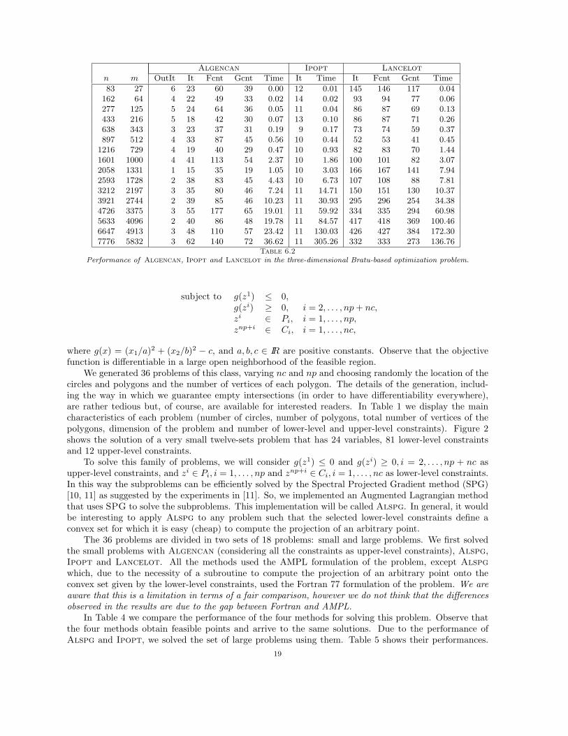
Algencan Ipopt Lancelotn m OutIt It Fcnt Gcnt Time It Time It Fcnt Gcnt Time

83 27 6 23 60 39 0.00 12 0.01 145 146 117 0.04162 64 4 22 49 33 0.02 14 0.02 93 94 77 0.06277 125 5 24 64 36 0.05 11 0.04 86 87 69 0.13433 216 5 18 42 30 0.07 13 0.10 86 87 71 0.26638 343 3 23 37 31 0.19 9 0.17 73 74 59 0.37897 512 4 33 87 45 0.56 10 0.44 52 53 41 0.45

1216 729 4 19 40 29 0.47 10 0.93 82 83 70 1.441601 1000 4 41 113 54 2.37 10 1.86 100 101 82 3.072058 1331 1 15 35 19 1.05 10 3.03 166 167 141 7.942593 1728 2 38 83 45 4.43 10 6.73 107 108 88 7.813212 2197 3 35 80 46 7.24 11 14.71 150 151 130 10.373921 2744 2 39 85 46 10.23 11 30.93 295 296 254 34.384726 3375 3 55 177 65 19.01 11 59.92 334 335 294 60.985633 4096 2 40 86 48 19.78 11 84.57 417 418 369 100.466647 4913 3 48 110 57 23.42 11 130.03 426 427 384 172.307776 5832 3 62 140 72 36.62 11 305.26 332 333 273 136.76

Table 6.2Performance of Algencan, Ipopt and Lancelot in the three-dimensional Bratu-based optimization problem.

subject to g(z1) ≤ 0,g(zi) ≥ 0, i = 2, . . . , np + nc,zi ∈ Pi, i = 1, . . . , np,znp+i ∈ Ci, i = 1, . . . , nc,

where g(x) = (x1/a)2 + (x2/b)2 − c, and a, b, c ∈ IR are positive constants. Observe that the objectivefunction is differentiable in a large open neighborhood of the feasible region.

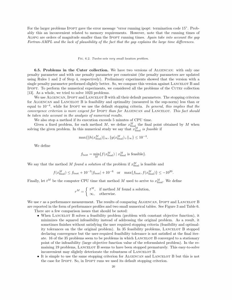
We generated 36 problems of this class, varying nc and np and choosing randomly the location of thecircles and polygons and the number of vertices of each polygon. The details of the generation, includ-ing the way in which we guarantee empty intersections (in order to have differentiability everywhere),are rather tedious but, of course, are available for interested readers. In Table 1 we display the maincharacteristics of each problem (number of circles, number of polygons, total number of vertices of thepolygons, dimension of the problem and number of lower-level and upper-level constraints). Figure 2shows the solution of a very small twelve-sets problem that has 24 variables, 81 lower-level constraintsand 12 upper-level constraints.

To solve this family of problems, we will consider g(z1) ≤ 0 and g(zi) ≥ 0, i = 2, . . . , np + nc asupper-level constraints, and zi ∈ Pi, i = 1, . . . , np and znp+i ∈ Ci, i = 1, . . . , nc as lower-level constraints.In this way the subproblems can be efficiently solved by the Spectral Projected Gradient method (SPG)[10, 11] as suggested by the experiments in [11]. So, we implemented an Augmented Lagrangian methodthat uses SPG to solve the subproblems. This implementation will be called Alspg. In general, it wouldbe interesting to apply Alspg to any problem such that the selected lower-level constraints define aconvex set for which it is easy (cheap) to compute the projection of an arbitrary point.

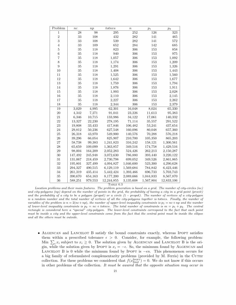
The 36 problems are divided in two sets of 18 problems: small and large problems. We first solvedthe small problems with Algencan (considering all the constraints as upper-level constraints), Alspg,Ipopt and Lancelot. All the methods used the AMPL formulation of the problem, except Alspgwhich, due to the necessity of a subroutine to compute the projection of an arbitrary point onto theconvex set given by the lower-level constraints, used the Fortran 77 formulation of the problem. We areaware that this is a limitation in terms of a fair comparison, however we do not think that the differencesobserved in the results are due to the gap between Fortran and AMPL.

In Table 4 we compare the performance of the four methods for solving this problem. Observe thatthe four methods obtain feasible points and arrive to the same solutions. Due to the performance ofAlspg and Ipopt, we solved the set of large problems using them. Table 5 shows their performances.

19

For the larger problems Ipopt gave the error message “error running ipopt: termination code 15”. Prob-ably this an inconvenient related to memory requirements. However, note that the running times ofAlspg are orders of magnitude smaller than the Ipopt running times. Again take into account the gapFortran-AMPL and the lack of plausibility of the fact that the gap explains the large time differences.

Fig. 6.2. Twelve-sets very small location problem.

6.5. Problems in the Cuter collection. We have two versions of Algencan: with only onepenalty parameter and with one penalty parameter per constraint (the penalty parameters are updatedusing Rules 1 and 2 of Step 4, respectively). Preliminary experiments showed that the version with asingle penalty parameter performed slightly better. So, we compare this version against Lancelot B andIpopt. To perform the numerical experiments, we considered all the problems of the Cuter collection[13]. As a whole, we tried to solve 1023 problems.

We use Algencan, Ipopt and Lancelot B with all their default parameters. The stopping criterionfor Algencan and Lancelot B is feasibility and optimality (measured in the sup-norm) less than orequal to 10−4, while for Ipopt we use the default stopping criteria. In general, this implies that theconvergence criterion is more exigent for Ipopt than for Algencan and Lancelot. This fact shouldbe taken into account in the analysis of numerical results.

We also stop a method if its execution exceeds 5 minutes of CPU time.Given a fixed problem, for each method M , we define xM

final the final point obtained by M whensolving the given problem. In this numerical study we say that xM

final is feasible if

max‖h(xMfinal)‖∞, ‖g(xM

final)+‖∞ ≤ 10−4.

We define

fbest = minMf(xM

final) | xMfinal is feasible.

We say that the method M found a solution of the problem if xMfinal is feasible and

f(xMfinal) ≤ fbest + 10−3|fbest|+ 10−6 or maxfbest, f(xM

final) ≤ −1020.

Finally, let tM be the computer CPU time that method M used to arrive to xMfinal. We define

rM =

tM , if method M found a solution,∞, otherwise.

We use r as a performance measurement. The results of comparing Algencan, Ipopt and Lancelot Bare reported in the form of performance profiles and two small numerical tables. See Figure 3 and Table 6.

There are a few comparison issues that should be noted:• When Lancelot B solves a feasibility problem (problem with constant objective function), it

minimizes the squared infeasibility instead of addressing the original problem. As a result, itsometimes finishes without satisfying the user required stopping criteria (feasibility and optimal-ity tolerances on the the original problem). In 35 feasibility problems, Lancelot B stoppeddeclaring convergence but the user-required feasibility tolerance is not satisfied at the final iter-ate. 16 of the 35 problems seem to be problems in which Lancelot B converged to a stationarypoint of the infeasibility (large objective function value of the reformulated problem). In the re-maining 19 problems, Lancelot B seems to have been stopped prematurely. This easy-to-solveinconvenient may slightly deteriorate the robustness of Lancelot B.• It is simple to use the same stopping criterion for Algencan and Lancelot B but this is not

the case for Ipopt. So, in Ipopt runs we used its default stopping criterion.20

Problem nc np totnvs n p1 p2

1 28 98 295 252 126 3232 33 108 432 282 141 4653 33 108 539 282 141 5724 33 109 652 284 142 6855 35 118 823 306 153 8586 35 118 940 306 153 9757 35 118 1,057 306 153 1,0928 35 118 1,174 306 153 1,2099 35 118 1,291 306 153 1,32610 35 118 1,408 306 153 1,44311 35 118 1,525 306 153 1,56012 35 118 1,642 306 153 1,67713 35 118 1,759 306 153 1,79414 35 118 1,876 306 153 1,91115 35 118 1,993 306 153 2,02816 35 118 2,110 306 153 2,14517 35 118 2,227 306 153 2,26218 35 118 2,344 306 153 2,379

19 3,029 4,995 62,301 16,048 8,024 65,33020 4,342 7,271 91,041 23,226 11,613 95,38321 6,346 10,715 133,986 34,122 17,061 140,33222 13,327 22,230 278,195 71,114 35,557 291,52223 19,808 33,433 417,846 106,482 53,241 437,65424 29,812 50,236 627,548 160,096 80,048 657,36025 26,318 43,970 549,900 140,576 70,288 576,21826 39,296 66,054 825,907 210,700 105,350 865,20327 58,738 99,383 1,241,823 316,242 158,121 1,300,56128 65,659 109,099 1,363,857 349,516 174,758 1,429,51629 98,004 164,209 2,052,283 524,426 262,213 2,150,28730 147,492 245,948 3,072,630 786,880 393,440 3,220,12231 131,067 218,459 2,730,798 699,052 349,526 2,861,86532 195,801 327,499 4,094,827 1,046,600 523,300 4,290,62833 294,327 490,515 6,129,119 1,569,684 784,842 6,423,44634 261,319 435,414 5,442,424 1,393,466 696,733 5,703,74335 390,670 654,163 8,177,200 2,089,666 1,044,833 8,567,87036 588,251 979,553 12,244,855 3,135,608 1,567,804 12,833,106

Table 6.3Location problems and their main features. The problem generation is based on a grid. The number of city-circles (nc)

and city-polygons (np) depend on the number of points in the grid, the probability of having a city in a grid point (procit)and the probability of a city to be a polygon (propol) or a circle (1 − propol). The number of vertices of a city-polygonis a random number and the total number of vertices of all the city-polygons together is totnvs. Finally, the number ofvariables of the problem is n = 2(nc+np), the number of upper-level inequality constraints is p1 = nc+np and the numberof lower-level inequality constraints is p2 = nc + totnvs. The total number of constraints is m = p1 + p2. The centralrectangle is considered here a “special” city-polygon. The lower-level constraints correspond to the fact that each pointmust be inside a city and the upper-level constraints come from the fact that the central point must be inside the ellipseand all the others must be outside.

• Algencan and Lancelot B satisfy the bound constraints exactly, whereas Ipopt satisfiesthem within a prescribed tolerance ε > 0. Consider, for example, the following problem:Min

∑i xi subject to xi ≥ 0. The solution given by Algencan and Lancelot B is the ori-

gin, while the solution given by Ipopt is xi = −ε. So, the minimum found by Algencan andLancelot B is 0 while the minimum found by Ipopt is −εn. This phenomenon occurs fora big family of reformulated complementarity problems (provided by M. Ferris) in the Cutercollection. For these problems we considered that f(xIpopt

final ) = 0. We do not know if this occursin other problems of the collection. It must be awared that the opposite situation may occur in

21

Problem CPU Time (secs.) fAlgencan Alspg Ipopt Lancelot

1 1.53 0.06 0.11 854.82 1.7564E+012 2.17 0.11 0.13 319.24 1.7488E+013 2.25 0.14 0.14 401.08 1.7466E+014 1.71 0.12 0.17 139.60 1.7451E+015 1.75 0.11 0.19 129.79 1.7984E+016 1.83 0.09 0.21 90.37 1.7979E+017 2.18 0.08 0.23 72.14 1.7975E+018 1.88 0.08 0.28 92.74 1.7971E+019 1.84 0.18 0.29 111.13 1.7972E+0110 2.06 0.14 0.37 100.23 1.7969E+0111 2.18 0.13 0.49 86.54 1.7969E+0112 2.55 0.16 0.50 134.23 1.7968E+0113 2.39 0.18 0.37 110.28 1.7968E+0114 2.52 0.20 0.42 223.05 1.7965E+0115 2.63 0.17 0.61 657.99 1.7965E+0116 3.36 0.18 0.44 672.01 1.7965E+0117 2.99 0.17 0.46 505.00 1.7963E+0118 3.43 0.23 0.48 422.93 1.7963E+01

Table 6.4Performance of Algencan, Alspg, Ipopt and Lancelot in the set of small location problems.

other problems of the collection. Namely, since we use a weak stopping feasibility criterion for theAugmented Lagrangian methods, it is possible that the objective function value of an AugmentedLagrangian method is artificially smaller than the objective function value obtained by Ipoptinsome (perhaps many) problems. The numerical results presented here should be analyzed withthis objection in mind.• We have good reasons for defining the initial penalty parameter ρ1 as stated at the beginning of

this section. However, in many problems of the Cuter collection, ρ1 = 10 behaves better. Forthis reason we include the statistics also for the non-default choice ρ1 = 10.

We detected 73 problems in which both Algencan and Ipopt finished declaring that the optimalsolution was found but found different functional values. In 58 of these problems the functional valueobtained by Algencan was smaller than the one found by Ipopt. This may confirm the conjecture thatthe Augmented Lagrangian method has a stronger tendency towards global optimality than interior-SQPmethods but it must also be taken into account the possibility of an unfair functional value comparisondue to the different tolerances used.

Fig. 6.3. Performance profiles of Algencan, Lancelot B and Ipopt in the problems of the Cuter collection. Notethat there is a CPU time limit of 5 minutes for each pair method/problem. The second graphic is a zoom of the left-handside of the first one. Although in the Cuter test set of problems Algencan with ρ1 = 10 performs better (see Table 6)than using the choice of ρ1 stated at the begining of this section, we used the last option (which is the Algencan defaultoption) to build the performance profiles curves in this graphics.

6.6. Additional detailed tests with Algencan. In this section we report in detail some specifictests, where we compare Algencan against Ipopt. In these tests we always use the default parameteresfor both methods. As stopping convergence tolerance we use 10−8 in both methods. In particular,εfeas = εopt = 10−8 in Algencan.

22

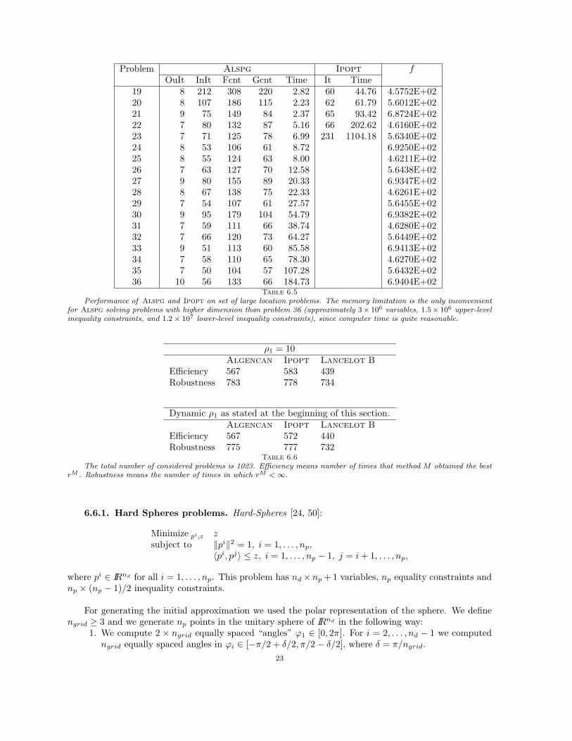
Problem Alspg Ipopt fOuIt InIt Fcnt Gcnt Time It Time

19 8 212 308 220 2.82 60 44.76 4.5752E+0220 8 107 186 115 2.23 62 61.79 5.6012E+0221 9 75 149 84 2.37 65 93.42 6.8724E+0222 7 80 132 87 5.16 66 202.62 4.6160E+0223 7 71 125 78 6.99 231 1104.18 5.6340E+0224 8 53 106 61 8.72 6.9250E+0225 8 55 124 63 8.00 4.6211E+0226 7 63 127 70 12.58 5.6438E+0227 9 80 155 89 20.33 6.9347E+0228 8 67 138 75 22.33 4.6261E+0229 7 54 107 61 27.57 5.6455E+0230 9 95 179 104 54.79 6.9382E+0231 7 59 111 66 38.74 4.6280E+0232 7 66 120 73 64.27 5.6449E+0233 9 51 113 60 85.58 6.9413E+0234 7 58 110 65 78.30 4.6270E+0235 7 50 104 57 107.28 5.6432E+0236 10 56 133 66 184.73 6.9404E+02

Table 6.5Performance of Alspg and Ipopt on set of large location problems. The memory limitation is the only inconvenient

for Alspg solving problems with higher dimension than problem 36 (approximately 3× 106 variables, 1.5× 106 upper-levelinequality constraints, and 1.2× 107 lower-level inequality constraints), since computer time is quite reasonable.

ρ1 = 10Algencan Ipopt Lancelot B

Efficiency 567 583 439Robustness 783 778 734

Dynamic ρ1 as stated at the beginning of this section.Algencan Ipopt Lancelot B

Efficiency 567 572 440Robustness 775 777 732

Table 6.6The total number of considered problems is 1023. Efficiency means number of times that method M obtained the best

rM . Robustness means the number of times in which rM <∞.

6.6.1. Hard Spheres problems. Hard-Spheres [24, 50]:

Minimize pi,z zsubject to ‖pi‖2 = 1, i = 1, . . . , np,

〈pi, pj〉 ≤ z, i = 1, . . . , np − 1, j = i + 1, . . . , np,

where pi ∈ IRnd for all i = 1, . . . , np. This problem has nd×np + 1 variables, np equality constraints andnp × (np − 1)/2 inequality constraints.

For generating the initial approximation we used the polar representation of the sphere. We definengrid ≥ 3 and we generate np points in the unitary sphere of IRnd in the following way:

1. We compute 2 × ngrid equally spaced “angles” ϕ1 ∈ [0, 2π]. For i = 2, . . . , nd − 1 we computedngrid equally spaced angles in ϕi ∈ [−π/2 + δ/2, π/2− δ/2], where δ = π/ngrid.

23

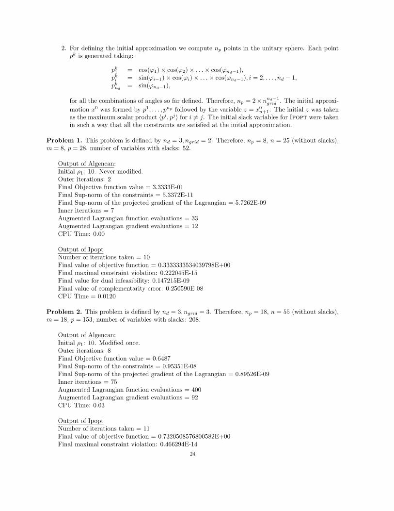
2. For defining the initial approximation we compute np points in the unitary sphere. Each pointpk is generated taking:

pk1 = cos(ϕ1)× cos(ϕ2)× . . .× cos(ϕnd−1),

pki = sin(ϕi−1)× cos(ϕi)× . . .× cos(ϕnd−1), i = 2, . . . , nd − 1,

pknd

= sin(ϕnd−1),

for all the combinations of angles so far defined. Therefore, np = 2×nnd−1grid . The initial approxi-

mation x0 was formed by p1, . . . , pnp followed by the variable z = x0n+1. The initial z was taken

as the maximum scalar product 〈pi, pj〉 for i 6= j. The initial slack variables for Ipopt were takenin such a way that all the constraints are satisfied at the initial approximation.

Problem 1. This problem is defined by nd = 3, ngrid = 2. Therefore, np = 8, n = 25 (without slacks),m = 8, p = 28, number of variables with slacks: 52.

Output of Algencan:Initial ρ1: 10. Never modified.Outer iterations: 2Final Objective function value = 3.3333E-01Final Sup-norm of the constraints = 5.3372E-11Final Sup-norm of the projected gradient of the Lagrangian = 5.7262E-09Inner iterations = 7Augmented Lagrangian function evaluations = 33Augmented Lagrangian gradient evaluations = 12CPU Time: 0.00

Output of IpoptNumber of iterations taken = 10Final value of objective function = 0.3333333534039798E+00Final maximal constraint violation: 0.222045E-15Final value for dual infeasibility: 0.147215E-09Final value of complementarity error: 0.250590E-08CPU Time = 0.0120


Output of Algencan:Initial ρ1: 10. Modified once.Outer iterations: 8Final Objective function value = 0.6487Final Sup-norm of the constraints = 0.95351E-08Final Sup-norm of the projected gradient of the Lagrangian = 0.89526E-09Inner iterations = 75Augmented Lagrangian function evaluations = 400Augmented Lagrangian gradient evaluations = 92CPU Time: 0.03

Output of IpoptNumber of iterations taken = 11Final value of objective function = 0.7320508576800582E+00Final maximal constraint violation: 0.466294E-14

24

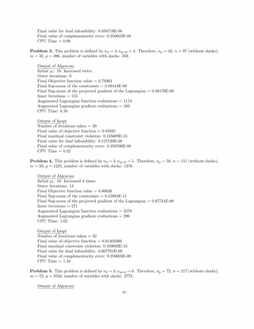
Final value for dual infeasibility: 0.456718E-08Final value of complementarity error: 0.250602E-08CPU Time = 0.06


Output of Algencan:Initial ρ1: 10. Increased twice.Outer iterations: 6Final Objective function value = 0.79362Final Sup-norm of the constraints = 0.89444E-09Final Sup-norm of the projected gradient of the Lagrangian = 0.38170E-08Inner iterations = 155Augmented Lagrangian function evaluations = 1174Augmented Lagrangian gradient evaluations = 169CPU Time: 0.16

Output of IpoptNumber of iterations taken = 20Final value of objective function = 0.85935Final maximal constraint violation: 0.135689E-13Final value for dual infeasibility: 0.155720E-08Final value of complementarity error: 0.250590E-08CPU Time = 0.32


Output of Algencan:Initial ρ1: 10. Increased 4 times.Outer iterations: 12Final Objective function value = 0.86826Final Sup-norm of the constraints = 0.15984E-11Final Sup-norm of the projected gradient of the Lagrangian = 0.87741E-08Inner iterations = 271Augmented Lagrangian function evaluations = 2478Augmented Lagrangian gradient evaluations = 296CPU Time: 1.02



Output of Algencan:25

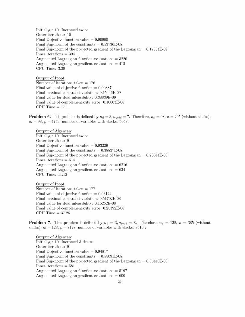
Initial ρ1: 10. Increased twice.Outer iterations: 10Final Objective function value = 0.90900Final Sup-norm of the constraints = 0.53736E-08Final Sup-norm of the projected gradient of the Lagrangian = 0.17834E-09Inner iterations = 394Augmented Lagrangian function evaluations = 3220Augmented Lagrangian gradient evaluations = 415CPU Time: 3.29



Output of Algencan:Initial ρ1: 10. Increased twice.Outer iterations: 9Final Objective function value = 0.93229Final Sup-norm of the constraints = 0.38827E-08Final Sup-norm of the projected gradient of the Lagrangian = 0.23044E-08Inner iterations = 614Augmented Lagrangian function evaluations = 6216Augmented Lagrangian gradient evaluations = 634CPU Time: 11.12


Problem 7. This problem is defined by nd = 3, ngrid = 8. Therefore, np = 128, n = 385 (withoutslacks), m = 128, p = 8128, number of variables with slacks: 8513 .

Output of Algencan:Initial ρ1: 10. Increased 3 times.Outer iterations: 9Final Objective function value = 0.94817Final Sup-norm of the constraints = 0.55091E-08Final Sup-norm of the projected gradient of the Lagrangian = 0.35440E-08Inner iterations = 581Augmented Lagrangian function evaluations = 5197Augmented Lagrangian gradient evaluations = 600

26

CPU Time: 23.55


Problem 8. This problem is defined by nd = 3, ngrid = 9. Therefore, np = 162, n = 487 (withoutslacks), m = 162, p = 13041, number of variables with slacks: 13528.

Output of Algencan:Initial ρ1: 10. Increased 3 times.Outer iterations: 9Final Objective function value = 0.95895Final Sup-norm of the constraints = 0.39203E-08Final Sup-norm of the projected gradient of the Lagrangian = 0.33077E-08Inner iterations = 857Augmented Lagrangian function evaluations = 9119Augmented Lagrangian gradient evaluations = 876CPU Time: 56.96



Output of Algencan:Initial ρ1: 10. Increased 3 times.Outer iterations: 10Final Objective function value = 0.96645E-01Final Sup-norm of the constraints = 0.24079E-09Final Sup-norm of the projected gradient of the Lagrangian = 0.42462E-08Inner iterations = 865Augmented Lagrangian function evaluations = 8699Augmented Lagrangian gradient evaluations = 886CPU Time: 91.69

Output of IpoptNumber of iterations taken = 735Final value of objective function = 0.96643Final maximal constraint violation: 0.12885E-08Final value for dual infeasibility: 0.45514E-10Final value of complementarity error: 0.10018E-08

27

CPU Time = 2467.39


Output of Algencan:Initial ρ1: 10. Never modified.Outer iterations: 2Final Objective function value = 5.0000E-01Final Sup-norm of the constraints = 7.1044E-11Final Sup-norm of the projected gradient of the Lagrangian = 2.0461E-10Inner iterations = 11Augmented Lagrangian function evaluations = 45Augmented Lagrangian gradient evaluations = 16CPU Time: 0.00



Output of Algencan:Initial ρ1: 10. Incremented 3 times.Outer iterations: 10Final Objective function value = 7.1601E-01Final Sup-norm of the constraints = 3.0697E-12Final Sup-norm of the projected gradient of the Lagrangian = 2.3415E-09Inner iterations = 686Augmented Lagrangian function evaluations = 6878Augmented Lagrangian gradient evaluations = 707CPU Time: 3.41



Output of Algencan:Initial ρ1: 10. Incremented 5 times.Outer iterations: 14

28

Final Objective function value = 8.3620E-01Final Sup-norm of the constraints = 1.4941E-12Final Sup-norm of the projected gradient of the Lagrangian = 2.7177E-09Inner iterations = 1786Augmented Lagrangian function evaluations = 17363Augmented Lagrangian gradient evaluations = 1816CPU Time: 57.26







29


6.6.2. Enclosing-Ellipsoid problems [69].

Minimize lij−

∑nd

i=1 log(lii)subject to (pi)T LLT pi ≤ 1, i = 1, ..., np,

lii ≥ 10−16, i = 1, ..., nd,

where L ∈ IRnd×nd is a lower-triangular matrix. The number of variables is nd × (nd + 1)/2 and thenumber of inequality constraints is np (plus the bound constraints).

In this version of the problem, instead of randomly generated the np points pi ∈ IRnd using the Cauchydistribution as suggested in [69], we consider the 4278 atoms of a 3D protein of the Isoform alpha of theThyroid Hormone Receptor. (Their exact location can be found in nonlinear programming problems col-lection “La Cumparsita” accessible through the TANGO Project web page http://www.ime.usp.br/∼egbirgin/tango/.)

This problem has n = 6 (without slacks), m = 0, p = 4278, number of variables with slacks: 4284.

Output of Algencan:Initial ρ1: 10. Incremented once.Outer iterations: 22Final Objective function value = 1.0220E+01Final Sup-norm of the constraints = 1.6405E-09Final Sup-norm of the projected gradient of the Lagrangian = 1.0988E-12Inner iterations = 89Augmented Lagrangian function evaluations = 145Augmented Lagrangian gradient evaluations = 134CPU Time: 0.34


6.6.3. Full Discretized three-dimensional Bratu-based problem. [27, 49]:

Minimize u(i,j,k)

∑i,j,k u(i, j, k)2

subject to φθ(u, i, j, k) = φθ(u∗, i, j, k), i, j, k = 2, . . . , np − 1.

where u∗ is defined by

u∗(i, j, k) = 10 q(i) q(j) q(k) (1− q(i)) (1− q(j)) (1− q(k)) eq(k)4.5,

for i, j, k = 1, 2, . . . , np, with q(`) = (np − `)/(np − 1) for all ` = 1, 2, . . . , np,

φθ(v, i, j, k) = −∆v(i, j, k) + θev(i,j,k),

30

and

∆v(i, j, k) =v(i± 1, j, k) + v(i, j ± 1, k) + v(i, j, k ± 1)− 6v(i, j, k)

h2,

for i, j, k = 2, . . . , np−1. The number of variables is n3p and the number of equality constraints is (np−2)3.

We set θ = −100, h = 1/(np− 1). This problem has no inequality constraints. The initial approximationis u ≡ 0.

Problem BF1. This problem is defined by np = 10. Therefore, n = 1000, m = 512.

Output of Algencan:Initial ρ1: 1.0186E-03. Incremented once.Outer iterations: 14Final Objective function value = 3.2054E+00Final Sup-norm of the constraints = 5.3281E-09Final Sup-norm of the projected gradient of the Lagrangian = 8.1686E-09Inner iterations = 58Augmented Lagrangian function evaluations = 527Augmented Lagrangian gradient evaluations = 87CPU Time: 0.60

Output of IpoptNumber of iterations taken = 4Final value of objective function = 0.3205420550537569E+01Final maximal constraint violation: 0.354476E-08Final value for dual infeasibility: 0.207779E-09CPU Time = 0.12


Output of Algencan:Initial ρ1: 2.1702E-04. Incremented 5 times.Outer iterations: 21Final Objective function value = 1.5075E+01Final Sup-norm of the constraints = 1.1149E-09Final Sup-norm of the projected gradient of the Lagrangian = 9.2846E-09Inner iterations = 83Augmented Lagrangian function evaluations = 866Augmented Lagrangian gradient evaluations = 126CPU Time: 7.66



Output of Algencan:Initial ρ1: 1.0583E-04. Incremented twice.

31

Outer iterations: 23Final Objective function value = 3.0716E+01Final Sup-norm of the constraints = 8.3196E-09Final Sup-norm of the projected gradient of the Lagrangian = 1.0207E-09Inner iterations = 98Augmented Lagrangian function evaluations = 913Augmented Lagrangian gradient evaluations = 145CPU Time: 27.72


In the following problems we replaced the objective function of the previous problem by zero. So,the following problems are, in fact, feasibility problems.

Problem BZ1. This problem is defined by np = 10. Therefore, n = 1000, m = 512.

Output of Algencan:Initial ρ1: 1.0186E-03. Never incremented.Outer iterations: 1Final Objective function value = 0.0000E+00Final Sup-norm of the constraints = 8.6310E-09Final Sup-norm of the projected gradient of the Lagrangian = 1.2367E-09Inner iterations = 5Augmented Lagrangian function evaluations = 9Augmented Lagrangian gradient evaluations = 8CPU Time: 0.04



Output of Algencan:Initial ρ1: 2.1702E-04. Never incremented.Outer iterations: 1Final Objective function value = 0.0000E+00Final Sup-norm of the constraints = 6.6840E-09Final Sup-norm of the projected gradient of the Lagrangian = 6.9867E-10Inner iterations = 6Augmented Lagrangian function evaluations = 17Augmented Lagrangian gradient evaluations = 9CPU Time: 0.48

32



Output of Algencan:Initial ρ1: 2.1702E-04. Incremented twice.Outer iterations: 4Final Objective function value = 0.0000E+00Final Sup-norm of the constraints = 2.1731E-09Final Sup-norm of the projected gradient of the Lagrangian = 5.1446E-09Inner iterations = 7Augmented Lagrangian function evaluations = 25Augmented Lagrangian gradient evaluations = 16CPU Time: 1.85


Problem BZ4. This problem is defined by np = 30. Therefore, n = 27, 000, m = 21, 952.



Finally, we run a few more BZ problems with algencan:


Output of Algencan:33

Initial ρ1: 1.1923E-05. Incremented twice.Outer iterations: 4Final Objective function value = 0.0000E+00Final Sup-norm of the constraints = 2.5156E-09Final Sup-norm of the projected gradient of the Lagrangian = 1.9272E-09Inner iterations = 6Augmented Lagrangian function evaluations = 19Augmented Lagrangian gradient evaluations = 15CPU Time: 69.17




Output of Algencan:Initial ρ1: 3.4055E-06. Incremented once.Outer iterations: 3Final Objective function value = 0.0000E+00Final Sup-norm of the constraints = 5.7185E-09Final Sup-norm of the projected gradient of the Lagrangian = 1.3931E-10Inner iterations = 6Augmented Lagrangian function evaluations = 13Augmented Lagrangian gradient evaluations = 13CPU Time: 614.63



34

7. Final Remarks. In the last few years many sophisticated algorithms for nonlinear programminghave been published. They usually involve combinations of interior-point techniques, sequential quadraticprogramming, trust regions [23], restoration, nonmonotone strategies and advanced sparse linear algebraprocedures. See, for example [17, 39, 41, 42, 43, 53] and the extensive reference lists of these papers.Moreover, methods for solving efficiently specific problems or for dealing with special constraints areoften introduced. Many times, a particular algorithm is extremely efficient for dealing with problemsof a given type, but fails (or cannot be applied) when constraints of a different class are incorporated.Unfortunately, this situation is quite common in engineering applications. In the Augmented Lagrangianframework additional constraints are naturally incorporated to the objective function of the subproblems,which therefore preserve their constraint structure. For this reason, we conjecture that the AugmentedLagrangian approach (with general lower-level constraints) will continue to be used for many years.

This fact motivated us to improve and analyze Augmented Lagrangian methods with arbitrary lower-level constraints. From the theoretical point of view our goal was to eliminate, as much as possible,restrictive constraint qualifications. With this in mind we used, both in the feasibility proof and in theoptimality proof, the Constant Positive Linear Dependence (CPLD) condition. This condition [60] hasbeen proved to be a constraint qualification in [3] where its relations with other constraint qualificationshave been given.

We provided a family of examples (Location Problems) where the potentiality of the arbitrary lower-level approach is clearly evidenced. This example represents a typical situation in applications. A specificalgorithm (SPG) is known to be very efficient for a class of problems but turns out to be impossible toapply when additional constraints are incorporated. Fortunately, the Augmented Lagrangian approachis able to deal with the additional constraints taking advantage of the efficiency of SPG for solvingthe subproblems. In this way, we were able to solve nonlinear programming problems with more than3,000,000 variables and 14,000,000 constraints in less than five minutes of CPU time.

Many interesting open problems remain:1. The constraint qualification used for obtaining boundedness of the penalty parameter (regularity

at the limit point) is still too strong. We conjecture that it is possible to obtain the same resultusing the Mangasarian-Fromovitz constraint qualification.

2. The inexact-Newton approach employed by Gencan for solving box-constrained subproblemsdoes not seem to be affected by the nonexistence of second derivatives of the Augmented La-grangian for inequality constrained problems. There are good reasons to conjecture that thisis not the case when the box-constrained subproblem is solved using a quasi-Newton approach.This fact stimulates the development of efficient methods for minimizing functions with first (butnot second) derivatives.

3. The implementation of Augmented Lagrangian methods (as well as other nonlinear programmingalgorithms) is subject to many decisions on the parameters to be employed. Some of thesedecisions are not easy to take and one is compelled to use parameters largely based on experience.Theoretical criteria for deciding the best values of many parameters need to be developed.

4. In [2] an Augmented Lagrangian algorithm with many penalty parameters for single (box) lower-level constraints was analyzed and boundedness of the penalty parameters was proved withoutstrict complementarity assumptions. The generalization of that proof to the general lower-levelconstraints case considered here is not obvious and the existence of such generalization remainsan open problem.

5. Acceleration and warm-start procedures must be developed in order to speed the ultimate rateof convergence and to take advantage of the solution obtained for slightly different optimizationproblems.

AcknowledgementWe are indebted to Prof. A. R. Conn, whose comments on a first version of this paper guided a deep

revision.

REFERENCES

35

[1] M. Argaez and R. A. Tapia, On the global convergence of a modified augmented Lagrangian linesearch interior-pointmethod for Nonlinear Programming, Journal of Optimization Theory and Applications 114 (2002), pp. 1-25.

[2] R. Andreani, E. G. Birgin, J. M. Martınez and M. L. Schuverdt, Augmented Lagrangian Methods underthe Constant Positive Linear Dependence Constraint Qualification, Technical Report MCDO-040806 (seewww.ime.usp.br/∼egbirgin), Department of Applied Mathematics, UNICAMP, Brazil, 2004. To appear in Math-ematical Programming.

[3] R. Andreani, J. M. Martınez and M. L. Schuverdt, On the relation between the Constant Positive Linear Dependencecondition and quasinormality constraint qualification, Journal of Optimization Theory and Applications 125(2005), pp. 473-485. .

[4] S. Bakhtiari and A. L. Tits, A simple primal-dual feasible interior-point method for nonlinear programming withmonotone descent, Computational Optimization and Applications 25 (2003), pp. 17-38.

[5] D. P. Bertsekas, Constrained Optimization and Lagrange Multiplier Methods, Academic Press, 1982; republished byAthena Scientific, Belmont, Massachusetts, 1996.

[6] D. P. Bertsekas, Nonlinear Programming, 2nd edition, Athena Scientific, Belmont, Massachusetts, 1999.[7] E. G. Birgin, R. Castillo and J. M. Martınez, Numerical comparison of Augmented Lagrangian algorithms for non-

convex problems, Computational Optimization and Applications 31 (2005), pp. 31-56.[8] E. G. Birgin and J. M. Martınez, Structured minimal-memory inexact quasi-Newton method and secant preconditioners

for Augmented Lagrangian Optimization, submitted (2005).[9] E. G. Birgin and J. M. Martınez, Large-scale active-set box-constrained optimization method with spectral projected

gradients, Computational Optimization and Applications 23 (2002), pp. 101–125.[10] E. G. Birgin, J. M. Martınez and M. Raydan, Nonmonotone spectral projected gradient methods on convex sets, SIAM

Journal on Optimization 10 (2000), pp. 1196–1211.[11] E. G. Birgin, J. M. Martınez and M. Raydan, Algorithm 813: SPG - Software for convex-constrained optimization,

ACM Transactions on Mathematical Software 27 (2001), pp. 340–349.[12] E. G. Birgin, J. M. Martınez and M. Raydan. Inexact Spectral Projected Gradient methods on convex sets, IMA

Journal on Numerical Analysis 23 (2003), pp. 539–559.[13] I. Bongartz, A. R. Conn, N. I. M. Gould and Ph. L. Toint, CUTE: constrained and unconstrained testing environment,

ACM Transactions on Mathematical Software 21 (1995), pp. 123–160.[14] R. H. Byrd, J. Ch. Gilbert and J. Nocedal, A trust region method based on interior point techniques for nonlinear

programming, Mathematical Programming 89 (2000), pp. 149-185.[15] R. H. Byrd, M. Marazzi and J. Nocedal, On the convergence of Newton iterations to nonstationary points, Mathe-

matical Programming 99 (2004), pp. 127-148.[16] R. H. Byrd, J. Nocedal and A. Waltz, Feasible interior methods using slacks for nonlinear optimization, Computational

Optimization and Applications 26 (2003), pp. 35-61.[17] R. H. Byrd, N. I. M. Gould, J. Nocedal and R. A. Waltz, An algorithm for nonlinear optimization using linear

programming and equality constrained subproblems, Mathematical Programming 100 (2004), pp. 27–48.[18] L. Chen and D. Goldfarb. Interior-Point `2 penalty methods for nonlinear programming with strong global convergence

properties, CORC Technical Report TR 2004-08, IEOR Department, Columbia University, 2005.[19] A. R. Conn, N. I. M. Gould, D. Orban and Ph. L. Toint, A primal-dual trust-region algorithm for nonconvex nonlinear

programming, Mathematical Programming 87 (2000), pp. 215-249.[20] A. R. Conn, N. I. M. Gould, A. Sartenaer and Ph. L. Toint, Convergence properties of an Augmented Lagrangian

algorithm for optimization with a combination of general equality and linear constraints, SIAM Journal on Op-timization 6 (1996), pp. 674–703.

[21] A. R. Conn, N. I. M. Gould and Ph. L. Toint, Lancelot: A Fortran package for large scale nonlinear optimization,Springer-Verlag, Berlin, 1992.

[22] A. R. Conn, N. I. M. Gould and Ph. L. Toint, A globally convergent Augmented Lagrangian algorithm for optimizationwith general constraints and simple bounds, SIAM Journal on Numerical Analysis 28 (1991), pp. 545–572.

[23] A. R. Conn, N. I. M. Gould and Ph. L. Toint, Trust Region Methods, MPS/SIAM Series on Optimization, SIAM,Philadelphia, 2000.

[24] H. Conway and N. J. A. Sloane, Sphere Packings, Lattices and Groups, 3rd ed., New York, Springer-Verlag, 1999.[25] S. Dempe, Foundations of Bilevel Programming, Kluwer Academic Publishers, Dordrecht, 2002.[26] M. A. Diniz-Ehrhardt, M. A. Gomes-Ruggiero, J. M. Martınez and S. A. Santos, Augmented Lagrangian algorithms

based on the spectral projected gradient for solving nonlinear programming problems, Journal of OptimizationTheory and Applications 123 (2004), pp. 497–517.

[27] M. A. Diniz-Ehrhardt, M. A. Gomes-Ruggiero, V. L. R. Lopes and J. M. Martınez, Discrete Newton’s method withlocal variations for solving large-scale nonlinear systems, Optimization 52 (2003), pp. 417–440.

[28] E. D. Dolan and J. J. More, Benchmarking optimization software with performance profiles, Mathematical Program-ming 91 (2002), pp. 201–213.

[29] Z. Dostal, Inexact semi-monotonic Augmented Lagrangians with optimal feasibility convergence for convex bound andequality constrained quadratic programming, to appear in SIAM Journal on Numerical Analysis.

[30] Z. Dostal, A. Friedlander and S. A. Santos, Augmented Lagrangian with adaptive precision control for quadraticprogramming with simple bounds and equality constraints, SIAM Journal on Optimization 13 (2003), pp. 1120–1140.

[31] Z. Dostal, F. A. M. Gomes and S. A. Santos, Duality based domain decomposition with natural coarse space forvariational inequalities, Journal of Computational and Applied Mathematics 126 (2000), pp. 397–415.

36

[32] A. Edelman, T. A. Arias and S. T. Smith, The geometry of algorithms with orthogonality constraints, SIAM Journalon Matrix Analysis and Applications 126 (1998), pp. 303–353.

[33] A. V. Fiacco and G.P. McCormick, Nonlinear Programming: Sequential Unconstrained Minimization Techniques,John Wiley & Sons, New York, 1968.

[34] R. Fletcher, Practical Methods of Optimization, Academic Press, London, 1987.[35] R. Fletcher, N. I. M. Gould, S. Leyffer, Ph. L. Toint and A. Wachter, Global convergence of a trust-region SQP-filter

algorithm for general nonlinear programming, SIAM Journal on Optimization 13 (2002), pp. 635-659.[36] A. Forsgren, P. E. Gill and M. H. Wright, Interior point methods for nonlinear optimization, SIAM Review 44 (2002),

pp. 525-597.[37] J. B. Francisco, J. M. Martınez and L. Martınez, Globally convergent trust-region methods for self-consistent field

electronic structure calculations, Journal of Chemical Physics 121 (2004), pp. 10863-10878.[38] D. M. Gay, Computing optimal locally constrained steps, SIAM Journal on Scientific and Statistical Computing 2

(1981), pp. 186-197.[39] E. M. Gertz and P. E. Gill, A primal-dual trust region algorithm for nonlinear optimization, Mathematical Program-

ming 100 (2004), pp. 49-94.[40] P. E. Gill, W. Murray and M. A. Saunders, SNOPT: An SQP algorithm for large-scale constrained optimization,

SIAM Review 47 (2005), pp. 99–131.[41] C. C. Gonzaga, E. Karas and M. Vanti, A globally convergent filter method for Nonlinear Programming, SIAM

Journal on Optimization 14 (2003), pp. 646–669.[42] N. I. M. Gould, D. Orban, A. Sartenaer and Ph. L. Toint, Superlinear Convergence of Primal-Dual Interior Point

Algorithms for Nonlinear Programming, SIAM Journal on Optimization 11 (2000), pp.974-1002.[43] N. I. M. Gould, D. Orban and Ph. L. Toint, GALAHAD: a library of thread-safe Fortran 90 packages for large-scale

nonlinear optimization, ACM Transactions on Mathematical Software 29 (2003), pp. 353-372.[44] N. I. M. Gould, D. Orban and Ph. L. Toint, An interior point `1 penalty method for nonlinear optimization, Compu-

tational Science and Engineering Department, Rutherford Appleton Laboratory, Chilton, Oxfordshire, England,2003.

[45] W. W. Hager, Analysis and implementation of a dual algorithm for constrained optimization, Journal of OptimizationTheory and Applications 79 (1993), pp. 37–71.

[46] M. R. Hestenes, Multiplier and gradient methods, Journal of Optimization Theory and Applications 4 (1969), pp.303–320.

[47] W. Hock and K. Schittkowski, Test examples for nonlinear programming codes, volume 187 of Lecture Notes inEconomics and Mathematical Systems, Springer-Verlag, 1981.

[48] Y. Kaya and J. M. Martınez, Solving control problems with inexact restoration, Technical Report MCDO050502,Department of Applied Mathematics, State University of Campinas, Brazil, 2005.

[49] C. T. Kelley, Iterative methods for linear and nonlinear equations, SIAM, 1995.[50] N. Krejic, J. M. Martınez, M. P. Mello and E. A. Pilotta, Validation of an augmented Lagrangian algorithm with

a Gauss-Newton Hessian approximation using a set of hard-spheres problems, Computational Optimization andApplications 16 (2000) pp. 247-263.

[51] X. Liu and J. Sun, A robust primal-dual interior point algorithm for nonlinear programs, SIAM Journal on Optimiza-tion 14 (2004), pp. 1163-1186.

[52] O. L. Mangasarian and S. Fromovitz, The Fritz-John necessary optimality conditions in presence of equality andinequality constraints, Journal of Mathematical Analysis and Applications 17 (1967) pp. 37–47.

[53] J. M. Martınez, Inexact Restoration Method with Lagrangian tangent decrease and new merit function for NonlinearProgramming, Journal of Optimization Theory and Applications 111 (2001), pp. 39–58.

[54] J. M. Martınez and E. A. Pilotta, Inexact restoration methods for nonlinear programming: advances and perspectives,in “Optimization and Control with applications”, edited by L. Q. Qi, K. L. Teo and X. Q. Yang. Springer, pp.271-292, 2005.

[55] J. M. Moguerza and F. J. Prieto, An augmented Lagrangian interior-point method using directions of negative cur-vature, Mathematical Programming 95 (2003), pp. 573-616.

[56] J. J. More and D. C. Sorensen, Computing a trust region step, SIAM Journal on Scientific and Statistical Computing4 (1983), pp. 553-572.

[57] J. Nocedal and S. J. Wright, Numerical Optimization, Springer, New York, 1999.[58] M. D. Plumbey, Lie group methods for optimization with orthogonality constraints, Lecture Notes in Computer

Science 3195 (2004), pp. 1245-1252.[59] M. J. D. Powell, A method for nonlinear constraints in minimization problems, in Optimization, R. Fletcher (ed.),

Academic Press, New York, NY, pp. 283–298, 1969.[60] L. Qi and Z. Wei, On the constant positive linear dependence condition and its application to SQP methods, SIAM

Journal on Optimization 10 (2000), pp. 963–981.[61] M. Raydan, The Barzilai and Borwein gradient method for the large scale unconstrained minimization problem, SIAM

Journal on Optimization 7 (1997), pp. 26–33.[62] F. Rendl and H. Wolkowicz, A semidefinite framework for trust region subproblems with applications to large scale

minimization, Mathematical Programming 77 (1997), pp. 273-299.[63] R. T. Rockafellar, Augmented Lagrange multiplier functions and duality in nonconvex programming, SIAM Journal

on Control and Optimization 12 (1974), pp. 268-285.[64] R. T. Rockafellar, Lagrange multipliers and optimality, SIAM Review 35 (1993), pp. 183–238.

37

[65] M. Rojas, S. A. Santos and D. C. Sorensen, A new matrix–free algorithm for the large–scale trust–region subproblem,SIAM Journal on Optimization 11 (2000), pp. 611-646.

[66] D. F. Shanno and R. J. Vanderbei, Interior-point methods for nonconvex nonlinear programming: orderings andhigh-order methods, Mathematical Programming 87 (2000), pp. 303-316.

[67] L. Thogersen, J. Olsen, D. Yeager, P. Jorgensen, P. Salek and T. Helgaker, The trust-region self-consistent field method:Towards a black-box optimization in Hartree-Fock and Kohn-Sham theories, Journal of Chemical Physics 121(2004), pp. 16-27.

[68] A. L. Tits, A. Wachter, S. Bakhtiari, T. J. Urban and C. T. Lawrence, A primal-dual interior-point method fornonlinear programming with strong global and local convergence properties, SIAM Journal on Optimization 14(2003), pp. 173-199.

[69] M. Todd and E. A. Yildirim, On Khachiyan’s algorithm for the computation of minimum volume enclosing ellipsoids,TR 1435, School of Operations Research and Industrial Engineering, Cornell University, 2005.

[70] P. Tseng, A convergent infeasible interior-point trust-region method for constrained minimization, SIAM Journal onOptimization 13 (2002), pp. 432-469.

[71] M. Ulbrich, S. Ulbrich and L. N. Vicente, A globally convergent primal-dual interior-point filter method for nonlinearprogramming, Mathematical Programming 100 (2004), pp. 379-410.

[72] A. Wachter and L. T. Biegler, Failure of global convergence for a class of interior point methods for nonlinearprogramming, Mathematical Programming 88 (2000), pp. 565-574.

[73] A. Wachter and L. T. Biegler, On the implementation of an interior-point filter line-search algorithm for large-scalenonlinear programming, Technical Report, Optimization Technology Center, Northwestern University, Evanston,IL, 2003, to appear in Mathematical Programming.

[74] R. A. Waltz, J. L. Morales, J. Nocedal and D. Orban, An interior algorithm for nonlinear optimization that combinesline search and trust region steps, to appear in Mathematical Programming.

[75] H. Yamashita and H. Yabe, An interior point method with a primal-dual quadratic barrier penalty function fornonlinear optimization, SIAM Journal on Optimization 14 (2003), pp. 479-499.

38

Documents

ON AUGMENTED LAGRANGIAN METHODS WITH ...martinez/abmstango.pdf(a) Minimize the Augmented Lagrangian on the appropriate “simple” set (Ω 2 in our case). (b) Update multipliers and