On Assessing the Specification of Propensity Score Models

On Assessing the Specification of Propensity Score Models

Wang-Sheng Lee*

Melbourne Institute of Applied Economic and Social Research The University of Melbourne

First version: May 18, 2007

This version: March 31, 2008

Abstract This paper discusses a graphical method and a closely related regression test for assessing the specification of the propensity score, an area where the literature currently offers little guidance. The approach involves non-parametric combination of separate F-tests so that an omnibus statistic is obtained. Based on a Monte Carlo study, it is found that the proposed regression test has considerable power to detect a misspecification in the link function used to estimate the propensity score, but has little power to detect omitted variables. A possible strategy for applied researchers would be to use the proposed tests in this paper in conjunction with sensitivity tests that check for the influence of unobserved variables. Such a strategy is shown to be helpful in limiting the bias one obtains when estimating average treatment effects in observational studies. JEL Classifications: C21, C52 Key words: Propensity score, Specification, Monte Carlo, Non-parametric Combination *Research Fellow, Melbourne Institute of Applied Economic and Social Research, The University of Melbourne, Level 7, 161 Barry Street, Carlton, Victoria 3010, Australia. E-mail: [email protected]. Thanks to Jeff Borland, Michael Lechner, Jim Powell and Chris Skeels for comments on an earlier version of this paper. I am also grateful to Carlos Flores, Alfonso Flores-Lagunes, Agne Lauzadyte, Gerard van den Berg, and other participants at the 3rd Annual IZA Conference on the Evaluation of Labor Market Programs (2007) for useful comments. All errors are my own.

2

1. Introduction

Despite being an important first step in implementing propensity score methods,

the effect of misspecification of the propensity score model has not been subject to

much scrutiny by researchers. In general, if the propensity score model is misspecified,

the estimator of the propensity score will be inconsistent for the true propensity score

and the resulting propensity score matching estimator may be inconsistent for

estimating the average treatment effect. Recent papers that discuss the issue of the

misspecification of propensity scores include Kordas and Lehrer (2004), who consider

the application of semi-parametric methods to allow more flexibility in estimating the

propensity score; Millimet and Tchernis (2007), whose Monte Carlo findings suggest

that over-specifying the propensity score model might be beneficial; Shaikh et al.

(2006), who propose a specification test based on a certain restriction between the

estimated densities of the treatment and comparison groups; and Zhao (2007), who finds

that the estimated average treatment effects are not sensitive to the specification of the

propensity score if the conditional independence assumption underlying matching

estimators holds. In current practice, a heuristic approach used by some applied

researchers to check the specification of the propensity score is the propensity score

specification test first suggested by Rosenbaum and Rubin (1984) and elaborated in

more detail by Dehejia and Wahba (1999, 2002) (henceforth referred to as the DW

algorithm). However, with the possible exception of Lee (2006), the properties of the

DW algorithm have to date not been subject to much investigation and its use as a

specification test is by no means universally accepted.1

This paper discusses a graphical method and a closely related regression test for

assessing the specification of the propensity score, an area where the literature currently 1 For example, many papers in the applied economics literature that use propensity score methods do not use the DW algorithm as a specification test. Many others also do not conduct any specification tests and rely on ad hoc specifications of the propensity score.

3

offers little guidance. The graphical method is an original proposal that integrates a

suggestion of Rubin (1984) with the ideas of regression graphics for binary responses in

Cook (1996), Cook (1998) and Cook and Weisburg (1999). It is based on using two-

dimensional scatter plots and is useful for visualising balance in continuous covariates.

In addition, a more general regression interpretation of the graphical method is made

involving the use of non-parametric combination (Pesarin 2001). Based on a Monte

Carlo study, it is found that the proposed regression test has considerable power to

detect a misspecification in the link function used to estimate the propensity score,

although it is found that it has little power to detect omitted variables. However, note

that balancing tests in general should not be expected to be able to detect omitted

variables as balancing tests are not tests for the Conditional Independence Assumption

(CIA). Hence, finding such a limitation in the proposed test is not entirely surprising. A

possible strategy for applied researchers would be to use the proposed tests in this paper

in conjunction with sensitivity tests that check for the influence of unobserved variables.

Such a strategy is shown to be helpful in limiting the bias one obtains when estimating

average treatment effects in observational studies.

The layout of the paper is as follows. In section 2, some background information

is provided on diagnostics for propensity score methods to set the context for

understanding where the graphical diagnostics fit in. In section 3, we introduce the use

of two-dimensional scatter plots to guide in the specification of the propensity score. In

section 4, we use simulated data to illustrate the graphical test. Section 5 discusses a

regression interpretation of the graphical test and performs a Monte Carlo study. Section

6 discusses other possible applications of the proposed regression test. Finally, section 7

concludes.

4

2. Propensity Score Diagnostics

One advantage of matching over regression based methods for estimating

average treatment effects is that diagnostics are available for the former that do not

involve use of the outcome variable. Only information on the observable covariates are

needed for such a diagnostic so there is no way that performing these diagnostics can

systematically influence estimates of the average causal effect. In the case of propensity

score matching, balancing tests are often performed to check if the treatment and

comparison group are comparable. More specifically, the idea behind balancing tests is

to verify if X has the same distribution for the treatment and comparison groups

conditional on the propensity score:

| ( )D X p X⊥

where D is the binary treatment group indicator, X is a set of covariates that are chosen

to fulfil the CIA and ( ) Pr( 1| )p X D X= = is the true propensity score. The basic

intuition is that after conditioning on p(X), additional conditioning on X should not

provide new information on D.

2.1 How Well is the Propensity Score Estimated?

In practice, of course, the true propensity score is unknown and needs to be

estimated. In general, the literature has placed much less attention on the specification

of the propensity score (both the choice of variables and functional form), compared

with the issues regarding how the propensity score is to be used (choice of matching

algorithm and matching structure).2 In part, this could be because the results of Drake

(1993) suggest that misspecification of the propensity score model does not lead to large

biases relative to misspecification of the response model. In addition, Rubin and

2 See, for example, Augurzky and Kluve (2007), Frölich (2004), and Zhao (2004) who all emphasize the latter.

5

Thomas (1992a, 1996) and Gu and Rosenbaum (1993) show that much of the balance

resulting from matching on p(X) alone can be achieved with relatively coarse matching.

For example, when stratification (or blocking) on the propensity score is done, the

intuition is that there is less reliance on correct specification of the model used to

estimate the propensity score since the probabilities are used only to partially order the

sample.

However, estimating the propensity score accurately and correctly can be

important in some cases. For example, in the case when the propensity score is used as a

Horvitz-Thompson type estimator based on weighting by the inverse of the estimated

propensity scores (e.g., Dinardo, Fortin, Lemieux 1996; Hirano and Imbens 2001;

Hirano, Imbens and Ridder 2003), the propensity score is used directly in the process

for estimating treatment effects. Rubin (2004) notes that “[i]n such cases, the estimated

probabilities can be very influential on the estimated effects of treatment versus control,

and so the probabilities themselves must be very well-estimated.” In this case,

specification tests that can check how well the estimated propensity score is estimated

would clearly be important. The graphical method discussed in this paper attempts to

measure how well the propensity score is estimated by checking if there are regions of

the propensity score where X is unbalanced.

2.2 Model Checking Diagnostics versus Propensity Score Model Diagnostics

Little advice is currently available regarding which model or functional form

(e.g., logistic models, probit models, semi-parametric models etc.) is best for estimating

the propensity score, although slightly more advice is available regarding the inclusion

(or exclusion) of covariates in the propensity score model (e.g., see Caliendo and

Kopeinig 2008). Regardless of the method used to estimate the propensity score, as

6

propensity scores serve only as devices to balance the observed distribution of

covariates between the treated and comparison groups, many model checking

diagnostics that pertain to specific model classes are arguably irrelevant. For example,

in the case of logistic models, these would be tests like the Pearson 2χ goodness-of-fit

test and the ROC curve. Instead, the success of propensity score estimation should be

assessed by the resultant balance rather than by the fit of the models used to create the

estimated propensity scores. Rubin (2004) distinguishes between: (a) diagnostics for the

successful prediction of probabilities and parameter estimates underlying those

probabilities, possibly estimated using logistic regression; and (b) diagnostics for the

successful design of observational studies based on estimated propensity scores,

possibly estimated using logistic regression. He states that “there is no doubt in my

mind that (b) is a critically important activity in most observational studies, whereas I

am doubtful about the importance of (a) in these.” Rubin further notes that many

applications of propensity score methods have not appreciated this subtle point and

continue to use (a) for propensity score diagnostics. The graphical methods discussed in

this paper add to the toolbox available for task (b).

2.3 Before-matching versus After-matching Balancing Tests

In order to understand the context in which the graphical methods discussed in

this paper are relevant, it is important to make a distinction between “before-matching”

and “after-matching” balancing tests. Although Caliendo and Kopeinig (2008) classify

the DW algorithm as part of their step (iv) (see their Figure 1), we prefer to classify it as

part of their step (i) and would only classify the other balancing tests they mention in

their step (iv). This is because the DW algorithm is implemented for the full sample (in

the region of common support) that is used to estimate the propensity score model

7

before any matching is done (and hence is more like a specification test of the

propensity score model) while other balancing tests like two sample t-tests and the

Hotelling test are done after matching and use a smaller subsample of the original data

(where unmatched comparison group observations in the common support region are

dropped).3

2.4 Choosing the Relevant Diagnostic

Combining the three concepts discussed above – the relative importance of

correctly estimating the propensity score, the difference between model checking

diagnostics and propensity score model diagnostics, and the difference between before-

matching and after-matching tests – this suggests that diagnostic tests for propensity

score methods likely work best when closely aligned with how the estimated propensity

scores are to be used.

Before-matching balance diagnostics like the DW algorithm are more relevant if

the full sample (in the region of common support) that is used to estimate the propensity

score is to be used for estimating average causal effects. In the case of stratification on

the propensity score, as the probabilities are used only to partially order the sample,

coarse estimates of the propensity score might be sufficient. However, in the case of

weighting on the propensity score, since small changes in estimated probabilities can

have large effects on the estimated average causal effects, more accurate estimates

would be needed. Here, tests that can check for how well the propensity score is

estimated would be very useful.

On the other hand, after-matching balance diagnostics such as the test of

standardized differences (Rosenbaum and Rubin 1985) or two sample t-tests would

3 Lee (2006) provides a more detailed discussion regarding the difference between before-matching and after-matching diagnostics.

8

appear to be more relevant if a smaller matched sample is used for estimating average

causal effects. For example, in the case of one-to-one nearest neighbor matching, the

estimated average causal effects could be rather insensitive to the estimated

probabilities if the rank ordering of the estimated propensity scores remains relatively

stable under different empirical specifications. However, having an accurately estimated

propensity score could once again be more important if the estimated probabilities are

used to create weights. For example, in kernel matching, the weight that is given to a

comparison group unit is proportionate to the closeness of its characteristics to a treated

unit (i.e., the further away the comparison unit is from the treated unit in terms of the

estimated propensity score, the lower the weight). In particular, in using a Gaussian

kernel, kernel matching uses the whole sample of comparison group units in the region

of common support. It would therefore appear that tests that can check for how well the

propensity score is estimated would again be helpful in this context.

In the remainder of this paper, two before-matching diagnostics are discussed: a

graphical approach (sections 3 and 4) and a closely related regression test that involves

the idea of non-parametric combination (section 5).

3. Dimension Reduction and Regression Graphics

Propensity score matching is a dimension reduction technique that attempts to

avoid the problem of the curse of dimensionality when the number of covariates is large

(i.e., it is difficult to match on a large number of covariates). There simultaneously

exists a large literature on dimension reduction in statistics.4 But thus far, there has been

little or no connection made between the two parallel literatures of dimension reduction.

As we show below, the idea of a dimension reduction subspace for the regression of Y

4 Heckman, Ichimura, Smith and Todd (1998) also discuss a related notion of “index sufficiency” to characterize selection bias in matching estimators.

9

on X (Li 1991), which represents a sufficient reduction in the dimension of the set of

covariates X, is closely related to the balancing property of propensity scores given in

Theorem 2 of Rosenbaum and Rubin (1983).

3.1 Overview of Dimension Reduction Regression

In the general regression problem, letting n be the number of observations, we

have a q n× response Y (usually q =1) and a s n× predictor X, and the goal is to learn

about how the conditional distribution ( | )F Y X varies as X varies through its sample

space. In parametric regression, we specify a functional form for the conditional

distribution. In non-parametric regression, no functional form assumptions are made

about ( | )F Y X . Dimension reduction regression is one intermediate possibility between

the parametric and non-parametric extremes. Dimension reduction without loss of

information is a dominant theme of regression graphics. An attempt is made to reduce

the dimension of X without losing information on Y | X. Although the idea of dimension

reduction regression was originally introduced for continuous response variables (Cook

1994), extensions have been made for the case of binary response variables (Cook 1996,

Cook and Lee 1999). These extensions are important as it is through these extensions

that the ideas from regression graphics can then be related to the propensity score

framework in which there is a binary treatment indicator.

In dimension reduction regression (see, for example, Cook 1998 and Cook and

Weisburg 1999), it is assumed without loss of information that the conditional

distribution ( | )F Y X can be indexed by d linear combinations of X, or for some

unknown s d× matrix B, with d s≤

( | ) ( | ' )F Y X F Y B X= (1)

10

This statement is equivalent to saying that the distribution of |Y X is the same as that

of | 'Y B X for all values of X. It implies that the s n× matrix of covariates X can be

replaced by the d n× predictor matrix 'B X that contains d linear combinations

without loss of regression information. In other words, using the conditional

independence notation introduced by Dawid (1979), we can write:

| 'Y X B X⊥ (2)

This represents a potentially useful reduction in the row dimension of the matrix of

covariates X from s to d. Such a B always exists because (2) is trivially true when

SB I= , the s s× identity matrix. The relation in (2) can be viewed as a statement about

a dimension reduction subspace for the regression of Y on X (see, for example, Cook

1996 and Cook and Lee 1999). The d linear combinations 1 2' ( ' , ' ,..., ' )dB X b X b X b X=

are referred to as sufficient predictors in the regression graphics literature because

together they contain all the regression information that X has about Y.

In the case when d = 1, replacing Y with D in (2) (where D is a binary indicator

denoting treatment group membership) and the 1 n× predictor vector 'B X with the

1 n× vector p(X), it is immediately obvious that (2) is the balancing property of

propensity scores. Having SB I= corresponds to the propensity score being equal to the

“most trivial balancing score”, which is when the balancing score is X (see Rosenbaum

and Rubin 1983, p. 42).

3.2 Binary Response Plots

For the purposes of this paper, we are interested in using a particular

interpretation of an auxiliary plot used in regression graphics for binary variables.5 In

5 The regression graphics literature focuses on estimating d and the subspace 'B X . An overview of regression graphics is given in Appendix A.

11

particular, these auxiliary plots are the binary response plots in Cook (1996, Figure 1),

Cook (1998, Figure 5.3) and Cook and Weisburg (1999, Figure 22.6). Here, we

integrate the interpretation of binary response plots with a suggested graphical

diagnostic of Rubin (1984) for logistic regression models in order to create a diagnostic

for the specification of the propensity score. By viewing Rubin’s diagnostic using

Cook’s insights, a graphical method can be used as a diagnostic to check balance for

any continuous X variable, regardless of the method used to estimate p(X). Rather than

trying to estimate 'B X and the dimension d in a data set, the graphical diagnostic

proposed in this section focuses on the d = 1 scenario and on using binary response

plots to check if | 'D X B X⊥ holds for each X in the data set.6 In other words, we are

attempting to verify if the s-dimensional vector X can be replaced by an exogenously

given 1-dimensional vector p(X) without loss of regression information.

The exposition of how binary response plots can be used to assess balance in the

context of propensity score matching is best developed using an example that appears in

the literature. Although the context of the original discussion of the example in

Landwehr, Pregibon, and Shoemaker (1984) is the specification of the fit of a logistic

model or what Rubin (2004) terms “diagnostics for the successful prediction of

probabilities and parameter estimates,” we illustrate how a slight change in interpreting

a graph that arose from the discussion of the paper allows for an assessment of balance

to be made or what Rubin (2004) refers to as “diagnostics for the successful design of

observational studies based on estimated propensity scores.”

6 Given the balancing property of propensity scores, it is true by definition that d = 1. Hence, the only source of a failure of a test of the balancing property is a misspecification of the propensity score, which could be due to an incorrect link function, an incorrect index function, or both.

12

3.3 Example from Landwehr, Pregibon, and Shoemaker (1984)

This section continues a discussion between Landwehr, Pregibon, and

Shoemaker (1984) and Rubin (1984). In Example 4 of Landwehr, Pregibon, and

Shoemaker (1984, p. 67), one hundred observations are generated according to the

model: 25 6 6logit( ) 1 2D X X X= − + + + . Presuming that the particular functional form or

nature of the dependence on 5X and 6X is unknown, they start by fitting a model linear

in 5X and 6X and calculate their suggested partial residual plots (which is discussed in

more detail in their paper but not relevant to the present discussion) for 6X . They find

that dependence on 6X is non-linear and that an additional term such as 26X or 6| |X

should be included in the model.

In commenting on Landwehr, Pregibon, and Shoemaker (1984), Rubin (1984)

suggested that one alternative way of assessing the fit of the logistic regression model is

to plot X versus the predicted values of the dependent variable (i.e., the propensity

score) using different symbols for the D = 1 and D = 0 points (see Rubin 1984, example

1).7 But in his written comments, Rubin (1984) did not further discuss how the plot

should be interpreted. He also did not make the distinction between diagnostics for the

successful prediction of probabilities and parameter estimates underlying those

probabilities, and diagnostics for the successful design of observational studies based on

estimated propensity scores, which he does more recently in Rubin (2004).

The discussion continued with Landwehr, Pregibon, and Shoemaker (1984a)

responding to Rubin (1984). They used the generated data from the model described

above, created the plot Rubin suggested based on estimating the misspecified model that

7 Incidentally, another suggestion of Rubin for assessing the fit of a logistic regression model (Rubin 1984, example 3), where he suggested categorizing the fitted probabilities and comparing the distributions of X for the D = 1 and D = 0 units within categories of the fitted probabilities, is a precursor and an informal version of the specification test described in more detail in Dehejia and Wahba (1999, 2002).

13

is linear in 5X and 6X but found that “[this] plot does not reveal to us anything about

the inadequate fit of the model nor the need to transform 6X .” Moreover, they state that

the standard test for comparing two regression lines (the conditional distribution of 6X

given the fitted probabilities for D = 1 and D = 0) is not significant whereas their partial

residual plot clearly demonstrates the basic model inadequacy.

Figure 1 below reproduces Figure 1 from Landwehr, Pregibon, and Shoemaker

(1984a). Their focus is on the two regression lines which they highlight are not

significantly different.

Figure 1: From Landwehr, Pregibon, and Shoemaker (1984a, Figure 1). The plot is a scatter plot of 6X against the fitted probabilities. Plotted characters show the values of D. The solid diagonal line is the least squares regression of 6X on the fitted probabilities for D = 0, the dashed diagonal line for D = 1. The meaning of the rectangular window (or vertical slice) is discussed in the text.

However, Rubin’s suggestion of plotting X versus the fitted probabilities using

different symbols for the D = 1 and D = 0 points has a subtle interpretation that was not

noted by Landwehr, Pregibon, and Shoemaker (1984a). This interpretation is similar to

how binary response plots are interpreted in Cook (1996, Figure 1), Cook (1998, Figure

5.3) and Cook and Weisburg (1999, Figure 22.6).

14

Instead of focusing on the two regression lines, imagine viewing Figure 1 as a

small rectangular window is moved horizontally across the plot (like the one over the

value of PHAT = 0.4). To assess whether 6D X⊥ given the fitted probabilities (i.e.,

whether there is balance in 6X ), Cook suggests looking for non-uniform intraslice

densities within slices of the fitted probabilities, which effectively holds the fitted

probabilities constant. Slices with only one type of symbol are consistent with the

conditional independence statement, and so are any slices that have a roughly constant

fraction of each type of symbol as one moves from the bottom to the top of the slice.

Symbol density does not need to be similar from slice to slice, as long as it is constant

within each slice. However, conditional independence (i.e., balance) is violated if in any

slice, there is non-random variation in symbol density as one moves from the bottom to

the top of the slice.

More formally, following Cook (1996), let the small rectangular window ∆ for

the jth predictor be:

{ | , 1,..., }j j jX a X b j p∆ = ≤ ≤ =

where ja and jb are the left and right boundaries of the window. The ratio of the counts

in each window can be expressed in terms of the fraction of one symbol in ∆ :

Pr( , 1) ( | ' )Pr( ) BX D E D B X

X∈∆ =

= ∈ ∆∈ ∆

where { ' | }B B X X∆ = ∈ ∆ . If | 'D X B X⊥ then the fraction of each symbol should be

roughly constant within each ∆ . Although one could technically count the ratio of one

symbol relative to the total, Cook suggests that “[w]ith a little practice, it seems possible

to assess relative symbol density visually without actually counting” (Cook 1996, p.

985).

15

The rectangular window depicted in Figure 1 (over the value of PHAT = 0.4)

shows that within that slice, it is more likely for group ‘1’ to have lower values of 6X

than group ‘0’. In other words, if we were assessing whether 6 | ( )D X p X⊥ for this

chosen model specification, it would be possible to conclude that the conditional

independence relation is not supported by the data. Contrary to the conclusion reached

by Landwehr, Pregibon, and Shoemaker (1984a), by focusing on rectangular windows

instead of the two regression lines in Figure 1, it would therefore be possible to

conclude that the model specification that is linear in 5X and 6X is inappropriate.

For the remainder of this paper, we refer to this plot as the Rubin-Cook plot, as

Rubin had first suggested it as a possible diagnostic for fitting logistic regression

models while Cook’s interpretation of such binary response plots is what makes it

useful as a propensity score model diagnostic. Recall that the intuitive idea behind

propensity score matching is that there are many miniature experiments at each value of

the propensity score (see Zhao 2004). In other words, holding the propensity score

constant, there should be no relationship between each covariate and the treatment

indicator. The graphical diagnostic described in this section essentially puts into practice

this intuitive idea.8

Although graphical tests like the Rubin-Cook plot that depend on eyeballing the

data might be considered subjective and not have the rigorous flavor that statistical tests

that involve the use of non-subjective and easy to interpret p-values might have,

complements to statistical tests can be useful if they help researchers see different

aspects of their data more clearly.

8 From the practical perspective, Rubin-Cook plots can be created by any standard statistical software packages that can create scatter plots. Specialized software like Arc that are necessary for regression graphics are not needed in order for the plots to be created.

16

4. Simulated Data Example

In this section, we generate 200 observations according to the model:

1 2 1 2logit( ) 1 3D X X X X= − + + + , where 1X and 2X are drawn from N(0, 1)

distributions.9 As we draw error terms such that they are independent of X, the

generated data set is balanced by construction.10 We estimate the propensity score using

two specifications. In the first specification (S1), we do not correctly model the

interaction term in a logistic model and instead specify a model linear in 1X and 2X

while in the second specification (S2), we correctly include 1X , 2X and the interaction

term 1 2X X in our logistic model. The question examined in this section is how well

diagnostics for assessing the specification of p(X) work under S1 and S2. Will a

researcher correctly choose S2 over S1 based on diagnostics performed on the estimated

propensity score? As the data generated under S1 are unbalanced by construction while

the data under S2 are balanced by construction, we can evaluate the ability of

“diagnostics for the successful design of observational studies based on estimated

propensity scores” to uncover the truth. The issue of which variables to include in X is

not examined here as it is assumed that the researcher knows that 1X and 2X both need

9 We draw values from N(0, 1) instead of U(-1, 1) distributions like in Landwehr, Pregibon, and Shoemaker (1984) because matching theory is more developed under the assumption of X having an ellipsoidal distribution (e.g., distributions such as the normal or t). For example, Rubin and Thomas (1992b) show that affinely invariant matching methods, such as Mahalanobis metric matching and propensity score matching (if the propensity score is estimated by logistic regression), are equal percent bias reducing if all of the covariates used have ellipsoidal distributions (note that “bias” here refers to mean differences in covariates and not bias in estimated treatment effects). The seed number used in the simulations in Stata /SE 9.2 is 55623. 10 Generating a balanced data set under the null in order to perform the simulations was done as follows. In the binary choice selection equation, because we assume that the error term in the selection equation is independent of the Xs, when we use the error term, arbitrary values of and X to generate D, it is true that:

| D X X β⊥ As only monotonic transformations are performed, it therefore follows that

| logit( ) or | ( )D X X D X p Xβ⊥ ⊥ Therefore by construction, these data sets satisfy the balancing property of propensity scores:

| ( )D X p X⊥ .

17

to be included in the model in order to fulfil the conditional independence assumption

underlying matching estimators, but does not know the functional form they take.

4.1 Rubin-Cook Plots for Simulated Data

The Rubin-Cook plots for both covariates 1X and 2X are constructed in this

section. Figure 2 plots the Rubin-Cook plots under the incorrect specification of the

propensity score while Figure 3 does the same using the correct specification of the

propensity score.

In the top panel of Figure 2, when assessing balance for 1X , checking for

constant symbol density within vertical slices shows that in at least three intervals of the

propensity score, there is non-constant symbol density. The findings are similar when

checking for balance in 2X in the bottom panel of Figure 2, where four occasions of

non-constant symbol density are highlighted using rectangular windows. As the Rubin-

Cook plots in Figure 2 depict that it is not the case that 1 | ( )X D p X⊥ and

2 | ( )X D p X⊥ , this suggests that S1 is not a useful balancing score. A parallel and

equivalent interpretation is that using S1 as the estimated propensity score does not lead

to sufficient dimension reduction so it cannot be concluded that information in p(X) can

be used to replace information in X. It is also worth noting that if the data set contains

many more observations (e.g., n = 10,000), the Rubin-Cook plot can still be used. The

only adjustment that needs to be made is to zoom in on smaller regions of the propensity

score. For example, each graph in Figure 2 could be replaced by 10 separate graphs

plotting the intervals p(x) = 0 to 0.1, 0.1-0.2 etc.

Figure 3 repeats the same exercise for the correct specification of the propensity

score. Relative to Figure 2, one immediately obvious finding from the figures is that

there is more separation between the D = 1 and D = 0 observations, with more of the

18

former clustered around high values of p(X) and more of the latter clustered around low

values of p(X). Recall that each slice where there are only D = 1 or D = 0 observations

can be ignored when assessing balance. Assessing balance in Figure 3 therefore

involves focusing on rectangular windows that start from approximately p(X) = 0.2 and

end with p(X) = 0.7 where there are both D = 1 or D = 0 observations. Compared to

Figure 2, it is clear that the symbols are distributed much more randomly within each

vertical slice, reflecting the intuition of miniaturized experiments at each value of p(X).

Compare, for example, the highlighted rectangular windows in Figure 3 with the

windows in Figure 2. Based on the Rubin-Cook plot for S2, a researcher would be much

more likely to conclude that S2 serves as a useful balancing score.

19

Figure 2: Rubin-Cook Plots for X1 versus the Incorrect Propensity Score (top panel) and X2 versus the Incorrect Propensity Score (bottom panel) Notes: The ‘+’ symbol denotes treatment group members while the ‘o’ symbol denotes comparison group members.

o

o

+

o

o

o

+

o

+

o

+

o+

+

o

o

o

o

o

o

++ o

o

o

+

o

o

o

o

+o

o

o

o

o

+

+

+

+

+

o

o

oo

o

o o

+

o

o

o

+o

o o

o

+ ++

o +

+

+

o

o

o

o

o

+

o

o

o

o

+

+

o

o

+

o

o

+

o

+

o

o

o

+

+

o

o

+

o

o

+

o

+

+

+

o

+

+

+

o

+

o

o

+

+o

o

+

+

+

o

o

o

o

o

o

o

+

o

o

+

o +

+

+

o

o

o

+o

o

o

o

o

o

+

o

+ o

oo

o

o

o

+

o

o

+ +o

o+

o

+

+

+o

+

+

+

o

o

o

+

o

o

o

+

+

o

o

+

+

o

+

o

+

+

o

+

o

o

oo

o

+

o

++

o

o

+

+

o

o+

-2-1

01

2x1

0 .2 .4 .6 .8Incorrect Propensity Score

o

o

+

o

o

o

+

o

+o

+

o

+

+o

o

oo

o

o

+

+

o

o

o

+

o o

o

o

+

o

o

o

o

o

++

+

+

+

oo

o

o

o

o

o

+

o

o

o

+

o

o

o

o +

+

+

o

+

+

+

o

o

o

o

o

+

o

o

oo

++

o

o

+

o

o

+

o

+

oo

o

+

+

oo

+

o

o

+

o+++

o ++

+

o+

o

o

++

o

o+

+

+

o

o

o

o

o

oo

+

o

o

+

o

+

+

+

o

oo

+

o

o

o

oo

o

+

o

+

o

o

oo

o

o+

o

o

+

+

o

o

+o

+

+

+

o

+

+

+

o

o

o

+

o

o

o

+

+

o

o+ +

o

+o

+

+o

+

o

o

o

oo

+

o

+

+

o

o

+

+

o

o

+

-4-2

02

x2

0 .2 .4 .6 .8Incorrect Propensity Score

20

Figure 3: Rubin-Cook Plots for X1 versus the Correct Propensity Score (top panel) and X2 versus the Correct Propensity Score (bottom panel) Notes: The ‘+’ symbol denotes treatment group members while the ‘o’ symbol denotes comparison group members.

o

o

+

o

o

o

+

o

+

o

+

o +

+

o

o

o

o

o

o

++o

o

o

+

o

o

o

o

+o

o

o

o

o

+

+

+

+

+

o

o

oo

o

o o

+

o

o

o

+o

o o

o

+ ++

o +

+

+

o

o

o

o

o

+

o

o

o

o

+

+

o

o

+

o

o

+

o

+

o

o

o

+

+

o

o

+

o

o

+

o

+

+

+

o

+

+

+

o

+

o

o

+

+o

o

+

+

+

o

o

o

o

o

o

o

+

o

o

+

o +

+

+

o

o

o

+o

o

o

o

o

o

+

o

+ o

oo

o

o

o

+

o

o

++o

o+

o

+

+

+o

+

+

+

o

o

o

+

o

o

o

+

+

o

o

+

+

o

+

o

+

+

o

+

o

o

oo

o

+

o

++

o

o

+

+

o

o +

-2-1

01

2x1

0 .2 .4 .6 .8 1Correct Propensity Score

o

o

+

o

o

o

+

o

+o

+

o

+

+o

o

o o

o

o

+

+

o

o

o

+

o o

o

o

+

o

o

o

o

o

++

+

+

+

oo

o

o

o

o

o

+

o

o

o

+

o

o

o

o +

+

+

o

+

+

+

o

o

o

o

o

+

o

o

oo

++

o

o

+

o

o

+

o

+

oo

o

+

+

oo

+

o

o

+

o+++

o ++

+

o+

o

o

++

o

o+

+

+

o

o

o

o

o

oo

+

o

o

+

o

+

+

+

o

oo

+

o

o

o

oo

o

+

o

+

o

o

oo

o

o+

o

o

+

+

o

o

+o

+

+

+

o

+

+

+

o

o

o

+

o

o

o

+

+

o

o+ +

o

+o

+

+o

+

o

o

o

oo

+

o

+

+

o

o

+

+

o

o

+

-4-2

02

x2

0 .2 .4 .6 .8 1Correct Propensity Score

21

5. A Regression Test Interpretation of the Rubin-Cook Plot

Although Rubin-Cook plots can be informative, their use is rather limited when

the number of covariates in X is large (as there is one plot per regressor and it is not

clear what the implications are if conflicting results for different regressors show up) or

when there are categorical variables. For example, in the simulated example in section

4, if 1X were binary instead of continuous, then a Rubin-Cook plot of 1X versus p(X)

would have values of 1X lined up along 1 1X = and 1 0X = , making any kind of

graphical interpretation impossible, even if the points are “jittered” (i.e., introducing

controlled amount of noise to plots to prevent overprinting in the same spot). One

possible way around this would be to have different Rubin-Cook plots for each value of

the categorical variable. For example, in a model with 1X binary and 2X continuous,

instead of plotting the two graphs of 1X versus p(X) and 2X versus p(X), one could

plot two graphs of 2X versus p(X), one each for 1 1X = and 1 0X = . However, if there

are many categorical variables in the data set, it is not difficult to see that such an

approach can quickly become impractical.

In addition, it is difficult to generalize the results in section 4 from a single

simulated data set. Although one might consider performing a Monte Carlo study of

Rubin-Cook plots, that would require a method of summarising the information in the

plots obtained from the different replications. Unfortunately, it does not appear that

there is a simple automated method of summarizing information from the plots. We

therefore turn to a regression test interpretation of the “eyeball” test in the Rubin-Cook

plot that is more amenable to a Monte Carlo study.

The balancing property of propensity scores contends that when the regression

vector X is augmented by the propensity score, the (s+1)-dimensional vector (X, p(X))

can be reduced to p(X) for the conditioning set. This hypothesis suggests a natural

22

localized regression test. After p(X) is estimated, within local rectangular windows of

p(X), one can estimate the following regression:

D Xα β= + ∑ (3)

A permutation version of the standard F-test can then be conducted to test that all the β

coefficients are jointly equal to zero. In other words, under the null that p(X) is a

balancing score, within small rectangular windows of p(X), information from the vector

X would no longer provide useful information on D. This test is a literal multivariate

interpretation of the Rubin-Cook plot seen in Figures 2 and 3. The test combines

features of both the DW algorithm (in that it requires suitable intervals or windows of

p(X) to be defined) and the regression test described in Smith and Todd (2005b) (who

suggest using an F-test in a regression as a test for balance, but in a different way).

Once the results of the permutation version of the F-test for each window of

p(X) have been tabulated, following Pesarin (2001), a non-parametric combination of

univariate tests is then performed using Fisher’s combining function in order to obtain

an omnibus statistic that will allow us to determine if the propensity score serves as a

useful balancing score. Fisher’s combining function is based on the statistic:

1

2 log( )k

F ii

T λ=

= − ∑

It is well known in the statistics literature that if the k partial test statistics are

independent and continuous, then in the null hypothesis FT follows a central 2χ

distribution with 2k degrees of freedom.11

A Monte Carlo simulation is conducted in the next section in order to better

understand the statistical properties of the proposed test.

11 A good illustrative example involving propensity score strata and non-parametric combination is given in section 12.7 of Pesarin (2001).

23

5.1 Monte Carlo Simulation

The Monte Carlo simulations in this section are based on the NSW-PSID data

used in Dehejia and Wahba (1999, 2002) and many other papers in the labor economics

literature. In particular, we examine the size of the test and if the power of the proposed

balancing tests increases as the degree of misspecification of the propensity score

systematically increases. For the power simulations, in our data generating process

(DGP), we generate the true propensity score using a heterogeneous probit model.

Assume the true DGP for treatment assignment is:

2 2

2

1{-4.5001 + 0.1931age - 0.0036age + 0.4188educ -0.0239educ + 0.1152nodegree - 0.9599married + 0.6594black + 1.084hisp - 0.00005re74 - 0.00009re75

- 0.00000000116re74 0.00000000002 -

D =

281re75 + 1.228black*U74+ 0}υ >

where υ is independent of the covariates and has a standard normal distribution (i.e.,

the true model is a probit). Similarly, assume the true DGP for the outcome variable is

given by:

2

= -2872.058 + 1000 + 106.30age - 2.62age + 586.52educ + 629.18nodegree + 975.46married - 518.28black + 2248.67hisp + 0.2757RE74 + 0.5659RE75 + Y D

ε

where ε is N(0, 1000). The coefficients for these equations are based on the actual

coefficients from the NSW-PSID data set, using the originally assigned treatment group

values and earnings in 1978 (RE78) as the outcome. The true treatment effect is set at

$1,000.

The heteroskedastic probit model generalizes the standard probit model by

assuming that the variance of the error term is no longer fixed at one but allowed to vary

24

as a function of the independent variables. Following Harvey (1976), assume that the

variance of υ has a multiplicative functional form

2 2( ) exp( )Var zυ σ γ= =

where z is a vector of covariates that define groups with different error variances in the

underlying latent variable, and γ is a vector of parameters to be estimated. This is a

convenient functional form because if all the elements of γ are equal to zero, then

0 1e = and the heteroskedastic probit model is reduced to a standard probit model.

Seven different DGPs are used to determine how results of balance and

imbalance in covariates from permutation tests relate to bias in the estimated average

treatment effect on the treated (ATT). In particular, suppose that:

2 2

2

2

z = c[0.1931age - 0.0036age + 0.4188educ -0.0239educ + 0.1152nodegree - 0.9599married

+ 0.6594black + 1.084hisp - 0.00005re74 - 0.00009re75 - 0.00000000116re74

0.0000000000281re75 + -

γ

1.228black*U74]

and that we use values of {0,0.1,0.2,0.5,1,2, 4}c = .

Define Specification 1 as the case where the correct index function is used but

the incorrect link function is used (logistic instead of probit). Figure B.1 in Appendix B

shows how heteroskedasticity can lead to substantial misspecification in the estimated

propensity score. Based on a single simulation, the figures in the left panel of Figure B.1

compares the densities of the true propensity score versus the estimated propensity

score, while the figures in the right panel of Figure B.1 show in an alternative way the

extent in which the propensity score is estimated incorrectly (they should be on a 45

degree line if the estimated propensity score equals the true propensity score). Note that

when c = 0, the model is a standard probit model. As the graphs for the standard probit

25

and standard logistic models are rather similar, the extent to which the graph with c = 0

is different from the graphs when c ≠ 0 can be used as an indication of the severity of

model misspecification. The simulations under specification 1 involve generating the

data assuming that the true DGP is a heterogeneous probit model (while varying a

parameter that captures the degree of heterogeneity) but estimating the propensity score

using a logistic model.

In order to reflect choices that a researcher might make in estimating the

propensity score using the same data, four additional scenarios are considered in

addition to the case where the correct index function but incorrect link function is used.

Scenarios 2 to 5 differ in the index function used and are defined below. In all cases, the

(incorrect) logistic link function is used.

Specification 2: Omit the squared terms age2, educ2, re742, and re752 .

Specification 3: Omit the race variables black, hisp, and black*U74.

Specification 4: Omit terms involving re74 in the index function but overspecify the

model using higher order terms and interactions for the other variables.12

Specification 5: Over-specify the model using higher order terms and interactions.13

Specification 2 is the case when the propensity score is under-specified.

Specification 3 reflects the case when there are omitted variables. Specification 4

likewise is an omitted variables case, but it adopts a suggestion put forth by Millimet

and Tchernis (2007) and over-specifies the propensity score. Finally, specification 5

12 The variables in the index function are: age age2 age3 educ educ2 educ3 married nodegree black hisp re75 re752 married*U75 nodegree*U75 black*U75 hisp*U75 age*educ age*married age*re75 educ*re75. 13 The variables in the index function are: age age2 age3 educ educ2 educ3 married nodegree black hisp re74 re742 re75 re752 married*U74 nodegree*U74 black*U74 hisp*U74 married*U75 nodegree*U75 black*U75 hisp*U75 age*educ age*married age*re74 educ*re74 age*re75 educ*re75.

26

includes the set of variables that fulfills the CIA and like scenario 3 over-specifies the

propensity score.

The regression test in equation (3) requires the definition of suitable windows or

propensity score strata so that localized regressions can be run. The implementation of

the test in this paper uses a variation of the method described in the appendix of

Dehejia and Wahba (2002) to choose the ‘optimal’ number of intervals. First, the

sample is split into k equally spaced intervals of the propensity score. Next, using a

standard t-test, a test is conducted at the Bonferroni adjusted level ( / )kα that the mean

values of p(X) for the treated and comparison units do not differ. If the test fails, the

sample is split in half and the test is repeated again. The ‘optimal’ number of intervals is

found when the values of p(X) for the treated and comparison units do not differ in all

intervals. After experimenting with the choice of the number of initial intervals to use,

we decided to use 5k = as our initial starting point. Larger choices of k (e.g., k = 20) led

to similar results but also tended to produce very sparse regions of the propensity score

where an F-test would arguably have little power. For the permutation versions of the

F-tests conducted within each interval of the propensity score, 1,000 random

permutations were used.14

5.2 Monte Carlo Simulation Results

The results of the Monte Carlo simulations are given in Tables 1 to 3. The

estimated ATT is obtained by taking the mean difference (Y | D = 1) – (Y | D = 0)

averaged over 500 replications. The bias is then defined as 1,000 (the true treatment

14 Although a permutation version of the t-test can be used to choose the optimal number of intervals, in practice, we found that it made little difference here in the overall results. The standard t-test here is used as it lowers the run time for the simulations considerably. However, permutation versions of the F-test are essential for applying the non-parametric combination approach described in section 5.

27

effect) minus the estimated ATT. In addition to bias, estimates of the root mean square

error (RMSE) – the square root of the squared bias – are also presented.

Table 1 reports the simulation results of how often the non-parametric

combination test approach rejects the null. The size of the test is reported in the first row

in Table 1. The test sizes appear to be very reasonable especially when the CIA is

fulfilled (specifications 1 and 5).

As far as power is concerned, in all five specifications considered, it is clear that

as the degree of heteroskedasticity increases (i.e., as c increases), the test has higher

power to detect the misspecification in the link function. However, as highlighted by

Smith and Todd (2005a), balancing tests do not provide any guidance regarding which

variables to include in the propensity score model. This point is illustrated in Table 1,

where it is shown that the test has little or no ability to detect the omission of variables

that are required to satisfy the CIA (specifications 2 to 4). In other words, positive

results from this test (or any other balancing test for that matter) should not be used to

support the case the CIA is fulfilled. However, in the case when the CIA is plausible

(specifications 1 and 5), the proposed test can be useful in detecting misspecified link

functions.

Table 1: Rejection Rate Based on Omnibus Statistic Obtained Through Non-Parametric Combination Empirical specification 1 2 3 4 5 Logistic true p(X) 3.8% 11.8% 9.0% 0.6% 2.4% Heterogeneous probit true p(X) with c = 0 1.8% 25.0% 11.2% 1.4% 2.8% Heterogeneous probit true p(X) with c = 0.1 6.8% 31.2% 5.4% 2.2% 0.8% Heterogeneous probit true p(X) with c = 0.2 18.8% 54.4% 8.6% 4.8% 4.8% Heterogeneous probit true p(X) with c = 0.5 83.2% 87.8% 47.2% 35.2% 25.2% Heterogeneous probit true p(X) with c = 1 99.0% 100% 92.0% 88.0% 85.0% Heterogeneous probit true p(X) with c = 2 100% 99.8% 99.6% 99.6% 98.2% Heterogeneous probit true p(X) with c = 4 99.8% 100% 100% 100% 99.8% Notes: In scenarios 1 and 5, the CIA is fulfilled. In scenarios 2, 3, and 4, the CIA is not fulfilled due to omitted variables. See the text for details of the specifications used. The propensity score is estimated in scenarios 1 to 5 using a logistic model.

28

Many papers that employ propensity score matching estimators in the literature

do not conduct any balancing tests and simply rely on an ad hoc specification of the

propensity score. Often, either a logistic or probit link function is used, and the index

function used is typically linear, with some higher order and interaction terms possibly

included. In the next two tables, we report the bias and RMSE in 35 possible scenarios –

these involve combinations of what the true link function is (7 possibilities) and

possible specification index functions that a researcher might use (5 possibilities).

Table 2 reports the simulation results when Kernel matching (using the Gaussian

kernel) and a bandwidth of 0.06 is used to obtain estimates of the ATT.15 Table 3

reports the simulation results when propensity score stratification is done, using the

same strata that the proposed test uses to conduct its specification check.16 All tests in

the simulations are conducted over the region of common support.

As is evident from Tables 1 and 2, when no balancing tests are used, bias and

RMSE can be high and is highly dependent on what “world” (i.e., combination of link

function and index function) one is actually in and the type of matching algorithm used.

For example, suppose the true link function is a heterogeneous probit with c = 1, but the

researcher incorrectly uses a logistic link and omits the race variables. Under kernel

matching, the bias is -474.5, whereas with propensity score stratification, it is -138.7.17

Combining the results of the specification test from Table 1, we see that the use of a

balancing test in this case helps to restrict one to scenarios involving 0 0.2c≤ ≤ which

would help limit wide variability and higher bias in the estimated ATT.

15 This uses the psmatch2.ado Stata program written by Edwin Leuven and Barbara Sianesi. 16 This uses the pscore.ado and atts.ado Stata programs written by Sasha Becker and Andrea Ichino. 17 Under this DGP, it appears that stratification leads to lower bias and RMSE. But this does not imply that stratification is generally superior to kernel matching in all contexts. For example, we have not experimented with varying the bandwidth or using cross-validation to find an ‘optimal’ bandwidth to use. In addition, Frölich (2004) has highlighted that kernel matching can outperform nearest neighbor matching in many circumstances.

29

Table 2: Kernel Matching (Gaussian kernel), No balancing test done Empirical specification 1 2 3 4 5 Heterogeneous probit true p(X) with c = 0

Bias -195.0 -632.6 -427.1 -683.7 -133.2 RMSE 469.0 872.9 571.2 809.2 466.0

Heterogeneous probit true p(X) with c = 0.1 Bias -145.0 -818.2 -356.8 -700.1 -145.0 RMSE 366.5 1018.9 493.8 863.9 366.9



Heterogeneous probit true p(X) with c = 1 Bias -311.4 -389.4 -474.5 -457.2 -306.9 RMSE 368.9 429.4 498.5 488.9 1056.5



Table 3: Propensity Score Stratification, No balancing test done Empirical specification 1 2 3 4 5 Heterogeneous probit true p(X) with c = 0

Bias -78.7 -198.7 -226.2 -464.3 -51.2 RMSE 454.9 446.0 428.4 627.9 474.7

Heterogeneous probit true p(X) with c = 0.1 Bias 118.9 18.4 -48.7 -244.3 75.8 RMSE 367.6 199.3 326.4 423.0 352.1

Heterogeneous probit true p(X) with c = 0.2 Bias 99.3 108.8 -46.6 -193.8 87.2 RMSE 337.8 196.8 258.9 353.3 318.4

Heterogeneous probit true p(X) with c = 0.5 Bias 60.5 250.8 -22.2 -137.0 -12.6 RMSE 272.2 284.5 271.0 259.3 228.4

Heterogeneous probit true p(X) with c = 1 Bias -18.7 308.8 -138.7 -109.8 -95.9 RMSE 228.5 339.8 259.3 222.7 201.6



30

Another useful point to note from Tables 2 and 3 is that the Millimet and

Tchernis (2007) suggestion of over-specifying the propensity score model generally

seems to work well for 0.5c ≤ (compare specifications 1 and 5). In other words,

although the incorrect link function is used to estimate the propensity score, over-

specifying the propensity score might somewhat compensate for this by allowing for

more non-linearities.

6. Other Possible Applications

The focus of the previous section has been to justify the use of the regression

test in equation (3) as a specification test for propensity score models. More generally,

however, one can view the regression test as a natural extension of the ideas in Rubin

(1984) and Cook (1996), and utilize it as a general specification test for a regression

model where the outcome is binary.

In addition, although the simulations in this paper have focused exclusively on

the case of assessing the specification of the propensity score in the case of a binary

treatment, equation (3) can also be used as a more general specification test in the case

of multi-valued treatments (Imbens 2000, Lechner 2001) or continuous treatments

(Hirano and Imbens 2004). These papers employ the concept of a generalized

propensity score (GPS) that is used to adjust for selection bias in a similar way that the

propensity score does for the case of binary treatments.

In the case of a multi-valued or continuous treatment, one approach to check the

balance of each covariate consists of running a regression of each covariate on the log

of the treatment and the GPS (e.g., Imai and van Dijk 2004, Flores-Lagunes et al. 2007).

As the GPS has a balancing property similar to that of the standard propensity score, if

the covariate is balanced, then the treatment variable should have no predictive power

31

conditional on the GPS. A comparison of the treatment variable coefficient to its

corresponding value in a regression that does not include the GPS can be used to gauge

the extent of balance provided by the GPS.

Based on the suggested specification test in this paper, rather than estimating a

separate regression for each covariate, an alternative approach would be to simply

estimate equation (3) for different windows of the GPS, replacing D with the multi-

valued or continuous treatment and p(X) with the GPS, and to test if all the coefficients

on X are equal to zero. A single omnibus statistic can then be obtained in the same way.

7. Discussion

There is an unambiguous need for more options for assessing the specification of

the propensity score, in particular if the propensity score is to be used for weighting.

Rubin (2004) highlights the importance of distinguishing between regression model

diagnostics like goodness-of-fit tests and tests for the design of observational studies.

According to a recent survey by Caliendo and Kopeinig (2008), this is an area which the

literature currently offers little guidance. The main contributions of this paper are that it

proposes a new graphical approach for propensity score model diagnostics based on

two-dimensional scatter plots which we term Rubin-Cook plots, and a closely related

and more general regression test interpretation of it.

Rubin-Cook plots can help the researcher visualize clearly where regions of thin

and thick support for each continuous covariate are and make it easy to assess the

quality of randomisation at each small moving window of p(X). Although Rubin-Cook

plots can be helpful for making assessments regarding whether the estimated propensity

score is a useful balancing score and is well estimated, they are not complete tests as

they do not allow checks on balance to be made for categorical covariates. In addition,

32

the problem of how best to condition on the propensity score (e.g., what interval widths

to use) remains an open problem.18

This paper proposes a non-parametric combination approach to assessing the

specification of the propensity score that is a literal multivariate interpretation of the

Rubin-Cook plot. Based on Monte Carlo simulations, it is found that the test has power

to detect misspecified link functions, but not omitted variables.

Based on the results in this paper, a preliminary answer can be provided to

Smith and Todd’s (2005b) question regarding the utility of balancing tests. Essentially,

balancing tests are really only useful when the CIA is fulfilled. Furthermore, when the

CIA holds, balancing tests can be useful to the extent that they can help detect a

misspecified link function. As using alternate and more suitable link functions can lead

to lower biases in the ATT, the ability to detect such a misspecification in the context of

propensity score matching is important.19 In the context of matching, the development

of such a test parallels the line of research that explores the use of more flexible semi-

parametric approaches (e.g., Kordas and Lehrer 2004) and the use of alternative link

functions (e.g., Koenker and Yoon 2006) to estimate the propensity score

For applied researchers, a simple to implement strategy involves using the

proposed test in this paper in conjunction with other tests that check for possible omitted

variables (e.g., Rosenbaum 1987; Ichino, Mealli and Nannicini 2007). The proposed

specification test in this paper can help one avoid a misspecified link function while the

sensitivity analysis for omitted variables can help to ascertain if the CIA is fulfilled. In

terms of Tables 2 and 3, this makes it more likely that one ends up in the first six rows

of columns 1 and 5, where bias and RMSE are relatively smaller.

18 See also a related discussion in Dahiya and Gurland (1973). 19 The goodness of link test proposed by Pregibon (1980) is an obvious alternative to the test proposed in this paper. However, to date, Pregibon’s link test has found limited application because of its poor statistical properties.

33

Although the Monte Carlo simulations in this paper are necessarily limited to a

few DGPs given finite time constraints, they are highly suggestive of the usefulness of

the proposed test. Future research could include subjecting the test to different DGPs as

well as exploring in more detail the power of the proposed test when used in

conjunction with the above mentioned tests for sensitivity.

34

References

Augurzky, B. and J. Kluve. (2007). “Assessing the Performance of Matching Algorithms when Selection into Treatment is Strong.” Forthcoming in the Journal of Applied Econometrics. Brookhart, M. S. Schneeweiss, K. Rothman, R. Glynn, J. Avorn and T. Stürmer. (2006). “Variable Selection for Propensity Score Models.” American Journal Of Epidemiology, 163, pp. 1149-1156. Caliendo, M. and S. Kopeinig. (2008). “Some Practical Guidance for the Implementation of Propensity Score Matching.” Journal of Economic Surveys, 22, pp. 31-72. Cook, D. (1994). “On the Interpretation of Regression Plots.” Journal of the American Statistical Association, 89, pp. 177-189. Cook, D. (1996). “Graphics for Regression with a Binary Response.” Journal of the American Statistical Association, 91, pp. 983-992. Cook, D. (1998). Graphical Regression. New York: Wiley. Cook, D. and H. Lee. (1996). “Dimension Reduction in Binary Response Regression.” Journal of the American Statistical Association, 94, pp. 1187-1200. Cook, D. and S. Weisburg. (1999). Applied Regression Including Computing and Graphics. New York: Wiley. Dahiya, R. and J. Gurland. (1973). “How Many Classes in the Pearson Chi-Square Test?” Journal of the American Statistical Association, 68, pp. 707-712. Dawid, A. (1979). “Conditional Independence in Statistical Theory.” Journal of the Royal Statistical Society, Series B, 41, pp. 1-15 (with discussion). Dehejia, R. and S. Wahba. (1999). “Causal Effects in Nonexperimental Studies: Reevaluating the Evaluation of Training Programs.” Journal of the American Statistical Association, 94, pp. 1053-1062. Dehejia, R. and S. Wahba. (2002). “Propensity Score Matching Methods for Nonexperimental Causal Studies.” Review of Economics and Statistics, 84(1), 151-161. DiNardo, J., N. Fortin and T. Lemieux. (1996) “Labor Market Institutions and the Distribution of Wages, 1973-1993: A Semi-Parametric Approach." Econometrica, 64, pp. 1001-1045. Drake, C. (1993). “Effects of Misspecification of the Propensity Score on Estimators of Treatment Effect.” Biometrics, 49, pp. 1231-1236.

35

Flores-Lagunes, A., A. Gonzalez and T. Neumann. (2007). “Estimating the Effects of Length of Exposure to a Training Program: The Case of Job Corps.” IZA Discussion Paper No. 2846. Frölich, M. (2004). “Finite-Sample Properties of Propensity-Score Matching and Weighting Estimators.” Review of Economics and Statistics, 86, pp. 77-90. Gu, X. and P. Rosenbaum. (1993). “Comparison of Multivariate Matching Methods: Structures, Distances, and Algorithms.” Journal of Computational and Graphical Statistics, 2, pp. 405-420. Harvey, A. (1976). “Estimating Regression Models with Multiplicative Heteroscedasticity,” Econometrica, 44, pp. 461-465. Heckman, J., H. Ichimura, J. Smith, and P. Todd. (1998). “Characterizing Selection Bias Using Experimental Data.” Econometrica 66(5), pp. 1017-1098. Hirano, K. and G. Imbens. (2001). “Estimation of Causal Effects using Propensity Score Weighting: An Application to Data on Right Heart Catheterization.” Health Services & Outcomes Research Methodology, 2, pp. 259-278. Hirano, K., G. Imbens, and G. Ridder. (2003). “Efficient Estimation of Average Treatment Effects using the Estimated Propensity Score.” Econometrica, 71, pp. 1161-1189. Hirano, K. and G. Imbens. (2004). “The Propensity Score with Continuous Treatments.” In Andrew Gelman and Xiao-Li Meng (eds.), Applied Bayesian Modeling and Causal Inference from Incomplete-Data Perspectives. West Sussex: John Wiley and Sons, pp. 73-84. Ichino, A., F. Mealli, and T. Nannicini. (2007), “From Temporary Help Jobs to Permanent Employment: What can We Learn from Matching Estimators and Their Sensitivity?” Journal of Applied Econometrics, forthcoming. Imai, K. and van Dijk, D. (2004). “Causal Inference With General Treatment Regimes: Generalizing the Propensity Score.” Journal of the American Statistical Association, 99, pp. 854-866. Imbens, G. (2000). “The Role of the Propensity Score in Estimating Dose-Response Functions.” Biometrika, 87, pp. 706-710. Koenker, R. and J. Yoon. (2006). “Parametric Links for Binary Choice Models.” Manuscript. (Available at www.econ.uiuc.edu/~roger/research/links/links.pdf). Kordas, G. and S. Lehrer. (2004). “Matching using Semiparametric Propensity Scores,” Manuscript. (Available at http://ideas.repec.org/p/ecm/nasm04/441.html). Landwehr, J., D. Pregibon, and A. Shoemaker. (1984). “Graphical Methods for Assessing Logistic Regression Models.” Journal of the American Statistical Association, 79, pp. 61-71.

36

Landwehr, J., D. Pregibon, and A. Shoemaker. (1984a). “Rejoinder.” Journal of the American Statistical Association, 79, pp. 81-83. Lechner, M. (2001). “Identification and Estimation of Causal Effects of Multiple Treatments under the Conditional Independence Assumption.” In M. Lechner and F. Pfeiffer (eds.), Econometric Evaluation of Active Labour Market Policies, pp. 43-58, Heidelberg: Physica. Lee, W. (2006). “Propensity Score Matching and Variations on the Balancing Test.” Manuscript. (Available at http://ssrn.com/abstract=936782). Li, K.C. (1991). “Sliced Inverse Regression for Dimension Reduction (with discussion).” Journal of the American Statistical Association, 86, pp. 314-342. Millimet, D. and R. Tchernis. (2007). “On the Specification of Propensity Scores: with Applications to the Analysis of Trade Policies.” Journal of Business and Economic Statistics, forthcoming, Pesarin, F. (2001). Multivariate Permutation Tests. New York: Wiley and Sons. Pregibon, D. (1980). “Goodness of Link Tests for Generalized Linear Models,” Journal of the Royal Statistical Society, Series C, 29, pp. 15-24. Rosenbaum, P. (1987), “Sensitivity Analysis to Certain Permutation Inferences in Matched Observational Studies.” Biometrika, 74, pp. 13-26. Rosenbaum, P. and D. Rubin. (1983). “The Central Role of the Propensity Score in Observational Studies for Causal Effects.” Biometrika, 70, pp. 41-55. Rosenbaum, P. and D. Rubin. (1984). “Reducing Bias in Observational Studies Using Subclassification on the Propensity Score.” Journal of the American Statistical Association, 79, pp. 516-524. Rubin, D. (1984). “Comment: Assessing the Fit of Logistic Regressions Using the Implied Discriminant Analysis.” Comment on Landwehr, J., D. Pregibon, and A. Shoemaker (1984). Journal of the American Statistical Association, 79, pp. 79-80. Rubin, D. (2004). “On Principles for Modeling Propensity Scores in Medical Research.” Pharmacoepidemiology and Drug Safety, 13, pp. 855-857. Rubin, D. and N. Thomas. (1992a). “Characterizing the Effect of Matching Using Linear Propensity Score Methods with Normal Distributions.” Biometrika, 79, pp. 797-809. Rubin, D. and N. Thomas. (1992b). “Affinely Invariant Matching Methods with Ellipsoidal Distributions.” Annals of Statistics, 20, pp. 1079-1093. Rubin, D. and N. Thomas. (1996). “Matching Using Estimated Propensity Scores: Relating Theory to Practice.” Biometrics, 52, pp. 249-264.

37

Shaikh, A., M. Simonsen, E. Vytlacil and N. Yildiz. (2006) “On the Identification of Misspecified Propensity Scores.” Stanford University. Manuscript. (Available at http://www.econ.au.dk/vip_htm/msimonsen/matching.pdf) Smith, J. and P. Todd. (2005a). “Does Matching Overcome Lalonde’s Critique of Nonexperimental Estimators?” Journal of Econometrics, 125, pp. 305-353 (with discussion). Smith, J. and P. Todd. (2005b). “Rejoinder.” Journal of Econometrics, 125, pp. 365-375. Zhao, Z. (2004). “Using Matching to Estimate Treatment Effects: Data Requirements, Matching Metrics, and Monte Carlo Evidence.” Review of Economics and Statistics, 86, pp. 91-107. Zhao, Z. (2007). “Sensitivity of Propensity Score Methods to the Specifications.” Forthcoming in Economics Letters.

38

Appendix A: Structural Dimension in Graphical Regression

The minimal number d of sufficient predictors is called the structural dimension

of the regression. A model where (2) holds for dimension d is referred to as having dD

structure. If d p< , then a sufficient reduction in the regression is achieved which in

turn leads to sufficient summary plots of Y versus 'B X as graphical displays of all the

necessary modelling information for the regression of Y on X. As discussed by Cook

(1996) and Cook and Lee (1999), having binary response variables instead of

continuous response variables cause no conceptual complications, but construction and

interpretation of summary plots must recognize the nature of the response.

Suppose that X consists of two variables. Dimension reduction to 1d = would

mean reducing two covariates to the single linear combination 1' 'B X b X= without any

evidence in the data that this reduction would result in loss of information on |Y X . An

example of a 1D model is the single index model:

1

( ' )( ' )

Y m B Xm b X

α εα ε

= + += + +

where Xε ⊥ and m is a link function (e.g., the link function is the identity function in

the case of multiple linear regression). Alternatively, a regression has 2D structure if

two linear combinations 1 2' ( ' , ' )B X b X b X= are needed to characterize the regression,

so that Y is independent of X given 1 'b X and 2 'b X . An example of a 2D model is:

1 2( ' , ' )Y m b X b X ε= +

where 1b and 2b are not collinear. More generally, in a dD model,

1 2' ( ' , ' ,..., ' )dB X b X b X b X= and all the regression information is contained in the d

linear combinations 1 2( ' , ' ,..., ' )db X b X b X .

39

Related to the idea that there exist many balancing scores for propensity score

matching (and that controlling for any balancing score is sufficient for the theory of

propensity score matching to be valid), sufficient predictors are not unique. If 'B X is a

vector of d sufficient predictors and A is any d d× full rank matrix then 'AB X is

another set of sufficient predictors. In practice, however, this non-uniqueness of

sufficient predictors is not an important issue in regression graphics as the distribution

of | 'Y B X and | 'Y AB X contain the same statistical information so sufficient summary

plots of Y versus 'B X and Y versus 'AB X would be identical.

An emphasis of the literature on regression graphics has been to find the B of

lowest possible dimension d for which the representation in (2) holds and to use

sufficient summary plots as a guide to formulate appropriate models for ( | )F Y X .20 For

example, if d = 2 and B is known, then a three-dimensional plot of Y versus

1 2( ' , ' )b X b X can be used as a sufficient summary plot for the regression. In general,

both d and B are usually unknown and need to be estimated. In general, if non-

linearities are present and not represented by the predictor variables, then the dimension

of the regression cannot be 1D. Cook (1996) discusses in more detail in the context of a

logistic model how a specially written Xlisp-Stat program Arc for regression graphics

can be used to check the structural dimension of the regression and help assess

candidate models.21 This graphical assessment involves rotating graphical displays

based on lower dimensional projections of the data in Arc to get the “best” visual fits.

See, for example, Figure 2 in Cook (1996) where it is illustrated how the goal of the

visual fit is to stop rotation at a point where the relative intraslice density is constant in

any slice parallel to the stationary vertical axis. The horizontal axis in such a plot

20 Techniques for estimating the dimension of a regression include sliced inverse regression, sliced average variance estimation and principal Hessian directions. See Cook (1998) and Cook and Weisburg (1999) for more discussion. 21 This software is available at no cost at: http://www.stat.umn.edu/arc.

40

corresponds to a particular combination of the predictors 'B X that Arc can provide

estimates of.

An estimate of the subspace spanned by B is obtained once the dimension and

directions have been estimated. Given the estimate of the subspace, the next phase

involves recovering information about F and identifying the best model for the reduced

data, where both parametric and non-parametric models can be used. Cook (1998) and

Cook and Weisburg (1999) provide more details on how graphical regression can be

implemented in practice.

41

Appendix B:

c = 0 0

24

68

Den

sity

0 .1 .2 .3 .4 .5 .6 .7 .8 .9 1

True Propensi ty Score Estimated Propensity Score

+

o

o+++

++

+

+

o

+

+

+

oo

+

+

+

++

o

o

++

+

+

+

++

+

o

+

++

+

+

+

o

++

+

o

o

+

+

+++++

+

++

o

++

o

+

o

++

+ +

+

++

+

o

+

+

o

++

+

+

o+

o

++

o

o

+

+

o

o

+

o

+

o

++

+

+

o

+

+

+

+

o++++

o

++

+

o

+

+

+

+

+

o

+

+o

+

o

+o

o

o

o

o

+

ooo

+

+

+

o

+

o

o

+o

+

o

o

o

o

+

+

+

+

+

+

o

+

o

o

+

+

o

+++

o

o

+

o

o

o

o

o

+o

o

+

+

o

o

o

+

+

+

oooooo

oo

+

ooo

+

o

o

+

oo

+

oooo o

+

oo

o

o

o

oooo

oooo

oo

o o

o

oooo

oo

+

oooo

o

ooo

oooooo ooooo oo

o

oo oooooo

oo

o

oo

o

oooooo

ooo

ooo

o

oo

o

o

o

o

o

o

oo

oooooo

o

o

ooooooooooo

o

ooooooooooooooooo

+

+

o

o

o

o

ooo

o

+

oo

o

oooo oo

+

o

o

o

o

o

+

o

ooooo

o

+

ooo

o

o

o

oo

o

o

oo

oooo

o

oooo ooo

+

o oo oooooo o

o

o

ooo

ooo

o

o

oooo

o

o

+

o

oo

o

o

o

+o

o oooooo

o

o

o

o

+

ooo

o

oo

o

o

oo

oo

oo

ooooooo

o

oo ooo ooo

o

o

o

o

oo oo

oo

oooooooo

ooo

ooo

+

ooooo

o

oo

o

o

o

o

oo

o

+

oo ooo oooo oooooo

+

oo o ooo

o

ooooo

o

oooo

o

ooooo

ooo ooo

o

oo

ooo

o

+

oo

oooo+

oo

o

o oooo oooo

oooooooooo ooooo ooooo oooooooooo

ooooooooooo

o

ooooooooooooooooo ooooooooooooooo

o

oo

oooo

o

oo oooo

o

ooo oooooooooooooo+

ooo

oo

ooo ooooooooooooooo oooooooooooooooooooo

ooooooooo

oooo

oooooo oo

o+

ooooo

ooooooooooooooooooooooooooooooo ooooooooooooooooooooooooo

ooo

o

ooooooo

o

ooo

o

oooooooooooooooo oooooooooooooooooooooooo

o

oooooooooooooooooooooooooooooo

o

oooooooo oo+ooooooo

o

ooo

oooooooooooooooooooooooooo

o

ooooooooo

o ooooo oooo

o

oo

o

ooo

oooooooooooooooooooooooooooooooooooooooooooooooooooooooooooooo oooooooooooooo o oooooooooooooooooo

oooooooooooooooooooooooooooooooooooooooooooooooooooooooooooooooooo

oooooooooo

o

oooooooooooooooooooooooooooooooooo

o

oooooooooooooo

ooo

ooooooooooooooooooooooooooooooooooooooooooooooooooooooooooooooooooooooooooooo ooooooooooooooooooooooooooooooooooooooooooooooooooooooooooooooo

ooooooooooooooooooooooooooooooooooooooooooooooooooooooooooooooooo

oo

ooooooooooooooooooooooooooooooooooooooooooooooooooooooooooooooooooooooooooooooooooooooo

o

ooo

o

ooooooooooooooooooooooooooooooooooooooooooooooooo

ooooooooooooooooooooooooooooooooooooooooooooooooooooooooooooooooooooooooooooooooooooooooooooooooooooooooooooooooooooooooooooooooooooooooooooooooooooooooooooooooooooooooooooooooo ooooooooooooooooooooooooooooo

+

oooooooooooooooooooooooooooooo oooooooooooooooooooooooooooooooooooooooooooooooooooooooooooooooooooooooooooooooooooooooooooooooooooooooooooooooooooooooooooo

ooooo

o

oo

o

o

ooo

o

o

+o

o

o

+

oo

oo

+oo

o

o

o

o

+

o

+

o

oo

+

o

++

o oo

o

o

o

ooo

o

o

o

+

oo

o

oo

oo

o

o

o

o

o

o

o

ooo

+

o

+oo

+

oo

+

oooooo

oo o

o

o

o

o

+

o

+

o

o

o

o+oo

+

+

++

+

+

o

o

o

o

+o

o

o

+

o

+

oo

oo

oooo

o o

o

oooo

+

o

oo

oo

+

+

o

oooo

o

o

o

oo

+

o

o

o

o

o

+

o

o

o

o

oo

o

o

o

o

o

oo

o

o

o

o

o

o

ooo

oo

o

o

ooo

o

+oo

o o

+

ooo

+

o

oo

ooo

o

oooo

ooo

o o

ooo

ooo

o

oo

+

o

oooooo

o oo

o

o

o

oooo

oooo

oo

o

o

oo

++

o

o

ooo

o

o

ooo

+

ooooo

o

oo

o

ooooooooooo

oo

oooooo

o

o

oo

+

o

ooooo

oo

o

o

+

o

oooooo

o

oooo

o

oo oooooooo

ooooo

ooooooo

ooooooo

o

ooooo o

o

oooooo

o

oooooooooo

ooo

o

oooooo o

o

oooooo

+

oooooooo

ooo

o

oo oooooooooooo

o

oooooo

ooooo

oo

o

o

oo

o

ooooooooooooooooooooooo ooooooooooooo

o

oooooo

oo

ooo o

o

o

oo

o

oo

oooooooooooooo

ooooooooooooooooooo+

oooooooooooo

oooooooooooooooooooooooooooooooooooooo

oooooooooooooooooooo

o

ooooooooo+

ooo

ooooooooooooooooooooooooooooooooooo

o

ooooooooooooooooooo


o

ooooooooooooooooooooooooooooooooooooooooooooooooooooo

ooooooo0.1

.2.3

.4.5

.6.7

.8.9

1Tr

ue P

rope

nsity

Sco

re

0 .1 .2 .3 .4 .5 .6 .7 .8 .9 1Estimated Propensity Score

c = 0.1

05

1015

20D

ensi

ty

0 .1 .2 .3 .4 .5 .6 .7 .8 .9 1


+

o

o++ +

++

+

+

o

+

+

+

oo

+

+

+

++

o

o

o+

+

o

o

++

+

o

+

++

+

o

+

o

+

+

+

o

o

+

+

++++

+

+

+o

o

++

o

+

o

++

++

+

++

+

o

+

+

o

+ +

+

+

o+

o

o+

o

o

o

+

o

o

+

o

+

o

++

+

+

o

+

+

+

+

o++++

o

++

+

o

+

+

++

+

o

+

oo

+

o

+o

o

o

o

o

o

ooo

+

+

+

o

+

o

o

+o

+

o

o

o

o

+

+

+

+

+

+

+

+

oo

+

+

o

+++

o

o

+

o

o

o

o

+

+ o

o

+

+

+

o

o

+

+

+

ooooo

+

o o

+

ooo

+

o

o

+

oo

+

oooo

o

+

o

o

o

o

o

o ooo

o

oo

o

oo

oo

o

ooo

o

oo

+

oooo

+

o

oo

ooo ooooo

ooo o+

o

oooooo

o

o

oo

o

oo

o

ooo

o

oo

oo

o

ooo

o

oo

o

o

o

o

o

o

o

o

oo

ooo

o

o

o

ooooooooooo

o

ooooooooooooooo o

+

+

+

o

o

o

o

ooo

o

+

oo

o

ooo oo

o

+

o

o

o

o

o

+

o

o oo oo

o

+

o o o

o

o

o

o o

o

o

oo

o

ooo

o

oo o+o

oo

+

oo

oooo

oo oo

o

o

o o

o

oo

o

o

o

o

o+

o

o

o

+

+

oo

+

o

o

+o

ooo

oooo

o

o

o

o

+

ooo

o

oo

o

o

+

o

o

o

o

o

o

oo

ooo

o

o

oo

ooo

oo

o

o

o

o

o

oooo

oo

oooo

o ooo

o

oo

oo

o

+

oooo

o

o

oo

o

o

o

o

o

+

o

+

oo

o

oooo

oooo

oooo

+

o

oo

o

oo

o

ooo oo

+

o+o

o

o

oooo

o

oooooo

o

o

+

ooo

o

+

o

o

oooo

+

o

o

o

ooo

o oo

oo

o

ooooooooooo

oo ooo

ooooo

oo

oooooo

o

oooooooo oo

o

o

oo

oooooooo

ooooooo

ooo ooo

ooooo o

ooo

o

o

ooo

oo

o

oooo

oo

o

oooo

ooo oooooooooo

+

ooo

o

o

oooo

oo

o ooo

oooooooo+

oo

ooo

oooooooooooo

o

o

oooooooo

o

oo o

o

oo

ooooo

o

o+

oo o

oo

o ooooooo

oooooooo

ooo oooooo+oooooo

ooooooooooooooo ooo

ooooo

o

ooo

o

ooooooo

o

ooo

o

ooooooooooooooooo

oooooooo oooooooo ooooo

oo

o

ooo ooooooo ooo

ooooooooooooooooo

o

oo

ooooooo

o+ooooooo

o

o o

o

ooooooooo oooooooooo ooo

oooo

o

oooooooo

o

oo

oooo ooo

o

o

o

o

o

oo

o

oooo ooooooooooooo oooooooooooooooooooooooooooooooooo oooooooooooo

oooooooooooooo

o

ooooooooooooooooo

o

oooooo

ooooooooooooooooooo oooooooooooooooooooooooooooooooooooooooo

o

ooooooooo

o

oooooooooooooooooooooooooooooooooo

o

ooooooooooo

oo

o

oo

o

ooooooooooooooooooooooooooooooooooooooooooooooooooooooooooooooooooooooooooooo

oooooooooooooooooooooooooooooooooooooooooooooooooooooooooooooo

o

ooooooooooooooooooooooooooooo oooooooooooooooooooooooooooooooooooo

oo

ooooooo ooooooooooo ooooooooooooooooooooooooooooooooooooooooooooooooooooooooooooooooooooo

o

ooo

o

oooooooooooooooooooooooooooooooooooooooooooooooo

o

oooooooooooooooooooooooooooooooooooooooooooooooooooooooooooooooooooooooooooooooooooooooooooooooooooooooooooooooooooooooooooooooooooooooooooooooooooooooooooooooooooooooooo ooooooo

o

oooooooooooooooooooooooooooo

+

ooooooooooooooooooooooooooooooo

oooooooooooooooooooooooooooooooooooooooooooooooooooooooooooooooooooooooooooooooooooooooooooooooooooooooooooooooooooooooooo

o

ooooo

o

oo

o

o

ooo

o

o

+o

o

o

+

o o

o

o

+o

o

o

o

o

o

+

o

o

o

oo

+

o

++

o

o

o

o

o

o

ooo

o

o

o

+

oo

o

oo

oo

o

o

o

o

o

o

o

o

o +

+

+

+o

o

+

oo

+

ooooo

+

oo

o

+

+

o

o

+

o

+

o

+o

o+oo

+

+

o+

+

+

o

+

o

o

+ o

o

o

+

o

+

oo

o

o

oooo

o o

o

oooo

+

o

o

o

oo

+

+

o

ooo

o

o

o

o

o

o

+

o

o

o

o

o

+

o

o

o

o

o

o

o

o

o

o

o

oo

o

o

o

o

o

o

oo

o

++

o

o

o o

o

o

+oo

o o

+

oo

o

+

+

oo

ooo

o

ooo

o

ooo

o o

ooo

o

oo

o

oo

+

o

ooo

oo

o

o ++

o

o

o

oooo

o

o

o

o

oo

o

o

+o

+

+

o

o

ooo

o

o

ooo

+

o ooo

o

o

oo

o

o ooo

oooo oo

o

oo

ooooo o

o

o

oo

+

o

ooo

o ooo

o

+

+

o

ooooo

oo

oo

oo

o

ooo

ooooooo

o

oo

oo

o

oooooo

o

ooo

ooo

o

oo ooo

o

o

ooooo

+

o

oo ooooooo

o

ooo

o

o

ooooo

o

o

ooo

ooo

+

ooooo oo

o

oo

o

o

ooo

oo

oo ooooooo

o

oooo

oo

oooo

o

oo

o

o

oo

o

oooo ooooo

ooo oooooooooooo

oooooooooooo

+

ooooo o

oo

+

ooo

o

o

oo

o

o

o

ooooooooooooo

o

ooo oooooooooooo oooo

+

oooooo

o o+

ooo

oooo oooooooooooooooooo ooooooooooooooo

o

oooooooooooooooooooo

o

ooooooooo

+

o

oo


oooo o

o

oooooooooooooooooo

o


ooooooo

o

oooooo

oooooooooooooooooooooooooooooooooooooooooooooo

o

ooooooo0.1

.2.3

.4.5

.6.7

.8.9

1Tr

ue P

rope

nsity

Sco

re


c = 0.2

05

1015

Den

sity

0 .1 .2 .3 .4 .5 .6 .7 .8 .9 1


+

oo

o+ ++ +

+

+

o+

+

+

o o+

o

+

+ +

o

o

o+

+

o

o+ ++

o

+

+ +

+

o

+

o

++

+

o

o

o

+

oo+ o+

+

+o

o

+o

o

+

o

o++ +

+++

+

o

++

o

+ +

+

+

o+

oo+

o

o

oo

oo

+

o

+

o

o ++

+

o

+

o

+

+

oo+++

o+ + +

o

+

+

++

+o

+

oo

+

ooo

o

o

o

o

o

o oo

+

+

+

o

o

o

o

+o

+

o

o

+

o

+

+

+

+

+

+

+

+

oo

+

+

o

o++

o

+

+

oo

o

o

+

+ o

o

+

++

o

o

+

+

+

ooo

oo

+

o o

+

o o o

+

o

o

o

oo

+

oooo

o

+

o

o

o

o

o

ooo

o

+

o

+

o

oo

o

o

o

o oo

+

o +

+

oooo

+

o

oo

ooo

oo o

ooooo

o

+

o

oo

oooo

o

+

oo

o

oo

o

oo

o

o

oo

oo

o

ooo

+

o o

o

o

+

o

o

o

o

o

o

o

oo

o

o

oo

ooooo oooooo

o

ooooooooooooooo o

+

+

+

o

+

o

o

o

oo

o

+

oo

o

oooo

o

+

+

o

o

o

o

+

+

o

oo

ooo

o

+

oo

o

o

o

o

o o

o

o+

o

+

ooo

o

ooo +

o

oo

+

o

o

+o

oo

oo

oo

o

o

o o

o

oo

o

o

o

o

o

+

o

o

o

+

+

o o

+

o

o

+o

o

oo

oooo

o

o

+

o

+

o

o o

o

oo

o

+

+

o

o

o

o

o

o

oo

o

ooo

+

o

o

o

oo

oo

o

o

o

o

o

oo

oo

oo

ooo

+

ooo

o

+

oo

o

o

o

+

oooo

o

o

oo

o

o

o

o

+

+

o

+

oo

o

oo

oo

oo

oo

o

ooo

+

o

o

o

o

oo

o

ooo o

o

+

o+

o

o

o

ooo

o

o

ooo

o

oo

o

o

+

ooo

o

+

o

o

oooo

+

o

o

o

o+

o

o+

o

oo

o

oooo ooooo

o

o

ooo

o

oo

ooo

o

o

o

oooooo

o

ooooo ooo o

o

o

o

o

o

ooooo

oo

oo

oo o

oo

o

o

ooo

o o

o

ooo

+o

oo o

o

o

o

+o

oo

o

o o

oo

oo

o

o oo

oo

ooo

oooooo

ooo

+

oo

o

o

o

+ oo

o

oo

ooo

oooo ooo oo

+

oo

ooo

oooooo

o

ooooo

o

o

ooo ooo oo

o

ooo

o

o

o

ooo

o

o

o

o+

ooo

++

oo

o ooooo

o

ooooooo

oo

ooo

oooo+ooooo

o

ooooooooo ooooo

oo

o

o

ooo

oo

o

oo o

o

o

oooooo

o

o

oo

o

oooooooo

oooooooo

o

oo

ooooooo

oooooooooooo

oo

o

oo

oo

+oooooo

o

o

ooooo

ooooooooo

ooo

o

o

o

oooooo

o

o+ ooooooo

o

oo

o

oooooooooo

ooooooooooo

o

oooo

o

oooo

oo oo

o

o

o

ooooo o

o

o

o

o

o

o

oo

o

oooooo

oooooo

oooooo

ooooooooooooooooooooooooooooooooo

o o

ooooo oooo

o

ooooooooooooo

o

o

ooooooooooooooooo

o

ooooo

o

ooooooo ooooo ooo ooo

ooo


o

ooooooooo

o

oooooooooooooooo

oooooooooooooooooo

o

oooooooooo

o

oo

o

oo

o

o

oo

oooooooooooooooo

oooooooooooooooooooooooooooooooooooooooooooooooooooooooooo

o

oo oo ooooooooooooooooooooooooooooooooooooooooooooooooooooooooo

o

ooooooooooooooooooooooooooooo oooooooo ooooo o

oooooooooooooooooooooo

oo

oooooooo

oooooooooo ooooooooooooooooooooooooooooooooooooooooooooooooooooooooooooooooooooo

o

ooo

o

oooooooooooooooooooooooooooooooooooooooooooooooo

o

ooooooooooooooooooooooooooooooooooooooooooooooooooooooooooooooooooooooooooooooooooooooooooooooooooooooooooooooooooooooooooooooooooooooooooooooooooooooooooooooooooooooooooo

oooooo

o

oooooooooooooooooooooooooooo

+


o

oooooooooooooooooooooooooooooooooooooooooooooooooooooooooooooooooooooooooooooooooooooooooooooooooooooooooooooooooooooooooo

o

ooooo

o

oo

o

o

ooo

o

o

+ o

o

o

+

o +

o

o

+o

o

o

o

o

o

+

o

o

o

+o

+

o

++

o

o

o

o

o

o

o+o

o

+

o

+

oo

o

o o

oo

o

o

o

o

o

o

o

+

o +

+

+

+o

+

+

oo

+

ooooo

+

oo

o

+

+

o

o

+o

+

o

+o

o+oo

+

+o +

++

o

+

o

o

+ o

o

o

+

o

o

oo

o

o

oooo

o o

o

oooo

+

o

o

o

+o

+

+

+

o

oo

o

o+

o

o

+

+

o

o

o

o

++

o

oo

o

o

o

+

o

o

+

o

oo

o

o

+

o

o

o

o

o

o

++

o

o

oo

o

o

+ o+

oo

+

oo

+

+

+

oo

oo

o

o

ooo

o

ooo

o o

oo

o

o

oo

o

o

o

+

o

oo

o

o o

o

o ++

o

o

o

oo

oo

o

o

o

o

o

o

o

o

+o

+

+

o

o

ooo

+

+

ooo

+

ooo

o

o

o

+

o

+

o ooo

ooo

ooo

o

oo

o

ooooo

o

o

oo

+

o

o

oo

o ooo

o

+

+

o

ooo oo

o

o

oo

oo

o

oo

o

ooooooo

o

o

o

o o

o

oooooo

o

ooo

o

oo

o

oo ooo

o

+

o

oo oo

+

o

oo o

ooo

ooo

o

ooo

o

o

ooooo

o

o

oo

o

ooo

+

oooooo

o

o

oo

o

o

oo

o

o o

o

oo

ooo

ooo

o

oooo

o o

oo

oo

o

oo

oo

oo

o

ooooo

oo o

o

oooo

ooooooo oo o

o

oooo ooooooo

o

+

ooo oo

o

oo

+

oo

o

+

o

oo

o

o

o

ooooooooooo

oo

o

oooo

oooooooooooo

ooo

+

ooooo

o

oo

+

+o

o

ooooo

ooooooooooooooooo ooooooooooooooo

o

oooooooooooo oooooooo

o

ooooooooo

+

o

oo

oooooooooooooooooo oooooooooooo

oooo o

o

oooooooooooooooooo

o


ooooooo

o

ooooo

o

oooooooooooooooooooooooooooooooooooooooooooooo

o

ooooooo0.1

.2.3

.4.5

.6.7

.8.9

1Tr

ue P

rope

nsity

Sco

re


c = 0.5

02

46

8D

ensi

ty

0 .1 .2 .3 .4 .5 .6 .7 .8 .9 1


+ ooo+ o+o+

+

o+++ o o+ oo ++

o

o

o++ o oo ++o

+ o ++

o+o

o++

oo

o+ oo+ o++ + oo +o

o+

oo ++ ++ ++

+o

+ +o

+ +++

ooo o +o

+

o oo oo

o

+o o +++o

+o + +ooo+ +o o+ +

++ o++

+o

+oo

+o o o

o

o

oo

o oooo+

+o

o

o

o+o+

oo

+o

++

+o ++

++oo

+

+

oo++

o

+

+

ooo

o

+

+ o

+

+ ++o

o

+

+

+

o+

o

o

o

+

o +

+

o

o

o

+

o

+

o

oo

+

o

ooo

+

+

o

+

o

o

o

o

oo

o

+

o

+

o

oo

o

o

+

o

o

o

+

o +

+

o+o

o

+

o

o+

+o

o

o

oo

oo

+oo

o

+

o

oo

oooo

o

+

oo

o

oo

o

o o

o

o

+o

o

o

o

o oo

+

oo

o

o

+

+

oo

o

o

o

o

++

+

o

oo

o

o

ooo

ooo

ooo

o

o

oo

ooo ooooooooo

o

+

+

+

o

+

o

o

o

oo

o+

o

+

o

ooo

o

o

+

+

o

+

o

o

+

+o

o

o

o

oo

o

+

o

o

o

o

o

o

o +

o

o ++

+

o

+

o

o

oo

o +

+

o o

+

o

+

+

+

oo

o

o

oo

o

o

o

o

o

o o

o

o

o

o

+

+

o

o

o

+

+

oo

+o

o

++

o

+o

o

ooo

o

o

+

o

+

o

o

o

o

o +o

+

+

+

oo

+

o

o

o

o

o

oo

+

+

o

o

o

o

o

oo

o

o

o

o

o

oo

+o

oo

o

oo

+

o

oo

o

+

+o

o

o

+

+

o

ooo

o

o

+o

+

o

o

o

+

+

o

+

+o

o

oo

o+

o+

oo

o

o

o

o

+

o

o

o

o

o

o

+

o

oo

o

o

+

++

o

o

o

oo

o

o

+

o

o

o

o

+

o

o

o

+

oo

o

o

+

o

o

o

oo

o

+

o

o

o

o

+

o

o

+

o

oo

o

o

oo

o

oooo

o

o

o

o

o

o

o

+

o

oo o

+

o

o

ooo

o+

o

o

o+

ooo

o

o

o +

+

o

o

o

o

ooo o

o

oo

+

+

o

o

o

o

o

o

o

o

o

o

oo

o

o

oo

+o

o

o o

o

o

o

++

o+

o

o o

oo

o+

o

o

oo

o

o

oo

o

o oooo

o

ooo

+

oo

o

o

o

+

o

o

o

o

o

o

o

o

o

ooo

o

oo

o

o

+

o

+

oo

o

oooo

oo

o

o

oooo

o

o

oo

oo

oooo

+

oo

o

+

o

o

oo

o

o

o

o

o+

oo

o

++

o

o

o

o

oooo

o

o

ooo

o

oo

o

+

o

oo

ooo

o+

o

oooo

+

ooooooooo

oo

o

oo

o

o

o

o

oo

o

oo

o

oo

o

+

o

ooo

oo

o

o

o

o

o

o

oooo oo o

+

ooooo

o

o o

o

oo

oooo

oo

o

oooo ooo

o

o

o

oo

oo

+

o

o

o

o

+

o oo

oo

o

o

o

o

o

o+

o

o oo oo

o

ooo

o

o

o

o

o

o

oooooo

o

o+

oo

ooo o

o

o

o

o

o

ooo

o

oo ooo

o

o

o

ooo

oo

o

o

+o

o

o

o

oo

o

oo

o

o

oo

o

o

o

o

o

oo

oo

o o

o

+

o

o

o

+

o

o

o

oo oo

o+

ooo

ooo

o oo oo

o

o

o

oooo

o

o

o

ooooooo oooo oo oooooo

o

o oo o

oo

oooooo

oo o

o

oo ooooo

o

ooooo

o

+

oo ooooo oooooo oooo

+

o

o o oo

o

ooo

+

ooo

o

ooooo

oo

o

oo

o

+o

ooo

o

oo

o

ooooo ooooooo ooooooooo oooooooooo

o

o oo

o

o ooo o

o

o

o

o

ooooooooo

o

oo

o

oo

oooooooooo

+

ooooo

o

oooooooooo

o

oo

o

o

o

+

o

o

o

ooo

oooooo oooooo

o

o

o

o

o

o

o

oo

o

ooooo oooooooo

ooo ooo oooooooooooooooo

oooooooo oooooo

o

ooo

oo

oooooo

o

oooo ooo ooooooo oooooooooo o

o

ooooo o ooooooo ooooooo

oo o

o

oo

o

o

o

oooo o

o

o oooooooooooooooo o

o

ooooooo o

o

oooo

oo

ooooo oo

ooo oooooooo oo

++

oooo ooo

o

oooooo

o

ooo

ooooooooo oooooooooooo oo oooooooooo ooooooo

ooo oooooooooo oooooooooo oooooo

o

ooo

+

oooo+

o ooooooooooooo oooooooooooooo ooooooooooooooo

o

ooo ooooooooooooooooo oooooooooooo oooooooooooooooooooooooooooooooooooooooooooo oooooooooooooooooooooooooooooooooooooooooooo

o

o

oooo

o

ooooo ooooo ooooooooooooooooooooooooooooooooo

o

oooooo

o

o ooo

oooooooooooooooooooooooo

+

o

ooooooooooooo oooo oooooooooooo

o

ooooooooo oo oooooooo o

+

ooo ooooooooooo ooooooooooooooooooo oooooooooooooooooooooooooooooooooooo oooooooo ooooooooooooooooooooo ooo

o

ooooo

+

oo

+

+

ooo

o

o

+ o

o

o+

o+

o

o

+o

o

o

o

o

o

+

o

o

o

++

+

o

+o

o

+

+o

o

o

o+o

o

+

o

+

+o

o

o

o

oo

o

o

o

o

o

o

o

+

o

+

+

+

+o

+

+

oo

+

oo

o

oo

+

o

o

o

++

o

o+o o

o

+o

o++o

+ +o ++ +

o

+o

o

+ o

o

o

+

+

o

oo

o

o

oooo

o +

+

+

ooo

++

o

o

+

o

+

+

+

o

oo

o

o+

o

o

+

+

o

+o

o

++

o

oo

o

o

o

+

+

o

+

o

oo

o

o

+

o

o

o

o

o

o

++

o

o

o

o

o

o

+++

oo

+

oo

+

+

+

oo

oo

o

o

o+

o

o

oo

o

o o

oo

o

o

o+

o

oo

+o

oo

o

oo

o

+ ++

o

o

o

oo

o

o

o

o

o

+

o

o

o

+

+o

+

+

o

+

ooo

+

+

oo

o

+

o

o+

o

o

+

+

o

+

o ooo

ooo

ooo

o

oo

o

oo

oo

o

o

o

o

o

+

o

o

oo

o ooo

o

+

+

o

+oo oo

oo

o

o

o

o

o

oo

o

oo ooo o

o

o

o

+

o o

o

ooo oo

o

o

ooo

o

oo

o

o

oo

oo

+

+

o

oo oo

+

+

o

o+

o

oo

o oo

o

oo

o

o

o

o o o

o

o

o

o

oo

o

ooo

+

o

oo

oo

+

o

+

oo

o

o

o

o

o

oo

o

o

o

oo

o

+

oo

o

oooo

o o

o o

o+

o

oo

oo

oo

o

oooo

+

o

o

o

o

o oo

o

oooo

ooo

oo

o

o

oo

oo oooo oo

o

o

+

ooo

o

o

o

oo

+

o

o

o

+

o

oo

o

o

o

o

ooo

o

o

o

oo

o

o

o

o

+

oo o

+

ooooo

o

o

+

ooo

+

oo

o

+

o

oooo

o

o

+

+

+o

o

o

o

oo

o

o oo oooo

o

oo

oo+

oooo

o

oo

o+

oooooo o oo

o

o

o ooo oo

oo

ooo oo

o oooooo

o

oooooo ooo

+

o

o o

oo ooooo

+

oooooooooo oooo ooooooo

o

oooo

o

+

oooo oooo

o

o

ooooooo

o

o

ooooo oo ooooooooooooo

o

o

oooooo

oo

o

oooo

o

oo

o

o

o

ooo

+

ooooooooooooooooo oooooooooooooooooo

oo

oo ooooooo

o

ooooooo0.1

.2.3

.4.5

.6.7

.8.9

1Tr

ue P

rope

nsity

Sco

re


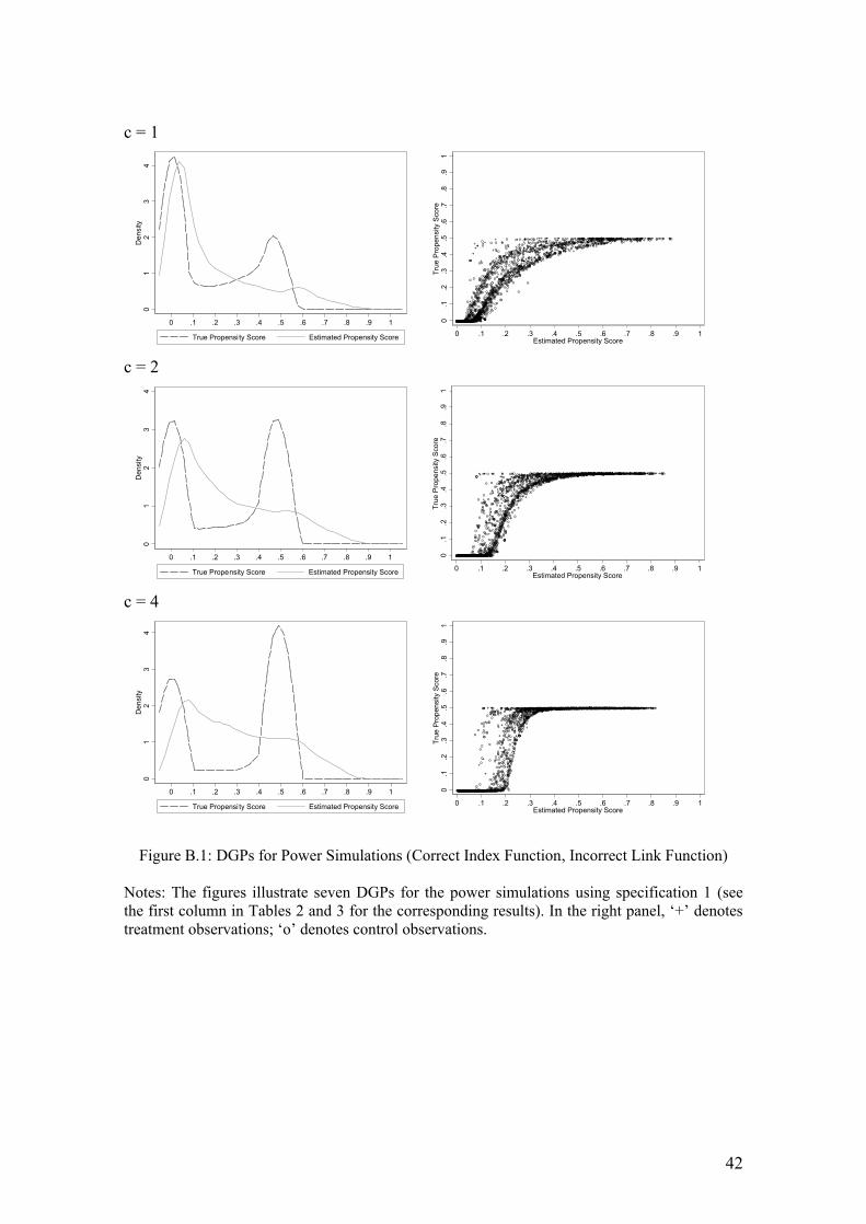
42

c = 1

01

23

4D

ensi

ty

0 .1 .2 .3 .4 .5 .6 .7 .8 .9 1


+ ooo+ o +o++o +++ oo +oo ++

+o o++ o oo ++o + o ++ o+o o ++o oo+ oo + oo+ + oo +oo+ oo ++ ++ ++ ++ ++o + ++ + ooo o +o+ ooo oo ooo o + ++ o+o + +ooo++o o++ ++ o+++o +oo +oo o

+

o o oo oo oo+ + ooo o+o +o o+ o +o oo ++ + +oo ++ o o++o++ oo oo ++o+

+++ o o++

+

o+

o

o

o

+o +

+

o

o

o

+

o

+o

o

o

+

o

o

o

o

+

+o

+

o

o

o

o

+o

o

+o+

o

oo

o

o

+

o

o

o

+o +

+

o+o

o

+

o

o+

++

o

o

o

+

o+

+oo

++

o

oo

ooo+

o

+

oo

o

o

o

o

o o

o

o

+o

o

o

o

o oo

+

o

o

oo+

+

o o

o

o

o

o

++

+

o

oo

o

o

ooo

ooo

o oo

o

o

o

o

o

o ooo

o oo oooo

o

+

++

o

+

+

o

o

oo

o+

o

+

+

ooo

+

++

+

o

+ o

+

++ o

o

o

o

oo

o+

o

o

+

oo

o

+ +

o

o +++

o

+

o

o

o

o

o+

+

o o

+

o

+

+

+

o

o

o+

oo

o o

o

+

o

o

o

o

o

oo ++

o

o

o ++

oo

+o+

++

o

++

o

ooo

o

o

+

o

+

+

o

o

+o +o +

++o+

+

o

o+

o

o

o o

+

+

o

+

o

o

o

oo

+

o

+

+

+

oo

+o

oo

o

o

o

+

o

++

o

++o

o

o

+

+

o

+oo

+o +o

+

+

o

o

++

o

+

+o

o

oo

o+

o

+

o+

o

o

+

o

+

o

o

oo

o

o

+

o

oo

+

o

+

++

o

o+

o+

o

o

+

o

o

o

o

+

o

o

o

+

o

o

+

o+

o

o

+

+

o

o

+

o

o o

o

+

+

o

+

+

oo

+

o

oo

o

o

oo+

o

o

+

o

o

o

o

+

o

o

o

o

+

+

+

o

oo

o

+

o

o

o

+

o

o

o

o

o

o+

+

o

o

o

+

ooo

o

o

oo

++

o

o

o

o

o

o

+

+

o

o

o

o

o

o

o

o

+o

o

oo

+

o

o+

+

o+o

o

o

+o

o+

o

o

oo

+o

o

o

o

oo

o

oo

+

o oo

+

o+

o

o+

+

o

o

o

o

o

o

+

o

o

o

o

+

o

o o

o

o

+

+

+

o

o

o

oo

oo

o

o

o

o

ooo o

+

o

o

+

o

o

oo

oo

+

o

o

o

+

o

o

o

o

+

o

o

o

o+

o+

o

++

o

o

o

o

o

o

oo

+

o

oo

o

o

oo

o

+

o

oo

o

+

o

o

+

o

ooo o

+

ooo ooo

o+

o

o

o

o

++

o

o

o

+

+

o

o

oo

o

+

o

+

+

o

o

o

o

oo

o

o

o

o

o

o

oooo

o

oo

+

o

oo

o

o

o

o o

o

oo

oo

o

o

o

o

o

oooo

o

oo

o

o

o

oo

oo

+

o

o

o

o

+

o o

o

oo

o

o

o

o

+

o+

o

o

o

o

oo

+

ooo

o

o

o

o

o

o

oo

o ooo

+

o

+

o

oo

oo

o

o

o

o

o

+

o oo

o

oo

o

o

o

o

+

+

o

oo

oo

o

o

+o

o

o

o

oo

o

o

o

o

o

oo

o

o

o

o

o

+o

o

o

+ o

o

+

+o

o

+

o

o

+

oo

o

o

++

oo

o

+oo

o

oo o

o

o

o

o

o

o o o

o

+

o

o

oooo

oooo

ooo

oo

ooo

oo

o

o

o

o o

++

oo o

o

oo

ooo

o

o

o

o

ooo o

o

o

o

+oo

o

+

o

oo

oooo

oo

oooo

o

oo

o

+

o

o o

o

o

o

ooo

+

ooo

o

oo oo

o

oo

o

oo

o

++

+

o+

+

oo

o

o oo oo

oo

ooooo

oooooo o oo o ooo oooo oo

o

ooo

o

oo

o

o o

+

o

o

o

o ooooooo o

o

oo

o

o

o

ooo oooo ooo

+

oooo o

o

ooooooo oo o

+

oo

+

+

o

+

o

oo

o

o

o

o

oo

ooo

o

o oo o+

+

o

o

o

o

o

o

oo

o

oooo oo

ooo oo o

o

ooo ooo ooooooo ooooooo o

o

oo oooooo oo

oo oo

o

oo

o

o

o

o oo o o

o

o

oo

o

o ooo

o

o ooo ooo

ooo ooo ooo o

o

o oooo oo

oooooo oooooo

o

+

o

o

+

o

o

o

o

o

o

ooo o

o

o oo

oo

oooooooooo oo o

o

o ooooooo

o

ooo

o

o

o

oo ooo o

o

ooo ooo ooooo oo

++

o

oo

o ooo

o

oooooo

+

o oo

o

oo

oo

o o oo ooooo oo ooooo oo ooooo ooooo ooooo o

o

ooo oooo oo oooo oooooo oooo

+

oo ooo

+

o

o

o

+

o o o

o+

o oo oo oooooo ooo ooo oo oooo ooooo ooo ooooooo ooo oo

o

oooo

oo ooooo oo oooo ooo ooo oo ooooooo ooooooooo o oooooooo oooooo oooooooooo oooo ooooo o oo ooooooooooo ooooo oo oo oo ooo ooo oo oooooooo ooo

o

o

o

o ooo

+

ooooo

o

ooo

oo

oo

ooooo ooooo ooooooooooooooo oooo o

+

oooooo

o

o

o

o

+

o ooooo oooooo oooooooo oooo

+

o

ooooooooooooo oooo oooooooooooo

o

o

oooooooo oo oooooooo o

+

o

o

o

oo

ooooooooo oooo oo ooooo oooooooo oooooooooooooooooooooooooooooooooooo oooooooo ooooooooooooooooooooo ooo

o

ooooo

+

oo

++

ooo

oo

+ o

+

o+o+

+

o

+ ++

o o

o

++

o

o o++

+

o

+o

o

+

+ o

o

oo+o

o

+

o

+

+o

o

o

o

oo

+

o

o

o

o

oo

+

o

+

++

+o+

+

oo

+

oo

+

oo

+

+

o

o

++

+

o +o o+

+o

o++o

+ +o ++ +

o

+ o

o

+o+

o

+

+

o

oo

o o+o+o

o +

+

+

+++

++

oo

+

o

+++

o

oo

o

o++

o

+

+o

+ o

o

+ +

+

ooo

o

o

+

+

o+

o

ooo

o

+ o

o

o

o

o

o++

oo

o

o

o

o

+++oo +

oo

++

+ oo

o+

o

+

o+

o

o

+o

+

oo

o oo

o

o+

o

oo++

oo

o

o

o

o+ + +o

o

o

oo

o+

o

o

o

+

o

o

+

+

++

+

+

o

+

o

o

o

+ +

oo

o

+

o

o+

o

o

+

+

o

+

o o+ o

o

oo

+oo

o

oo

o

oo

o

o

o

oo

o

o

+o

o

o+

oo ooo

++

o

+o

ooo

o o

o

o

o

o

o

o+

o

o

ooo

oo

o

o

o

+

oo

o

ooo

oo

o

oo

+oo

o

o

o

o

o

o

oo

+

+

o

oo

o

o

+

+

o

o+

o

+o

ooo

o

oo

o

o

o

oo

o

o

o

o

o

oo

o

ooo

+

o

oo

oo

+

o

+

o

o

oo

o

o

o

o

+

o

o

o

o

o

+

+

oo

o

oooo

oo

o o

o +

o

oooo

+ +o

oooo

+

o

o

+

+

o oo

+

ooo

o

o

oo

oo

o

+

+o

o

ooo

o

ooo

o

o

+

+

oo

o

o

o

o o+

o

o

+

+

o

ooo

+

o

o

oo

o

o

o

o

o

o

o

o

o

o

+

o

oo

+

o

oo

oo

o

o

+

o

o

o

+

oo

o

+

o

oo o

o

o

o

+

++o

+

o

o

oo

o

o

o

o

oo

o

o

o

o

o

o

o+

oo oo

o

o

o

o

+

oooooo

o oo

o

o

o oooo

o

o

o

ooo

o

o

o

o

oo ooo

o

oo

oooo

oo

o

+

o

o o

o

o oooo

o+

o oooo

oooo oo

o oo

o

oo

oooo

o

oo oo

o

+

oo

oo

oooo

o

o

ooooo oo

o

o

ooo ooo

o oo

oooooo oooo

o

o

+

oooooo

o

o

+

oooo

o

oo

o

o

o

oo o

+

o oooooooooooooooo

o

ooo oooooooooo oooo

oo

oo ooooooo

o

o oooooo0.1

.2.3

.4.5

.6.7

.8.9

1Tr

ue P

rope

nsity

Sco

re


c = 2

01

23

4D

ensi

ty

0 .1 .2 .3 .4 .5 .6 .7 .8 .9 1

True Propensity Score Estimated Propensity Score

+ ooo +o +o+ +o+++oo +oo +++ ooo+ o oo ++o + o ++ o +o o + +o oo+ oo + oo++ oo+ oo+ oo ++ ++ ++ ++ + +o + ++ +ooo o +o +o oo oo oooo + ++ o+o + +ooo+ +o o+ + ++ o ++ +o +oo +oo o+o o oo oo oo+ + oo o o +o +o o+ o +o oo ++ + + oo ++ o o+++++ oo o o ++o ++++ o o+ + +o+oo

+

+o + +

o

oo

+o+ o

+

o

+o

o

+

o

+ +o +o

o

o

o

+o + +o+

o

oo

oo +

o

o

o

+ o ++o++

+

+o o+++

oo

o+

+++oo + + o

+o

ooo+

o

+

oo

+

o

o

o

o o

o

o

+oo

+

+

ooo

+

o

o

oo++ o oo

oo

o

++ +

o

ooo

+

ooo

o+o

o oo

o

o

o

o

o

o o

+o

o oo oooo

o

+ +++ +

+

oo

oo

o+o + +

ooo

++ + +

o

+ o+ ++ o

+

o

o

o oo+

o

o + o+

o

+ +o

o +++

++

o

o

o

o

o++

o

o

+

o

+++

o

o

o+ +o o o

o

+

o

o

+

o

o

oo ++o

o

o ++oo

+o + ++

o

++

o

+oo

o

o

+

o

++

o

o

++ +o ++ +o+ ++ o+oo

o

o

++o

+ oo

o

o o +o++ +oo

+o oo

o

o

o

+

o

++

o

++oo

o

+ +

o

+oo+ o +o

++

+

o+ +o

++o

oo+

++

o

+

o+

o

o+

o

+o

+

o oo

o

++

oo

+o

++++

o +

o +

+

o +

+

+

o

o+

o

o

o

+

+

o

+o +oo

++

o

o

+o o o++ +

o

++

o o+

+

oo

o

o+o+

oo

+

+

o

o

o

+o

o

o

o

+

+

+

o

oo

o

+

o

o

o

+

o

o

o

o

o

o+

+

o

o

o

+

oo

o

o

o

o

o

+ ++

o

+o

o

++

+

o

oo

o

oo

o

o

+o

o

oo+

o

o++ o+ o

o

o

+ oo+

o

o

oo

+o

o

+

o

o +

+

oo

+

oo

o

+

o+

o o+

+o

o

o

o

o

o

+

o

o

o

o

+

+

o o

o

o

++

+

o

o

o

o+

oo

o

o

oo

ooo o

+ oo+

o

o

oo

oo

+

o

o

o+

+o

o

o

+

+

o

o

o+

o+o

++o

o

o

+

o

o

oo

+

o

oo

o

o

oo

o+

o

+ o

o

+

o

o+

o

oo

+

o

+

ooo oo o

o+

o

o

o

o

++

o

+

o

+

+

o

o

o

o

o

+

o

+

+o

o

o

o

oo

oo o

o

o

o

oo

oo

+

o

o

+

o

o

o

o

o

o

oo

o +o

oo

o

o

o

o

o

oooo

o

o

o

o

+

o

o

o

oo +

oo

+

o+

o o

o

o

+

o

o

o

o

+

o+

o

o

o

o

+

o

+

ooo

o

oo

o+

o

o

o

o ooo

+

o

+

+o

o

o

o

o

o

+

o

o+

o

o

o

o

oo

+

o

o

o++

+

oo

++

o

o

+oo

o

o

o

o

o

o

o

o

o

+o

o

o

o

o

o

+o

o

o

+ o

o

+ +oo ++

o

+

o

o

o

o

+ +

oo

o

+ +o

o

+o +

o

+

o

o

o

o o o

o

+

+

o

+

ooo

oo

o+

o

o

+

o

o

ooo

o+

+

o

o

o o

+ +

o

o

+

o

oo

o

oo

o

+

o

+

ooo o

o

o

o

+o

o

o +

o

o

o

oooo

+o

ooo o

o

oo

o

+o

o

o

o

o

o

ooo

+

ooo

+

oo

o

o

o+

+

+

o+

+

++

+

o+

+

oo

o

o

o

o oo

oo

o

oo

o

o

o

o

o

ooo o ooo

+

oo oooo oo

o

o

o

o

o

o

o

o

o

o

+

o

o

+

oo

ooooo o o

o

oo

+

o

o

o

oo

+oo

o oo

o

+

oo oo o

o

+o

o

oooo

o

o

o

+

o

o

++

+

+

o

+ o

o

o

+

o

++

o

oo

o

o oo o

+

+

o

+

o

o

o

o

oo

o

oooo o

o

ooo oo

o

+

oooo

oo

ooooooo oo ooooo o

o

oo ooooooo

+

oo oo

o

oo

+

o

o

o oo o o

+

o

o

+

o

o oo

o

o

oo

oooo

o

ooo o oo ooo o

o

o oooo o

o

o ooooo

+

oo

ooo

+

+

o

o

+

o

o

o

o

o

o

oo

o

+

+

o oo

o+

ooooo o oo oo oo o

+

o oooooo

+

o

ooo

o

oo

oo ooo o

o

ooo ooo o ooo o oo

++

o

o

o

o

o

oo

o

oooooo

+

o oo

o

o

o

o

o

o o +

o o+

ooo oo ooooo oo

+

oooo o oooo

o

o+

oo o

+

o oo oo oo oo ooooo

ooo oo ooo o

+

oo ooo

+

o

o

o

+

o o o

o+

o

o

oo

oo

oo ooo ooo ooo oo

o

oo o ooooo ooo o ooooo o ooo oo

o

ooo

o

o

o o

o

ooo oooooo ooo o

o

o oo ooooo o oo

oo oooooo o oooooooo ooo o oo ooo ooo oooo oooo ooooo o

o

o ooo oooo oo oo ooooo oo oo oo ooo ooo oo ooo ooooo ooo

o

o

o

o ooo

+

o oo oo

o

o oo

o

+

++

ooooo oo ooo ooo oooooooooo oo oo oo o

+

oooo oo

o

o

o

o

+

o ooooo ooo ooo ooooooo o oooo

+

o

oooo ooo oo oo oo

oooo oo ooooo ooooo

o

+

ooo ooooo oo oo oooooo o

+

o

o

o

oo

oo ooooooo

o

oo o oo oo ooo ooooooooo

ooooooooooooooooo ooo o ooo oooo oo oooooo

ooooo oo ooooooooooooo oo ooo ooo

o

oo

o

ooooo

+

oo

++ooo o o + o

+

o+ o++

+

+ ++o +o

++

o

o o++ +o +o

+

+ + oo

oo+o

+

+

o

++ + o

+

+

oo

+

oo

o

+

o o+

o

+

+ ++o+ +

oo

+

oo

+

oo

++

o

+ +++ o +o o+ +oo++o + +o++ +

o

+ o

o

+o+

o

++ oooo + +o+oo + +++++++o o

+

o

+ ++o

o

o

o o++

o

+ +o+ oo + ++ oo o

o

o ++ o +

o

ooo

o

+ o+ oo

o

o ++ oo

o

ooo +++ oo +

o+

+ ++ o o++

o

+o+o

o+o

+

ooo o o

+

o+o

oo ++ooo

+

+

o + ++o

o

o

o

o

o+oo

o

++

o

++

+++

++ +

o

o

o

+ +o+o+

oo+

o

o ++

o

+o o+ o

+

oo

+oo

o

ooooo

o

o

ooo

oo

+oo

++

o+ oo o+ +o

+o

o

oo

o o

o

o

+

oo

o+o

o

o o

o

oo

o

o

o

+

o

o

o

o

oo

o+

+oo+oo

o

o

o+

+

+

o++ +o

o+o

o

+ +oo+o++

o

oo

ooo

o

oo

o

o

o

o

o

o o

oo

o

ooo

++

oo

oo

+

o

+

o

o

o o

oo

o

o

+

o

+o

o

o

+

+

o o

o

oooo

oo

o +

o ++

oo oo++o

oo

oo

+o

o

+

+

o

o

o

+

ooo

o

+

oo

oo

o

+

+o

o

+oo

o

o

oo

+

o

+

+o o

o

o

oo o+

+

o

+ +o

ooo+

o+

ooo

+

o

o

o

+

o

o

o

o

+

o

o

o

+

o

oo

o

o

+

o

+

+

o

o

+

oo

o+

o

oo o

o

+

o

+ + +o+

o

o

oo

o

o

o

o

+o

o

o

+

o

o

o

o+

o o oo

+

o

+

o

+

o

o

oo oo

o oo

+

o

o

oo

o

+

o

oo

o

oo

o

o

o

o

oo ooo

o

o+

ooo o

+o

o

+

o

o +

+

ooooo

o+

o oo

+o

ooooo

o

o

o

o

+

o

o

oooo

+

o

o

o

o

o

+

oo

o

o

o

oo

o

+o

oo ooo oo

o

o

ooo oo

o

o

o

o

ooo ooo oooo

o

o

+

o o oo oo

+

o

+

oo oo

o

oo

o

o

o

+

o o

+

o oooooooooooo oooo

o

oo oo

oo oo ooooo oooo

oo

oo ooooooo

o

o ooooo o0.1

.2.3

.4.5

.6.7

.8.9

1Tr

ue P

rope

nsity

Sco

re


c = 4

01

23

4D

ensi

ty

0 .1 .2 .3 .4 .5 .6 .7 .8 .9 1


+ ooo +o +o+ +o+ + +oo +oo +++ ooo+o oo ++o + o ++ o +o o + +o oo +oo + oo++ oo+oo+ oo ++ ++ ++ ++ + +o + ++ +ooo o +o +o oo oo oooo + ++ o+o + +ooo++o o++ ++o ++ +o +oo +o o o +oo oo oo oo+ + oo o o+o +o o+ o+o oo ++ + +oo ++ o o+++ ++ oo o o ++o ++ ++ o o+ + +o+ oo+ +o + +

o

o o +++ o+

o

+oo+

o

+ +o +o

o

oo +o + +o+o ooo o +

oo

o+ o++o+++ +o o+++o +o + +++oo+ + o

+o

ooo+

+

+

oo

++

o

o

oo

o

o

+oo+ +

o

oo

+

oo oo++ o oo oo

o

++ +o oo o+

ooo

o+o

oo

o

oo o

o

o

o o

++

o oo oooo

o + +++ ++

oo

oo

o+o + +

ooo

++ + +

+

+ o+ ++ o+

o

o

o o o+

o

o+ o+

o

+ +o o ++++ +o oo

o

++ +

o

o

+

o

+ ++

o

oo+ +o o o

o

+ o

o

+oo oo ++o

oo ++oo +o + ++

o

++o+ o +

o

o

+o ++

o

o ++ + o ++ +o+ ++ o+oo

o

o

+ +o+ oo

o

o o +o + + +oo +o oo+o

o

+o ++

o

++o+

o

+ ++

+oo+ o + o+ ++ o+ +o ++o oo+ ++o + o+o

o +o +o

+

o oo

o

++

oo

+ o ++++ o+o ++ o ++ +

o

o +o

o

o

++ + + o +oo++o

+

+o oo++ +

o

+ +oo++ oo

o

o +o+ oo ++

o

o

o

+o

o

o

+

+

+

+o oo o+

o

o

o

+

+

o

o

o

o

o+ +o

oo+

o+

o

o

+

o

o

+ ++

o

+ o

o

+ ++

o

ooo o oo

o

+ oo oo +o o++ o+ o

o

o

+ oo+ o

o

oo+oo

+ oo++

oo

+

o

o

o

+o + o o++ o

o

oo

o

+

+o

o+

o

++

o o

o

+

++ +o o oo+o o

o

o oo

ooo o

+ oo+

o

o

oo

o o +

o

oo ++o

o

o ++

o o o+o+o ++o o

o

+o

+

oo

+o

oo

+

o

o

o

o++

+oo

+

o

o +o

oo

+

+

+

ooo oo o

o+

o

o

o

o ++

+

+

o

++o

o

o

o

o+o

+ +o

o

oo

oo

o o oo

o

o

o

+

oo

+

o

o

+ o

o+

o

oo

o

o

o +o o++

o

o+

+

oo oo

o

o

o

o+ o

o

+

oo +o o+ o+

o

o

o

o

+

o

o

oo

+o+

o

o

+

o

+

+

+

ooo

oo o o+ooo

o ooo

+

o

++oo

o

o

o

o +

o

o+

o

+

o

o

oo

++

o

o+ ++

oo

+++

o

+o o

o

o

+

o

o

+

o

o

o

+

o

o

o

o

o

o +o

o

o

+ o

o

+ +oo ++

o

+

o

o

o

o

+ ++o

o

+ +o

o

++ +

o

+o o

o

o o

o

o

+

+

o

+

ooo

oo

o+

+

o

+

o

o

ooo

o++

o

o

o

o

+ +

+

o+

o

oo

o

+o

o+

o

+

o

oo o

o

o

++o

o

o +o

o

o

o

ooo

++

ooo o

o

o o

++o

o

o

o

+

o

+

oo

+

o

o+

+

oo

+

o

+ ++

+

o++ +++o+ +

oo

o

o

o

o oo

++

+

oo

+

o

o

o

o

ooo o oo

o

+

o

ooo

oo oo

o

o

o

o

o

o

o

+

o

o

+o

o

+

o

o

ooooo o o

o

oo

+

o

o

o

o o

+o

+

o o

o

o

+

o ooo o

o

+oo

oooo

o

o

+

+

o

o

+++ +

o

+ ooo

+

+++

o

oo

o

o oo

o

+

+

o

+

o

o

o

o

oo

o

o

ooo o

o

o

oo oo

o

+

ooo

o

oo

o

o

oo

ooo oo ooooo o

o

oo

+

ooo o o

o

+

o

o

o

o

o

o

o

+

o

o

o

o

o o

o

+ o

o

+

o

o

o

o

o

o

o

o

oo

oo

o

ooo ooo ooo o

+

o ooooo

o

o o oooo

+

o

+

ooo

++

o

o

+

+

oo

o

o+

oo

o

+

+

o oo

o+

+

oooo o oo oo oo

o

+

o oooooo

+

o

ooo

o o+

oo ooo

o

o

ooo

o

oo o oooo

o

o

++

o

o

o

o

o

o o

o

oooooo

+

o oo

o

+

o

o

o

o o+

o o

+

ooo oo

o

+

ooo

o

o

+

oooo o oooo

o

o

+

oo o

+

o oo

o

o oo oo oooo

o

ooo oo o oo o

+

oo ooo

+

o

o

o

+

o o o

o+

o

+

o

o

o

o

oo ooo oooo

oo oo

o

oo o ooooo ooo o oooooo ooo

o

o

o

ooo

o

o

o o

o

ooo oo

o+

oo ooo

o

+

oo

oooooo o o

o

oo oooooo o oooo oooo ooo o oo ooo o oo oooo oooo oo oo o o

o

o ooo oo oo oo oo ooooo oo oo oo ooo ooo oo ooo ooo oo ooo

o

o

o

o ooo

+

o oo oo

o

o oo

++++

oo

ooo oo ooo ooo oooooooo oo oo oo oo o

+

oooo oo

o

o

o

+

+

o oo oooo

oo ooo ooooo oo o ooo o

+o

o

ooo ooo oo oo o o

o

o o o oo ooooo oooo o

o+

ooo oo ooo oo oo oooooo o

+

o

o

o

oo

oo oooooo o

o

oo o oo oo ooo ooo ooooo

o

oooooo oo oooo ooooo ooo o ooo oooo oo ooooo

o

ooooo oo ooooo oooooooo oo ooo ooo

o

oo

o

ooooo

+

oo

++ooo o o + o+

o+ o ++

+

+ ++o +o ++o

o o++ +o+o+ + + oo oo+o+

+ + ++ + o+ + oo+o o o+ o o+o

+ + ++o+ +oo +

oo

+

oo

++

+

+ +++ o +o o+ +oo++o + +o++ +

o

+ o

o

+o+

o

++ oooo + +o+oo+ +++++ ++ o o+o+ + +o

o

o

o o++o

+ +o+ oo + ++ oo o

o

o ++ o +

o

ooo

+

+o+ oo

o

o ++ ooo o oo +++ oo +o+

+ ++ oo++

o

+o+o o+o+ ooo o o+

o+o oo ++ooo

+

+o +++o

o

o

o

o

++ ooo ++o ++ +++ +++

o

o

o

+ +o +o +o++o o ++

o

+o o+ o+

oo

+ooo oooooo

o

o oo+o +oo+ + o+ oo o+ +o+o

o

+o

o oo o+ o oo+ o

o

o o

o

+ oo

o

o

+

o

+

o

o

oo

o+

+ oo+ooo

o

o++ + o+ + +oo +o+ + +oo+ o++

o

o+

oo o

o

oo

o

oo

+

o

oo

++

o

ooo

++oo

oo

+

o

+

o

o

o oo o o

o

+ o + o+o ++

o o

o

o ooo

ooo + o++ oo oo++o

o

o

oo

+o

o

+ +

o

+

o

+

o oo

o+

o

o

oo+ ++o

+

+o++

o

oo

+

o

++o o o

o

o o o ++

o

+ +o ooo+ o++o o+

o

o

o

+ o

o

o

+

+

o

o

o

+

o

oo

+

++

o

+

+

+

o

+

oo

o+o

oo o

+ +

o

+ ++o+o o

oo

o

o

+

o

+o+

o

+

o

o

o

o+

o ooo

+

o

+

o

+

o

+

o

o oo

oo++ o

o

oo

o

+

o oo

o

oo

+

o

o

o

oo ooo

o+ +

ooo o

+o

o

+o o++

o

oo+

o

o +

o

o

o

+o

oooo

o

+

o

+

o

+

+

o

ooo o

+

+

o

o

o

o +oo

+

o

o

oo

o

+ o

oo ooo oo

o o

o oo oo

o

o

o

o

ooo ooo oooo

o

o

+

o o ooo

o

+o

+

oo oo

o

o

o

o

o

o

+

o

o

+

o

+

oo ooooooooo oooo

o

oo o

o

oo oo ooooo oooo

oo

oo

oo

ooooo

o

o ooooo o0.1

.2.3

.4.5

.6.7

.8.9

1Tr

ue P

rope

nsity

Sco

re


Figure B.1: DGPs for Power Simulations (Correct Index Function, Incorrect Link Function) Notes: The figures illustrate seven DGPs for the power simulations using specification 1 (see the first column in Tables 2 and 3 for the corresponding results). In the right panel, ‘+’ denotes treatment observations; ‘o’ denotes control observations.

Documents

On Assessing the Specification of Propensity Score Models