On Appropriate Assumptions to Mine Data Streams: Analyses and

Solutions

Jing Gao† Wei Fan‡ Jiawei Han†

†University of Illinois at Urbana-Champaign‡IBM T. J. Watson Research Center

Introduction (1)

• Data Stream– Continuously arriving

data flow– Applications: network

traffic, credit card transaction flow, phone calling records, etc.

10

11

10

1

00

11

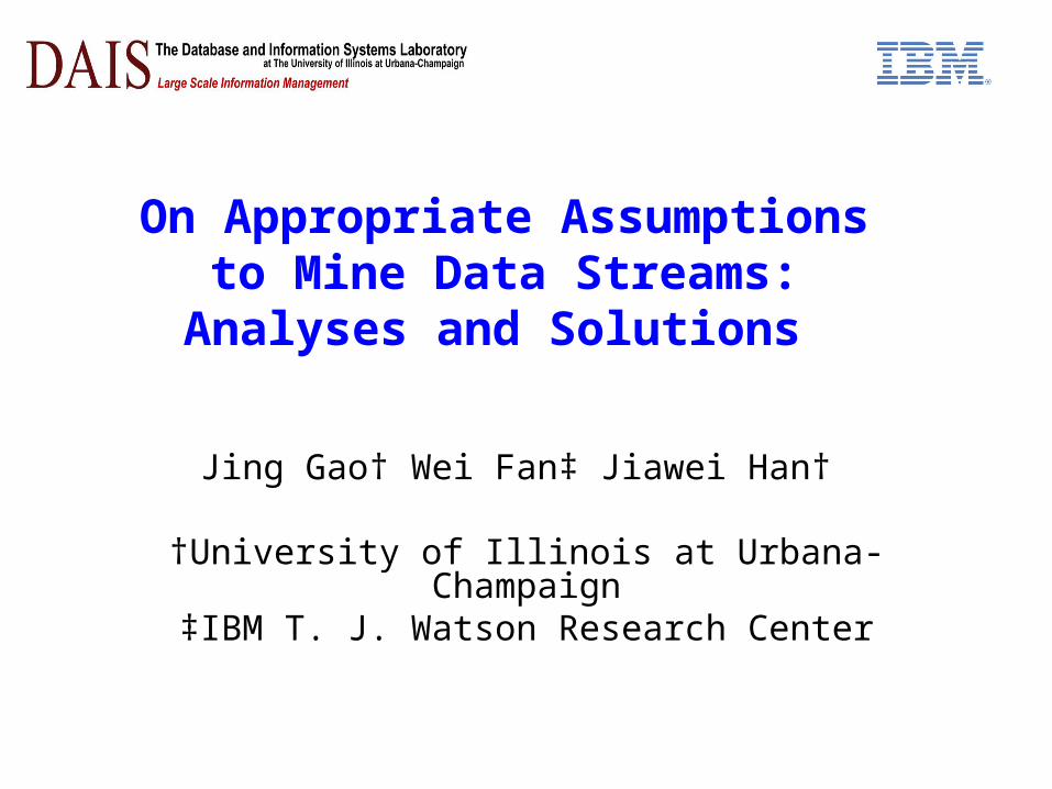
Introduction (2)• Stream Classification

– Construct a classification model based on past records

– Use the model to predict labels for new data– Help decision making

Fraud?

Fraud

Classification model

Labeling

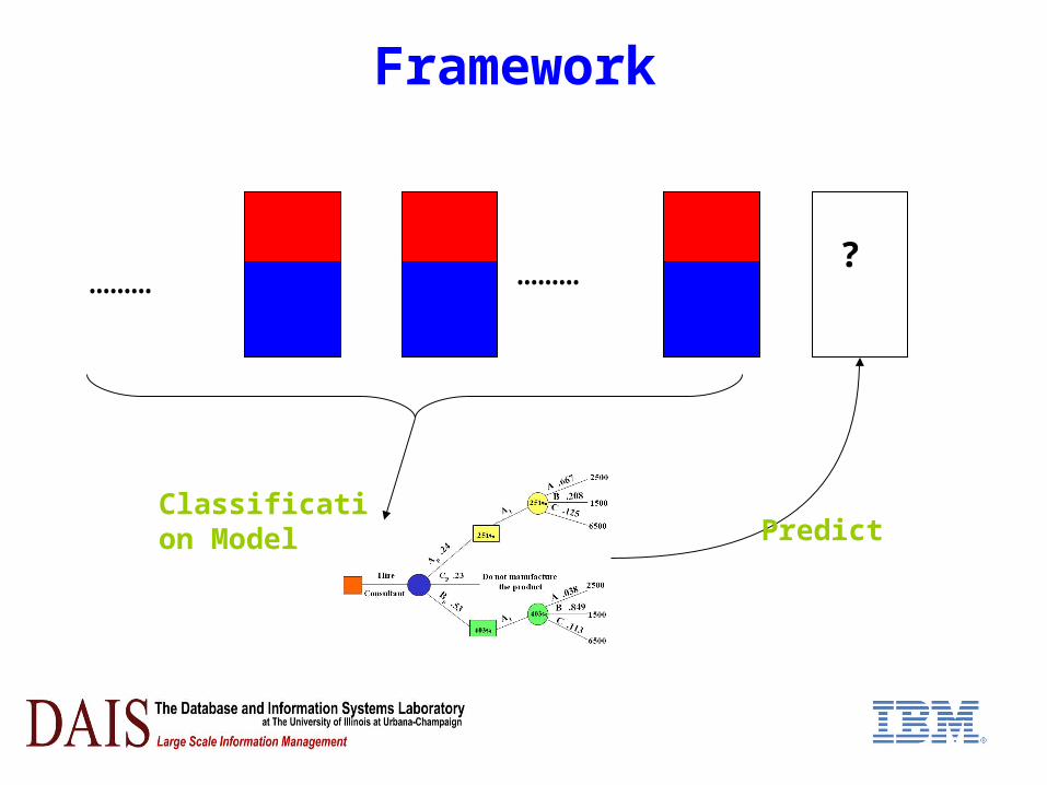
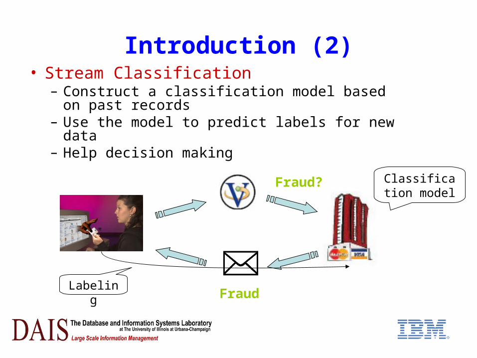
Framework

……… ?………

Classification Model Predict

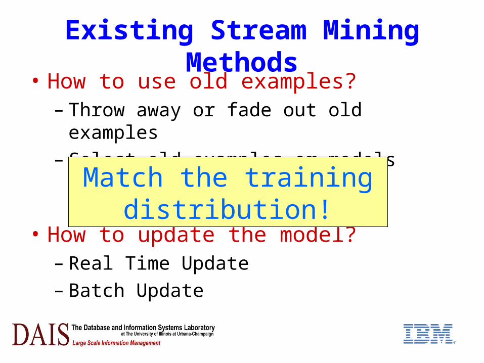
Existing Stream Mining Methods• How to use old examples?

– Throw away or fade out old examples – Select old examples or models which

match the current concepts

• How to update the model?– Real Time Update– Batch Update

Match the training distribution!

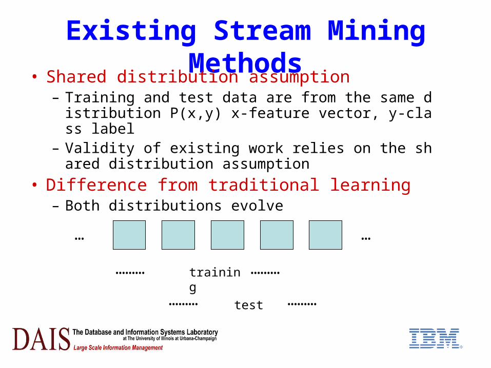
Existing Stream Mining Methods• Shared distribution assumption

– Training and test data are from the same distribution P(x,y) x-feature vector, y-class label

– Validity of existing work relies on the shared distribution assumption

• Difference from traditional learning– Both distributions evolve

……… training ………

……… test ………

… …

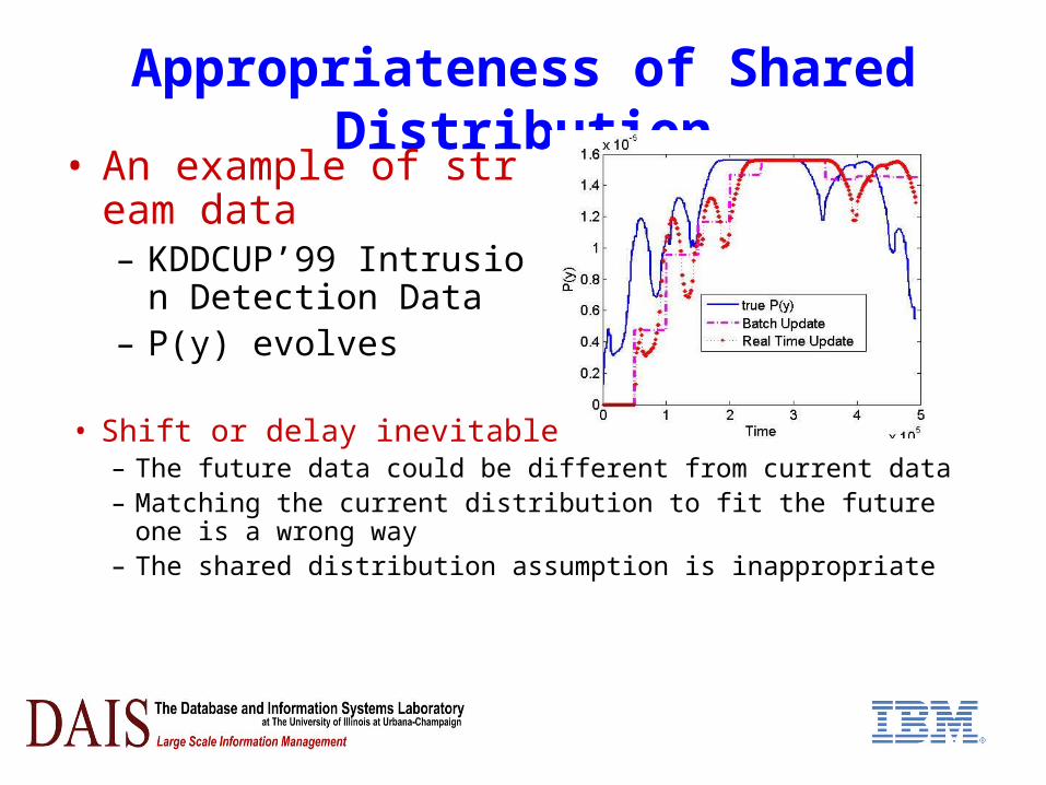
Appropriateness of Shared Distribution• An example of stream

data– KDDCUP’99 Intrusion D

etection Data– P(y) evolves

• Shift or delay inevitable– The future data could be different from current data– Matching the current distribution to fit the future one

is a wrong way– The shared distribution assumption is inappropriate

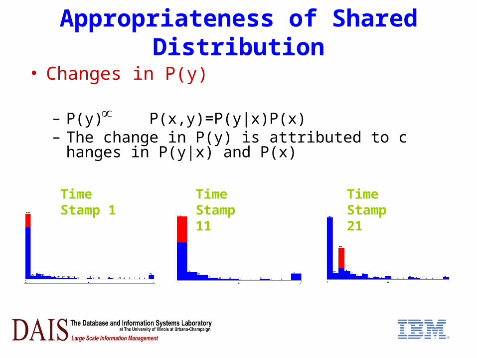
Appropriateness of Shared Distribution

• Changes in P(y)

– P(y) P(x,y)=P(y|x)P(x) – The change in P(y) is attributed to changes in P

(y|x) and P(x)

Time Stamp 1

Time Stamp 11

Time Stamp 21

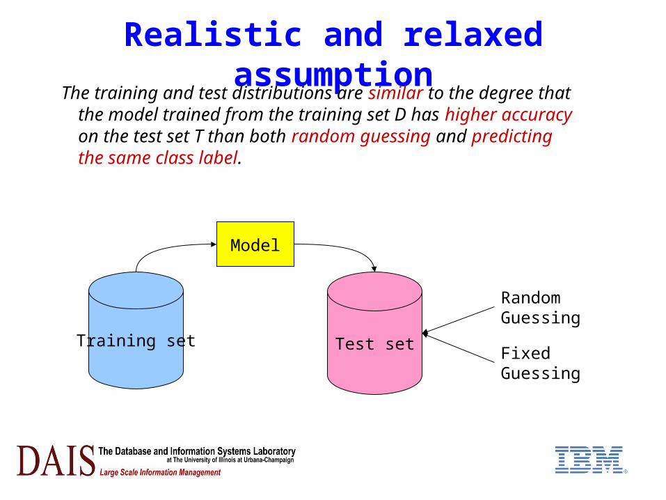
Realistic and relaxed assumptionThe training and test distributions are similar to the degree that

the model trained from the training set D has higher accuracy on the test set T than both random guessing and predicting the same class label.

Training set Test set

Model

Random Guessing

Fixed Guessing

Realistic and relaxed assumption

• Strengths of this assumption– Does not assume any exact relationship

between training and test distribution– Simply assume that learning is useful

• Develop algorithms based on this assumption– Maximize the chance for models to succeed on

future data instead of match current data

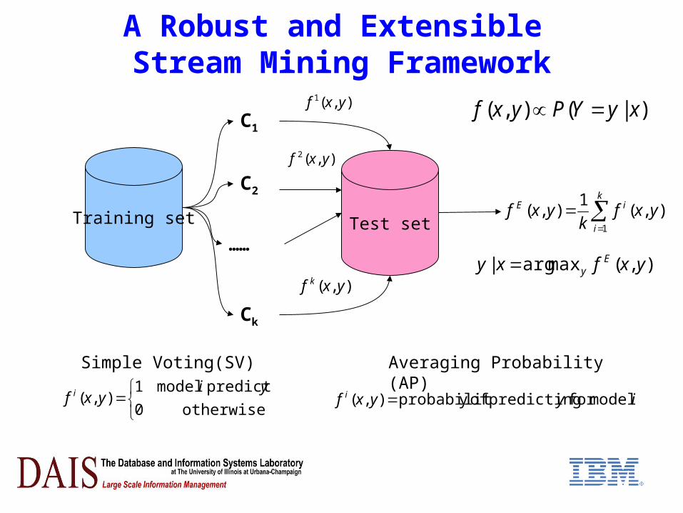
A Robust and Extensible Stream Mining Framework

),( yxf k

k

i

iE yxfk

yxf1

),(1

),(

),(2 yxf

C1

C2

Ck

……

Training set Test set

),(1 yxf )|(),( xyYPyxf

),(maxarg| yxfxy Ey

Simple Voting(SV) Averaging Probability(AP)

otherwise0

predictsmodel1),(

yiyxf i iyyxf i modelforpredictingofyprobabilit),(

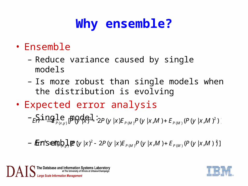
Why ensemble?

• Ensemble– Reduce variance caused by single models– Is more robust than single models when the

distribution is evolving

• Expected error analysis– Single model:

– Ensemble: )]),|((),|()|(2)|([ 2

)()(2

),( MxyPEMxyPExyPxyPEErr MPMPyxPS

])),|((),|()|(2)|([ 2)()(

2),( MxyPEMxyPExyPxyPEErr MPMPyxP

A

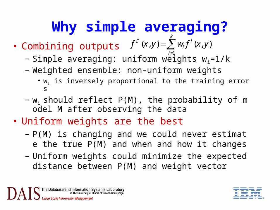
Why simple averaging?• Combining outputs

– Simple averaging: uniform weights wi=1/k– Weighted ensemble: non-uniform weights

• wi is inversely proportional to the training errors

– wi should reflect P(M), the probability of model M after observing the data

• Uniform weights are the best– P(M) is changing and we could never estimate the tru

e P(M) and when and how it changes– Uniform weights could minimize the expected distanc

e between P(M) and weight vector

k

i

ii

E yxfwyxf1

),(),(

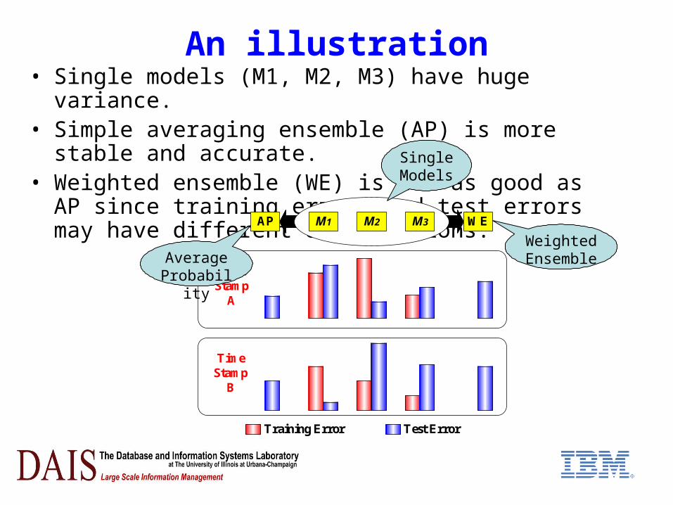
An illustration• Single models (M1, M2, M3) have huge variance.• Simple averaging ensemble (AP) is more stable and

accurate.• Weighted ensemble (WE) is not as good as AP since

training errors and test errors may have different distributions.

M1 M2 M3 WEAP

Time Stamp

A

Time Stamp

B

Training Error Test Error

Average Probability

Weighted Ensemble

Single Models

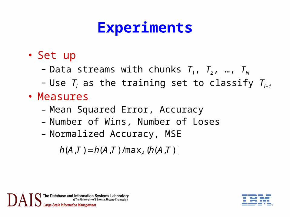
Experiments

• Set up– Data streams with chunks T1, T2, …, TN

– Use Ti as the training set to classify Ti+1

• Measures– Mean Squared Error, Accuracy– Number of Wins, Number of Loses– Normalized Accuracy, MSE

)),((max/),(),( TAhTAhTAh A

Experiments

• Methods– Single models: Decision tree (DT), SVM, Logistic

Regression (LR)– Weighted ensemble: weights reflect the accuracy on

training set (WE)– Simple ensemble: voting (SV) or probability

averaging (AP)

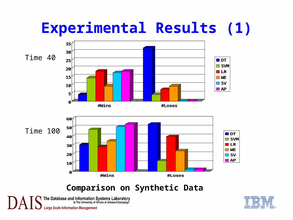
Experimental Results (1)

0

5

10

15

20

25

30

35

#Wins #Loses

DTSVMLRWESVAP

Comparison on Synthetic Data

0

10

20

30

40

50

60

#Wins #Loses

DTSVMLRWESVAP

Time 40

Time 100

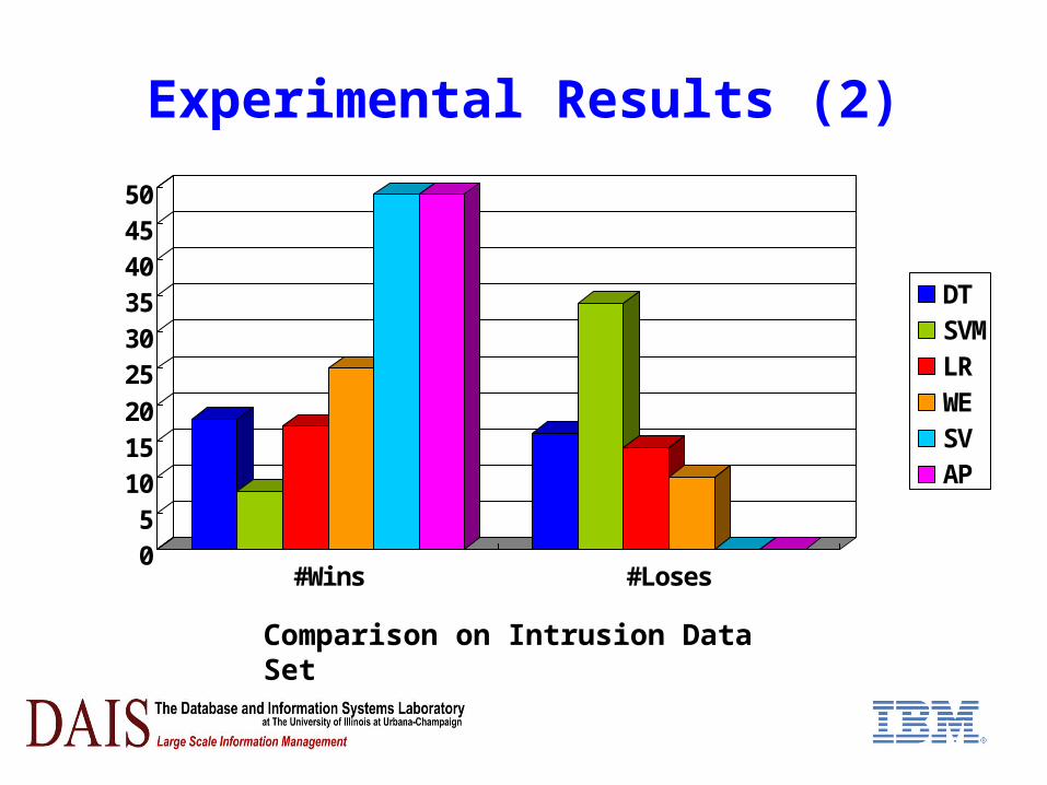
Experimental Results (2)

Comparison on Intrusion Data Set

05101520253035404550

#Wins #Loses

DTSVMLRWESVAP

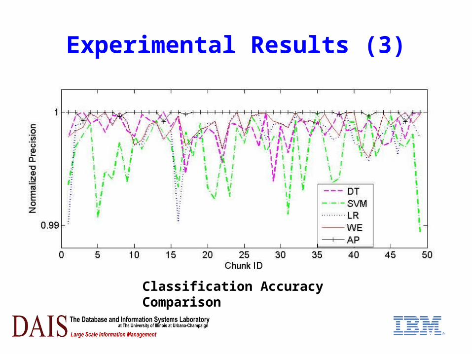
Experimental Results (3)

Classification Accuracy Comparison

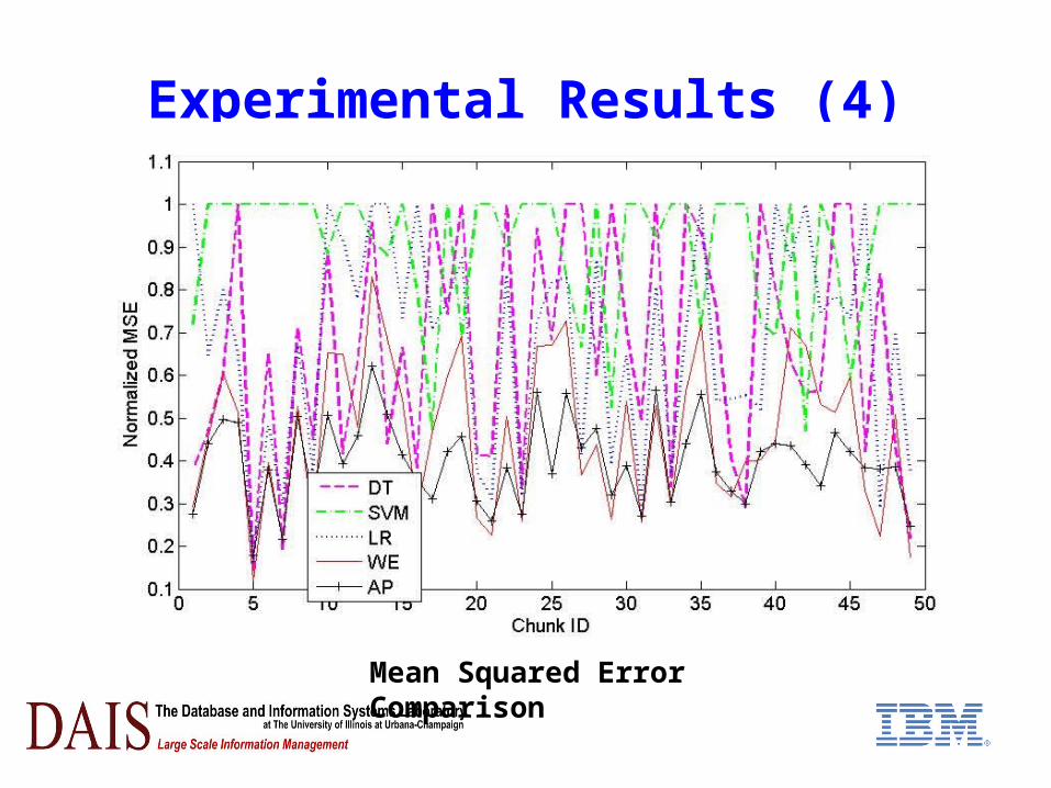
Experimental Results (4)

Mean Squared Error Comparison

Conclusions

• Realistic assumption – Take into account the difference between

training and test distributions– Overly matching the training distribution is

thus unsatisfactory

• Model averaging– Robust and accurate– Theoretically proved the effectiveness– Could give the best predictions on average

Thanks!

• Any questions?