Embed Size (px)
Citation preview
5/20/041
On Analytical Tools for Market Basket (Associations) Analysis.By Leonardo E. Auslender
SAS Institute, Research & DevelopmentLeonardo dot Auslender �AT� sas dot com
Presented at NYC Informs, New York City, NY, May 2004
5/20/042
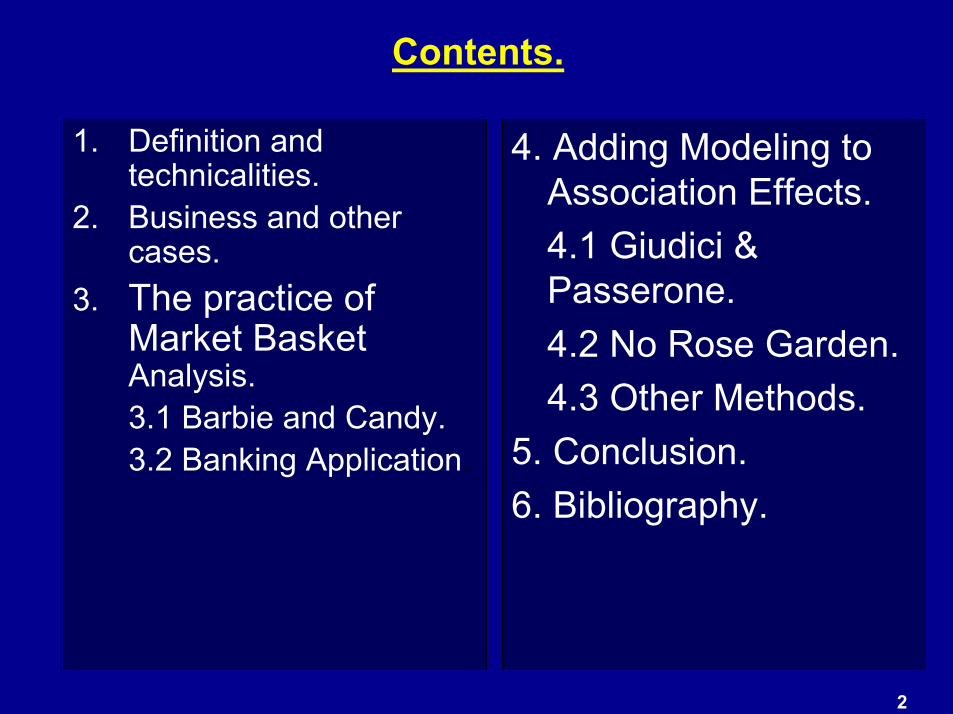
1. Definition and technicalities.
2. Business and other cases.
3. The practice of Market BasketAnalysis.3.1 Barbie and Candy.3.2 Banking Application.
4. Adding Modeling to Association Effects.4.1 Giudici & Passerone.4.2 No Rose Garden. 4.3 Other Methods.
5. Conclusion.6. Bibliography.
Contents.
5/20/043
5/20/044
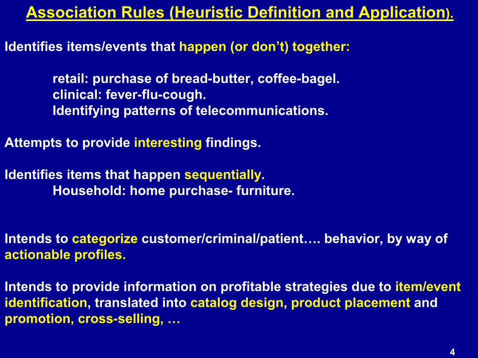
Identifies items/events that happen (or don�t) together:
retail: purchase of bread-butter, coffee-bagel.clinical: fever-flu-cough. Identifying patterns of telecommunications.
Attempts to provide interesting findings.
Identifies items that happen sequentially.Household: home purchase- furniture.
Intends to categorize customer/criminal/patient�. behavior, by way of actionable profiles.
Intends to provide information on profitable strategies due to item/eventidentification, translated into catalog design, product placement and promotion, cross-selling, �
Association Rules (Heuristic Definition and Application).
5/20/045
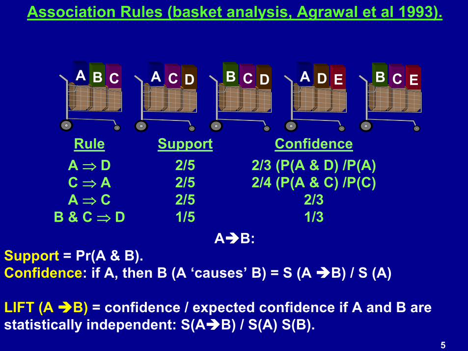
Association Rules (basket analysis, Agrawal et al 1993).
RuleA ���� DC ���� AA ���� C
B & C ���� D
Support2/52/52/51/5
Confidence2/3 (P(A & D) /P(A)2/4 (P(A & C) /P(C)
2/31/3
A B C A C D B C D A D E B C E
A����B: Support = Pr(A & B). Confidence: if A, then B (A �causes� B) = S (A ����B) / S (A)
LIFT (A ����B) = confidence / expected confidence if A and B are statistically independent: S(A����B) / S(A) S(B).

5/20/046
Association Rules: Implication?Checking Account
S(CK) = 85%, S(SVG) = 60%.S(SVG ����CK) = 50%C(SVG ���� CK)= .5 / .6 = .83 (also 5000 / 6000)Lift (SVG����CK) = .50 / (.85 * .6) = .83 / .85 = .98, CORR = -0.05Lift(SVG����~CK) = .10 / (.15 * .6) = 1.11
Lift > 1 ���� �positively correlated� and vice-versa. THESE ARE THE RULES TO LOOK AT.
500 3,500
1,000 5,000
No
Yes
No Yes
SavingAccount
4,000
6,000
10,0008,5001,500
5/20/047
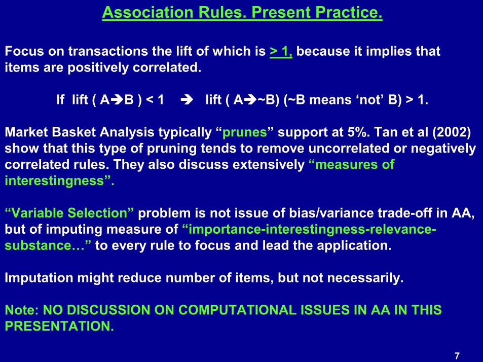
Association Rules. Present Practice.
Focus on transactions the lift of which is > 1, because it implies that items are positively correlated.
If lift ( A����B ) < 1 ���� lift ( A����~B) (~B means �not� B) > 1.
Market Basket Analysis typically �prunes� support at 5%. Tan et al (2002) show that this type of pruning tends to remove uncorrelated or negatively correlated rules. They also discuss extensively �measures of interestingness�.
�Variable Selection� problem is not issue of bias/variance trade-off in AA, but of imputing measure of �importance-interestingness-relevance-substance�� to every rule to focus and lead the application.
Imputation might reduce number of items, but not necessarily.
Note: NO DISCUSSION ON COMPUTATIONAL ISSUES IN AA IN THIS PRESENTATION.

5/20/048
( SAS EM Association Node (clipped) set of rules below).
Number of rules �discovered� (reported in descending order of support) is usually large, what is relevant and interesting and what is merely anecdotal?

5/20/049
For (mostly SAS) programmers only.
How could I program this if I just wanted to?
Go Proc Summary and IML, with good macro doses. Make sure you understand the _type_ variable before you start.
5/20/0410

5/20/0411
Association Rules (basket analysis by example).
Young-family high-income professional bank customers, two groups: high- and low-profit.
Mutual funds, mortgagescredit cards
Mutual funds, credit cards. SUREACTION:
Sell mortgages to this Group?

5/20/0412
Association Rules (basket analysis by example).
Mutual funds, credit cards. SURE ACTION:
Sell mortgages to thisGroup.
Not necessarily successful. Banks have long profitably cross-sold checking and savings accounts, but successful cross-selling of other items requires more than �opportunity� signal indicated by data mining:
1) Enhanced interdepartmental cooperation, and data sharing (pricing, short- versus long-view of the customer, etc).
2) Compatible customer programs.3) Enhanced customer service.4) Customer, and not product, focus.

5/20/0413
Association Rules (basket analysis by example).
Customer bounces check for the third time in one year.
Similar customers adopt overdraft protection.
ACTION: offer overdraft protection next time customer uses ATM, which helps to turn ATM from cost to profit center?

5/20/0414
Association Rules (Basket analysis by example).
Firemen interested in types of wiring �not� correlated with fires (negative associations).
Clinical data analysis: symptoms (presence and absence) in disease.
5/20/0415
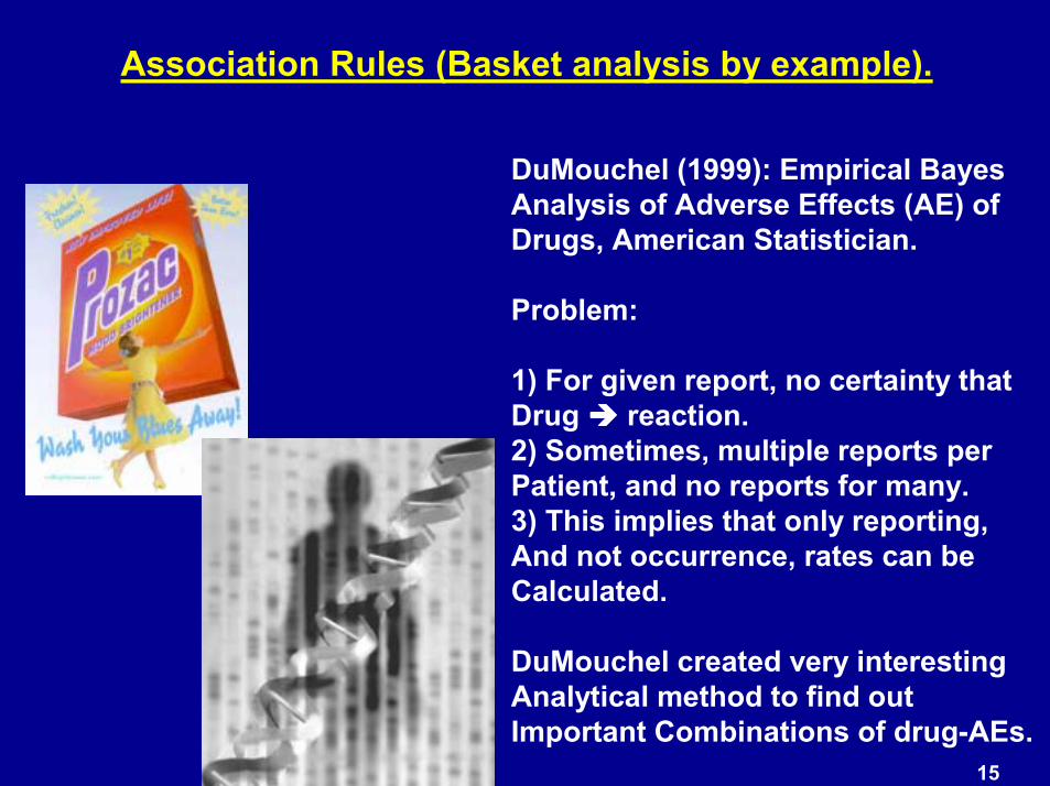
Association Rules (Basket analysis by example).
DuMouchel (1999): Empirical BayesAnalysis of Adverse Effects (AE) of Drugs, American Statistician.
Problem:
1) For given report, no certainty that Drug ���� reaction. 2) Sometimes, multiple reports per Patient, and no reports for many.3) This implies that only reporting, And not occurrence, rates can beCalculated.
DuMouchel created very interestingAnalytical method to find out Important Combinations of drug-AEs.
5/20/0416
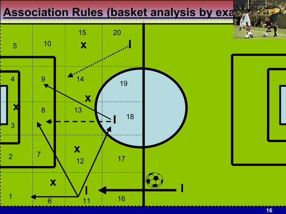
Association Rules (basket analysis by example).
x
x
x
x
x
I I
I
I
1
2
3
4
5
6
7
8
9
10
11
12
13
14
15
16
17
18
19
20
5/20/0417
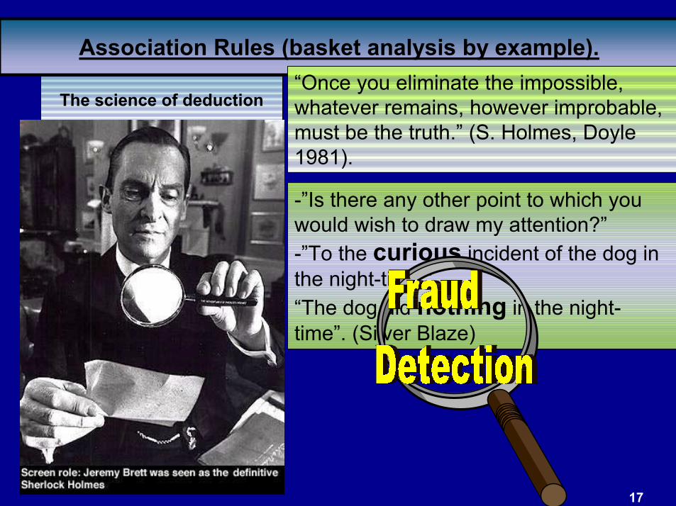
Association Rules (basket analysis by example).
The science of deduction�Once you eliminate the impossible, whatever remains, however improbable, must be the truth.� (S. Holmes, Doyle 1981).
-�Is there any other point to which you would wish to draw my attention?�-�To the curious incident of the dog in the night-time.��The dog did nothing in the night-time�. (Silver Blaze)
5/20/0418
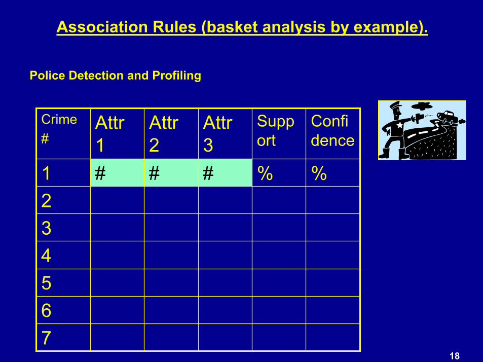
Association Rules (basket analysis by example).
Police Detection and Profiling
765432
%%###1
Confidence
Support
Attr3
Attr2
Attr1
Crime#

5/20/0419
Association Rules (basket analysis by example).
1) Analysts studied voters� survey of 2000 US election.
2) Did Clustering and Tree Modeling: un-interpretable and non-intuitive results.
3) Had 1800 variables plus voter preference.
4) By careful �expert� perusal of rules generated, found �profiles� to identify party preference. For instance, that �female voters, with kids at home �.�.
5) Was also able to generalize by party preference. For instance, �Republicans may share similar backgrounds and a consensus of views within their party more than Democrats or Independents do.�
Analysis of Voter�s preferences (MacDougall, 2003).

5/20/0420
Association Rules (basket analysis by example).
Recommender systems.
1) Amazon.com: �Readers who purchased this item, also purchased ��
2) Point of Sale Retail coupons: �Bought product of brand A, receive coupon for same product from brand B�.
3) E-mail (spam) and snail solicitations due to web browsing, charity donation, credit card purchase �.
4) Web Search Engines (actually use �Link Analysis�). Some use Neural Networks in addition for clustering.

5/20/0421
Slight Detour: Link Analysis.
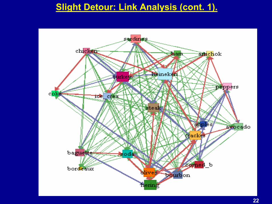
Link Analysis (LA) reveals and visually represents complex patterns of correlations between individual values of categorical and Boolean attributes.
Results of analysis are displayed as graph of linked objects supporting various object manipulation and drill-down operations.
Visual output of LA facilitates better understanding of hidden structure of investigated data, and helps to quickly isolate interesting patterns for further investigation.
5/20/0422
Slight Detour: Link Analysis (cont. 1).

5/20/0423
Slight Detour: Link Analysis (cont. 2).
5/20/0424
Slight Detour: Link Analysis (cont. 3).
Database Marketing. Reveal typical characteristics of the best customers; identify frequent patterns in purchase behavior.
Fraud Detection. Uncover and flag as suspicious those provider-patient or patient-procedure or customer-business pairs that demonstrate unusually high correlations.
Communications Analysis. Visualize main communication patterns and potential network bottlenecks.
Criminal Investigations. Display overall organizational structure, identify articulation points, and trace money laundering and illegal goods transfer patterns.
Text Analysis. Ability to visually display clusters of terms extracted from textual notes to further investigate correlations.
5/20/0425
Association Rules. Lingo.
Association or Market Basket analysis was �the� tool that brought in the term �Knowledge Discovery�.
Another piece of lingo is that data contains precious �Nuggets� of information that can be �mined�, and that brought in the label �Data Mining�.
Artificial Intelligence and Machine Learning were closer to robotic investigation and neural networks. Statisticians� interest in the latter brought the fields closer.
5/20/0426
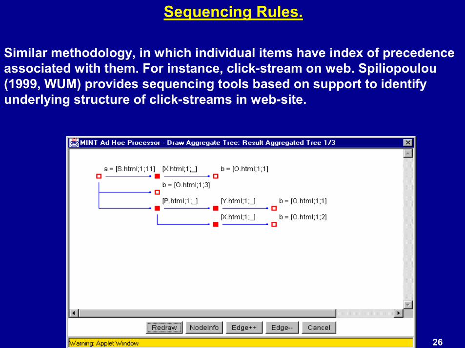
Sequencing Rules.
Similar methodology, in which individual items have index of precedence associated with them. For instance, click-stream on web. Spiliopoulou (1999, WUM) provides sequencing tools based on support to identify underlying structure of click-streams in web-site.

5/20/0427
Analogy.
Since every item in every rule denotes implicitly presence or absence of the item in every rule, each rule can also be considered to be a representation of all available items as dummy variables, where a �0� denotes absence of a specific item, and �1� its presence.
Thus, if there are 5 UPCs in rule studied by retailer, rules could be considered to be as presented in following table.
76
���5�
������
�
3 001112110011
UPC 5UPC 4UPC 3UPC 2UPC 1Rule
4
5/20/0428
Analogy (cont.1).
Therefore, if every rule (adding its negative rule as well as additional variables) can be linked to characteristic important to business, such as total expenditure (and remembering that the rules don�t incorporate quantities), a regression like environment to explain total expenditure is possible.
From it, insights into elasticity estimation are possible, for instance.
5/20/0429
5/20/0430
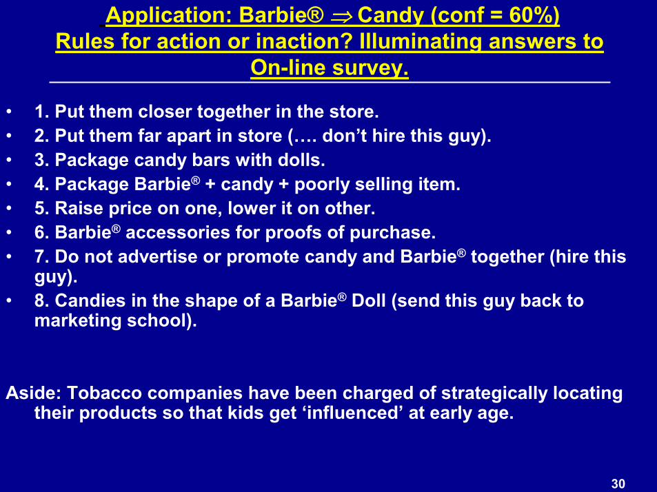
� 1. Put them closer together in the store.� 2. Put them far apart in store (�. don�t hire this guy). � 3. Package candy bars with dolls.� 4. Package Barbie® + candy + poorly selling item.� 5. Raise price on one, lower it on other.� 6. Barbie® accessories for proofs of purchase.� 7. Do not advertise or promote candy and Barbie® together (hire this
guy).� 8. Candies in the shape of a Barbie® Doll (send this guy back to
marketing school).
Aside: Tobacco companies have been charged of strategically locating their products so that kids get �influenced� at early age.
Application: Barbie® ���� Candy (conf = 60%)Rules for action or inaction? Illuminating answers to
On-line survey.

5/20/0431
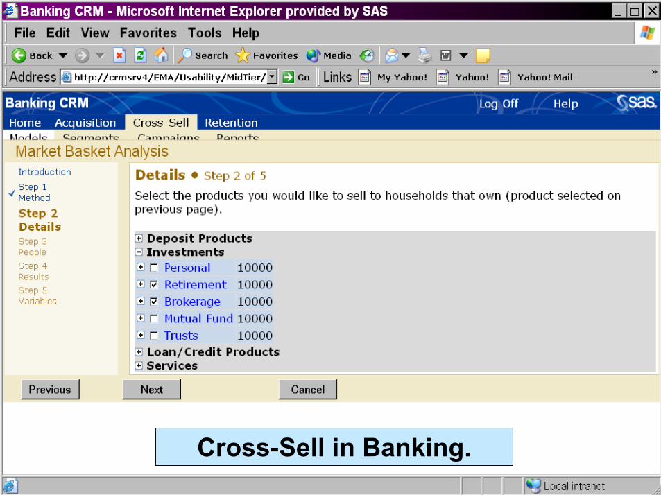
Cross-Sell in Banking.
5/20/0432
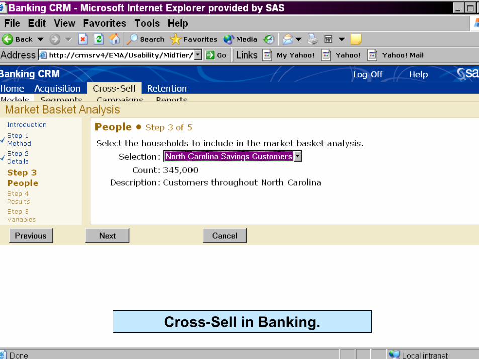
Cross-Sell in Banking.
5/20/0433
Cross-Sell in Banking.

5/20/0434
Cross-Sell in Banking.

5/20/0435
General Observations.
1) Banking case seems to provide well defined and intelligible information of the form:
account_1 and account_2,,, etc or activity_1 and activity_2, etc, possibly indexed by time.
As such, rules found provide guide to action to �offer� product or service (cross-sell).
Note that political survey and police criminal profiles can also be used to produce �offers� to the found profiles.
2) Sherlock Holmes example shows that lack of attribute creates interesting profile for solution.

5/20/0436
General Observations (cont. 1).
3) In retailing case of items purchased together, �guidance� is not so clear cut due to extensive number of rules. However, more extensive analysis and possible solution is presented below.
4) Soccer event exemplifies sequencing of events towards reaching goal. Basketball-applied software has been developed years ago. Web-mining shares the same principles, without passion usually associated with sports.
5) Unit of analysis is problem dependent. In retailing, the unit is each transaction, independent of the customer�s identity. Thus, small group of habitual shoppers may skew results. In clinical data analysis, the unit is patient, who contributes single observation.

5/20/0437
5/20/0438
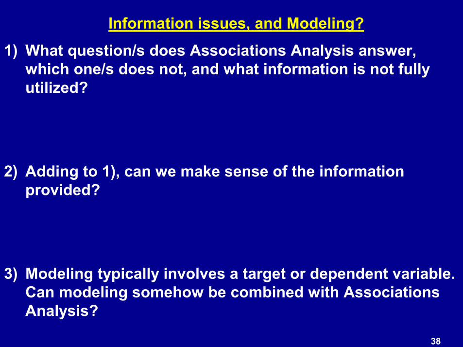
Information issues, and Modeling?
1) What question/s does Associations Analysis answer, which one/s does not, and what information is not fully utilized?
2) Adding to 1), can we make sense of the information provided?
3) Modeling typically involves a target or dependent variable. Can modeling somehow be combined with Associations Analysis?

5/20/0439
What questions are answered?
76
���5�
������
�
3 001112110011
UPC 5
UPC 4
UPC 3
UPC 2
UPC 1
Rule
4
1) Generated rules are different combinations of K dummy variables.Rules over pre-specified support 5%) and only those with �present� effects (�1�) are typically reported.
2) This implies that �seemingly� variable selection effect of association analysis is at best illusory. That is, if �correct� set of variables is not analyzed, there is no rule to indicate that the findings �fit� to maximize profits, to diagnose a disease correctly, etc.

5/20/0440
Biggest issue: is this informative? Example: SAS Enterprise Miner
Association Node (clipped) set of rules
If number of rules �discovered� is, say, 500, how can we conceptualize hidden information, if any?or do we merely consider this counting exercise (similar to accounting) with massive reporting printouts?

5/20/0441
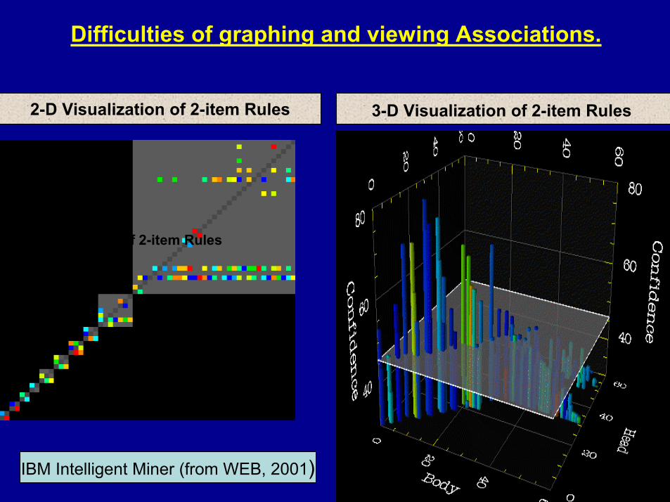
Difficulties of graphing and viewing Associations.
Enterprise MinerV3.01
5/20/0442
Difficulties of graphing and viewing Associations.
3-D Visualization of 2-item Rules
3-D Visualization of 2-item Rules
2-D Visualization of 2-item Rules
IBM Intelligent Miner (from WEB, 2001)
5/20/0443
Additional Issues.
Present methodology does not allow for different amounts of items. I.e., there is no way to relate rule �3 pairs of socks ���� 3 pairs of shoes� with the rule �1 pair of socks ���� 1 pair of shoes�, nor with any �1 watermelon ���� 1 pair of socks�. Quantities alter the meaning of items.
There is no �interestingness� measure. Interestingness is provided by human brains, if there are any, of course (see Holmes� SilverBlaze above).
Similar to �interestingness�, �propensity to purchase�, �probability of contracting a disease�, etc, are interpretations that must beprovided by a business case analysis, a scientific model, or sheer common sense, if any.
5/20/0444
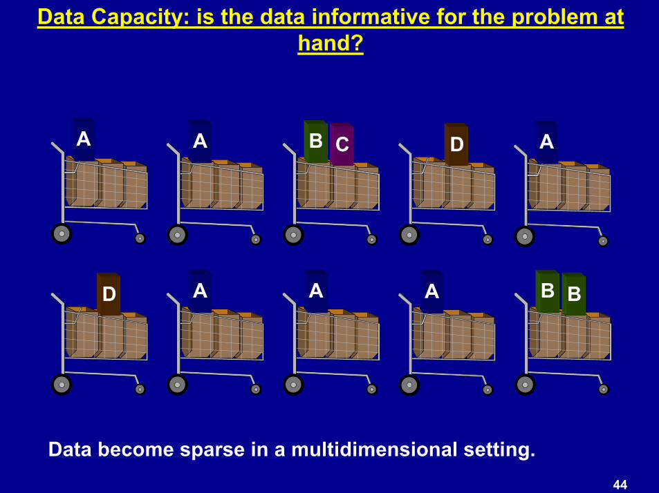
Data Capacity: is the data informative for the problem at hand?
A A B C D A
D A A B BA
Data become sparse in a multidimensional setting.
5/20/0445
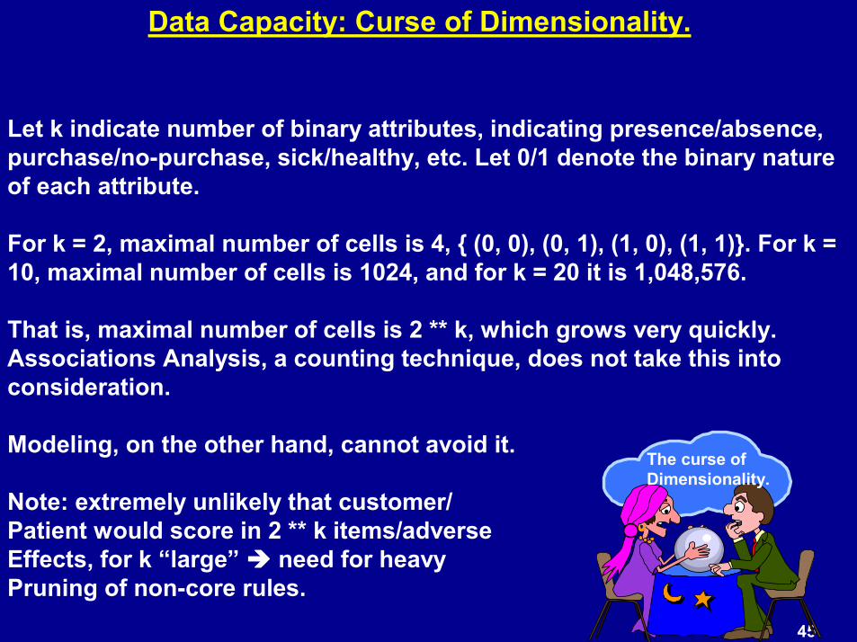
Data Capacity: Curse of Dimensionality.
Let k indicate number of binary attributes, indicating presence/absence, purchase/no-purchase, sick/healthy, etc. Let 0/1 denote the binary nature of each attribute.
For k = 2, maximal number of cells is 4, { (0, 0), (0, 1), (1, 0), (1, 1)}. For k = 10, maximal number of cells is 1024, and for k = 20 it is 1,048,576.
That is, maximal number of cells is 2 ** k, which grows very quickly. Associations Analysis, a counting technique, does not take this into consideration.
Modeling, on the other hand, cannot avoid it.
Note: extremely unlikely that customer/Patient would score in 2 ** k items/adverseEffects, for k �large� ���� need for heavyPruning of non-core rules.
The curse of Dimensionality.

5/20/0446

5/20/0447
Odds and Odds Ratios.Example: Location Preference of Soldiers training in WWII (North/South)
(Rudas, 1998)
3,027959
9583,092
Personal Preference. N SOrigin
NS
4,051(50.4%) 3985(49.6%)
Odds (N vs. S) = 4,051/3,985 = 1.02
Odds (N vs. S / N origin) = 3.23Odds (N vs. S/ S origin) = 0.32
�Suspect association between origin and preference.
Similarly, there is association between present location and preference. Which one is stronger, and how are they related?
Strength: odd ratios; Relation: conditional Odd ratios.
Total = 8,036

5/20/0448
Let π = Probability of success = Pr (Y = 1 / X = 1); and (1 � π) = Pr (Y = 1 / X = 0).
Odds (Y = 1) = Ώ = π / (1 � π) >= 0.
When Ώ > 1 ���� success more likely than failure. Odds equally defined for Y = 0 ����
(1 - π2)π2
(1 - π1)(π12)
π1
(π11)Y
1
0
x1 0
2-way Contingency Table � Conditional Probabilities.
Odds and Odds Ratios (cont. 2).
5/20/0449
Odds and Odds Ratios (cont. 3).
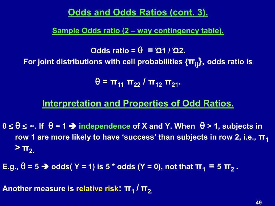
Sample Odds ratio (2 � way contingency table).
Odds ratio = θθθθ = Ώ1 / Ώ2.For joint distributions with cell probabilities {πij}, odds ratio is
θθθθ = π11 π22 / π12 π21.
Interpretation and Properties of Odd Ratios.
0 ≤≤≤≤ θθθθ ≤≤≤≤ ∞. If θθθθ = 1 ���� independence of X and Y. When θθθθ > 1, subjects in row 1 are more likely to have �success� than subjects in row 2, i.e., π1 >π2.
E.g., θθθθ = 5 ���� odds( Y = 1) is 5 * odds (Y = 0), not that π1 = 5 π2 .
Another measure is relative risk: π1 /π2.

5/20/0450
Odds and Odds Ratios (cont. 4).
Estimated odd ratio: θθθθ(hat) = n11 n22 / n12 n21., which equals 0 or ∞ if any element is 0, and undefined if any two entries in numerator and denominator are 0.
The distribution of θθθθ(hat) is highly skewed because, unless n is very large, the lower bound is 0 and the upper one is ∞ with non-negligible probability.
���� log-transform that converges to normality more quickly.
Estimated SE for log( θθθθ(hat)) = σ(hat) (θθθθ(hat)) =
By asymptotic normality, the CI is:
Log θθθθ(hat) + | z αααα/2 σ(hat) (θθθθ(hat))|
2 2
( 1/ )iji j
sqrt n��

5/20/0451
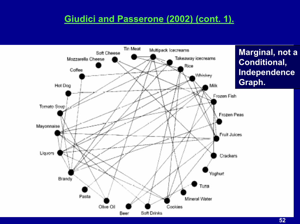
Giudici and Passerone (2002).
Giudici�s and Passerone�s (2002) approach focuses on pairs of grocery items. Given K items, form all K (K � 1) / 2 contingency tables, and conclude that pair of items is associated whenever odds ratio,corresponding to marginal independence, lies outside confidence interval of odds = 1.
They also provide graphical description of relations, borrowed from link analysis, which shows 36 dependency relations, given by edges of the graph. They focus analysis then on absolute odd ratios significantly larger than 5, which leads them to 5 �clusters�, completely disconnected from each other.
Promotional variables are then added to each cluster, and check whether promotions affect sales. They analyze one cluster in the paper.
5/20/0452
Giudici and Passerone (2002) (cont. 1).
Marginal, not aConditional,IndependenceGraph.
5/20/0453
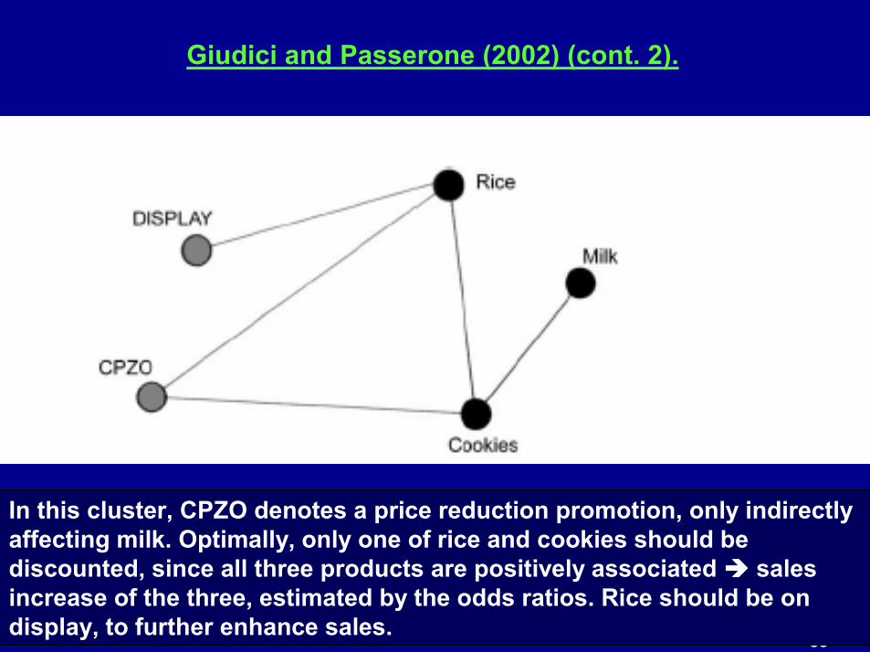
Giudici and Passerone (2002) (cont. 2).
In this cluster, CPZO denotes a price reduction promotion, only indirectly affecting milk. Optimally, only one of rice and cookies should be discounted, since all three products are positively associated ���� sales increase of the three, estimated by the odds ratios. Rice should be on display, to further enhance sales.

5/20/0454
Giudici and Passerone (2002) (application).
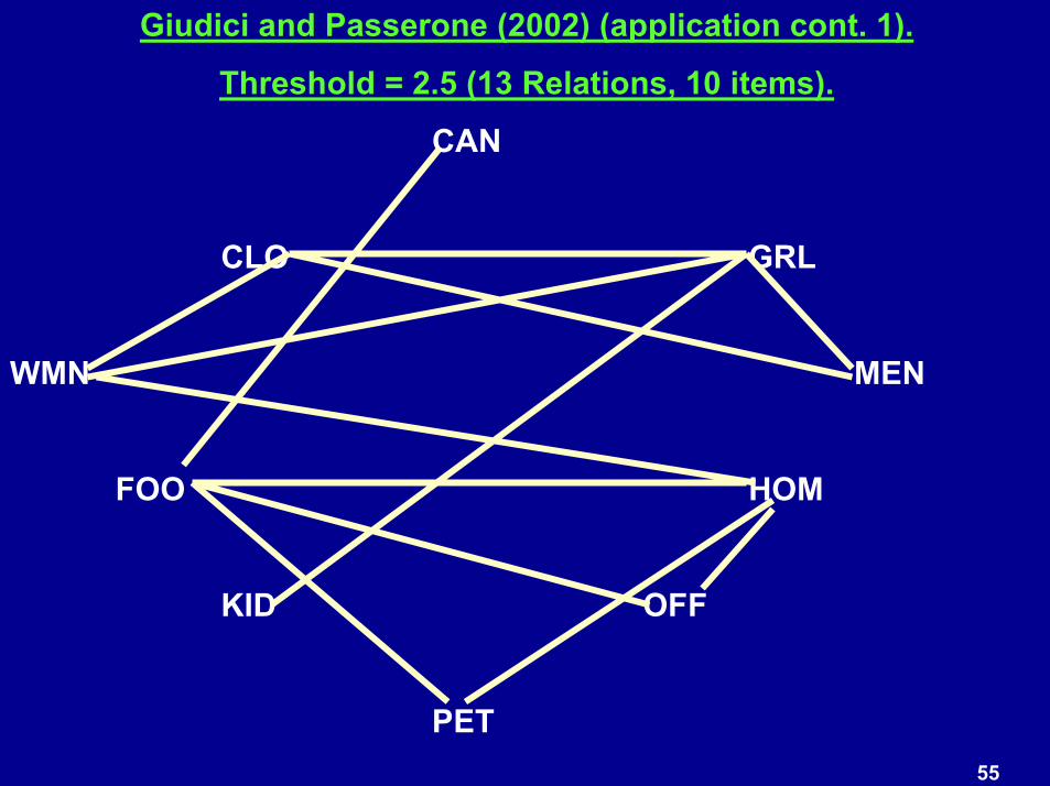
Retailer has some transaction data for 15 categories of products: CAN(dy) CLO(thing) CRA(fts) GRL WMN MEN FOO(d) FUN HLT(health) HOM(e) HRD(hardware) JWL(jewelry) KID OFF(ice) PET.
Threshold for Odds_ratio = 3 ���� 2 disjoint clusters (different colors).
FOO WMN
CAN CLO
GRL MEN
OFF
HOME PET
5/20/0455
Giudici and Passerone (2002) (application cont. 1).
Threshold = 2.5 (13 Relations, 10 items).
CAN
CLO GRL
WMN MEN
FOO HOM
KID OFF
PET

5/20/0456
Giudici and Passerone (2002) (application cont. 2). Threshold = 2 (19 relations, 12 items).
CAN CRA
CLOGRL WMN
MEN FOO
HLT HOM
KID OFF
PET

5/20/0457
-0. 80
0. 11
1. 02
1. 93
2. 84
DIM 1
-0. 85 -0. 33 0. 18 0. 70 1. 21

5/20/0458

5/20/0459
Danger: Simpson�s Paradox (1951).
In general, we expect that aggregates should evince same relationshipsas the categories, levels or individuals over which aggregate was formed.
Simpson�s paradox: Direction of association is reversed when third variable is introduced. It happens rarely in actual practice but may happen more often the more you search.
Bickel et al (1975) example: apparent gender bias in acceptances to graduate school at Berkeley in 1973. As a whole, males were accepted proportionately more than females. However, at the individual department level, reverse was happening.
Females had overall lower rate of admission because they applieddisproportionately more often to departments with lowest rates of acceptance.
5/20/0460
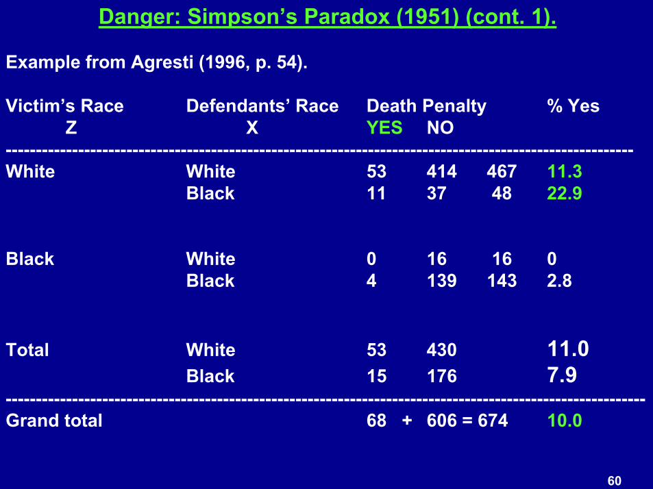
Danger: Simpson�s Paradox (1951) (cont. 1).
Example from Agresti (1996, p. 54).
Victim�s Race Defendants� Race Death Penalty % YesZ X YES NO
--------------------------------------------------------------------------------------------------------White White 53 414 467 11.3
Black 11 37 48 22.9
Black White 0 16 16 0Black 4 139 143 2.8
Total White 53 430 11.0Black 15 176 7.9
----------------------------------------------------------------------------------------------------------Grand total 68 + 606 = 674 10.0
5/20/0461
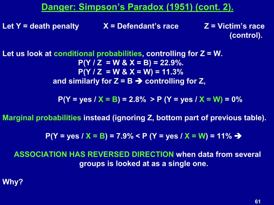
Danger: Simpson�s Paradox (1951) (cont. 2).
Let Y = death penalty X = Defendant�s race Z = Victim�s race (control).
Let us look at conditional probabilities, controlling for Z = W.P(Y / Z = W & X = B) = 22.9%.P(Y / Z = W & X = W) = 11.3%
and similarly for Z = B ���� controlling for Z,
P(Y = yes / X = B) = 2.8% > P (Y = yes / X = W) = 0%
Marginal probabilities instead (ignoring Z, bottom part of previous table).
P(Y = yes / X = B) = 7.9% < P (Y = yes / X = W) = 11% ����
ASSOCIATION HAS REVERSED DIRECTION when data from several groups is looked at as a single one.
Why?
5/20/0462
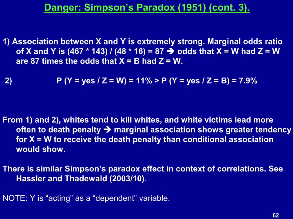
Danger: Simpson�s Paradox (1951) (cont. 3).
1) Association between X and Y is extremely strong. Marginal odds ratio of X and Y is (467 * 143) / (48 * 16) = 87 ���� odds that X = W had Z = W are 87 times the odds that X = B had Z = W.
2) P (Y = yes / Z = W) = 11% > P (Y = yes / Z = B) = 7.9%
From 1) and 2), whites tend to kill whites, and white victims lead more often to death penalty ���� marginal association shows greater tendency for X = W to receive the death penalty than conditional association would show.
There is similar Simpson�s paradox effect in context of correlations. See Hassler and Thadewald (2003/10).
NOTE: Y is �acting� as a �dependent� variable.
5/20/0463
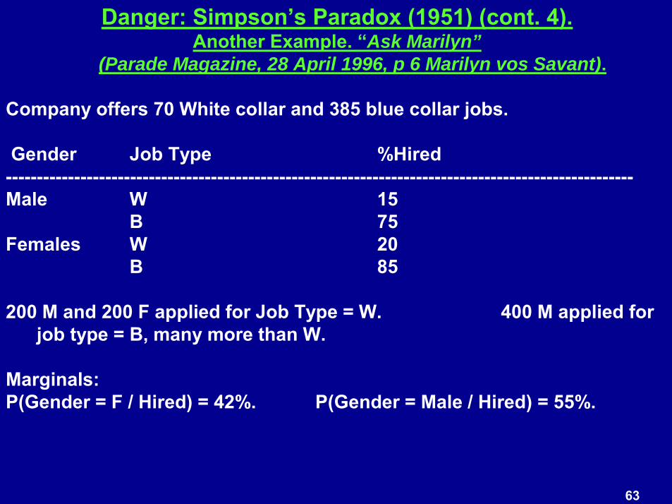
Danger: Simpson�s Paradox (1951) (cont. 4).Another Example. �Ask Marilyn”
(Parade Magazine, 28 April 1996, p 6 Marilyn vos Savant).
Company offers 70 White collar and 385 blue collar jobs.
Gender Job Type %Hired-----------------------------------------------------------------------------------------------------Male W 15
B 75Females W 20
B 85
200 M and 200 F applied for Job Type = W. 400 M applied for job type = B, many more than W.
Marginals: P(Gender = F / Hired) = 42%. P(Gender = Male / Hired) = 55%.

5/20/0464
Danger: Simpson�s Paradox (1951) (cont. 5).Another Example (derived from EdStat-L, 2/25/04).
Fast food manager restaurant argues that 75% or more of visits are drive-through. Analyst collects 50 days of data to test hypothesis and his point estimate is proportion of drive-through visits. However, his estimate may be Simpsonially affected:
Drive-through(Y, N, %)
Tue 30 10 .75Wed 30 10 .75Thu 30 10 .75Fri 30 90 .25Sat 30 90 .25Sun 30 90 .25
___________________________
======= Total 180 300 0.375
5/20/0465
To Simpson or not to Simpson.
Be extremely CAREFUL when generalizing over aggregated data. Associations analysis provides huge amounts of support, confidence and lift measures, which are marginal and conditional probabilities.
Since practice is lift > 1 ���� look at �interesting� confidence, ensure that Simpson is not lurking by looking at rules with previous conditioners omitted.
Thus, if A & B ���� C is �interesting�, look also at A ���� C, B ���� C., etc.

5/20/0466
5/20/0467
Other Methods.
1) Association Tree Tool (Liu et al. 1998): creates a tree structure based on descending Confidence and prunes upwards based on misclassification rate.
2) Association Chi-Square (Auslender, 2000a and 2000b): Items deemed �dependent� per Chi-Square test become �composites� and search continues until no more composites are possible.
3) Terse Representation of AA (Auslender, 2002): Obtains regression type representation of items, thus simplifying conceptualization.
4) Naïve-Bayes: One item becomes dependent variable. NB �learns� classification rules transactions and classifies future transactions where true nature of dependent variable is unknown. Main assumption is that explanatory items are independent.
5/20/0468
Other Methods (cont. 1).
5) Bayesian Networks: Directed A-Cyclical Graphical Models. Items are variables that are linked by probability statements. Masuda et al (1999) performed a study linking up AA and BNs.
6) Wu et al (2003) propose log-linear model to summarize results from AA.

5/20/0469

5/20/0470
Conclusions and future development.1) Despite �discovery� claims by data miners, ridiculously extended reports of groups of items do not lend themselves easily to conceptual knowledge. Human brains are irreplaceable in this and other situations as well. Columbus was a discoverer, human software is not (see Boorstin, 1985, and very forcefully, Goodman, 2002).

5/20/0471
Conclusions and future development (cont. 1).
2) There are many instances of items with very small supportthat are bypassed by traditional tools. It could well be that itis their rarity that makes these items valuable. Therefore, weighted support (and confidence), or completely different index might be necessary to identify these nuggets of information (Liu et al, 1999).
3) Alternative to searching for �interesting� items is to eliminate �non-interesting� ones. E.g., husband ���� married, orange ���� fruit. Sahar (1999) provides recursive algorithm for this. Of course, if we find �husband ���� unmarried�, either data base information needs cleaning, or else civil laws of nation have changed, or �
5/20/0472
Conclusions and future development (cont. 2).4) Padmanabhan and Tuzhilin (1998) created an algorithm where �interestingness� is provided as contradiction toestablished beliefs. The beliefs are elicited from experts or derived from perusing the data.
5) Associations Analysis can also be understood within framework of Bayesian Networks. With on-going developments of algorithms to identify structure from data, it is possible to venture much further in simplifying the information provided. Still, present applied work has not revealed full potential of the method.
6) Giudici�s and Passerone�s approach is easy to investigate. Choice of magical �5� is easily modifiable.

5/20/0473
5/20/0474
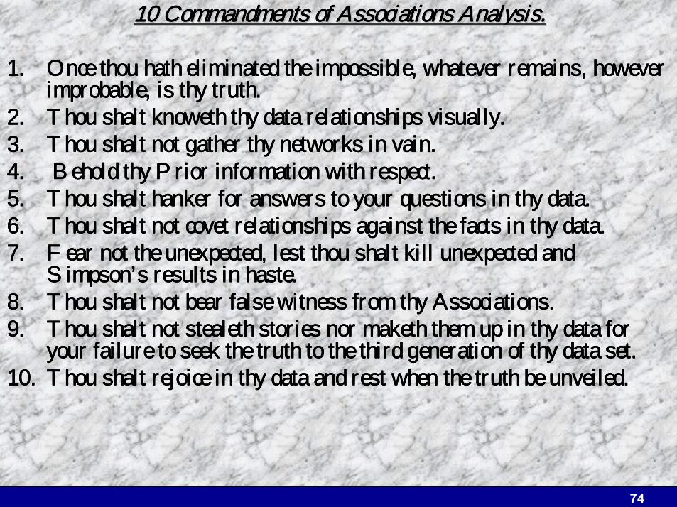
10 Commandments of Associations Analysis.10 Commandments of Associations Analysis.10 Commandments of Associations Analysis.10 Commandments of Associations Analysis.10 Commandments of Associations Analysis.10 Commandments of Associations Analysis.10 Commandments of Associations Analysis.10 Commandments of Associations Analysis.
1.1.1.1. Once thou hath eliminated the impossible, whatever remains, howeOnce thou hath eliminated the impossible, whatever remains, howeOnce thou hath eliminated the impossible, whatever remains, howeOnce thou hath eliminated the impossible, whatever remains, however ver ver ver improbable, is thy truth. improbable, is thy truth. improbable, is thy truth. improbable, is thy truth.
2.2.2.2. Thou shalt knoweth thy data relationships visually.Thou shalt knoweth thy data relationships visually.Thou shalt knoweth thy data relationships visually.Thou shalt knoweth thy data relationships visually.3.3.3.3. Thou shalt not gather thy networks in vain. Thou shalt not gather thy networks in vain. Thou shalt not gather thy networks in vain. Thou shalt not gather thy networks in vain. 4.4.4.4. Behold thy Prior information with respect. Behold thy Prior information with respect. Behold thy Prior information with respect. Behold thy Prior information with respect. 5.5.5.5. Thou shalt hanker for answers to your questions in thy data.Thou shalt hanker for answers to your questions in thy data.Thou shalt hanker for answers to your questions in thy data.Thou shalt hanker for answers to your questions in thy data.6.6.6.6. Thou shalt not covet relationships against the facts in thy dataThou shalt not covet relationships against the facts in thy dataThou shalt not covet relationships against the facts in thy dataThou shalt not covet relationships against the facts in thy data....7.7.7.7. Fear not the unexpected, lest thou shalt kill unexpected and Fear not the unexpected, lest thou shalt kill unexpected and Fear not the unexpected, lest thou shalt kill unexpected and Fear not the unexpected, lest thou shalt kill unexpected and
Simpson’s results in haste.Simpson’s results in haste.Simpson’s results in haste.Simpson’s results in haste.8.8.8.8. Thou shalt not bear false witness from thy Associations. Thou shalt not bear false witness from thy Associations. Thou shalt not bear false witness from thy Associations. Thou shalt not bear false witness from thy Associations. 9.9.9.9. Thou shalt not Thou shalt not Thou shalt not Thou shalt not stealeth stealeth stealeth stealeth stories nor maketh them up in thy data for stories nor maketh them up in thy data for stories nor maketh them up in thy data for stories nor maketh them up in thy data for
your failure to seek the truth to the third generation of thy dayour failure to seek the truth to the third generation of thy dayour failure to seek the truth to the third generation of thy dayour failure to seek the truth to the third generation of thy data set. ta set. ta set. ta set. 10.10.10.10. Thou shalt rejoice in thy data and rest when the truth be unveilThou shalt rejoice in thy data and rest when the truth be unveilThou shalt rejoice in thy data and rest when the truth be unveilThou shalt rejoice in thy data and rest when the truth be unveiled.ed.ed.ed.

5/20/0475
5/20/0476
Agrawal R., Imielinski T., and Swami A. (1993), Mining association rules between sets of items in very large databases, Proceedings of the ACM SIGMOD Conference on Management of data, pages 207-216, Washington D. C.
Agresti A. (1996): An Introduction to Categorical Data Analysis, Wiley.
Agresti A. (1998): Applied Categorical Data Analysis, Wiley.
Auslender, Leonardo (2000a): On Analytical Tools for Market Basket Analysis, Proceedings of the Diamond SAS Users Group Conference.
Auslender L. (2000b), “On visualizing Direct and Partial Correlations – ELI plots”, Proceedings of the Diamond-SUG Meeting, San Francisco,
Auslender L. (2002): On terse representations of Associations Analysis, ART Forum.
Bickel P., Hammel E., O�Connell J. (1975): Sex bias in graduate admissions: Data from Berkeley, Science, 187, 398-404.
5/20/0477
Boorstin D., The Discoverers, Vintage Books, 1985.
Doyle A. C. (1981): The Celebrated Cases of Sherlock Holmes, Octopus Books Limited.
DuMouchel W. (1999): Bayesian Data Mining in Large Frequency Tables, with an application to the FDA Spontaneous Reporting System, The American Statistician.
Giudici P., Passerone G. (2002): Data Mining of Association Structures to model consumer behavior, Computational Statistics and Data Analysis, 38, 4, 533-541.
Goodman A. Challenges, Checklists and Scorecards for Data Miners, Statisticians and Clients who fund them, presented at the SAS 2002 Data Mining Conference, 2002.
Hassler U. and Thadewald T. (2003, October): Nonsensical and Biased Correlation due to pooling heterogeneous samples, The Statistician, 52, Part 3, pp. 367-379.
5/20/0478
Liu Bing, Hsu Wynne and Ma Yiming (1998), Integrating Classification and Association Rule Mining, Proceedings of The Fourth International Conference on Knowledge Discovery & Data Mining, New York.
Liu B., Hsu W., Ma Y. (1999): Mining Association Rules with multiple Minimum Supports, Proceedings of the 1999 Knowledge Discovery & Data Mining.
MacDougall M. (2003): Shopping for Voters: Using Association Rules to discover relationships in Election Survey Data, Proceedings of the SAS Users Group International.
Masuda G., Yano R., Sakamoto N., Ushijima K. (1999): Discovering and Visualizing Attribute Associations Using Bayesian networks and their use in KDD, Proceedings of the 3rd European Conference on Principles of DMKD (PKDD-99), LNAI, vol. 1704, pp. 61-70, Springer-Verlag.
Megiddo Nimrod and Srikant Ramakrishnan (1998), Discovering Predictive Association Rules, Proceedings of The Fourth International Conference on Knowledge Discovery & Data Mining, New York.

5/20/0479
Padmanabhan B., Tuzhilin A. (1998): A belief-driven method for discovering unexpected patterns, Proceedings of the 1998 Conference on Knowledge Discovery & Data Mining.
Rudas T. (1998): Odds Ratios in the Analysis of Contingency Tables, Sage.
Sahar S. (1999): Interestingness via what is not interesting, Proceedings of the 1999 conference on Knowledge Discovery & Data Mining.
Simpson, E. H. (1951), The Interpretation of Interaction in ContingencyTables, Journal of the Royal Statistical Society, Ser. B, 13, 238-241.
Spiliopoulou, M.: (1999/03): Laborious way from data mining to web mining, Computer Systems, Science & Engineering.
Tan P., Kumar V., Srivastava J. (2002): Selecting the Right InterestingnessMeasure for Associations Patterns, Proceedings of the 8th ACM SIGKDD International Conference on KDD, pp. 32-41, 2002.
5/20/0480
Wu X., Barbara D., Ye Y. (2003): Screening and Interpreting Multi-Item Associations Based on Log-Linear Modeling, Proceedings of the 2003 KDD Conference on DMKD.

5/20/0481