Embed Size (px)
Citation preview
On aftermarkets, network e¤ects and dynamic competitionfor locked in consumers
Didier LausselGREQAM and Université de la Mediterranée
E-mail:
and
Joana Resende1
CORE, Université catholique de Louvain and CETE, Universidade do PortoE-mail: [email protected]
Version: April 28, 2009
In this paper, we propose a theoretical model of dynamic competition in primary markets and
aftermarkets, explicitly accounting for the network e¤ects resulting from the interplay between the value
of complementary goods and services (sold in aftermarkets) and the size of the network in the primary
market. Relying on the equilibrium notion of Linear Markov Perfect Equilibrium, we investigate market
outcomes at equilibrium. We conclude that equilibrium prices in the primary market tend to be lower
when durable goods traded in primary markets are weakly di¤erentiated, competition in aftermarkets is
relatively soft, the intrinsic utility of complementary goods and services is high and network e¤ects are
considerably intense.
Key Words: Aftermarkets, network e¤ects, di¤erential games, linear Markov perfect equi-
librium
1. INTRODUCTION
In several durable-goods markets (primary markets) the value of the durable-good / equip-
ment is essentially derived from using it complementarily with goods and services sold in other
markets (aftermarkets): cars and maintenance/repairing services, printers and ink cartridges,
co¤ee machines and co¤ee capsules, hardware and software,... Moreover, in several cases, the
interplay between primary markets and aftermarkets entails network e¤ects: often, the value of
the complementary goods and services (CGS) is positively related to the number of consumers
who are endowed with a similar equipment in the primary market. For example, the larger the
number of consumers buying a speci�c printer, the easier it is to �nd a seller of the corresponding
ink cartridges. Similarly, the availability of adequate co¤ee capsules increases with the number
1The authors thank Paul Belle�amme, António Brandão, So�a Castro, Jean Gabszewicz, Filomena Garcia,Ngo Van Long, Paula Sarmento for their helpful comments. Joana Resende acknowledges �nancial support fromCETE, Universidade do Porto and FCT.
1
of consumers owning a compatible co¤ee machine. Also, the availability and the quality of PC
(vsus Mac) assistance/repairing services is positively related with the total number of PC users
(vsus Mac users)2 .
A number of recent antitrust cases, like Eastman Kodak Co. v. Image Technical Servs
(copiers and maintenance/reparation services); Pelikan v. Hewlett-Packard (printers and ink
cartridges), Canada (Director of Investigation and Research) v. Chrysler Canada, Ltd. (auto-
mobile industry), Red Lion Medical Safety, Inc. v. Ohmeda, Inc (medical equipment).... have
dealt with antitrust issues arising when equipment producers are also involved in the provision
of CGS. Several aftermarket theories have investigated the interplay between primary markets
and aftermarkets. However, hitherto, there are no consensual results regarding the rationale for
antitrust intervention in aftermarkets. Some of these theories tend to be favorable to antitrust
intervention (e.g. Borenstein et al, (2000)), claiming that welfare losses entailed by the lack
of competition in aftermarkets are not ruled out by competition in primary markets. In con-
trast, some theories3 are less prone to support antitrust intervention in aftermarkets, arguing
that consumers� injury caused by the lack of competition in aftermarkets tends to be rather
small, especially when primary markets are competitive (e.g. Shapiro (1995)). Other theories
go even further, pointing that the lack of competition in aftermarkets may be welfare-improving
in certain situations (even from consumers�point of view). For example, that can be the case
when there are increasing returns in the aftermarkets (Cabral (2008)), when there is uncertainty
about equipment�quality (Schwartz and Werden (1996)), or when there are problems due to time
inconsistency related with durable-goods (Morita and Waldman (2004), Carlton and Waldman
(2001)).
In this paper, we develop a theoretical model of dynamic competition in primary markets
and aftermarkets. In line with the previous literature, our model takes into account the following
features of aftermarkets: (i) goods/ services traded in aftermarkets aim to complement a durable
good, whose value considerably depends on CGS consumption; (ii) equipment choices precede
consumers�purchases of CGS; and (iii) consumers are signi�cantly "locked in" to their equipment
and therefore, the switch from one equipment�brand to another is highly unlikely. In addition,
we formally introduce in our model the network e¤ects resulting from the interplay between the
value of CGS and the size of the installed base of equipment owners.
The model used in this paper corresponds to a di¤erential game with a linear-quadratic
structure. To investigate agents� optimal decisions and equilibrium market outcomes in the
context of this dynamic game, we rely on the equilibrium concept of Linear Markov Perfect
Equilibrium (LMPE). This equilibrium concept rests on two assumptions. On the one hand, it is
assumed that all the payo¤ relevant information can be summarized by the state vector (Markov
perfection). On the other hand, the concept of LMPE is restricted to equilibrium strategies that
2As a matter of fact, quite often, there are learning e¤ects in the provision of CGS. In those circumstances,the expertise of CGS suppliers positively depends on the number of consumers endowed with the correspondingequipment.
3For example, Chen and Ross (1993), Shapiro (1995), Schwartz and Werden (1996), Carlton and Waldman(2001), Morita and Waldman (2004), Cabral (2008),...
2
can constitute a¢ ne functions of the state vector. The �rst assumption is quite common in the
literature dealing with problems of dynamic price competition in network industries (see Cabral
(2008), Mitchell and Skrzypacz (2006), Laussel et al (2004), Doganoglu (2003),...). Concerning
the second assumption, our game being linear-quadratic, it is natural to search for the simplest
equilibrium strategies that solve linear-quadratic games, namely, the linear strategies.
We provide a necessary and su¢ cient condition for the existence of a unique LMPE in which
both �rms have non-negative market shares. When such a unique equilibrium exists, instan-
taneous equilibrium prices in the primary market depend on (i) the degree of di¤erentiation
between the available equipment variants; (ii) the pro�tability of the corresponding aftermar-
kets; and (iii) the relative market shares of each equipment variant in the primary market.
As concerns (i), it is not surprising that equipment prices tend to be lower when equipment
variants are more similar. Regarding (ii), we show that equipment prices are negatively correlated
with the pro�tability of aftermarkets, which depends itself on: the degree of competition in
aftermarkets, the intrinsic value of CGS and the intensity of network e¤ects. More precisely,
equipment prices are higher in the case of very competitive aftermarkets or when consumers do
not value that much CGS (either because CGS have a limited intrinsic utility or because they
do not yield a signi�cant network bene�t).
Finally, in relation to (iii), we show that, when we account for the network e¤ects resulting
from the interplay between the value of CGS and the size of the installed base of equipment own-
ers, at each instant of time, the equipment producer with a larger installed base of consumers
sells its equipment at a higher price. The intuition for this result is the following. When account-
ing for network e¤ects, it follows that, ceteris paribus, CGS made available to the "dominant"
equipment4 are more valuable than CGS made available to the other equipment (with a lower
market share) since the network bene�ts yielded by the former are larger than the network ben-
e�ts yielded by the latter. When we concentrate on the unique LMPE in which both �rms have
non-negative market shares, the producer of the dominant equipment exploits its "qualitative
advantage" by setting a higher price than its rival ("fat cat"5 e¤ect).
Along the LMPE trajectories, the dominant equipment becomes less and less likely to capture
new consumers6 and the asymmetry on the market shares of equipment producers tends to vanish
with time (decreasing dominance). Given that we focus on LMPE in which both �rms have non-
negative market shares, it is not surprising that, in the steady state, �rms share the market evenly.
However, it is worth noting that there might be a considerable inertia in the evolution of market
shares towards this symmetric steady state, especially when products are weakly di¤erentiated,
network e¤ects are considerably intense or when the �ows of consumers entering and exiting this
industry are relatively limited.
From a welfare perspective, we show that the exercise of market power in aftermarkets is
always bene�cial to equipment producers and detrimental to consumers who were already en-
4The dominant equipment corresponds to the equipment that is owned by a larger fraction of consumers.5This concept has been introduced by Fudenberg and Tirole (1983).6Furthermore, this e¤ect is reinforced by the fact that the dominant equipment also registers higher exit �ows.
3
dowed with an equipment. Regarding independent CGS suppliers and consumers who were not
initially endowed with an equipment, the e¤ect of restricting competition in aftermarkets is non-
monotonic. Adding up all e¤ects, we conclude that the lack of competition in aftermarkets has
a detrimental e¤ect on "Marshallian social welfare". In our model, the social damage is caused
by the underprovision of CGS due to the lack of competition in aftermarkets7 .
The rest of the paper is organized as follows. Section 2 presents the basic ingredients of the
model. Section 3 and Section 4 respectively investigate agents�decisions in aftermarkets and in
the primary market. Section 5 analyzes market outcomes from a welfare perspective and, �nally,
Section 6 concludes.
2. THE MODEL
Consider a duopolistic primary market, where two �rms (Firm 1 and Firm 2) produce, at zero
marginal cost, in�nitely-lived and horizontally di¤erentiated durable goods (Equipment 1 and
Equipment 2). Horizontal di¤erentiation is modelled à la Hotelling with quadratic transportation
costs8 . The Hotelling line [0; 1] represents the spectrum of all possible equipment variants.
Equipment 1 and Equipment 2 are located at the opposite extremes of this line (Equipment 1
is located at point x1 = 0, while Equipment 2 is located at point x2 = 1). Potential equipment
buyers are uniformly distributed along the Hotelling line, in accordance with their preferences.
We consider that equipment owners face considerable switching costs9 (learning costs, habit
formation,...) and therefore, the switch from one equipment�brand to another never occurs (full
lock in in the primary market). At each instant of time, consumers who are not endowed with an
equipment (new consumers) make a lifetime choice between the two available equipment variants.
To make such choice, consumers compare (i) the intrinsic characteristics of each equipment, (ii)
their respective prices and (iii) the additional value that consumers may extract from their
equipment by using it together with the appropriate CGS throughout their lives.
The expected lifetime utility obtained by a consumer located at x 2 [0; 1] in the Hotellingline who buys equipment i at instant t; is denoted by Vi (x; t) ; i = 1; 2 :
Vi (x; t) =
Z 1
t
h#� � (x� xi)2
ie�(r+�)(v�t)dv +
Z 1
t
E[ui(v)]e�(r+�)(v�t)dv � pi (t) ; (1)
where # > 0 is the instantaneous intrinsic utility10 delivered by the equipment variant corre-
sponding to consumers�most preferred speci�cation; � is the unit transportation cost; r+� is the
"adjusted discount rate", with r standing for the conventional discount rate and � < r2 standing
for the instantaneous probability of exiting the industry; E[ui(v)] corresponds to the expected
utility obtained from CGS consumption at instant v > t; and, �nally, pi (t) denotes the price
7To be more precise, this welfare loss corresponds to the "deadweightloss" triangle arising in aftermarkets.This result is in line with Shapiro (1995) or Borenstein et al (2000).
8See d�Aspremont et al (1979).9On switching costs see, for example, Klemperer (1987) or Farrell and Shapiro (1988).10By intrinsic utiliy, we mean the equipment value that does not depend on CGS consumption.
4
of equipment i at instant t: The constant # is considered to be large enough for all potential
equipment buyers to �nd an equipment for which Vi (x; t) is positive at equilibrium (full mar-
ket coverage). We focus on forward-looking agents, assuming that agents are able to perfectly
anticipate the future bene�ts generated by future consumption of CGS (i.e. E[ui(v)] � ui (v)):
In the aftermarket, two distinct categories of perishable CGS11 are available. Both categories
of CGS are produced at zero marginal cost. We consider that each type of CGS has been
speci�cally designed for a particular equipment variant, being fully incompatible with the other
equipment. Hence, also in the aftermarket, consumers are fully locked in to their equipment:
equipment owners only bene�t from CGS consumption when combining their equipment with the
appropriate category of CGS. Equipment 1 must be combined with CGS1; while Equipment 2
must be combined with CGS2. Accordingly, the aftermarket can be decomposed in two mutually
exclusive market segments: aftermarket of CGS1 (where the owners of equipment 1 buy CGS
throughout their lives) and aftermarket of CGS2 (where the owners of equipment 2 buy CGS
throughout their lives):
In each segment of the aftermarket, the instantaneous utility obtained by a consumer endowed
with equipment i who, at instant t; buys a level gi of CGSi is equal to ui (gi (t) ; Di (t) ; Dj (t)) �ui (t) :
ui (t) = � + �gi (t)�1
2gi (t)
2+ [Di (t) + �Dj (t)]� vi (t) gi (t) ; (2)
where � > 0 is a constant that measures the �xed intrinsic utility of CGSi to the owners of
equipment i; � > 0 is a constant that measures the marginal bene�t of CGS consumption; gi (t)
denotes the level of CGSi consumption by the owners of equipment i; > 0 is a constant
that measures the intensity of network e¤ects; � > 0 is a constant that measures the degree
of compatibility between rival networks; Di (t) and Dj (t) = 1 � Di (t) respectively denote the
fraction of consumers endowed with equipment i and equipment j at instant t; and, �nally, vi (t)
denotes the unit price of CGSi at instant t:
The speci�cation of ui (t) in equation (2) is suitable for aftermarkets exhibiting network
e¤ects associated with the size of equipment� installed base of (locked in) customers in the
primary market. The larger the installed base of consumers endowed with equipment i; the more
valuable CGSi become. We allow for partial compatibility between networks, considering that
the number of consumers endowed with the rival equipment has a positive, albeit smaller, impact
on the value of CGS12 . The degree of compatibility between rival networks is measured by the
parameter �: Note that network e¤ects are incorporated in ui (t) linearly, and consequently, they
do not in�uence the marginal bene�t of CGS consumption.
Concerning the production of CGS, we introduce the possibility of competition in each seg-
ment of the aftermarket. More precisely, we consider that, in each aftermarket segment, the
11Examples of perishable CGS include repairing services, maintenance services, and so on.12For example, in the case of learning e¤ects, partial compatibility refers to the fact that CGS suppliers in
a given segment of the aftermarket may (partially) bene�t from the learning economies generated in anothersegment of the aftermarket, due to knowledge di¤usion/transmission.
5
equipment producer i competes à la Cournot with other N � 1 similar (independent) suppliersof CGS13 , with N � 1. We rule out any commitment device in the aftermarket14 .In this context, we investigate agents�optimal strategies in primary markets and aftermarkets,
considering a dynamic game with the following structure. At each instant of time t; there is
an in�ow of new consumers (arriving in the industry at a rate of �) and an out�ow of old
consumers (exiting the industry at the same rate �): In the primary market, at each instant
of time t; Firm 1 and Firm 2 respectively set p1 (t) and p2 (t) ; accounting for their impact on
�rms� current and future pro�ts. Newborn consumers observe equipment prices and make a
lifetime choice of equipment, taking into consideration equipment prices, their tastes and their
rational expectations on the discounted utilities obtained from CGS consumption throughout
their lifetime. Finally, in each segment of the aftermarket, at each instant of time t; each
equipment producer competes à la Cournot with other independent N �1 suppliers, establishingthe unit-price of CGSi, vi (t) : Conditional on the instantaneous price of CGSi; the owners of
equipment i make their choices regarding the consumption level of CGSi (gi (t)).
Note that, under the assumptions that (i) consumers are fully locked in to their equipment,
and (ii) CGS suppliers cannot commit to future output levels, �rms�and consumers�decisions
in the aftermarket at instant t do not a¤ect future outcomes. Thus, instantaneous Cournot
equilibrium outcomes in each segment of the aftermarket15 only depend on the outcomes in
the primary market via Di (t). Accordingly, the vector of market shares (Di (t) ; 1�Di (t))
conveys all the payo¤-relevant information (state vector), making it possible to de�ne agents�
expectations on future discounted aftermarket pro�ts and future discounted utilities conditional
only on Di (t) :
To solve the dynamic game previously described, we start by investigating equilibrium out-
comes in aftermarkets conditional on Di (t) :Then, we study the decisions of newborn consumers
in the primary market (under the assumption of Linear Markov Expectations16) and we obtain
equipment demands in the primary market conditional on Di (t). Finally, we study the equilib-
rium path of equipment prices, solving the dynamic problem faced by equipment producers in
the primary market, under the assumption of Linear Markov Price Strategies and Linear Markov
Expectations17 .
3. AFTERMARKET
In the segment i of the aftermarket, consumers endowed with equipment i choose the amount
of CGSi they want to consume (by assumption, owners of equipment i do not have any incentives
13Note that these N�1 �rms only produce CGS, they do not interact with equipment producers in the primarymarket.14This assumption is in line with the aftermarkets literature associated with the "theory of lack of commitment"
(see Borenstein et al (2000))15Namely consumers� equilibrium instantaneous utilities and �rms� equilibrium instantaneous pro�ts in the
aftermarket.16This concept is formally introduced in Section 4.17These concepts are formally introduced in Section 4.
6
to consume CGSj as their equipment does not deliver any additional value when combined
with these CGS): Formally, at each instant of time t; the problem of consumers endowed with
equipment i can be formulated as follows:
maxgi(t)
ui (t) ; (3)
where ui (t) is given by (2). The solution18 to problem (3) corresponds to the consumption level
gi (vi (t)) for which the marginal bene�t entailed by the consumption of CGSi, � � gi (t) ; is
perfectly balanced by its marginal cost, vi (t) :At each instant of time t; the individual demand
for CGSi is given by:
gi (vi (t)) = �� vi (t)
and the market demand for CGSi is equal to19 Qi (vi (t)) = gi (vi (t))Di (t). The inverse market
demand for CGSi writes as follows:
vi (t) =�Di (t)�Qi (t)
Di (t);
with @vi(Di(t);Qi(t))@Qi(t)
< 0:
In aftermarket i, the producer of equipment i competes à la Cournot with N � 1 symmetric�rms. Given the inverse demand for CGSi; at instant t; the aftermarket pro�ts obtained by each
�rm k = 1; :::; N participating in aftermarket i (including equipment producer i; itself) are equal
to:
�ak;i (qk (t) ; Di (t)) =
�Di (t)� qk (t)�
PN�1j=1 qj (t)
Di (t)
!qi (t) ;
where qk (t) corresponds to the output of the k�supplier of CGSi; andPN�1
j=1 qj (t) represents the
aggregate production of CGSi by the remaining N�1 CGS suppliers participating in aftermarketi, with j 6= k: Given the symmetry of CGS suppliers participating in each segment of the
aftermarket, at equilibrium ,qk (Di (t)) = q (Di (t)) 8 k = 1; :::; N ; and
q (Di (t)) =�
N + 1Di (t) :
The total production of CGSi is equal to Qi (t) = �NN+1Di (t) and the equilibrium price of CGSi
is given by:
vi =�
N + 1;
being constant over time20 .
18The solution to problem (3) is obtained for u0i (gi (t)) = 0 and u00i (gi (t)) < 0:
19To obtain the market demand for CGSi note that (i) all equipment i owners have the same individual demandfor CGSi : gi (vi (t)) ; and (ii) only equipment i owners buy CGSi : Thus market demand is simply gi (t)Di (t) :20This result is similar to Borenstein et al (2000).
7
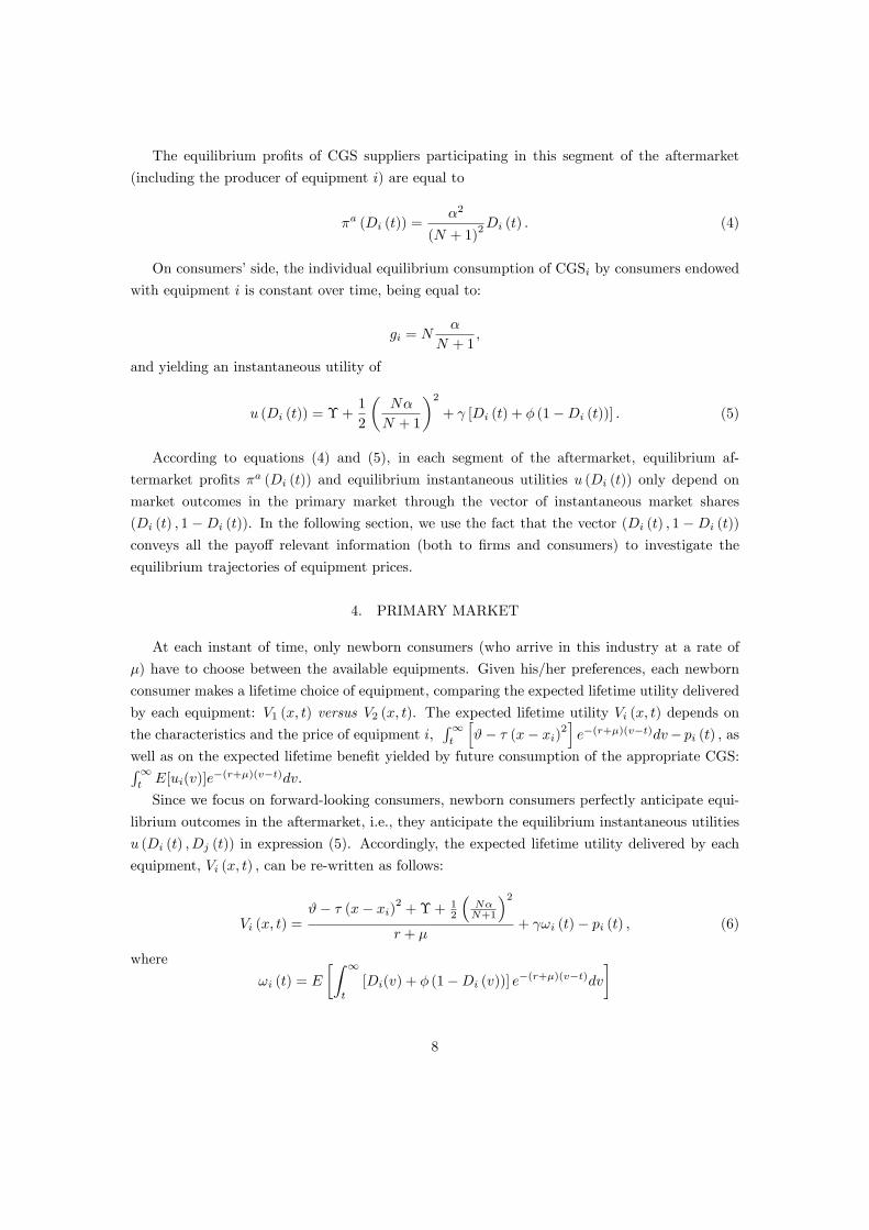
The equilibrium pro�ts of CGS suppliers participating in this segment of the aftermarket
(including the producer of equipment i) are equal to
�a (Di (t)) =�2
(N + 1)2Di (t) : (4)
On consumers�side, the individual equilibrium consumption of CGSi by consumers endowed
with equipment i is constant over time, being equal to:
gi = N�
N + 1;
and yielding an instantaneous utility of
u (Di (t)) = � +1
2
�N�
N + 1
�2+ [Di (t) + � (1�Di (t))] : (5)
According to equations (4) and (5), in each segment of the aftermarket, equilibrium af-
termarket pro�ts �a (Di (t)) and equilibrium instantaneous utilities u (Di (t)) only depend on
market outcomes in the primary market through the vector of instantaneous market shares
(Di (t) ; 1 �Di (t)). In the following section, we use the fact that the vector (Di (t) ; 1 �Di (t))
conveys all the payo¤ relevant information (both to �rms and consumers) to investigate the
equilibrium trajectories of equipment prices.
4. PRIMARY MARKET
At each instant of time; only newborn consumers (who arrive in this industry at a rate of
�) have to choose between the available equipments. Given his/her preferences, each newborn
consumer makes a lifetime choice of equipment, comparing the expected lifetime utility delivered
by each equipment: V1 (x; t) versus V2 (x; t). The expected lifetime utility Vi (x; t) depends on
the characteristics and the price of equipment i;R1t
h#� � (x� xi)2
ie�(r+�)(v�t)dv� pi (t) ; as
well as on the expected lifetime bene�t yielded by future consumption of the appropriate CGS:R1tE[ui(v)]e
�(r+�)(v�t)dv:
Since we focus on forward-looking consumers, newborn consumers perfectly anticipate equi-
librium outcomes in the aftermarket, i.e., they anticipate the equilibrium instantaneous utilities
u (Di (t) ; Dj (t)) in expression (5). Accordingly, the expected lifetime utility delivered by each
equipment, Vi (x; t) ; can be re-written as follows:
Vi (x; t) =#� � (x� xi)2 +�+ 1
2
�N�N+1
�2r + �
+ !i (t)� pi (t) ; (6)
where
!i (t) = E
�Z 1
t
[Di(v) + � (1�Di (v))] e�(r+�)(v�t)dv
�
8
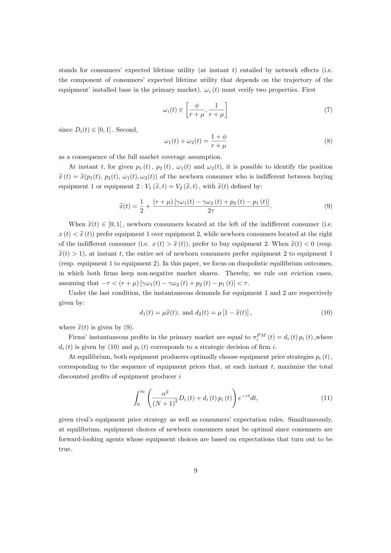
stands for consumers� expected lifetime utility (at instant t) entailed by network e¤ects (i.e.
the component of consumers� expected lifetime utility that depends on the trajectory of the
equipment�installed base in the primary market). !i (t) must verify two properties. First
!i(t) 2�
�
r + �;1
r + �
�(7)
since Di(t) 2 [0; 1] : Second,!1(t) + !2(t) =
1 + �
r + �(8)
as a consequence of the full market coverage assumption.
At instant t; for given p1 (t) ; p2 (t) ; !1(t) and !2(t); it is possible to identify the positionex (t) = ex(p1(t), p2(t), !1(t); !2(t)) of the newborn consumer who is indi¤erent between buyingequipment 1 or equipment 2 : V1 (ex; t) = V2 (ex; t) ; with ex(t) de�ned by:
ex(t) = 1
2+(r + �) [ !1(t)� !2 (t) + p2 (t)� p1 (t)]
2�: (9)
When ex(t) 2 ]0; 1[ ; newborn consumers located at the left of the indi¤erent consumer (i.e.x (t) < ex (t)) prefer equipment 1 over equipment 2; while newborn consumers located at the rightof the indi¤erent consumer (i.e. x (t) > ex (t)), prefer to buy equipment 2: When ex(t) < 0 (resp.ex(t) > 1); at instant t; the entire set of newborn consumers prefer equipment 2 to equipment 1(resp. equipment 1 to equipment 2): In this paper, we focus on duopolistic equilibrium outcomes,
in which both �rms keep non-negative market shares. Thereby, we rule out eviction cases,
assuming that �� < (r + �) [ !1(t)� !2 (t) + p2 (t)� p1 (t)] < �:
Under the last condition, the instantaneous demands for equipment 1 and 2 are respectively
given by:
d1(t) = �ex(t); and d2(t) = � [1� ex(t)] ; (10)
where ex(t) is given by (9).Firms�instantaneous pro�ts in the primary market are equal to �PMi (t) = di (t) pi (t) ;where
di (t) is given by (10) and pi (t) corresponds to a strategic decision of �rm i:
At equilibrium, both equipment producers optimally choose equipment price strategies pi (t) ;
corresponding to the sequence of equipment prices that, at each instant t; maximize the total
discounted pro�ts of equipment producer i
Z 1
0
�2
(N + 1)2Di (t) + di (t) pi (t)
!e�rtdt; (11)
given rival�s equipment price strategy as well as consumers�expectation rules. Simultaneously,
at equilibrium, equipment choices of newborn consumers must be optimal since consumers are
forward-looking agents whose equipment choices are based on expectations that turn out to be
true.
9
Without any further assumption, this dynamic problem has no closed-form solution and it is
not possible to provide general descriptions on �rms�optimal price strategies or consumers�equi-
librium expectation rules. In this context, we focus our analysis on a more restrictive equilibrium
notion: the Linear Markov Perfect Equilibrium (LMPE).
This equilibrium concept introduces two further assumptions in our model. First, we assume
that expectation rules and price strategies follow Markovian processes. In the context of our
model, this constitutes a reasonable assumption since all the payo¤ relevant information is con-
veyed by the state vector (Di (t) ; 1�Di (t)) : Second, both Markovian processes are assumed to
be linear. As far as concerns this assumption, note that our dynamic game corresponds to a
linear-quadratic di¤erential game21 , since: (i) the instantaneous demand for equipment is linear
in the control variables (pi (t) ; pj (t)); (ii) the equation of motion of Di (t) is linear in the state
variable; and (iii) �rms�total pro�ts are quadratic in control variables and linear in the state
variable (see equation (11)). Our di¤erential game being linear-quadratic, it is natural to search
for the simplest strategies that might-solve this category of di¤erential games: the linear strate-
gies. Furthermore, in the context of linear-quadratic games, the best reply to linear strategies is
also linear.
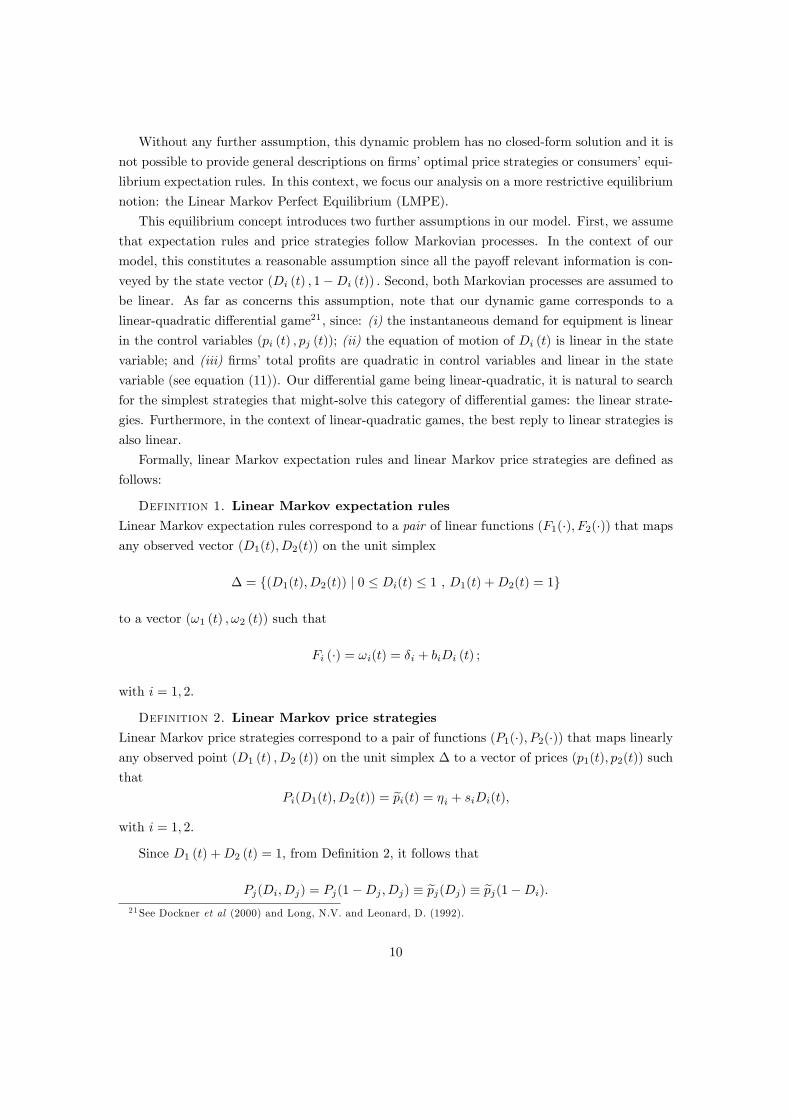
Formally, linear Markov expectation rules and linear Markov price strategies are de�ned as
follows:
Definition 1. Linear Markov expectation rulesLinear Markov expectation rules correspond to a pair of linear functions (F1(�); F2(�)) that mapsany observed vector (D1(t); D2(t)) on the unit simplex
� = f(D1(t); D2(t)) j 0 � Di(t) � 1 , D1(t) +D2(t) = 1g
to a vector (!1 (t) ; !2 (t)) such that
Fi (�) = !i(t) = �i + biDi (t) ;
with i = 1; 2:
Definition 2. Linear Markov price strategiesLinear Markov price strategies correspond to a pair of functions (P1(�); P2(�)) that maps linearlyany observed point (D1 (t) ; D2 (t)) on the unit simplex � to a vector of prices (p1(t); p2(t)) such
that
Pi(D1(t); D2(t)) = epi(t) = �i + siDi(t);
with i = 1; 2:
Since D1 (t) +D2 (t) = 1; from De�nition 2; it follows that
Pj(Di; Dj) = Pj(1�Dj ; Dj) � epj(Dj) � epj(1�Di):
21See Dockner et al (2000) and Long, N.V. and Leonard, D. (1992).
10
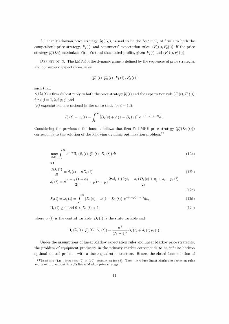
A linear Markovian price strategy, ep�i (Di); is said to be the best reply of �rm i to both the
competitor�s price strategy, Pj(�); and consumers�expectation rules, (F1(�); F2(�)), if the pricestrategy ep�i (Di) maximizes Firm i0s total discounted pro�ts, given Pj(�) and (F1(�); F2(�)):
Definition 3. The LMPE of the dynamic game is de�ned by the sequences of price strategies
and consumers�expectations rules
fep�1 (t) ; ep�2 (t) ; F1 (t) ; F2 (t)gsuch that:
(i) ep�i (t) is �rm i�s best reply to both the price strategy epj(t) and the expectation rule (Fi(t); Fj(:)),for i; j = 1; 2; i 6= j; and
(ii) expectations are rational in the sense that, for i = 1; 2;
Fi (t) = !i(t) =
Z 1
t
[Di(v) + � (1�Di (v))] e�(r+�)(v�t)dv:
Considering the previous de�nitions, it follows that �rm i0s LMPE price strategy (ep�i (Di (t)))
corresponds to the solution of the following dynamic optimization problem:22
maxepi(t)Z 1
0
e�rt�i (epi (t) ; epj (t) ; Di (t)) dt (12a)
s.t.
dDi (t)
dt= di (t)� �Di (t) (12b)
di (t) = �� � (1 + �)
2�+ � (r + �)
2 �i + (2 bi � sj)Di (t) + �j + sj � pi (t)2�
(12c)
Fi(t) = !i (t) =
Z 1
t
[Di(v) + � (1�Di (t))] e�(r+�)(v�t)dv; (12d)
�i (t) � 0 and 0 < Di (t) < 1 (12e)
where pi (t) is the control variable, Di (t) is the state variable and
�i (epi (t) ; epj (t) ; Di (t)) =�2
(N + 1)2Di (t) + di (t) pi (t) :
Under the assumptions of linear Markov expectation rules and linear Markov price strategies,
the problem of equipment producers in the primary market corresponds to an in�nite horizon
optimal control problem with a linear-quadratic structure. Hence, the closed-form solution of
22To obtain (12c), introduce (9) in (10), accounting for (8). Then, introduce linear Markov expectation rulesand take into account �rm j0s linear Markov price strategy.
11
this problem23 can be obtained and it is possible to describe the properties of equilibrium price
strategies.
Lemma 1. Properties of expectation rules and price strategiesIn the duopolistic LMPE of the game:
(i) Linear Markov expectation rules are perfectly symmetric, with:
b1 = b2 = b and �1 = �2 = �;
(ii) Linear Markov price strategies are also perfectly symmetric, with
s1 = s2 = s and �1 = �2 = �:
Proof. see the Appendix.
According to Lemma 1, at equilibrium, linear Markov expectation rules and price strategies
are symmetric. In this context, at equilibrium, instantaneous equipment prices p1 (t) and p2 (t)
only di¤er when there is an asymmetry regarding the size of equipment producers�"installed base
of customers"Di (t) :The same applies, mutatis mutandis, to the linear Markov expectation rules.
The symmetry properties identi�ed in Lemma 1 are brought about by (i) the symmetry of
the primitives of our model and (ii) the exclusive focus on duopolistic outcomes. Concerning the
symmetry of the primitives of the model, note that, equipment are considered to be symmetric
with respect to every characteristic except their initial installed base of consumers. Would one of
the equipment producers have an exogenous advantage over its rival (e.g. a quality advantage24
or a "better location" on the Hotelling line, being closer to the preferences of a larger fraction of
consumers), asymmetric price strategies and expectation rules would be expected at the LMPE.
Concerning the focus on duopolistic outcomes, this assumption rules out the case where the
market tips and therefore, our analysis rules out situations in which the �rm with a larger
installed base of equipment owners (dominant equipment producer) makes use of this exogenous
advantage to evict the rival �rm.
It is worth noting that, even in the context of our model, the symmetric LMPE may not
exist. Proposition 1 identi�es the necessary and su¢ cient conditions for the existence of a
unique LMPE.
Proposition 1. Existence and uniqueness of the LMPEA unique LMPE exists if and only if the intensity of network e¤ects, is su¢ ciently small in
23For theorems stating necessary and su¢ cient conditions, see, for example, Long, N.V. and Leonard,D. (1992),Chapter 9.24See Argenziano (2008) for a model of static price competition in a duopoly with vertical and horizontal
di¤erentiation and network e¤ects.
12
relation to the degree of product di¤erentiation, � :
� � � (3r + 2�)
(1� �) (r + 2�) : (13)
Proof. see the Appendix.
According to Proposition 1; a unique symmetric LMPE exists only when the intensity of
network e¤ects, ; is not too strong in relation to � . When network e¤ects are very strong, �rms
may have incentives to move away from the symmetric price strategies, in order to amplify as
much as possible the network e¤ects created by their installed base of consumers.
The likelihood of ful�lling condition � depends on the remaining parameters of the
model (� ; �; r; �): When equipments are considerably di¤erentiated (� is large) or the degree of
compatibility between network e¤ects is large (� is large); the existence and uniqueness condition
(13) is more likely satis�ed. This is also the case when �rms discount more future pro�ts (r is
large): In contrast, in a scenario of rapid turnaround in the composition of the population of
equipment owners (� is large), it becomes more di¢ cult to ful�ll the existence and uniqueness
condition.
In what follows, we assume that condition (13) is met and we investigate further properties
of equilibrium price strategies.
4.1. LMPE price strategies
Proposition 2. Along the LMPE price trajectories, the equipment with a larger instanta-
neous installed base of consumers is more expensive than the rival equipment:
p�i (t)� p�j (t) = s�[Di (t)�Dj (t)]
with s� > 0:
Proof. See the Appendix.
Proposition 2 puts forward the existence of a "network premium" for equipment producers
enjoying a larger installed base of customers (dominant equipment). When aftermarkets exhibit
network e¤ects, the larger the installed base of consumers endowed with equipment i; the more
valuable CGSi become. Hence, from the perspective of newborn consumers, the dominant equip-
ment has a qualitative advantage over its rival25 . However, when condition (13) is ful�lled, the
producer of the dominant equipment is not interested in adopting aggressive price-cutting strate-
gies in the primary market. Under (13), network e¤ects tend to be relatively weak in relation to
equipment di¤erentiation and, therefore, it is highly unlikely that newborn consumers "located
distantly" from the dominant equipment choose to buy it. The dominant equipment producer
25When taking their equipment decisions, newborn consumers account for this qualitative advantage but theyalso consider the location of equipment on the Hotelling line.
13
acts like a "fat cat"26 , accommodating itself to the rival equipment producer by charging a higher
price for its "superior" equipment27 .
The fat cat e¤ect just described tends to be more signi�cant in a scenario of stronger network
e¤ects ( is larger) or weaker product di¤erentiation (� is smaller), leading to a greater price
di¤erential between the dominant equipment and its rival. In fact from (40) in Appendix, it
follows also that the derivative @s(b�)@b is positive when r > 2�: In these circumstances, the gap
in the instantaneous equipment prices p�i (t) � p�j (t) depends positively on b; which is turn is
determined by the parameters ; � ; r ; � and �. In particular, for r > 2�; it follows that b� is an
increasing function of � for ( ; �) such that condition (13) holds.
Finally, it is worth noting that s� does not depend on N and therefore, the degree of com-
petition in aftermarkets does not a¤ect the equilibrium di¤erential of instantaneous equipment
prices.
Proposition 3. In the LMPE, � (b�) is positively related to the degree of di¤erentiation
between equipment (�) and negatively related with the degree of aftermarkets�pro�tability, which
is determined by the degree of competition in aftermarkets (N), the intrinsic value of CGS (�)
and the relative intensity of network e¤ects� �
�. Depending on the interplay of these elements,
at equilibrium � (b�) Q 0:
Proof. See the Appendix.
In the context of linear Markov price strategies, � corresponds to the component of price that
does not depend on equipment�installed base of customers. At equilibrium:
� (b�) =�
(r + �)(a)
+ �(1� �� b� (r + 2�))
b�2� (r + �)2 (2 (1� �)� b� (r + �))
(b)
� �2
(r + �) (N + 1)2(c)
(14)
From (14); it follows that, in line with Proposition 2; � (b�) is the sum of three terms: (a)
the "Hotelling price"�
�r+�
�, (b) a "lock in discount", and (c) a discount related to the lack
of competition in aftermarkets. The Hotelling price corresponds to the price that would be
charged by equipment producers if they were not involved in the production of CGS. When
equipment producers simultaneously participate in the primary market and the aftermarket,
both equipment producers compete more �ercely for new (lock in) consumers to avoid loosing
pro�ts in the aftermarket28 . The more pro�table are aftermarkets in comparison with primary
markets ( � is larger); the larger is discount (b) in equation (14). In contrast, in the absence
of network e¤ects ( = 0) ; there is no lock in discount since component (b) in equation (14) is
equal to zero.
26We borrow this terminology from Fudenberg and Tirole (1983).27The superiority of the equipment is caused by network e¤ects. The fact that the dominant equipment bene�ts
from a larger installed basis of consumers makes future consumption of the compatible CGS more valuable.28Remind that the pro�ts of each CGS supplier (including equipment producers) are positively correlated with
the number of consumers endowed with the corresponding equipment.
14
In addition, � (b�) depends positively on the intensity of competition in the aftermarket29 .
When competition in aftermarkets is tougher (N is larger), � (b�) is higher and, therefore, both
equipment are more expensive (regardless of their installed base of consumers). At the limit,
when aftermarkets are perfectly competitive, the discount (c) in equation (14) is null. Notice also
that, the increase in equipment price triggered by tougher competition in aftermarkets is greater
the higher the marginal bene�t of CGS consumption (�) and the lower the e¤ective discount
rate (r + �) :
Corollary 1. In the LMPE:
� �2
4 (r + �)� �� � �
r + �:
Proof. See the Appendix.
Corollary 1 de�nes the set of possible values of � (b�) :When there are no network e¤ects and
aftermarkets are perfectly competitive ( = 0 and N !1) ; there is no "lock in discount" nor"lack of competition" discount, and � (b�) = �
r+� : When the intensity of network e¤ects reaches
its upper limit ( ful�lls condition (13) in equality), the "lock in discount" is maximum and it is
equal to �r+� ; yielding �
� = � �2
(N+1)2(r+�)< 0: Accordingly, �� reaches its minimum value when
ful�lls condition (13) in equality and, simultaneously, equipment producers have the monopoly
of CGS provision (N = 1), yielding �� = � �2
4(r+�) :
When aftermarkets are very competitive and/or network e¤ects are relatively strong in rela-
tion to di¤erentiation between equipment, � (b�) can be negative, eventually leading to negative
equipment prices, especially in the case of the dominated equipment producer ("lean and hungry"
e¤ect30).
4.2. LMPE trajectories and Steady state
This subsection analyzes the process of convergence to the steady state LMPE, investigating
the LMPE trajectories of equipment�instantaneous market shares Di (t) and equipment�prices
pi (t) :
By de�nition, in the steady state equilibrium di (t) = �Di (t) ; or equivalently
dDi (t)
dt= 0; (15)
yielding31 Di =12 ;where Di stands for the steady state LMPE market share of equipment
29Section 5 shows that any additional pro�ts on aftermarkets translate into lower pro�ts in the primary market,since equipment producers compete more �ercely to attract newborn consumers.30We borrow this terminology from Fudenberg and Tirole, 1983.31To obtain the steady state market share, in (15), substitute di (t) by the expression (12c). Then, introduce
� =1+��b(r+�)
2(r+�)(see (20)) and account for the linear Markov price strategies of �rm i: Finally, solve equation
(15), obtaining Di =12:
15
producer i; i = 1; 2: Not surprisingly, in the steady state LMPE, equipment producers have
symmetric market shares in the primary market. This result is a direct consequence of the fact
that we focus exclusively on duopolistic equilibrium outcomes within a model where �rms are
symmetric with respect to every characteristic but initial market shares in the primary market.
The producer of the dominant equipment assumes a "fat cat" behavior, charging higher
equipment prices and, accordingly, it becomes increasingly less attractive to new consumers until
the symmetric steady state is reached. Whether this process of market shares convergence is
slower or faster depends on the characteristics of the markets.
Proposition 4. In the LMPE, market shares converge to the symmetric steady state equi-
librium at a rate equal to
=1� �b�
� (r + �):
Proof. See the Appendix.
Corollary 2. In the LMPE, the speed of convergence to the symmetric steady state is such
that 0 � � �:
Proof. Follows directly from Proposition 4 and the fact that 1��r+2� � b� � 1��
r+� :
Proposition 4 states that the speed of convergence to the symmetric steady state depends
on the e¤ective discount rate (r + �), on the degree of compatibility between network e¤ects
and on the equilibrium value of b�; which is determined by the parameters ; � ; �; r and �:
Convergence to the symmetric steady state is slower in industries characterized by weaker product
di¤erentiation (� is smaller) and stronger network e¤ects (larger ): In these circumstances, the
rational expectations on the future market shares are more sensitive to equipment�instantaneous
base of consumers (b� is larger) and the "fat cat" e¤ect tends to be more limited. Accordingly
the equilibrium gap jpi (t)� pj (t)j is also smaller and the asymmetry between �rms�marketshares prevails longer. This result is in line with Doganoglu (2003) and Laussel et al (2004).
It is also worth noting that, as illustrated by Corollary 2; there might be a considerable
degree of inertia in the evolution of equipment market shares. This is more likely to occur when
network e¤ects are stronger (larger ) or product di¤erentiation is weaker. In any case, when
the turnaround in the population of equipment owners is relatively limited (� is small), the
convergence to the steady state LMPE tends to be slower, independently of the preferences of
equipment owners ( ; �; �) :
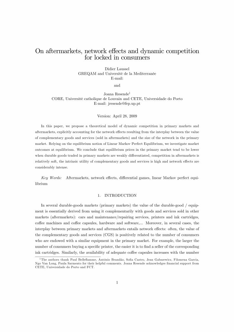
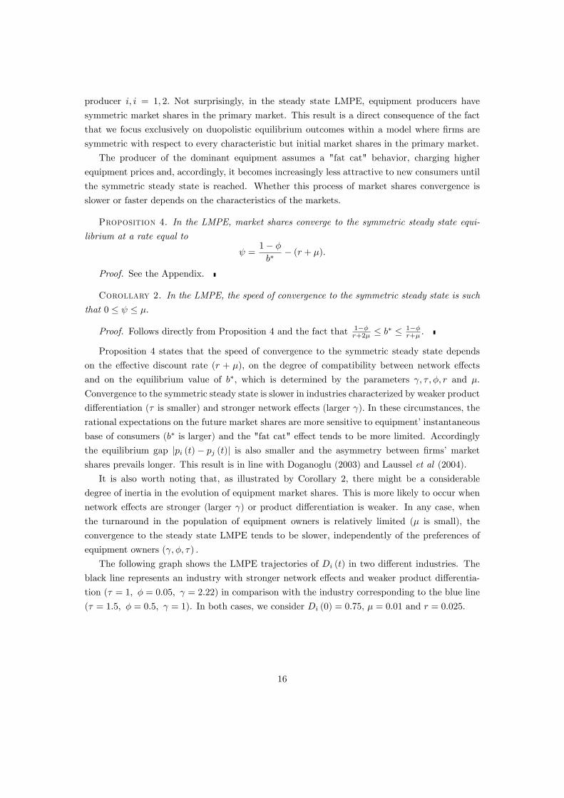
The following graph shows the LMPE trajectories of Di (t) in two di¤erent industries. The
black line represents an industry with stronger network e¤ects and weaker product di¤erentia-
tion (� = 1; � = 0:05; = 2:22) in comparison with the industry corresponding to the blue line
(� = 1:5; � = 0:5; = 1). In both cases, we consider Di (0) = 0:75; � = 0:01 and r = 0:025:
16
0 200 4000.0
0.5
1.0
t
Di(t)
LMPE trajectories of Di (t) ; with Di (0) = 0:75; r = 0:02; � = 0:01
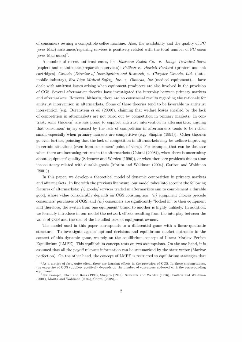
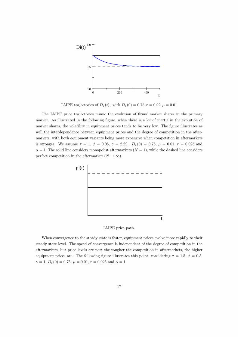
The LMPE price trajectories mimic the evolution of �rms�market shares in the primary
market. As illustrated in the following �gure, when there is a lot of inertia in the evolution of
market shares, the volatility in equipment prices tends to be very low. The �gure illustrates as
well the interdependence between equipment prices and the degree of competition in the after-
markets, with both equipment variants being more expensive when competition in aftermarkets
is stronger. We assume � = 1; � = 0:05; = 2:22; Di (0) = 0:75; � = 0:01; r = 0:025 and
� = 1: The solid line considers monopolist aftermarkets (N = 1), while the dashed line considers
perfect competition in the aftermarket (N !1).
t
pi(t)
LMPE price path.
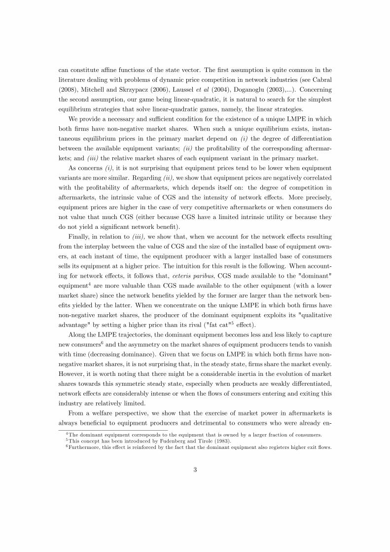
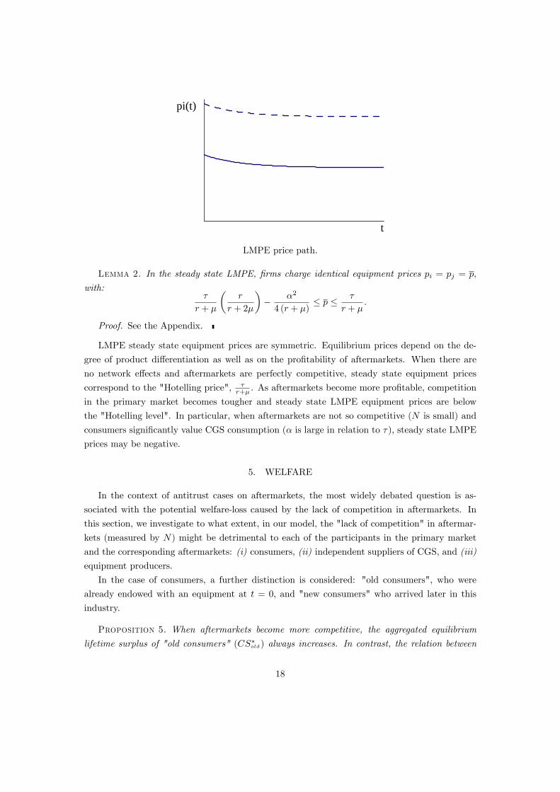
When convergence to the steady state is faster, equipment prices evolve more rapidly to their
steady state level. The speed of convergence is independent of the degree of competition in the
aftermarkets, but price levels are not: the tougher the competition in aftermarkets, the higher
equipment prices are. The following �gure illustrates this point, considering � = 1:5; � = 0:5;
= 1; Di (0) = 0:75; � = 0:01; r = 0:025 and � = 1:
17
t
pi(t)
LMPE price path.
Lemma 2. In the steady state LMPE, �rms charge identical equipment prices pi = pj = p;
with:�
r + �
�r
r + 2�
�� �2
4 (r + �)� p � �
r + �:
Proof. See the Appendix.
LMPE steady state equipment prices are symmetric. Equilibrium prices depend on the de-
gree of product di¤erentiation as well as on the pro�tability of aftermarkets. When there are
no network e¤ects and aftermarkets are perfectly competitive, steady state equipment prices
correspond to the "Hotelling price", �r+� . As aftermarkets become more pro�table, competition
in the primary market becomes tougher and steady state LMPE equipment prices are below
the "Hotelling level". In particular, when aftermarkets are not so competitive (N is small) and
consumers signi�cantly value CGS consumption (� is large in relation to �); steady state LMPE
prices may be negative.
5. WELFARE
In the context of antitrust cases on aftermarkets, the most widely debated question is as-
sociated with the potential welfare-loss caused by the lack of competition in aftermarkets. In
this section, we investigate to what extent, in our model, the "lack of competition" in aftermar-
kets (measured by N) might be detrimental to each of the participants in the primary market
and the corresponding aftermarkets: (i) consumers, (ii) independent suppliers of CGS, and (iii)
equipment producers.
In the case of consumers, a further distinction is considered: "old consumers", who were
already endowed with an equipment at t = 0; and "new consumers" who arrived later in this
industry.
Proposition 5. When aftermarkets become more competitive, the aggregated equilibrium
lifetime surplus of "old consumers" (CS�old) always increases. In contrast, the relation between
18
the degree of competition in aftermarkets (N) and the aggregated equilibrium lifetime surplus of
"new consumers" (CS�new) is non-monotonic. More precisely:
@CS�old
@N=
1
r + �
�2N
(N + 1)3 > 0; (16)
@CS�new
@N=
�
(r + �) r
�2 (N � 2)(N + 1)
3 :
Proof. See the Appendix.
Proposition 5 shows that the lack of competition in aftermarkets is always detrimental to old
consumers. These consumers were already endowed with an equipment and therefore they are
only interested in purchasing CGS, being penalized by the lack of competition in aftermarkets.
In contrast, new consumers are not endowed with an equipment and, before purchasing CGS,
they have to buy the equipment itself. This entails a non-monotonic relation between the degree
of competition in aftermarkets and CS�new :when aftermarkets become more competitive, new
consumers bene�t from cheaper CGS but both equipment become more expensive (see equation
(14)).
Proposition 6. When aftermarkets become more competitive, the aggregated equilibrium
lifetime pro�ts of independent CGS suppliers (��IS) decreases for N > 3; with:
@��IS@N
= ��2 N � 3r (N + 1)
3 : (17)
Proof. See the Appendix.
According to Proposition 6, when competition in aftermarkets becomes very tough, the aggre-
gated equilibrium lifetime pro�ts of independent CGS suppliers are lower, due to the simultaneous
decline of the unit price of CGS and the individual production of each CGS supplier.
Proposition 7. When aftermarkets become more competitive, the aggregated equilibrium
lifetime pro�ts of equipment producers (��EP ) always decreases:
@��EP@N
=�2�2
(N + 1)3(r + �)
< 0: (18)
The previous e¤ect coincides with the e¤ect of N on the aggregated equilibrium lifetime pro�ts
that equipment producers extract from "old consumers".
Proof. See the Appendix.
Proposition 7 shows that the degree of competition in aftermarkets (N) does not a¤ect the
equilibrium lifetime pro�ts yielded by the interactions of equipment producers with the successive
cohorts of new consumers. Since new consumers are not endowed with an equipment, when
19
aftermarkets become more competitive, equipment producers are able to increase equipment
prices to compensate pro�t losses in the respective aftermarket. When aftermarkets become more
competitive, equipment become more expensive (the price discount � �2
(r+�)(N+1)2in equation
(14) becomes smaller), exactly compensating the lifetime pro�t-losses (per new consumer) that
equipment producers su¤er in the aftermarket as a consequence of increasing competition.
From the preceding propositions, it follows that the "lack of competition" in aftermarkets
a¤ects di¤erently the agents involved in this industry. The following Proposition investigates the
e¤ect of N on equilibrium total social welfare ("Marshallian social welfare"):
W � = CS�old + CS�new +�
�IS +�
�EP :
Proposition 8. The lack of competition in aftermarkets has a detrimental e¤ect on total
social welfare, with:@W �
@N=
�2
r (N + 1)3 > 0:
Proof. Follows directly from (16), (17) and (18).
According to Proposition 8; the lack of competition in aftermarkets has a detrimental e¤ect
on total social welfare.
The magnitude of the welfare loss is determined by the characteristics of the aftermarket,
namely the marginal bene�t entailed by CGS consumption�@W�
@N depends positively on ��and
the discount factor�@W�
@N depends negatively on r�:
In line with other models dealing with aftermarket competition (see, for example Shapiro
(1995) and Borenstein et al (2000)), in the context of our model, total social damage corre-
sponds to the sum of the discounted value of the deadweightloss triangles in each segment of
the aftermarket. The lack of competition in aftermarkets increases the price of CGS, reducing
their consumption below the socially desirable level. In the case of the primary market, there
is no welfare detrimental e¤ect, since the price distortions created by the lack of competition in
aftermarkets32 do not a¤ect equipment choices of newborn consumers.
6. CONCLUSION
In this paper, we propose a theoretical model of dynamic competition in primary markets
and aftermarkets. In line with the previous literature, our model encompasses the key elements
to an aftermarket: (i) the complementarity between durable goods and CGS; (ii) the existence
of a time lag between equipment purchases and CGS consumption; and (iii) consumers�lock in.
In addition, our model takes into consideration the network e¤ects resulting from the interplay
between the value of CGS and the market shares of equipment producers.
To investigate strategic interaction between �rms we develop a linear-quadratic di¤erential
32Remind that equipment prices are negatively a¤ected by the degree of competition in aftermarkets.
20
game. In the context of this game, we search for the unique LMPE in which both �rms have
non-negative market shares and we provide a necessary and su¢ cient condition for the existence
of such equilibrium. When the existence and uniqueness condition is ful�lled, we show that, at
equilibrium, instantaneous equipment prices are determined by the interplay of the degree of
di¤erentiation between equipment variants and the pro�tability of aftermarkets, which depends
itself on the on the degree of competition in aftermarkets, on the intrinsic value of CGS and on
the intensity of network e¤ects. Equipment prices tend to be lower when (i) equipment variants
are weakly di¤erentiated, (ii) competition in aftermarkets is relatively soft, (iii) CGS have a
high intrinsic utility, and (iv) network e¤ects are rather intense. Moreover, when e¤ects (i), (ii)
or (iii) are very signi�cant, instantaneous equipment prices may be negative at equilibrium.
In line with the literature on dynamic price competition in network industries, we found
that, at equilibrium, the equipment producer with a larger installed base of consumers quotes a
higher equipment price that re�ects the greater network bene�ts generated in the corresponding
aftermarket (fat cat behavior). The dominant equipment becomes less and less attractive to
newborn consumers and, along the LMPE trajectories, market shares converge to the symmetric
steady state (decreasing dominance). However, when network e¤ects are rather intense in relation
to di¤erentiation between equipment variants, there might be a considerable degree of inertia in
the evolution of market shares. Furthermore, the speed of convergence never exceeds the rate of
consumers�turnaround (entry/exit rate).
From a welfare perspective, we conclude that the social damages entailed by the exercise of
market power in aftermarkets are exclusively related to the underprovision of CGS in aftermar-
kets. Any additional pro�ts on aftermarkets translate into tougher competition in the primary
market, yielding lower equipment prices.
In our future research, we intend to investigate to which extent network e¤ects resulting
from the interplay between primary markets and aftermarkets may lead to eviction outcomes:
when network e¤ects are very strong in relation to product di¤erentiation, equipment producers
may have incentives to adopt aggressive pricing policies in the initial periods, in order to the
evict the rival equipment producer. In our future research, we intend to study in which circum-
stances eviction outcomes may arise at equilibrium, investigating also the corresponding welfare
implications.
We are also interested in extending our model to more complex types of network e¤ects,
evaluating in which circumstances network e¤ects may lead to the "increasing dominance" phe-
nomenon described by Cabral (2008). In particular, we intend to study the case of "multiplicative
network e¤ects", occurring when the size of the network positively e¤ects the marginal bene�t of
CGS consumption. Finally, we also intend to consider asymmetric competition in aftermarkets,
investigating how the intensity of competition in one aftermarket segment may a¤ect market
outcomes in the other aftermarket segment.
Appendix
Proof of Lemma 1
21
The proof is organized as follows. First, we prove that, when consumers are forward-looking,
the assumption of linear Markov expectation rules implies b1 = b2 = b: Then, we show that
s1 = s2 = s for equilibrium price strategies to be compatible with the assumptions of linear
Markov expectation rules and linear Markov price strategies. Finally, at the end of the proof,
we show that �1 = �2 = � and �1 = �2 = �:
Under the assumption of linear Markov expectation rules (De�nition 1), we have that
Fi (�) = �i + biDi (t) = !i (t) : (19)
Considering (8), condition (19) implies �2 + b2D2 (t) =1+�r+� � [�1 + b1D1 (t)], or equivalently
, �2 + b2D2 (t) =1 + �
r + �� �1 � b1 + b1D2 (t) : (20)
From (20), it follows that b1 = b2 = b:
To show that s1 = s2 = s; we introduce the current-value co-state variable �i(t) and we de�ne
the current-value Hamiltonian for �rm i as follows:
Hi(t) = [pi (t) + �i (t)] di (t) + �2 Di (t)
(N + 1)2 � ��i (t)Di (t) ; (21)
where, under linear Markovian expectation rules and linear Markovian price strategies, di (t) is
given by (12c).
The necessary conditions to guarantee optimality of �rm i�s equipment price strategies in-
clude:@Hi(t)
@pi (t)= 0 (22)
andd�i(t)
dt= r�i(t)�
@Hi(t)
@Di(t); (23)
with i = 1; 2:
From the �rst order conditions (22) and (23), we obtain:
�i (t) =� � (1 + �)
r + �+ �j + sj [1�Di(t)]� 2pi (t) + 2 [�i + biDi (t)] ; (24)
and
d�i(t)
dt= (r + �)�i(t)�
� (r + �) (2 bi � sj)2�
[pi (t) + �i (t)]��2
(N + 1)2 ; (25)
with i = 1; 2:
In condition (25), replace �i(t) for the RHS of condition (24) and introduce the linear Markov
price strategy of �rm i; pi = �i+siDi (t) ; obtainingd�i(t)dt = Ai+BiDi(t); where the polynomials
Ai and Bi depend on the parameters of the model as well as on the values of b; �i; �j ; �i; �j ; si
22
and sj : Then, introduce �rm i0s linear Markov price strategy in condition (24) and di¤erentiate
it with respect to time, obtaining
d�i(t)
dt= (2 bi � sj � 2si)
dDi(t)
dt, (26)
where dDi(t)dt is determined by the motion equation. Accounting for the linear Markov price
strategy of �rm i, dDi(t)dt is equal to
�
��� (1+�)+(r+�)[2 �i+(2 bi�sj�si)Di(t)+�j+sj��i]
2� �Di (t)
�:
Introducing this expression in (26) and putting Di (t) on evidence, one obtainsd�i(t)dt =
Fi + GiDi(t);where again Fi and Gi depend on the parameters of the model as well as on the
values of b; �i; �j ; �i; �j ; si and sj :
In the LMPE of the game, it must be the case that, at each instant t � 0, and for i = 1; 2;Ai +Bi Di(t) = Fi +Gi Di(t)8Di (t) : Thus, it follows that Ai = Fi and Bi = Gi; for i = 1; 2:
The condition Bi = Gi implies that:
(r + �)���(�si � sj + 2b )2
�+ (2si + sj � 2b ) (r + 2�) = 0; (27)
for i = 1; 2: Subtracting the second from the �rst, we obtain (s1 � s2) (r + 2�) = 0; which is
consistent with s1 = s2 = s:
To demonstrate that �1 = �2 = �; note that equating Ai and Fi for i = 1; 2; yields two
equations in �1 and �2: Subtracting the second from the �rst, one obtains
(r + �)
�((�1 � �2) (3� + 4s�� 4b �) + 2 (�1 � �2) (�� � 2s�+ 2b �)) = 0: (28)
In addition, given linear Markov expectation rules we have that �i + bDi = !i (t) ; where
!i (t) is given by (12d) since consumers are forward-looking agents. Di¤erentiating both sides of
this equality with respect to time, we obtain
bdDi (t)
dt= (r + �) [�i + bDi(t)]� [Di(t) + �(1�Di(t))] (29)
Replacing in (29) the law of motion dDi(t)dt by the expression derived above and considering
si = sj = s; it follows the condition MDi (t) + Ni = 0; where M is a function of b; s and the
parameters of the model, while Ni is a function of the parameters of the model as well as on the
values of b; s; �i; �j ; �i and �j : Since condition MDi (t) + Ni = 0 must hold for all values of
Di 2 [0; 1], it follows that M = 0, or equivalently
1
2�
�2 b2� (r + �)� 2b (s� (r + �) + � (r + 2�)) + 2� (1� �)
�= 0 (30)
23
It also follows that Ni = 0; yielding
�i =2b�(r + �)(�i � �j) + 2 b�(1 + �)� 2b�� � 4��� 2bs�(r + �)
2(r + �)(2 b�� 2�) ; (31)
for i = 1; 2: Subtracting �2 from �1, we obtain:
�1 � �2 = b��1 � �2b �� � : (32)
Replacing condition (32) in equation (28), we obtain (r + �) (�1 � �2) 5b ��3��4s�b ��� = 0; which
is consistent with �1 = �2 = �:
Finally, given that �1 = �2 = �; equation (32) yields �1 = �2 = �:�
Proof of Proposition 1The proof is organized as follows. First, we use equilibrium conditions (27) and (30) to express
the b � value at the LMPE equilibrium as a function of the parameters of the model. Then
we investigate the existence of further constraints on the equilibrium b � value imposed by the
hypothesis of rational expectations together with the assumptions of linear Markov expectations.
To start, solve equation (30) with respect to s; obtaining s (b) equal to:
s (b) =2 b2�(r + �) + 2�(1� �� b(r + 2�))
2b�(r + �): (33)
Then, in condition (27) consider s1 = s2 = s and replace s for its value in equation (33), obtaining
the LMPE equilibrium condition that implicitly expresses b� as a function of the parameters of
the model:
�� (r + �) (r + 2�) b�3 + (r + 2�)
2b�2 � 5 (1� �) (r + 2�) b� + 4 (�� 1)2 = 0; (34)
However, note that, not all the values of b that solve (41) constitute a LMPE. In particular,
rational expectations, together with the assumptions of linear Markov expectation rules impose
the following additional restrictions:
0 < b� � 1� �r + �
: (35)
To obtain that b� > 0; notice that equation (29) corresponds to a di¤erential equation. Upon
integration, we get:
Di (v) = K + (Di (t)�K) e(r+�)b�(1��)
b (v�t); (36)
with K = �(r+�)��(1��)�b(r+�)
Finally, substituting (36) in the RHS of (12d), we obtain:
!i (t) =�(1��)�b�
(1��)�b(r+�) + (1� �) (Di (t)�K)R1te�
(1��)b (v�t)dv:
24
The previous expression can only be equal to F (�) = � + bDi (t) if b is strictly positive.
Regarding the condition b � 1��r+� ; notice that condition (7) requires:
�
r + �� � + bDi (t) �
1
r + �8 Di (t) 2 [0; 1]: (37)
In particular, for Di = 0; condition (37) implies �r+� � � � 1
r+� : Similarly, for Di = 1;
condition (37) implies �r+� � b � � � 1
r+� � b: Therefore
�
r + �� � � 1
r + �� b: (38)
To guarantee that the set of ��values in (38) is non-empty, b must be small enough. Moreprecisely b � 1��
r+� :
In this context, the LMPE value of b� correspond to the root(s) of the cubic polynomial in
(34) that are included in the interval 0 < b� � 1��r+� :
To conclude the proof, we investigate under which conditions the polynomial in condition
(34), hereafter denoted by X (b) has only one root such that b� 2�0; 1��r+�
i. In this case, the
LMPE exists and it is unique.
To start, notice that X (b) is a third-degree polynomial and it has, at most, three roots.
Given that X (�1) = �1 and X (0) = 4� (�� 1)2 > 0; one of the roots of X (b) is necessarilynegative, violating condition (35). Hence, at most two roots verify condition (35). It is worth
noting that
X�1��r+�
�= �(��1)2(��(3r+2�)� (��1)(r+2�))
(r+�)2Q 0;
and X (+1) = +1: Therefore, a su¢ cient and necessary condition for the existence of aunique root of X (b) satisfying condition (35) is X
�1��r+�
�� 0; or equivalently � �(3r+2�)
(1��)(r+2�) :
When X�1��r+�
�> 0, either the polynomial X (b) has two roots in the interval
�0; 1��r+�
i; or it
has no root in this interval. Thus, condition (13) is a necessary and su¢ cient condition for the
existence of a unique LMPE.�
Proof of Proposition 2The equilibrium value of s is jointly determined by equilibrium conditions (27) and (30).
First, we solve condition (30) with respect to s; obtaining s(b) in equation (33). Then, we solve
the equilibrium condition (34) for ; obtaining
= � (4 (1� �)� b� (r + 2�)) b� (r + 2�)� (1� �)b�3� (r + �) (r + 2�)
; (39)
where b� denotes the equilibrium value of b: Introducing (39) in (33), we obtain the equilibrium
25
value of s conditional on b� :
s (b�) = 2� ((1� �)� b� (r + 2�)) b� (r + 2�)� 2 (1� �)b�2� (r + �) (r + 2�)
(40)
Concerning the sign of s (b�) ; it follows that s (b�) > 0: To show that, at equilibrium s (b�)
must be strictly positive, note that b� � 1��r+� and therefore
b�(r+2�)�2(1��)b�2�(r+�)(r+2�) < 0: Furthermore,
at equilibrium it must be the case that b� > 1��r+2� and therefore 2� ((1� �)� b
� (r + 2�)) < 0:
To verify that b� > 1��r+2� note that X
�1��r+2�
�= � (1� �)3 r+�
(r+2�)2> 0 . Therefore when the
existence and uniqueness condition (13) is met, it must be the case that the unique LMPE is
obtained for 1��r+2� < b� < 1��
r+� :�
Proof of Proposition 3In the Proof of Lemma 1, from (24) and (25) it has been derived the equilibrium condition
Ai = Fi, i = 2: Solving this condition for �; after introducing in condition Ai = Fi the equilibrium
requirement of symmetry regarding expectation rules and price strategies, we obtain
� (b; �; s) =
�� � (1 + �)(r + �)
+ s+ 2 �
��1 + 2
�
�(s� b )
�� �2
(r + �) (N + 1)2 : (41)
Furthermore, analyzing condition (20) in the Proof of Lemma 1 in the light of the symmetry
equilibrium requirement, it follows that � = 1+��b(r+�)2(r+�) : Introducing this condition and condition
(33) in (41), we get (14).
The sign of � (b�) is a priori indeterminate. The term� �2
(r+�)(N+1)2is negative, while the term
� [b� (r + 3�)� 2 (1� �)] b�(r+�)�(1��)(b�)2�(r+�)2
is necessarily positive for b� < 1��r+� given the assumption
� < r2 :�
Proof of Corollary 1From (14) it follows that
d� (b�)
db= � (1� �) b
� (3r + 5�)� 4 (1� �)(b�)
3� (r + �)
2 ;
which is negative given the assumption � > r2 and the result b
� < 1��r+� :
Furthermore,d� (b�)
dN=
2�2
(r + �) (N + 1)3 > 0:
Accordingly, the highest value of � (b�) occurs for b� ! 1��r+2� and N ! 1; yielding �� = �
r+� .
Conversely, the lowest value of � (b�) occurs for b� ! 1��r+� and N = 1; yielding � (b�) = � �2
4(r+�) :�
Proof of Proposition 4Consider the motion law dDi(t)
dt = di (t)��Di (t) : Then, substitute di (t) by expression (12c),
after introducing � = 1+��b(r+�)2(r+�) (see (20)), accounting for the linear Markov price strategies of
26
�rm i and substituting s for expression (33): The resulting expression is a �rst-order di¤erential
equation, whose close solution is given by
Di (t) =1
2+
�Di (0)�
1
2
�e�(
1��b �(r+�))t
and the speed of convergence is equal to�1��b � (r + �)
�:�
Proof of Lemma 2In the steady state LMPE, �rms share the equipment market evenly and, therefore, price
equipment is given by �i +si2 : Considering the equilibrium values of �� and s�; one obtains
p =�
r + �� 2� (1� �) b
� (r + 2�)� (1� �)b�2 (r + 2�) (r + �)
2 ��2
(r + �) (N + 1)2 ; (42)
which depends positively on N and negatively on b�: Evaluating (42) for b� = 1��r+� and N = 1;
we obtain p = �r+�
�r
r+2�
�� �2
4(r+�) : Evaluating (42) for b� = 1��
r+2� and N ! 1; we obtainp = �
r+� :�
Proof of Proposition 5Concerning the aggregated life-time equilibrium surplus of "old consumers" , note that, at
equilibrium, the expected lifetime utility delivered by equipment i to an old consumer located at
x is equal to
#� � (x� xi)2 +�+ 12
�N�N+1
�2r + �
+ !�i (t) ;
since this consumer is already endowed with an equipment. Given that !�i (t) does not depend on
N , the e¤ect of N on the expected life-utility of any "old consumer" is always equal to 1r+�
N�2
(N+1)3
independently of the equipment version owned by this consumer. Since there is a unit mass of
"old consumers", the derivative@CS�old@N is equal to 1
r+�N�2
(N+1)3; which is always positive.
Concerning new consumers, consider the mass � of newborn consumers at instant t:At equi-
librium, the indi¤erent newborn consumer is located at
ex� (t) = 1
2+(r + �) (2D1 (t)� 1) (�s� + b� )
2�; (43)
which is independent of N; given that neither Di (t) ; s� nor b� depend on N: At equilibrium,
the lifetime bene�t of consumers arriving in the market at instant t is equal to
�
Z ex�(t)0
V �1 (x; t) dx+
Z 1
ex�(t) V�2 (x; t) dx
!;
with ex� (t) being given by (43) and Vi (x; t) given by (6) evaluated at equilibrium. Since ex� (t)does not depend on the degree of competition in aftermarkets, the impact of N on the lifetime
27
surplus of consumers arriving in this industry at instant t is equal to
��R ex�(t)
0@V1(x;t)@N dx+
R 1ex�(t) @V2(x;t)@N dx�:
From (6), it follows that @Vi(x;t)@N = �2(N�2)
(N+1)3(r+�)and therefore the e¤ect of N on the lifetime
surplus of consumers arriving in this industry at instant t is equal to � �2(N�2)(N+1)3(r+�)
: Considering
that, in our in�nite horizon model, there is an in�ow of newborn consumers at each instant of
time t � 0; the e¤ect of N on the discounted lifetime surplus of all "new consumers" is equal toZ 1
0
��2 (N � 2)
(N + 1)3(r + �)
e�rtdt =�
r
�2 (N � 2)(N + 1)
3(r + �)
; (44)
which is non-negative for N � 2 and negative otherwise.�
Proof of Proposition 6At equilibrium, aggregated instantaneous pro�ts of independent CGS suppliers participat-
ing in aftermarket i are equal to (N�1)�2(N+1)2
Di(t). Aggregating equilibrium instantaneous prof-
its of all independent CGS suppliers (in both aftermarkets), we obtain (N�1)�2(N+1)2
; given that
D1 (t) +D2 (t) = 1: Therefore, the aggregated equilibrium lifetime pro�ts of independent CGS
suppliers (��is) is given byR10
(N�1)�2(N+1)2
e�rtdt; which is equal to (N�1)�2r(N+1)2
: Accordingly, @��is
@N =
��2 N�3r(N+1)3
:�
Proof of Proposition 7Aggregated equilibrium lifetime pro�ts of equipment producers (��EP ) can be decomposed on
two components: (i) the aggregated pro�ts that equipment producers extract from old consumers,
and (ii) the aggregated pro�ts that equipment producers extract from new consumers.
Equilibrium lifetime pro�ts that equipment producer i extracts from old consumers are given
byR10
�2
(N+1)2Di(0)e
�(r+�)t; that is equivalent to Di(0)(r+�)
�2
(N+1)2: Accordingly, the aggregated equi-
librium lifetime pro�ts that both equipment producers extract from old consumers are equal to1
(r+�)�2
(N+1)2, with @
@N
�1
(r+�)�2
(N+1)2
�equal to �2�2
(r+�)(N+1)3< 0:
Concerning equilibrium lifetime pro�ts that equipment producer i extracts from "new con-
sumers", in addition to pro�ts from CGS, we have to consider pro�ts yielded by equipment sales.
The equilibrium lifetime pro�ts that equipment producer i obtains from selling CGS to new
consumers are given byZ 1
0
�2
(N + 1)2Di(t)e
�rt � 1
(r + �)
�2
(N + 1)2Di(0):
Di¤erentiating this expression with respect to N; we obtain:
�2�2
(N + 1)3
�1� �� b� (r + �)2r (1� �� b��) +
b� (r + 2�)� (1� �)(1� �� b��) (r + �)Di (0)
�< 0: (45)
28
In the primary market, equilibrium instantaneous pro�ts that equipment producer i obtains
from selling equipment to the successive cohorts of "new consumers" are equal to p�i (t) d�i (t) :Hence,
at equilibrium, the lifetime pro�ts that equipment producer i obtains from equipment sales are
equal to: Z 1
0
�� (�� + b�Di (t))
�1
2+(r + �) (2Di (t)� 1) (�s� + b� )
2�
��e�rtdt: (46)
In the previous equation, only �� depends on the degree of competition in aftermarkets.
Replacing s� by expression (33), and considering the equilibrium path of Di (t) ; it follows that
the in�uence of N on (46) is given by
2�2
(N + 1)3
�1� �� b� (r + �)2r (1� �� b��) +
b� (r + 2�)� (1� �)(1� �� b��) (r + �)Di (0)
�> 0;
which is symmetric to (45). As a consequence N does not have any e¤ect on the equilibrium
lifetime pro�ts that equipment producer i extracts from new consumers. Accordingly, the e¤ect
of N on equilibrium lifetime pro�ts of equipment producer i is given by �2�2(r+�)(N+1)3
Di (0) and
the e¤ect of N on the aggregated equilibrium lifetime pro�ts of both equipment producers is
equal to �2�2(r+�)(N+1)3
; which is always negative.�
REFERENCES
[1] Argenziano, R., 2008. "Di¤erentiated networks: equilibrium and e¢ ciency," RAND Journal
of Economics, 39(3), 747-769.
[2] Borenstein,S., Mackie-Mason, J.K. and Netz, J.S., 2000. "Exercising Market Power in Pro-
prietary Aftermarkets," Journal of Economics & Management Strategy, 9(2), 157-188.
[3] Cabral, L., 2007. "Dynamic Price Competition with Network E¤ects," mimeo Portuguese
Competition Authority.
[4] Cabral, L., 2008, "Aftermarket Power and Basic Market Competition," CEPR Discussion
Papers 6802.
[5] Carlton, D.W. and Waldman, M., 2001. "Competition, Monopoly, and Aftermarkets,"
NBER Working Papers 8086.
[6] Chen, Z. and T. Ross, T., 1993. "Refusals to deal, Price Discrimination and Independent
Service Organizations," Journal of Economics & Management Strategy, 2(4), 593-614.
[7] Chen, Z., W. Thomas and W. Stanbury (1998). "Refusals to Deal and Aftermarkets," Review
of Industrial Organization 13, (1-2), 131-151.
29
[8] d�Aspremont, C, Gabszewicz, J.J and J. Thisse, 1979, On Hotelling�s Stability in Compe-
tition, Econometrica 17, 1145-1151.
[9] Dockner, E., S.Jorgensen, N. V. Long, and G., 2000, "Di¤erential Games in Economics and
Management Science," Cambridge University Press, New York.
[10] Doganoglu, T. , 2003, "Dynamic Competition with Consumption Externalities," Netnomics,
5(1), 16-35.
[11] Farrell, J. and Shapiro, C., 1988, "Dynamic competition with switching costs," RAND
Journal of Economics, 19(1), 123- 137.
[12] Fudenberg, D. and J. Tirole, 1991, "Game Theory," MIT Press, Cambridge, MA.
[13] Fudenberg, D. and Tirole, J. 1983, "The fat-cat e¤ect, the puppy-dog ploy, and the lean
and hungry look," American Economic Review, 74, 361� 366.
[14] Klemperer, P., 1987, �Markets with Consumer Switching Costs,�Quarterly Journal of Eco-
nomics, 102, 375-394.
[15] Laussel, D., Montmarin, M. and N. V. Long, 2004, "Dynamic duopoly with congestion
e¤ects," International Journal of Industrial Organization, 22(5), 655-677.
[16] Long, N. V. and D. Leonard, 1992, "Optimal Control Theory and Static Optimization in
Economics," Cambridge University Press.
[17] Maskin, E. and Tirole, J., 2001. "Markov Perfect Equilibrium: I. Observable Actions,"
Journal of Economic Theory, 100(2), 191-219.
[18] Mitchell, M and A. Skrzypacz, 2006, "Network externalities and long-run market shares,"
Economic Theory 29 (3), 621-648.
[19] Morita, H. and Waldman, M., 2004, "Durable Goods, Monopoly Maintenance, and Time
Inconsistency," Journal of Economics and Management Strategy, 13 (2), 273-302.
[20] Schwartz, M and Werden, G. J., 1996, "A Quality-Signaling Rationale for Aftermarket
Tying," Antitrust Law Journal, 64, 387-404.
[21] Shapiro, C., 1995, �Aftermarkets and ConsumerWelfare: Making Sense of Kodak,�Antitrust
Law Journal, 63, 483-511.
30