On accurate differential measurements with electrochemical ... · On accurate differential measurements with electrochemical impedance spectroscopy S.Kernbach, I.Kuksin, O.Kernbach

On accurate differential measurements withelectrochemical impedance spectroscopy

S.Kernbach, I.Kuksin, O.Kernbach

Cybertronica Research, Research Center of Advanced Robotics and Environmental Science,Melunerstr. 40, 70569 Stuttgart, [email protected], [email protected], [email protected]

Abstract—This paper describes the impedance spectroscopyadapted for analysis of small electrochemical changes in fluids.To increase accuracy of measurements the differential approachwith temperature stabilization of fluid samples and electronicsis used. The impedance analysis is performed by the singlepoint DFT, signal correlation, calculation of RMS amplitudesand interference phase shift. For test purposes the samples ofliquids and colloids are treated by fully shielded electromagneticgenerators and passive cone-shaped structures. Fluidic samplescollected from different geological locations are also analysed. Inall tested cases we obtained different results for impacted andnon-impacted samples, moreover, a degradation of electrochem-ical stability after treatment is observed. This method is usedin laboratory analysis of weak emissions and ensures a highrepeatability of results.

I. INTRODUCTION

Electrochemical impedance spectroscopy (EIS) is a commonlaboratory technique in analytical chemistry [1], in biolog-ical research [2], for example, in the analysis of DNA orstructure of tissues, the analysis of surface properties andcontrol of materials [3]. This method consists in applyinga small AC voltage into a test system and registering aflowing current. Based on the voltage and current ratios, theelectrical impedance Z(f) for a harmonic signal of frequencyf is calculated. Measured data are fitted to the model ofconsidered system and allow identifying a number of physicaland chemical parameters.

There are several electrochemical models for EIS. In anumber of publications (e.g. [1]) a current flowing through theelectrode surface is described by the electrochemical reaction

O + ne− → R, (1)

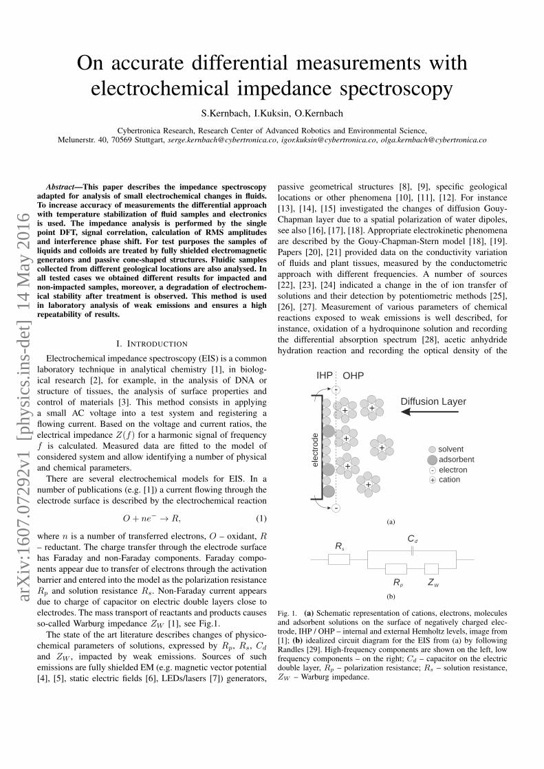
where n is a number of transferred electrons, O – oxidant, R– reductant. The charge transfer through the electrode surfacehas Faraday and non-Faraday components. Faraday compo-nents appear due to transfer of electrons through the activationbarrier and entered into the model as the polarization resistanceRp and solution resistance Rs. Non-Faraday current appearsdue to charge of capacitor on electric double layers close toelectrodes. The mass transport of reactants and products causesso-called Warburg impedance ZW [1], see Fig.1.

The state of the art literature describes changes of physico-chemical parameters of solutions, expressed by Rp, Rs, Cdand ZW , impacted by weak emissions. Sources of suchemissions are fully shielded EM (e.g. magnetic vector potential[4], [5], static electric fields [6], LEDs/lasers [7]) generators,

passive geometrical structures [8], [9], specific geologicallocations or other phenomena [10], [11], [12]. For instance[13], [14], [15] investigated the changes of diffusion Gouy-Chapman layer due to a spatial polarization of water dipoles,see also [16], [17], [18]. Appropriate electrokinetic phenomenaare described by the Gouy-Chapman-Stern model [18], [19].Papers [20], [21] provided data on the conductivity variationof fluids and plant tissues, measured by the conductometricapproach with different frequencies. A number of sources[22], [23], [24] indicated a change in the of ion transfer ofsolutions and their detection by potentiometric methods [25],[26], [27]. Measurement of various parameters of chemicalreactions exposed to weak emissions is well described, forinstance, oxidation of a hydroquinone solution and recordingthe differential absorption spectrum [28], acetic anhydridehydration reaction and recording the optical density of the

+ +

+

+

solvent

electroncation

adsorbent

IHP OHP

Diffusion Layer

+

+

+

-

-

-

ele

ctro

de

(a)

R

R Z

C

W

d

s

p

(b)

Fig. 1. (a) Schematic representation of cations, electrons, moleculesand adsorbent solutions on the surface of negatively charged elec-trode, IHP / OHP – internal and external Hemholtz levels, image from[1]; (b) idealized circuit diagram for the EIS from (a) by followingRandles [29]. High-frequency components are shown on the left, lowfrequency components – on the right; Cd – capacitor on the electricdouble layer, Rp – polarization resistance; Rs – solution resistance,ZW – Warburg impedance.

arX

iv:1

607.

0729

2v1

[ph

ysic

s.in

s-de

t] 1

4 M

ay 2

016

2

solution [30], VIS-UV spectroscopy of the acid-base bromoth-ymol indicator and the salt solution SnCl2 [9].

Performing multiple measurements of weak emissions byconductometric and potentiometric methods [7], [26], [27],we discovered a certain specificity of these measurements.In particular this concerns very small changes of measuredvalues, a high impact of environmental factors, primarily tem-perature and appearance of phenomena that are not observed inother areas. These works lead to development of new sensitivemeasuring devices with differential circuits, ultra-low noise,and thermal stabilization of electronics and samples.

In this paper we describe an adapted EIS approach appliedto several test systems. Two different EIS-meters are used. Thefirst one is the developed differential EIS-meter with phase-amplitude detection of excitation and response signals, thefrequency response is analyzed by a single point DFT andcorrelation analysis. This system is implemented in hardwarein the system-on-chip. The second impedance spectrometeris based on the AD5933 chips from Analog Devices andis used as a control device. It supports only DFT withthe Hanning window function. Experiments have shown thatchanges in samples exposed by weak emissions from fullyshielded EM generators, passive geometrical structures andgeobiological factors are characterized by four values: thedifferential signal amplitude (this value is included in allamplitude characteristics obtained by the frequency responseanalysis); the interference phase shift; ratio between imaginaryand real parts of the impedance (as shown e.g. by the Nyquistplot) and a variation of electrochemical stationary of samples.It is assumed that these parameters can indicate changes innear-electrode layers and diffusion processes in the Randleselectrochemical model [29]. EIS allows analyzing variousliquid and colloidal system and, as an example, we performanalysis of bottled water and milk. Since this work has anexplorative character, we do not intend to collect staticallysignificant data for a particular system – this represents a taskfor further works.

This paper has the following structure. The section II brieflydescribes background of EIS, systematic and random errorsand used devices. Sections III and IV consider the obtainedresults and draw conclusions from these measurements.

II. IMPEDANCE MEASUREMENT, ERRORS ANDDESCRIPTION OF THE DEVICE

There exists an extensive literature on the EIS, both fortheory and models, and for technical aspects of measurements.One of the most common methods for measuring impedancesis related to an auto-balancing bridge [31], where a testsystem is excited by the voltage VV . The flowing current Iis converted into a voltage VI by a transimpedance amplifier(TIA). There are several ways how the signals VI and VV aredigitized and processed in further analysis.

A common approach consists in analyzing the frequencyresponse (frequency response analysis – FRA) of the VI signal,which is based on the discrete Fourier transform (DFT) [32]and synthesis of ideal frequencies. This method is sometimescalled as the single point DFT [33], [34] and requires a fast

ADC with 1 msps and more for digitizing the signal VI . Thedigitized time signal VI(k) with N samples is converted to afrequency signal F (f), containing real Fr(f) and imaginaryFi(f) parts:

Fr(f)+iFi(f) =1

N

N−1∑k=0

VI(k)

[cos(

2πfk

N)− i sin(

2πfk

N)

].

(2)It is common to replace ω = 2πf and to skip 1

N , howeverthese parameters are important for calculating the period [35].The magnitude M(f) and phase P (f) are calculated as:

M(f) =√Fr(f)2 + Fi(f)2, P (f) = tan−1(Fi(f)/Fr(f)).

(3)Calculation of (3) is repeated for all f between minimal fminand maximal fmax frequencies with the step ∆f . DFT andFRA differ in the way how basic vectors cos() and sin() arecalculated. In the FRA they are synthesized (for example thesine, see [34]):

u(f) = A sin(2πg(f)f), g(f) =fmax − fmin

tdur+fmin, (4)

where A is the maximal amplitude, tdur – the duration ofthe measurement, 0 < t < tdur. The synthesized frequencyof base vectors must exactly coincide with the frequency ofmeasured signal. In a sense, the expression (2) calculates acorrelation between ideal and measured signals. If VV and VIare digitized strictly at the same time points, for example, byusing two synchronous ADCs, and since VV is a sine/cosinesignal, (2) takes the form of correlation between V fV and V fI(defined for the frequency f )

Corr(f) =1

N

N−1∑k=0

V fI (k)V fV (k). (5)

Expression (5) is more preferable because here a non-harmonicsignal of high frequency can be used for synthesizing the VV .

The literature discusses non-harmonic signals for driving theelectrochemical system, for example, [36], [37] used digitalsquare waves. An excitation by a broadband noise signal isutilized for a fast impedance spectroscopy [38]. The analysiscan be carried out with a direct amplitude and phase detection.For instance, the maximal or RMS amplitude of VI as well as aphase shift between VV and VI can be calculated without FRA.In more complex cases, the Laplace transform is performedbetween VV and VI .

If the magnitude or the RMS amplitude of VV and VI areknown, the impedance Z for the auto-balancing method isdefined as

Z(f) = rk(f)RTIAVV (f)

VI(f), (6)

where RTIA is a reference resistor in TIA, rk(f) is afrequency-dependent gain caused by analog circuits, inaccu-racies in discrete elements, etc. [31]. Thus, Z is inverselyproportional to VI .

Performing measurements, we found an interesting effect ofchanging the phase of differential signal (VV−VI), as shown inFigs. 11(b), 14(b). This unexpected result is not shown by thephase analysis with FRA (3). This phase variation is created by

3

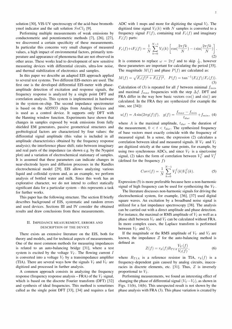
a combination of two factors: the use of direct digital synthesis(DDS) with a low number of samples and application of thedigital infinite impulse response filter (IIR filter):

yn = axn + (1− a)yn−1 = yn−1 + a(xn − yn−1), (7)

where xn are discrete samples of an input signal, yn is thefiltered signal, a is a coefficient. Figure 2 shows the use ofa filter for one period of DDS signal with 40 samples andthe frequency spectrum up to 10 kHz. Such DDS synthesis

200

400

600

800

1000

1200

1400

1600

1800

2000

0 50 100 150 200 250

AD

C V

alu

es

Samples

Phase shift after low pass filter

a=0.5 DAC signal

ADC signal

a=0.1

(a)

a=0.5

a=0.05, impacted

a=0.05, unimpacted

-1

0

1

2

3

4

5

6

7

8

2000 3000 4000 5000 6000 7000 8000 9000 10000

Ph

ase

diff

ere

nce

, S

am

ple

s

Frequency, Hz

Direct Measurement, Phase Spectrum

(b)

Fig. 2. The effect of phase variation after applying the digital IIRfilter (7) with a = 0.5, a = 0.1 and a = 0.05 for a DDS signalsynthesis with a small number of samples for (a) one signal periodwith 40 samples, 3 kHz; (b) the frequency spectrum up to 10 kHz.

includes high frequency components (up to 400-600 kHz)in a low frequency signal. Both low- and high-frequencycomponents impact the samples, this is similar to using abroadband noise for a fast spectroscopy [38]. The IIR filter ata < 0.5 increases the delayed term yn−1, however it appearsdifferently at different frequencies. Thus, we assume that themain reason for the periodic phase shift is an interference withthe high-frequency components in the DDS signal. Hereinafter,this parameter will be referred to as an interference phaseshift Φ. Treatment of samples modifies the response to highfrequency components, which is manifested as a variation ofΦ. With increasing the frequency, this effect decreases, weobserve also a smaller variation of Φ(f).

As emphasized in [1], FRA can only be used for stableand reversible systems in dynamic equilibrium, thereby thelinearity and stability of electrochemical system should beprovided. These are so-called steady-state conditions, wherebydeviations from them can appear, for example, in the formof long transient processes. The stationarity is usually not

investigated by impedance spectroscopy, but it can representan additional source of information about the electrochemicalprocesses before and after the treatment of samples.

The measurement approach for weak emissions is describedin [27], [39], [26]. It uses two identical channel A (ex-perimental) and B (control), which apply the same excitingsignal VV . Spectrograms A and B are subtracted from eachother, the resulting difference spectrum is close to zero atall frequencies if the samples A and B are equal. A non-zero differential spectrum indicates differences in samples.Since both samples are prepared at the same temperature,in the same EM, light and other conditions, the differenceis caused only by exposure to experimental factors. Thismethod requires at least two measurements. In the first onethe samples A and B are measured before impact, these dataare used for calibration. The second measurement of A and Bis performed after exposing the sample A. The measurementresult consists of two differential curves: the calibration (closeto zero) and experimental ones. The difference between themallows making conclusions about impact on the sample A.

A. The error analysis

EIS has several systematic and random errors. The firstsystematic error is related to the period and phase of synthe-sized base vectors and measured signal. The period of signalsaccumulated in arrays VV and VI must be expressed by aninteger. If this condition is not met, so-called leakage errorsoccur. This problem is solved in three ways [35]. Firstly, it isproposed to select the sweep frequencies f in such a way thatVI always contains an integer number of period k. The paper[33] considered a choice of f based on

Ts = k227

fMCLK4

, (8)

where Ts is the digitization time, MCLK is the fundamentalfrequency of AD5933 ([33] is written in the context of thisscheme). The obvious drawback of this approach is that thefrequency step ∆f is large and it is impossible to perform adetailed frequency scan of the test system.

The second method is based on adapting the number ofsamplings N at each sweep. The number of samples N in VIis changed to N0 in (2) so that exactly one period of VI isstored at each reading:

F (f,N0) =1

N0

N0∑k=0

VI(k)e−i2πfkN0 . (9)

Since the base vectors at FRA must have the same frequencyas VI , which is a response to the excitation signal sin() in VV(written as sinVI ()), this leads to

F (f,N0) =1

N0

N0∑k=0

sinVI (2πfk

N0)e−i2π

fkN0 (10)

or components-wise, e.g. for the real part of Fr

Fr(f,N0) =1

N0

N0∑k=0

sinVI (2πfk

N0) cos(2π

fk

N0). (11)

4

Since we record only one period of signal, N0 = f(f) is validfor all frequencies and the main variation of Fr(f(f)) occursdue to N0

Fr(f(f)) =1

f(f)

f(f)∑k=0

sinVI (2πk

N0) cos(2π

k

N0). (12)

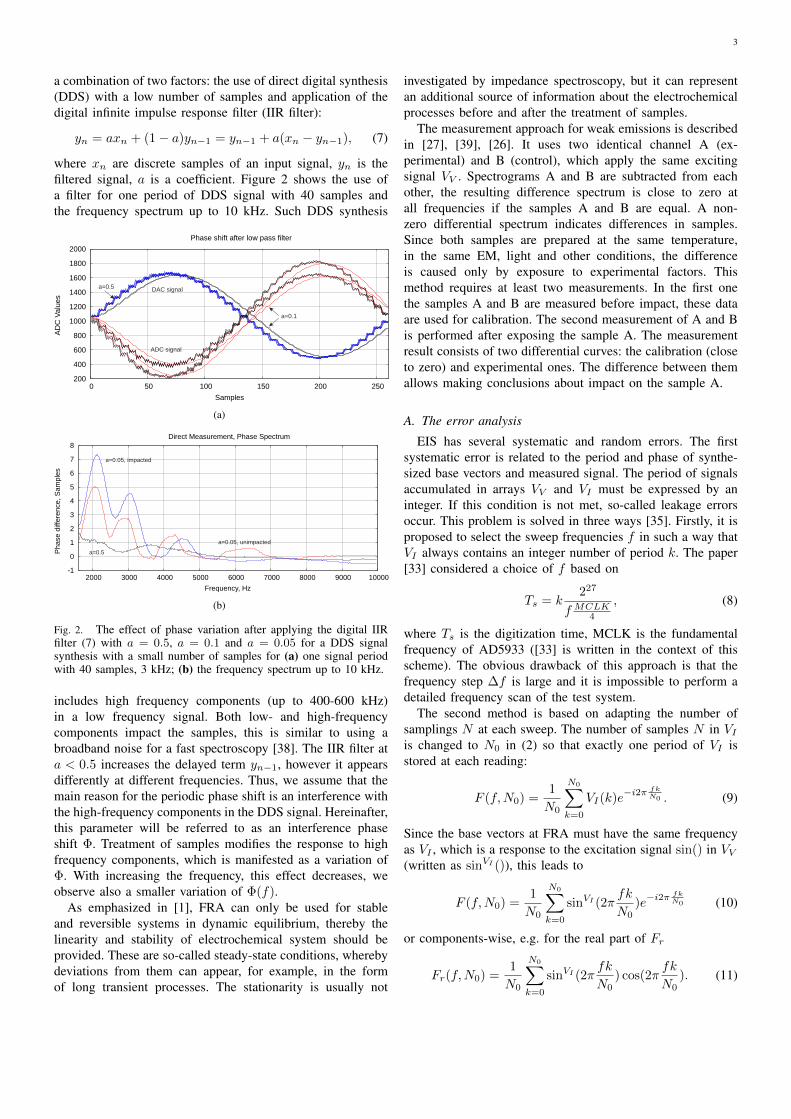
Despite f is disappeared from sin() and cos(), VI and VV arestill affected by the test system at frequencies f . Therefore,the physical meaning of (12) consists in analysis of amplitudevariation, phase and waveform of VI at the frequency f .The disadvantage of this method lies in the rapid decreaseof N0 when increasing the frequency f . Figure 3 shows therelationship between f and the number of samples N0 byselecting a different number of periods in the VI array. Thus,it is necessary to introduce the measurement ranges with adifferent number of periods.

0

200

400

600

800

1000

1200

1400

0

1x

5x

10x

20x

30x

40x

10 20 30 40 50 60 70 80 90 100

N o

f sa

mple

s

Frequency, kHz

N of samples vs. N of periods

1 period5 periods5 periods

20 periods30 periods40 periods

Fig. 3. The relationship between the frequency f and the number ofsamples N0 by selecting a different number of periods in VI .

The third approach consists in introducing so-called windowfunction W (N, k)

Fr(f) =1

N

N∑k=0

VI(k)W (N, k) cos(2πfk

N), (13)

which modulates the signal VI and reduces its amplitude toboundaries of window with N samples. The AD5933 uses theHanning function [35]:

W (N, k) =1

2

(1− cos(

2πk

N)

). (14)

The functions (13) allows keeping N at the same level for allfrequencies, which is useful for digitizing the signal. However,this method distorts the original signal, instead of VI(k) thesignal VI(k)W (N, k) is analyzed. This problem is discussedin literature [40]. Consequences of using (13) is reflected inFig. 9 as an appearance of new periodic components that arenot present in the original signal.

The second source of error is the frequency characteristics,and especially the limited bandwidth of analog components.As a result, the magnitude of VI decreases with f and themagnitude of the impedance Z ∼ 1

VIincreases. The problem

of increasing impedance exists in all EIS-meters, which solveit in different ways. For example, AD5933 requires two-pointor multi-point calibration [41] (see Section II-D).

The third source of systematic error represents a smallnumber of samples for DDS synthesis of VV when measuringthe test system with a large capacitive component. This leadsto peaks in VI and significantly increases noise, a detailedexamination of this effect for AD5933 is given in [33].

The impedance Z of test system and the reference resistanceRTIA in TIA should be similar

Z ∼ RTIA, (15)

otherwise the TIA can become saturated and the signal VI issignificantly distorted. Systematic errors are also influencedby the electrode polarization, which is a well-known prob-lem of impedance spectroscopy [42], [43], especially at lowfrequencies. This effect is markedly manifested when usingsmall-sized electrode and highly conductive liquids.

Random error also has several components. Firstly, a noiseintroduces a small random error of detecting the phase-amplitude characteristics of VV and VI . Secondly, the EISmeasurement interacts with samples due to the applied voltageand flowing current. When conducting multiple repeat mea-surements with the same sample, the measured parameters can’float’ – that introduces an additional error. A large randomerror occurs at variation of initial conditions for measurements.This includes small changes in the cell constant, temperaturevariations of containers and the liquid preparation. These smallvariations between control and experimental samples are wellmeasurable by the exact differential method and can lead towrong conclusions about the impacted fluid.

B. The EIS deviceMeasurement of weak emissions requires differential mea-

surement circuits and thermal stabilization of system andsamples. Available commercial EIS-meters do not offer theseoptions. In the previous works we used commercial conductiv-ity meters, the pH and Redox meters [26]. However they didnot provide accurate enough measurements, allowing to char-acterize weak emissions. In this work we decided to adapt theMU system [26], [27] for EIS measurements with necessarymethodology and metrology, and also to use available devicesfor control measurements. The first versions of MU-EIS onthe PSoC (Programmable System on Chip) architecture weredeveloped in 2012 [7], [44] and 2013 [39], [45] as devices forDC and non-contact high-frequency conductometry. The MU-EIS meter, see Fig. 4, supports differential measurements andtemperature control, the digital signal processing (DSP core) isimplemented in hardware on reconfigurable PSoC architecture.

The scheme AD5933 [41] has been selected as a commer-cially available solution. It is a precision impedance spectrom-eter on a single chip, which has an internal DSP core and isconnected to the host system by I2C interface. There are alarge number of available devices based on this scheme [33],[46], [47]. The termostabilization was performed by the MUsystem, two identical AD5933 boards are used for differentialEIS-meter, see Fig. 5. Software provided by Analog Deviceswas rewritten in order to support differential functions.

In general, both EIS-meters are similar. Synthesis of thesignal VV occurs by DDS (AD5933 – 27-bit frequency resolu-tion, MU-EIS – 32 bits), the I−V conversion is performed by

5

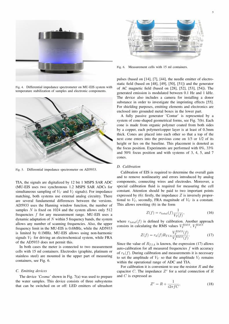
Fig. 4. Differential impedance spectrometer on MU-EIS system withtemperature stabilization of samples and electronic components.

Fig. 5. Differential impedance spectrometer on AD5933.

TIA, the signals are digitalized by 12 bit 1 MSPS SAR ADC(MU-EIS uses two synchronous 1.2 MSPS SAR ADCs forsimultaneous sampling of VV and VI signals). For impedancematching, both systems use external analog circuitry. Thereare several fundamental differences between the versions.AD5933 uses the Hanning window function, the number ofsamples N is fixed on 1024 and the system allows only 512frequencies f for any measurement range. MU-EIS uses adynamic adaptation of N within 5 frequency bands, the systemallows any number of scanning frequencies. Also, the upperfrequency limit in the MU-EIS is 0.6MHz, while the AD5933is limited by 0.1MHz. MU-EIS allows using non-harmonicsignals VV for driving an electrochemical system, while FRAof the AD5933 does not permit this.

In both cases the meter is connected to two measurementcells with 15 ml containers. Electrodes (graphite, platinum orstainless steel) are mounted in the upper part of measuringcontainers, see Fig. 6.

C. Emitting devices

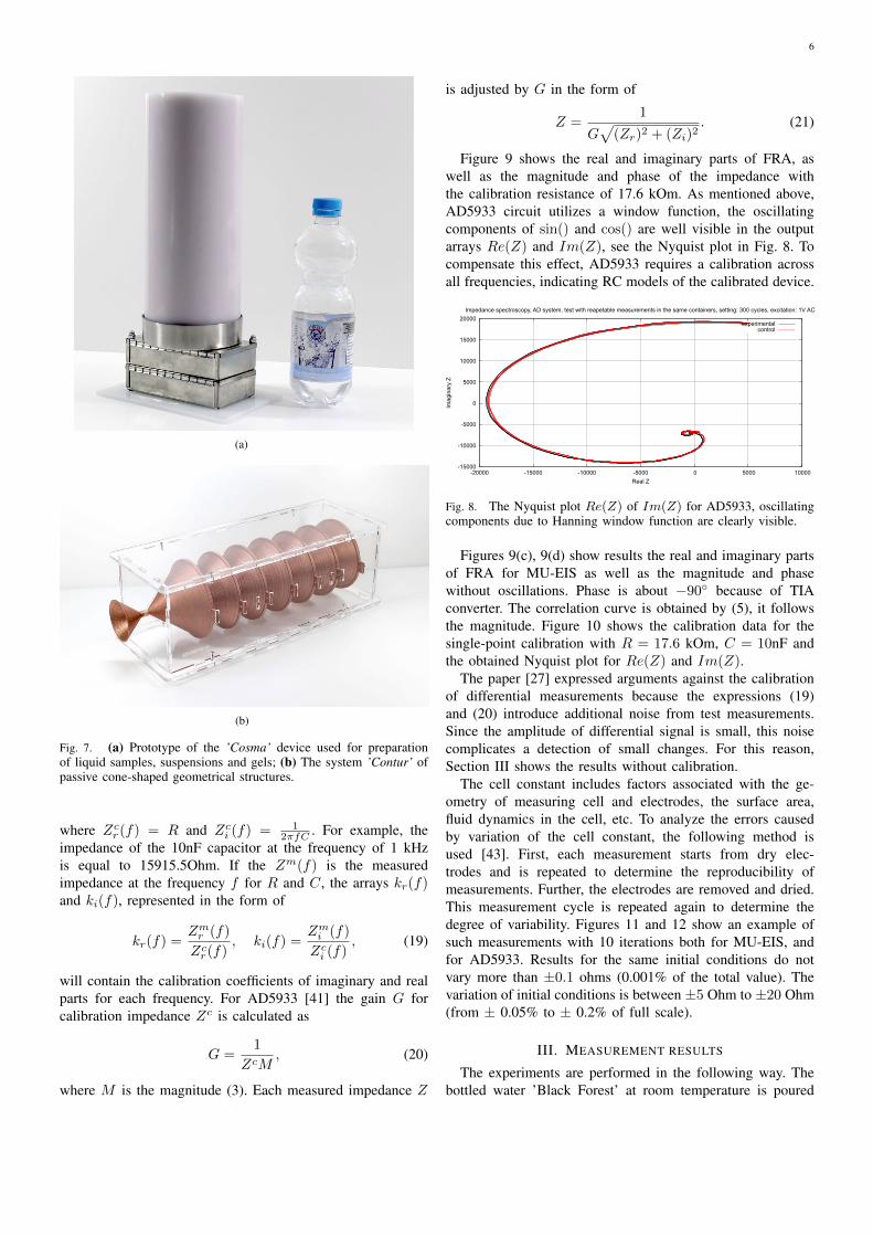
The device ’Cosma’ shown in Fig. 7(a) was used to preparethe water samples. This device consists of three subsystemsthat can be switched on or off: LED emitters of ultrashort

Fig. 6. Measurement cells with 15 ml containers.

pulses (based on [14], [7], [44], the needle emitter of electro-static field (based on [48], [49], [50], [51]) and the generatorof AC magnetic field (based on [28], [52], [53], [54]). Thegenerated emission is modulated between 0.1 Hz and 1 kHz.The device also includes a camera for installing a donorsubstance in order to investigate the imprinting effects [55].For shielding purposes, emitting elements and electronics areenclosed into grounded metal boxes in the lower part.

A fully passive generator ’Contur’ is represented by asystem of cone-shaped geometrical forms, see Fig. 7(b). Eachcone is made from organic polymer coated from both sidesby a copper, each polymer/copper layer is at least of 0.3mmthick. Cones are placed into each other so that a top of thenext cone enters into the previous cone on 1/3 or 1/2 of itsheight or lies on the baseline. This placement is denoted asthe focus position. Experiments are performed with 0%, 33%and 50% focus position and with systems of 3, 4, 5, and 7cones.

D. Calibration

Calibration of EIS is required to determine the overall gainand to remove nonlinearity and errors introduced by analogcomponents, connecting wires and electrodes. Moreover, aspecial calibration fluid is required for measuring the cellconstant. Attention should be paid to two important pointsexpressed by (6): firstly, the impedance Z is inversely propor-tional to VI , secondly, FRA magnitude of VV is a constant.This allows rewriting (6) in the form

Z(f) = rtotal(f)1

VI(f), (16)

where rtotal(f) is defined by calibration. Another approachconsists in calculating the RMS values V RMS

V , V RMSI

Z(f) = rk(f)RTIAV RMSV (f)

V RMSI (f)

. (17)

Since the value of RTIA is known, the expression (17) allowsauto-calibration for all measured frequencies f with accuracyof rk(f). During calibration and measurements it is necessaryto set the amplitude of VV so that the amplitude VI remainswithin the operational range of ADC and TIA.

For calibration it is convenient to use the resistor R and thecapacitor C. The impedance Zc for a serial connection of Rand C is expressed as

Zc = R+1

i2πfC, (18)

6

(a)

(b)

Fig. 7. (a) Prototype of the ’Cosma’ device used for preparationof liquid samples, suspensions and gels; (b) The system ’Contur’ ofpassive cone-shaped geometrical structures.

where Zcr(f) = R and Zci (f) = 12πfC . For example, the

impedance of the 10nF capacitor at the frequency of 1 kHzis equal to 15915.5Ohm. If the Zm(f) is the measuredimpedance at the frequency f for R and C, the arrays kr(f)and ki(f), represented in the form of

kr(f) =Zmr (f)

Zcr(f), ki(f) =

Zmi (f)

Zci (f), (19)

will contain the calibration coefficients of imaginary and realparts for each frequency. For AD5933 [41] the gain G forcalibration impedance Zc is calculated as

G =1

ZcM, (20)

where M is the magnitude (3). Each measured impedance Z

is adjusted by G in the form of

Z =1

G√

(Zr)2 + (Zi)2. (21)

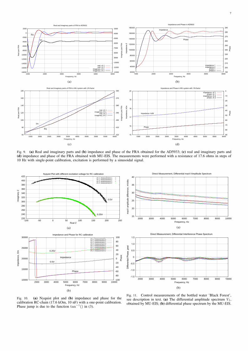
Figure 9 shows the real and imaginary parts of FRA, aswell as the magnitude and phase of the impedance withthe calibration resistance of 17.6 kOm. As mentioned above,AD5933 circuit utilizes a window function, the oscillatingcomponents of sin() and cos() are well visible in the outputarrays Re(Z) and Im(Z), see the Nyquist plot in Fig. 8. Tocompensate this effect, AD5933 requires a calibration acrossall frequencies, indicating RC models of the calibrated device.

-15000

-10000

-5000

0

5000

10000

15000

20000

-20000 -15000 -10000 -5000 0 5000 10000

Imagin

ary

Z

Real Z

Impedance spectroscopy, AD system, test with reapetable measurements in the same containers, setting: 300 cycles, excitation: 1V AC

controlexperimental

Fig. 8. The Nyquist plot Re(Z) of Im(Z) for AD5933, oscillatingcomponents due to Hanning window function are clearly visible.

Figures 9(c), 9(d) show results the real and imaginary partsof FRA for MU-EIS as well as the magnitude and phasewithout oscillations. Phase is about −90◦ because of TIAconverter. The correlation curve is obtained by (5), it followsthe magnitude. Figure 10 shows the calibration data for thesingle-point calibration with R = 17.6 kOm, C = 10nF andthe obtained Nyquist plot for Re(Z) and Im(Z).

The paper [27] expressed arguments against the calibrationof differential measurements because the expressions (19)and (20) introduce additional noise from test measurements.Since the amplitude of differential signal is small, this noisecomplicates a detection of small changes. For this reason,Section III shows the results without calibration.

The cell constant includes factors associated with the ge-ometry of measuring cell and electrodes, the surface area,fluid dynamics in the cell, etc. To analyze the errors causedby variation of the cell constant, the following method isused [43]. First, each measurement starts from dry elec-trodes and is repeated to determine the reproducibility ofmeasurements. Further, the electrodes are removed and dried.This measurement cycle is repeated again to determine thedegree of variability. Figures 11 and 12 show an example ofsuch measurements with 10 iterations both for MU-EIS, andfor AD5933. Results for the same initial conditions do notvary more than ±0.1 ohms (0.001% of the total value). Thevariation of initial conditions is between ±5 Ohm to ±20 Ohm(from ± 0.05% to ± 0.2% of full scale).

III. MEASUREMENT RESULTS

The experiments are performed in the following way. Thebottled water ’Black Forest’ at room temperature is poured

7

-18000

-16000

-14000

-12000

-10000

-8000

-6000

-4000

-2000

0

2000

1000 2000 3000 4000 5000 6000-12000

-11000

-10000

-9000

-8000

-7000

-6000

-5000

-4000

-3000

Real part

FR

A

Imagin

ary

part

FR

A

Frequency, Hz

Real and Imaginary parts of FRA in AD5933

real, ch 1real, ch 2

imaginary, ch 1imaginary, ch 2

Re

Im

(a)

Impedance and Phase in AD5933

Impedance

Z

Impedance

Phase

Phase

20000

40000

60000

80000

100000

120000

140000

160000

180000

1000 2000 3000 4000 5000 6000 190

200

210

220

230

240

250

260

270

280

290

Frequency, Hz

impedance 1impedance 2

phase 1phase 2

(b)

Real and Imaginary parts of FRA in MU system with 1/N factor

Re

Im

60

80

100

120

140

160

180

1500 2000 2500 3000 3500 4000 4500 5000 5500 6000-420

-410

-400

-390

-380

-370

-360

Real part

FR

A

Imagin

ara

part

FR

A

Frequency, Hz

real, ch 1imaginary, ch 1

real, ch 2imaginary, ch 2

(c)

Impedance and Phase in MU system with 1/N factor

Impedance =k/M

Phase

15

16

17

18

19

20

1500 2000 2500 3000 3500 4000 4500 5000 5500 6000-90

-80

-70

-60

-50

-40

-30

-20

-10

0

Imp

ed

an

ce,

kOm

Ph

ase

Frequency, Hz

impedance, ch 1phase, ch 1

impedance, ch 2phase, ch 2

(d)

Fig. 9. (a) Real and imaginary parts and (b) impedance and phase of the FRA obtained for the AD5933; (c) real and imaginary parts and(d) impedance and phase of the FRA obtained with MU-EIS. The measurements were performed with a resistance of 17.6 ohms in steps of10 Hz with single-point calibration, excitation is performed by a sinusoidal signal.

220

240

260

280

300

320

340

360

380

400

420

-100 -50

0.5V

0.25V

0 50 100 150 200 250

-Im

ag

ina

ry Z

Real Z

Nyquist Plot with different excitation voltage for RC calibration

ch 1: measurement 1ch 1: measurement 2ch 2: measurement 1ch 2: measurement 2

(a)

0.5V

0.25V

10000

15000

20000

25000

30000

2000 3000 4000 5000 6000 7000 8000 9000 10000-100

-80

-60

-40

-20

0

20

40

60

80

100

Imp

ed

an

ce,

Om

Ph

ase

Phase

Impedance

Frequency, Hz

Impedance and Phase for RC calibration

ch 1: measurement 1ch 1: measurement 2ch 2: measurement 1ch 2: measurement 2ch 1: measurement 1ch 1: measurement 2ch 2: measurement 1ch 2: measurement 2

(b)

Fig. 10. (a) Nyquist plot and (b) impedance and phase for thecalibration RC-chain (17.6 kOm, 10 nF) with a one-point calibration.Phase jump is due to the function tan−1() in (3).

15

20

25

30

35

40

2000 3000 4000 5000 6000 7000 8000 9000 10000

ma

xV a

mp

litu

de

diff

ere

nce

, m

Vo

lts

Frequency, Hz

Direct Measurement, Differential maxV Amplitude Spectrum

(a)

-1.5

-1.0

-0.5

0

0.5

1.0

1.5

2000 3000 4000 5000 6000 7000 8000 9000 10000

Diff

ere

ntia

l P

ha

se,

gra

d

Frequency, Hz

Direct Measurement, Differential Interference Phase Spectrum

(b)

Fig. 11. Control measurements of the bottled water ’Black Forest’,see description in text. (a) The differential amplitude spectrum VI ,obtained by MU-EIS; (b) differential phase spectrum by the MU-EIS.

8

-300

-200

-100

0

100

200

300

400

1000 2000 3000 4000 5000 6000 7000 8000 9000 10000

Diff

ere

ntial I

mpedance, O

m

Frequency, Hz

Impedance spectroscopy, AD system, test with reapetable measurements in the same containers, setting: 300 cycles, excitation: 1V AC

measurement 1measurement 2measurement 3measurement 4measurement 5measurement 6

Fig. 12. Control measurements of the bottled water ’Black Forest’with AD5933, differential impedance spectrum, see description intext.

into four 15 ml containers (two samples A and B) for AD5933and MU-EIS system. Samples thermostat is set on 27◦C. Thecontainers are kept in thermostat for 20 minutes to equalizethe temperature before starting measurements.

1. First test measurements are performed with A and Bsamples at frequencies between 1 kHz and 10 kHz with 10Hz steps. Sweeps are repeated 10 times, the spectra of A andB are subtracted from each other, as a result 10 differentialspectral curves are obtained. The purpose of this test is toassess the bias error of repeating measurements.

2. To determine the random error, the samples are removedfrom the thermostat and put on a shelf. After 30 minutes thesamples are placed again in the thermostat and 10 differentialmeasurements as described in (1) are performed.

3. The samples A and B are removed from the thermostat,the sample A is treated by ’Cosma’ or ’Contur’ devices.After this, the sample A is rested about 10 minutes, thenmeasurements with both samples are performed again.

4. To determine the random error after exposure, the samples(after exposure of the sample A) are removed from thethermostat, rested for 30 minutes, and then 10 differentialmeasurements are carried out.

Thus, this approach allows evaluating the variations ofsystematic and random errors as well as to estimate the effectof exposing the water to experimental factors. In total, 5 seriesof experiments with multiple iterations are performed.

Experimental Series 1. Figure 11 shows the results of oneof the control experiments with the procedure (1). The ampli-tude and phase characteristics show small changes caused byvariation of initial conditions. These experiments are repeatedmore than 20 times.

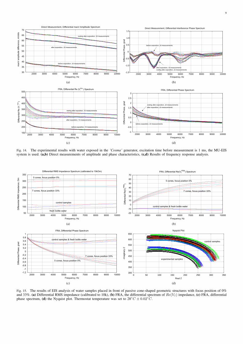
Experimental Series 2. This series has several dozen ofiterations, where various parameters of the module ’Cosma’are tested. The results of one of these experiments is shownin Fig. 14, where the procedures (2) and (3) are applied –water samples are exposed and the random error is estimatedafter the exposure. The exposition time varies between 10 and30 minutes. The variation of random error before and after theexposure has a similar character. However, significant changesare observed in the exposed samples. The measurement resultscan be characterized by ∆V diffI – amplitude changes of thedifferential signal (Re(V FRAI ), Re(Z), M(f), Corr(f) ex-hibit similar changes), ∆Φ - change of the interference phase

shift and ∆V stationaryI – variation of stationary conditions.Repeated measurements of the irradiated samples after 6-24hours show a strong variation at low frequencies that canindicate a change of electrochemical stability.

Experimental Series 3. These experiments are conductedwith the cone-shaped geometric structures. Containers withwater are placed in front of the output cone for 36 hours,see Fig. 13. Control measurements are performed with freshbottle water as well as with control containers rested for 36hours without any impact. Results of several measurementsare shown in Fig. 15. There are almost no differences betweencontrol samples and fresh bottle water, however, an essentialdifference between experimental and control samples. Sinceall containers are positioned in one room with the sameEM and other environmental factors, we can assume a non-electromagnetic impacting factor related to the shape effect.

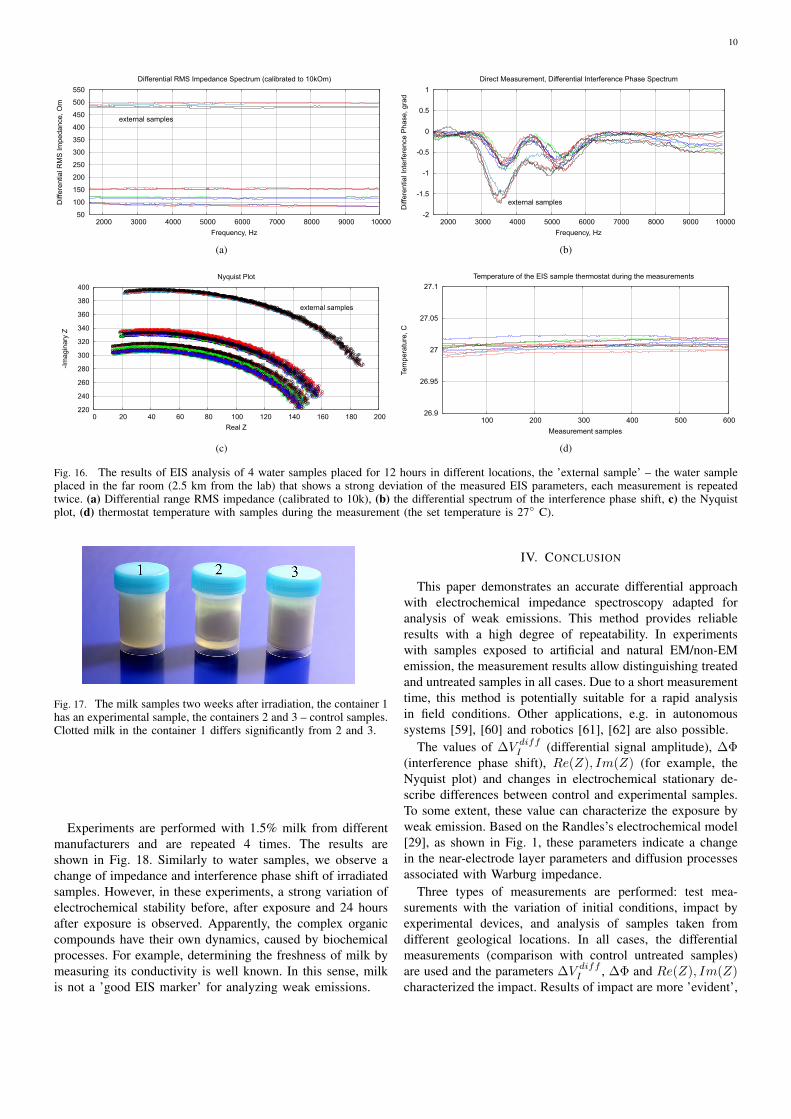
Experimental Series 4. For this series, four identicalsamples of water in 15 ml containers are placed for 12 hoursin different locations with the distance between 3 meters up to2.5 km from each other. This experiment is repeated 4 times.Fig. 16 shows the EIS results for one of the experiments. Inaddition, it shows the temperature of samples during measure-ments, the temperature fluctuations do not exceed 0.02◦C. The’external sample’ (sample from the far location) demonstratesthe largest changes of EIS parameters. Since the measuredvalues of EM and radiation background in these locationsare on the same level and conform to the EC/DIN norms,we can explain the EIS differences of samples only by somegeological or geo-biological factor.

Experimental Series 5. This series of experiments is moti-vated by the works of V.A.Sokolova’s group [20], where a gel-like consistency of milk exposed by the A.Deev’ generator wasachieved. Moreover, the well-known patents of R.Pavlita [56],A.Deev’s work [57] and ISTC VENT (group of A.E.Akimov)[58] indicated a capability of cleaning suspended solutionsexposed to some sources of weak emissions. For example,Fig. 17 shows samples of milk two weeks after irradiation inthe module ’Cosma’, we indeed observe a difference betweenexperimental and control samples of the clotted milk.

Fig. 13. Setup with cone-shaped geometric structures and watersamples.

9

2000

before exposition, 10 measurements

after exposition, 10 measurements

resting after exposition, 10 measurements

3000 4000 5000 6000 7000 8000 9000 10000

Frequency, Hz

30

35

40

45

50

55

60

65

70

ma

xV

am

plit

ud

e d

iffe

ren

ce,

mV

olts

Direct Measurement, Differential maxV Amplitude Spectrum

(a)




-1.5

-1.0

-0.5

0

0.5

1.0

1.5

2000 3000 4000 5000 6000 7000 8000 9000 10000

Diff

ere

ntia

l Ph

ase

, g

rad

Frequency, Hz


(b)




150

200

250

300

350

400

450

500

2000 3000 4000 5000 6000 7000 8000 9000 10000

Frequency, Hz

FRA, Differential Re (V

Diff

ere

ntia

l Re

(V

I

I

FRA

FR

A

) Spectrum

)

(c)




-1

-0.5

0

0.5

1

1.5

2

2.5

3

2000 3000 4000 5000 6000 7000 8000 9000 10000

Diff

ere

ntia

l Phase

, gra

d

Frequency, Hz

FRA, Differential Phase Spectrum

(d)

Fig. 14. The experimental results with water exposed in the ’Cosma’ generator, excitation time before measurement is 1 ms, the MU-EISsystem is used. (a,b) Direct measurements of amplitude and phase characteristics, (c,d) Results of frequency response analysis.

control samples

7 cones, focus position 33%


fresh bottle water 50

100

150

200

250

300

350

2000 3000 4000 5000 6000 7000 8000 9000 10000

Diff

ere

ntia

l RM

S Im

pedance, O

m

Frequency, Hz

Differential RMS Impedance Spectrum (calibrated to 10kOm)

(a)



control samples & fresh bottle water

-20

-10

0

10

20

30

40

50

60

70

2000 3000 4000 5000 6000 7000 8000 9000 10000

Diff

ere

ntia

l Re

(VIF

RA)

Frequency, Hz

FRA, Differential Re(VIFRA

) Spectrum

(b)



control samples & fresh bottle water

-1.2

-1

-0.8

-0.6

-0.4

-0.2

0

0.2

0.4

0.6

0.8

1

2000 3000 4000 5000 6000 7000 8000 9000 10000

Diff

ere

ntia

l P

ha

se

, g

rad

Frequency, Hz

FRA, Differential Phase Spectrum

(c)

control samples

experimental samples

300

350

400

450

500

550

600

650

0 50 100 150 200 250 300 350

-Im

ag

ina

ry Z

Real Z

Nyquist Plot

(d)

Fig. 15. The results of EIS analysis of water samples placed in front of passive cone-shaped geometric structures with focus position of 0%and 33%. (a) Differential RMS impedance (calibrated to 10k), (b) FRA, the differential spectrum of Re(VI) impedance, (c) FRA, differentialphase spectrum, (d) the Nyquist plot. Thermostat temperature was set to 28◦C ± 0.02◦C.

10

50

100

150

200

250

300

350

400

450

500

550

2000 3000 4000 5000

external samples

6000 7000 8000 9000 10000

Diff

ere

ntia

l R

MS

Im

pedance, O

m

Frequency, Hz


(a)

external samples

-2

-1.5

-1

-0.5

0

0.5

1

2000 3000 4000 5000 6000 7000 8000 9000 10000

Diff

ere

ntia

l In

terf

ere

nce

Ph

ase

, g

rad

Frequency, Hz


(b)

external samples

220

240

260

280

300

320

340

360

380

400

0 20 40 60 80 100 120 140 160 180 200

-Im

agin

ary

Z

Real Z

Nyquist Plot

(c)

26.9

26.95

27

27.05

27.1

100 200 300 400 500 600

Tem

pe

ratu

re,

C

Measurement samples

Temperature of the EIS sample thermostat during the measurements

(d)

Fig. 16. The results of EIS analysis of 4 water samples placed for 12 hours in different locations, the ’external sample’ – the water sampleplaced in the far room (2.5 km from the lab) that shows a strong deviation of the measured EIS parameters, each measurement is repeatedtwice. (a) Differential range RMS impedance (calibrated to 10k), (b) the differential spectrum of the interference phase shift, c) the Nyquistplot, (d) thermostat temperature with samples during the measurement (the set temperature is 27◦ C).

Fig. 17. The milk samples two weeks after irradiation, the container 1has an experimental sample, the containers 2 and 3 – control samples.Clotted milk in the container 1 differs significantly from 2 and 3.

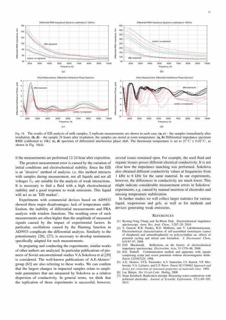
Experiments are performed with 1.5% milk from differentmanufacturers and are repeated 4 times. The results areshown in Fig. 18. Similarly to water samples, we observe achange of impedance and interference phase shift of irradiatedsamples. However, in these experiments, a strong variation ofelectrochemical stability before, after exposure and 24 hoursafter exposure is observed. Apparently, the complex organiccompounds have their own dynamics, caused by biochemicalprocesses. For example, determining the freshness of milk bymeasuring its conductivity is well known. In this sense, milkis not a ’good EIS marker’ for analyzing weak emissions.

IV. CONCLUSION

This paper demonstrates an accurate differential approachwith electrochemical impedance spectroscopy adapted foranalysis of weak emissions. This method provides reliableresults with a high degree of repeatability. In experimentswith samples exposed to artificial and natural EM/non-EMemission, the measurement results allow distinguishing treatedand untreated samples in all cases. Due to a short measurementtime, this method is potentially suitable for a rapid analysisin field conditions. Other applications, e.g. in autonomoussystems [59], [60] and robotics [61], [62] are also possible.

The values of ∆V diffI (differential signal amplitude), ∆Φ(interference phase shift), Re(Z), Im(Z) (for example, theNyquist plot) and changes in electrochemical stationary de-scribe differences between control and experimental samples.To some extent, these value can characterize the exposure byweak emission. Based on the Randles’s electrochemical model[29], as shown in Fig. 1, these parameters indicate a changein the near-electrode layer parameters and diffusion processesassociated with Warburg impedance.

Three types of measurements are performed: test mea-surements with the variation of initial conditions, impact byexperimental devices, and analysis of samples taken fromdifferent geological locations. In all cases, the differentialmeasurements (comparison with control untreated samples)are used and the parameters ∆V diffI , ∆Φ and Re(Z), Im(Z)characterized the impact. Results of impact are more ’evident’,

11

control, no exposure

after exposure

40

60

80

100

120

140

160

2000 3000 4000 5000 6000 7000 8000 9000 10000

Diff

ere

ntia

l RM

S I

mp

ed

an

ce,

Om

Frequency, Hz


(a)

50

100

150

200

250

300

350

400

450

2000 3000 4000


after exposure

5000 6000 7000 8000 9000 10000

Diff

ere

ntia

l RM

S I

mp

ed

an

ce,

Om

Frequency, Hz


(b)


after exposure

-1

0

1

2

3

4

5

6

2000 3000 4000 5000 6000 7000 8000 9000 10000

Diff

ere

ntia

l In

terf

ere

nce

Ph

ase

, g

rad

Frequency, Hz


(c)


after exposure

-10

-8

-6

-4

-2

0

2

2000 3000 4000 5000 6000 7000 8000 9000 10000

Diff

ere

ntia

l In

terf

ere

nce

Ph

ase

, g

rad

Frequency, Hz


(d)

Fig. 18. The results of EIS analysis of milk samples, 5 replicate measurements are shown in each case, (a, c) – the samples immediately afterirradiation, (b, d) – the sample 24 hours after irradiation, the samples are stored at room temperature. (a, b) Differential impedance spectrumRMS (calibrated to 10k); (c, d) spectrum of differential interference phase shift. The thermostat temperature is set to 27◦C ± 0.02◦C, asshown in Fig. 16(d).

if the measurements are performed 12-24 hour after exposition.The greatest measurement error is caused by the variation of

initial conditions and electrochemical stability. Since the EISis an ’invasive’ method of analysis, i.e. this method interactswith samples during measurement, not all liquids and not allvoltages VV are suitable for the analysis of weak interactions.It is necessary to find a fluid with a high electrochemicalstability and a good response to weak emissions. This liquidwill act as an ’EIS marker’.

Experiments with commercial devices based on AD5933showed three major disadvantages: lack of temperature stabi-lization, the inability of differential measurements and FRAanalysis with window functions. The resulting error of suchmeasurements are often higher than the amplitude of measuredsignals caused by the impact of experimental factors. Inparticular, oscillations caused by the Hanning function inAD5933 complicate the differential analysis. Similarly to thepotentiometry [26], [27], is necessary to develop instrumentsspecifically adapted for such measurements.

In preparing and conducting the experiments, similar worksof other authors are analyzed. In particular publications of pio-neers of Soviet unconventional studies V.A.Sokolova et al [20]is considered. The well-known publications of A.E.Akimov’group [63] are also referring to these works. We can confirmthat the largest changes in impacted samples relate to ampli-tude parameters that are measured by Sokolova as a relativedispersion of conductivity. In general terms, we think thatthe replication of those experiments is successful, however,

several issues remained open. For example, the used fluid andorganic tissues posses different electrical conductivity. It is notclear how the impedance matching was performed. Sokolovaalso obtained different conductivity values at frequencies from1 kHz to 8 kHz for the same material. In our experiments,however, the differences in conductivity are much lower. Thismight indicate considerable measurement errors in Sokolova’experiments, e.g. caused by manual insertion of electrodes andmissing temperature stabilization.

In further studies we will collect larger statistics for variousliquid, suspensions and gels, as well as for methods anddevices generating weak emissions.

REFERENCES

[1] Byoung-Yong Chang and Su-Moon Park. Electrochemical impedancespectroscopy. Annu. Rev. Anal. Chem., 3:207–29, 2010.

[2] V. Ganesh, R.R. Pandey, B.D. Malhotra, and V. Lakshminarayanan.Electrochemical characterization of self-assembled monolayers (sams)of thiophenol and aminothiophenols on polycrystalline au: effects ofpotential cycling and mixed sam formation. J. Electroanal. Chem,619:87–97, 2008.

[3] D.D. Macdonald. Reflections on the history of electrochemicalimpedance spectroscopy. Electrochim. Acta, 51:1376–88, 2006.

[4] H.E. Puthoff. Communication method and apparatus with signalscomprising scalar and vector potentials without electromagnetic fields.Patent US5845220, 1998.

[5] A.E. Akimov, V.Ch. Tarasenko, A.V. Samochin, I.V. Kurick, V.P. Mei-boroda, V.A. Licharev, and U.F. Perov. Patent SU1748662 Approach anddevice for correction of structural properties of materials (rus). 1992.

[6] Luc Burgin. Der Urzeit-Code. Herbig, 2008.[7] Serge Kernbach. Replication attempt: Measuring water conductivity with

polarized electrodes. Journal of Scientific Exploration, 27(1):69–105,2013.

12

[8] I.R.Kumar, N.V.C.Swamy, and H.R.Nagendra. Effect of pyramids onmicroorganisms. Indian Journal of Traditional Knowledge, 4(4):373–379, 2005.

[9] S.V. Mjkin, I.V. Vasilieva, and A.V. Rudenko. Investigation of theinfluence of the field generated by a pyramid on the material objects(rus). Consciousness and physical reality, (7(2)):45–53, 2002.

[10] Brenda J. Dunne and Robert G. Jahn. Consciousness and anomalousphysical phenomena. Technical Note PEAR 95004, 1995.

[11] H. Schmidt. Mental influence on random events. New Scientist andScience Journal, pages 757–758, 1971.

[12] Peter Tompkins and Christopher Bird. The Secret Life of Plants.Hardcover, 1973.

[13] V. Bobrov. Reaction of double electrical layer on torsion field (rus). InBINITI N 1055-B97, 1997.

[14] A.V. Bobrov. Investigating a field concept of consciousness (rus). Orel,Orel University Publishing, 2006.

[15] C. Cardella, L. de Magistris, E. Florio, and C.W. Smith. Permanentchanges in the physico-chemical properties of water following exposureto resonant circuits. Journal of Scientific Exploration, (15(4)):501–518,2001.

[16] H. Stenschke. Polarization of water in the metal/electrolyte interface.Journal of Electroanalytical Chemistry and Interfacial Electrochemistry,196(2):261 – 274, 1985.

[17] David W. R. Gruen and Stjepan Marcelja. Spatially varying polarizationin water. a model for the electric double layer and the hydration force.J. Chem. Soc., Faraday Trans. 2, 79:225–242, 1983.

[18] M. L. Belaya, M. V. Feigel’man, and V. G. Levadnyii. Structural forcesas a result of nonlocal water polarizability. Langmuir, 3(5):648–654,1987.

[19] J. Lyklema. Fundamentals of Interface and Colloid Science. AcademicPress, 2005.

[20] V.A.Sokolova. First experimental confirmation of torsion fields and theirusage in agriculture (rus). Moscow, 2002.

[21] M.A. Andriasheva. Changing water properties through numeric codes(rus). IJUS, 10(3):7–14, 2015.

[22] V.G.Krasnobrygev and M.V.Kurick. Properties of coherent water (rus).Quantum Magic, 7(2):2161–2166, 2010.

[23] Mark Krinker. Spinning process based info-sensors. Proc. of the 3rdint. conf. ’Torsion fields and information interactions’, pages 223–228,2012.

[24] M. Krinker, A. Goykadosh, and H. Einhorn. On the possibility oftransferring information with non-electromagnetic fields, the relation ofspinning processes and encoding information and the hydrogen spindetector. In Systems, Applications and Technology Conference (LISAT),2012 IEEE Long Island, pages 1–12, May 2012.

[25] S. Kernbach. The minimal experiment (rus). International Journal ofUncoventional Science, 4(2):50–61, 2014.

[26] S.Kernbach and O.Kernbach. On precise pH and dpH measurements(rus). International Journal of Unconventional Science, 5(2):83–103,2014.

[27] S. Kernbach and O. Kernbach. Detection of ultraweak interactions byprecision dph approach (rus). IJUS, 9(3):17–41, 2015.

[28] V.N. Anosov and E.M. Truchan. New approach to impact of weakmagnetic fields on living objects (rus). Doklady Akedemii Nauk:biochemistry, biophysics and molecular biology, (392):1–5, 2003.

[29] J.E.B. Randles. Kinetics of rapid electrode reactions. Discuss. FaradaySoc., 1:11–19, 1947.

[30] U.V. Tkachuk, S.D.Jremchuk, and A.A.Fedotov. Experimental studyof the effect of rotating ferrite magnetic disks on the reaction ofacetic anhydride hydration (rus). The II int. conf. ’Torsion fields andinformation interactions’, pages 106–110, 2010.

[31] Agilent Technologies. Agilent Impedance Measurement Handbook.Agilent, 2013.

[32] P.Norouzi, M.Pirali-Hamedani, T.M.Garakani, and M.R.Ganjali. Ap-plication of fast fourier transforms in some advanced electroanalyticalmethods. in: Fourier Transforms – New Analytical Approaches and FTIRStrategies, (ed.) G.Nikolic, pages 303–322, 2011.

[33] K. Chabowski, T.Piasecki, A.Dzierka, and K. Nitsch. Simple widefrequency range impedance meter based on AD5933 integrated circuit.Metrology and Measurement Systems, XXII(1):13–24, 2015.

[34] Jong-Wook Kim, ByungKoo Park, Seung Cheol Jeong, Sang WooKim, and PooGyeon Park. Fault diagnosis of a power transformerusing an improved frequency-response analysis. Power Delivery, IEEETransactions on, 20(1):169–178, Jan 2005.

[35] L.Matsiev. Improving performance and versatility of systems based onsingle-frequency dft detectors such as ad5933. Electronics, 4(1):1–34,2015.

[36] J. Ojarand and M. Min. Simple and efficient excitation signals for fastimpedance spectroscopy. Elektronika ir Elektrotechnika, 19(2):1392–1215, 2013.

[37] A.Meja-Aguilar and R.Palls-Areny. Electrical impedance measurementusing voltage/current pulse excitation. XIX IMEKO World Congress,Fundamental and Applied Metrology, pages 662–667, 2009.

[38] D.E. Smith. The acquisition of electrochemical response spectra by on-line fast fourier transform. Data processing in electrochemistry. Anal.Chem., 48:A221–40, 1976.

[39] S. Kernbach. On metrology of systems operating with ’high-penetrating’emission (rus). International Journal of Unconventional Science,1(2):76–91, 2013.

[40] F.J. Harris. On the use of windows for harmonic analysis with thediscrete fourier transform. IEEE Proc., 66:5183, 1978.

[41] Analog Devices. Data sheet AD5933: 1 MSPS, 12-Bit ImpedanceConverter, Network Analyzer. Analog Devices, 2005-2013.

[42] Paul Ben Ishai, Mark S Talary, Andreas Caduff, Evgeniya Levy, and YuriFeldman. Electrode polarization in dielectric measurements: a review.Measurement Science and Technology, 24(10):102001, 2013.

[43] Kalvoy H, Johnsen GK, Martinsen OG, and Grimnes S. New methodfor separation of electrode polarization impedance from measured tissueimpedance. The Open Biomedical Engineering Journal, 5:8–13, 2011.

[44] S. Kernbach. Exploration of high-penetrating capability of LED andlaser emission. Parts 1 and 2 (rus). Nano- and microsystem’s technics,6,7:38–46,28–38, 2013.

[45] Serge Kernbach and Olga Kernbach. Impact of structural elements onhigh frequency non-contact conductometry. in publication, 2013.

[46] S.A. Ghaffari, W.-O. Caron, M. Loubier, M. Rioux, J. Viens, B. Gosselin,and Y. Messaddeq. A wireless multi-sensor dielectric impedancespectroscopy platform. Sensors, 15:23572–23588, 2015.

[47] Jerzy Hoja and Grzegorz Lentka. Interface circuit for impedance sensorsusing two specialized single-chip microsystems. Sensors and ActuatorsA: Physical, 163(1):191 – 197, 2010.

[48] A.I.Weinik. Book of sorrow (rus). Minsk manuscript, 1981.[49] A.I.Weinik. Thermodynamics of real processes (rus). Minks: ’Nauka i

technika’, 1991.[50] A.L.Chigewskij. Electric and magnetic properties of erythrocytes (rus).

Moscow, 1973.[51] A.L.Chigewskij. Epidemiological catastrophes and periodic activity of

the Sun. Moscow, 1930.[52] G.Dulnev. Looking for a new world (rus). Wes, 2004.[53] A.A. Asheulow, U.B. Dobrovolskij, and V.A. Besulik. Impact of electric

and magnetic fields on parameters of semiconductor devices. Technologyand design in electronic equipment, (1):33–35, 2000.

[54] A.A.Britova, I.V.Adamko, and V.L.Bachurina. Activation of water bylaser light, magnetic field or by their combination (rus). Vesnik ofNovgorod’s State University, (7), 1998.

[55] S. Kernbach. Supernatural. Scientifically proven facts. Algorithm.Moscow, 2015.

[56] The Pavlita Foundation. Note on work of Robert Pavlita and his exper-iments in bio-energy. www.keelynet.com/biology/pavlita1.txt, 1992.

[57] Edwin C. May, Victor Rubel, and Loyd Auerbach. ESP WARS: East andWest: An Account of the Military Use of Psychic Espionage As Narratedby the Key Russian and American Players. CreateSpace IndependentPublishing Platform, 2014.

[58] S. Kernbach. Unconventional research in USSR and Russia: shortoverview. arXiv 1312.1148, 2013.

[59] P. Levi, M. Schanz, S. Kornienko, and O. Kornienko. Application of or-der parameter equation for the analysis and the control of nonlinear timediscrete dynamical systems. Int. J. Bifurcation and Chaos, 9(8):1619–1634, 1999.

[60] A. E. Eiben, N. Ferreira, M. C. Schut, and S. Kernbach. Embodiedartificial evolution: the future of artificial evolutionary systems. In Proc.of the 13th conf. on Genetic and evolutionary computation, GECCO ’11,pages 27–28, New York, NY, USA, 2011. ACM.

[61] S. Kornienko, O. Kornienko, and P. Levi. Swarm embodiment - a newway for deriving emergent behaviour in artificial swarms. In P.Levi andet al., editors, Autonome Mobile Systeme (AMS’05), pages 25–32, 2005.

[62] O. Kornienko, S. Kornienko, and P. Levi. Collective decision makingusing natural self-organization in distributed systems. In Proc. ofInt. Conf. on Computational Intelligence for Modelling, Control andAutomation (CIMCA’2001), Las Vegas, USA, pages 460–471, 2001.

[63] A.E. Akimov, V.J. Tarasenko, and S.U. Tolmachev. Torsion communica-tion – new system for telecommunication (rus). Electrocommunication,(5), 2001.

Documents

On accurate differential measurements with electrochemical ... · On accurate differential measurements with electrochemical impedance spectroscopy S.Kernbach, I.Kuksin, O.Kernbach