On a Spectral Theorem of Weyl

Nigel Higson and Qijun Tan

Abstract

We give a geometric proof of a theorem of Weyl on the continuouspart of the spectrum of Sturm-Liouville operators on the half-line withasymptotically constant coefficients. Earlier proofs due to Weyl andKodaira depend on special features of Green’s functions for linearordinary differential operators; ours might offer better prospects forgeneralization to higher dimensions, as required for example in non-commutative harmonic analysis.

1 Introduction

The purpose of this paper is to present a new approach to an old theoremof Hermann Weyl on the spectral theory of self-adjoint Sturm-Liouville op-erators on a half-line. Our aim is to invoke methods that are geometric inspirit, and more amenable to generalization, for instance to Plancherel for-mulas for spherical functions (this is an area that is closely related to Weylswork). We shall however stay fairly close to Weyl’s original context in thisarticle.

Sturm-Liouville theory is of course concerned with the eigenvalues andeigenfunctions of linear differential operators

(1.1) D = −d

dx· p(x) · d

dx+ q(x),

initially on a closed interval [a, b]. Assume for simplicity that p(x) and q(x)are smooth, real-valued functions on [a, b], with p(x) positive everywhere.In examining the solutions of the eigenvalue problem

(1.2) Dfλ = λfλ,

it is conventional to impose boundary conditions, and the most obviouschoice is

(1.3) fλ(a) = 0 = fλ(b).

1

arX

iv:1

611.

0339

6v2

[m

ath.

OA

] 4

Apr

201

7

The elements of Sturm-Liouville theory can then be summarized as fol-lows,1 using the L2-inner product 〈f, h〉:

1.1 Theorem. The eigenvalues λ for the above problem are real numbers, and eachhas multiplicity one. The set of all eigenvalues is a discrete subset of R, boundedbelow, and if h is any smooth function on [a, b], then

h(x) =∑λ

〈fλ, h〉〈fλ, fλ〉

fλ(x)

for x ∈ (a, b).

In an influential paper [Wey10] from early in his career, Weyl developedan analogous theory for Sturm-Liouville operators on [0,∞). Weyl’s paperaddressed many issues, but our concern here is his treatment of the contin-uous spectrum of a Sturm-Liouville operator, and especially his version forthe continuous spectrum of the expansion theorem above, which we shallnow describe.

Weyl assumes that the coefficient functions p(x) and q(x) in (1.1) con-verge sufficiently rapidly to the constants 1 and 0, respectively, as x tendsto infinity. For the purposes of this introduction, let us assume even more,namely that

(1.4) p(x) ≡ 1 and q(x) ≡ 0 if x� 0

(this assumption is too strong to be interesting in applications, but it al-lows us to quickly introduce Weyl’s ideas). For each λ ∈ C there is a one-dimensional space of eigenfunctions2 Fλ for D that satisfy the boundarycondition

(1.5) Fλ(0) = 0.

If we focus on the case where λ > 0, and if we choose, as we may, Fλ to benonzero and real-valued, then our assumptions on the coefficient functionsp(x) and q(x) imply that

(1.6) Fλ(x) = c(λ)ei√λ x + c(λ)e−i

√λ x if x� 0,

for some nonzero c(λ) ∈ C. We can now formulate Weyl’s result, at least inthe simplified context of (1.4) that we are currently discussing.

1For a precise formulation of the theorem and a thorough account of its proof, see forexample [DS88, Chapter XIII], especially Theorem 3 in Section 4.

2We write Fλ rather than fλ as a reminder that the eigenfunction need not be square-integrable in this context; in fact it is better to view it as a distribution.

2

1.2 Theorem. If h is a smooth, compactly supported function on [0,∞), then3

h(x) =∑λ<0

〈Fλ, h〉〈Fλ, Fλ〉

Fλ(x) +1

4π

∫∞0

〈Fλ, h〉|c(λ)|2

Fλ(x)dλ√λ

for x ∈ (0,∞). The first sum is over the square-integrable eigenfunctions asso-ciated to negative eigenvalues that satisfy the boundary condition (1.5), and thereare finitely many of these.

We shall approach Weyl’s theorem by comparing the Sturm-Liouvilleoperator D to the simpler operator

D0 = −d2

dx2

on (−∞,∞). Our argument is roughly as follows. General theory guaran-tees an integral decomposition

(1.7) h(x) =

∫〈Fλ, h〉 Fλ(x)dµ(λ)

for some measure on the spectrum of D. If h is supported sufficiently faraway from 0 ∈ [0,∞), then, in view of (1.6), the integral in (1.7) can beviewed as a sort of approximate decomposition of h over the spectrumof D0. It is not exact because (1.7) involves the negative spectrum of D,which has no counterpart for D0, and more crucially because it involvesonly some, but not all the eigenfunctions on D0 (there are two linearly in-dependent eigenfunctions ofD0 for every λ > 0, but only one specific linearcombination contributes to the integral). However we can put together theintegral formulas in (1.7) for all the forward translates of h along the lineby averaging, and then invoke the translation-invariance ofD0 to obtain anexact formula for the spectral decomposition of D0 in terms of the muea-sure µ. Finally, we can invert this formula to describe the (positive part ofthe) spectral theory of D in terms of the spectral theory of D0, which is ofcourse known, and from this we shall recover Weyl’s formula.

We shall give an abstract account of our approach in Section 3, wherethe main results are Theorems 3.3 and 3.6. Our reason for doing this isthat other interesting instances of the abstract framework arise in harmonic

3We won’t discuss in this introduction the nature of the convergence in the eigenfunctionexpansion, but see for example [Ban08] or [EK08], as well as the original source, of course,for more details. We shall make precise statements in the language of spectral theory laterin the paper.

3

analysis, as we shall note in Section 3 (however we shall postpone untila future paper a detailed treatment of these examples). We shall applyour method to the continuous spectrum of Sturm-Liouville operators inSection 4, and we shall address the discrete part of the spectrum of D inSection 5. But prior to all of that we shall quickly review the standardapproach in Section 2 for the sake of comparison.

This work grew in part out of a project in noncommutative geome-try [CCH16, CH16], which led us to try to understand more about thePlancherel formula, and hence Weyl’s theorem. Remarking on Weyl’s in-fluence on representation theory, Borel [Bor01, p.38] writes that

“It was the reading of [Weyl’s 1910 paper] which suggested toHarish-Chandra that the measure should be the inverse of thesquare modulus of a function in λ describing the asymptoticbehaviour of the eigenfunctions . . . and I remember well fromseminar lectures and conversations that he never lost sight ofthat principle, which is confirmed by his results in the generalcase.”

We believe that the approach to Weyl’s theorem presented here offers goodprospects for an alternative approach to some of Harish-Chandra’s results.

2 Review of Kodaira’s Approach

In this section we shall very briefly review the approach to Theorem 1.2developed by Weyl [Wey10] and then substantially improved by Kodaira[Kod49]; see also [Wey50]. For brevity we shall continue to consider onlythe simplest possible case of a Sturm-Liouville operatorD on [0,∞) whosecoefficients are eventually constant, as in (1.4).

We shall take it for granted that D defines an essentially self-adjointoperator on L2(0,∞), with initial domain the smooth, compactly supportedfunctions on [0,∞) that vanish at 0, as in (1.5). We shall concentrate hereon the positive part of the spectrum of D and hence the integral expressionin Theorem 1.2.

Of interest to us, therefore, are the spectral projections P[α,β] for D as-sociated to closed intervals [α,β] in the positive real numbers. FollowingKodaira we shall prove the following version of Weyl’s theorem:

2.1 Theorem. If β > α > 0, then spectral projection P[α,β] for D is given by the

4

formula

(P[α,β]h)(x) =

∫∞0

p[α,β](x, y)h(y)dy,

where

(2.1) p[α,β](x, y) =1

4π

∫βα

Fλ(x)Fλ(y)1

|c(λ)|2dλ√λ.

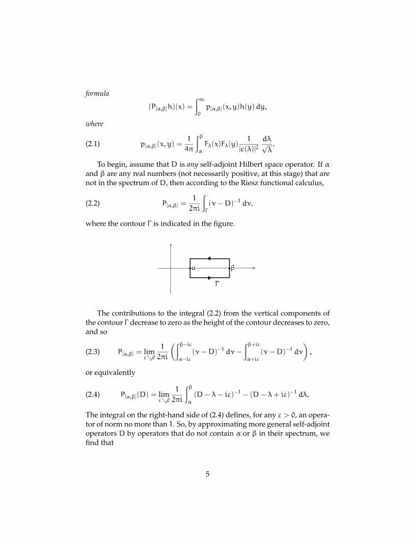
To begin, assume that D is any self-adjoint Hilbert space operator. If αand β are any real numbers (not necessarily positive, at this stage) that arenot in the spectrum of D, then according to the Riesz functional calculus,

(2.2) P[α,β] =1

2πi

∫Γ

(ν−D)−1 dν.

where the contour Γ is indicated in the figure.

The contributions to the integral (2.2) from the vertical components ofthe contour Γ decrease to zero as the height of the contour decreases to zero,and so

(2.3) P[α,β] = limε↘0 1

2πi

(∫β−iεα−iε

(ν−D)−1 dν−

∫β+iεα+iε

(ν−D)−1 dν

),

or equivalently

(2.4) P[α,β](D) = limε↘0 1

2πi

∫βα

(D− λ− iε)−1 − (D− λ+ iε)−1 dλ.

The integral on the right-hand side of (2.4) defines, for any ε > 0, an opera-tor of norm no more than 1. So, by approximating more general self-adjointoperators D by operators that do not contain α or β in their spectrum, wefind that

5

2.2 Lemma (Kodaira). The formula (2.4) holds for any self-adjoint operator Dand any interval [α,β], as long as as α and β do not belong to the point spectrumof D.

The value of the Kodaira formula4 is that when D is a Sturm-Liouvilleoperator, the resolvent operators, particularly in the combination they ap-pear in (2.4), may be computed quite explicitly. First of all, if ν ∈ C \ R,then we may write

(D− ν)−1h =

∫∞0

kν(x, y)h(y)dy

The kernel kν(x, y) has the following properties:

(a) kν is continuous on [0,∞)×[0,∞), smooth away from the diagonal, andconverges to zero as x→ ∞ or y→ ∞.

(b) kν(x, y) = 0when x = 0 or y = 0.

(c) kν(y, x) = kν(x, y).

(d) (D− ν)kν( , y) = δy

Now let Fν be a ν-eigenfunction for D that vanishes at 0, and let Gν bea ν-eigenfunction that vanishes at infinity. It follows rather easily from theabove list of properties that

kν(x, y) =1

w(ν)Fν(x)Gν(y) when x < y,

for some constant w(λ) 6= 0 (independent of x and y). Using (d) one com-putes that

(2.5) w(ν) = −wx(Fν, Gν) = −p(x)(Fν(x)G

′ν(x) − F

′ν(x)Gν(x)

)(this is independent of x). This is an application of the relation

(2.6)∫ba

(Dg)(y)h(y)dy−

∫ba

g(y)(Dh)(y)dy = wa(g, h) −wb(g, h)

where

(2.7) wx(g, h) = p(x)(g(x)h ′(x) − g ′(x)h(x)

).

4The same formula was obtained in a slightly different context by Titchmarsh [Tit46],and the term “Kodaira-Titchmarsh formula” is therefore often used.

6

To return to Kodaira’s formula, we find that the integrand in (2.4) isrepresented by the integral kernel

(2.8) w(λ+ iε)−1Fλ+iε(x)Gλ+iε(y) −w(λ− iε)−1Fλ−iε(x)Gλ−iε(y)

when x < y. At this point we finally use the fundamental assumption (1.4)on the coefficients of D. First, Gν(y) is a constant times ei

√νy where the

square root with positive imaginary part is chosen to ensure Gν vanishes atinfinity. Keeping this and (2.5) in mind, we compute the limit of (2.8) asε↘ 0 to be

−1

2i√λ|c(λ)|2

Fλ(x)Fλ(y).

It follows that

(2.9)P[α,β](D) =

1

2πi

∫βα

−1

2i√λ|c(λ)|2

Fλ(x)Fλ(y)dλ

=1

4π

∫βα

Fλ(x)Fλ(y)1

|c(λ)|2dλ√λ,

as required.

3 Asymptotically Related Representations

In this section we shall describe our alternative method of computing thecontinuous part of the spectral measure in Weyl’s theorem. Like Kodairawe shall make free use of techniques from the spectral theory of abstractself-adjoint operators, but we aim to combine spectral theory with somesimple geometric ideas, rather than with information about Green’s func-tions. We shall formulate the method in general terms, adding various as-sumptions as we go along. We shall check these assumptions in the case ofSturm-Liouville operators in Section 4.

Let C be a separable, commutative C∗-algebra with Gelfand spectrumΛ, so that of course

C ∼= C0(Λ).

We shall view elements of C as continuous functions on Λ without furthercomment.

Let us suppose that we are given a non-degenerate representation of Con a separable Hilbert space,

π : C −→ B(H).

7

Associated to π there is a direct integral decomposition

(3.1) H ∼=

∫⊕Λ

Hλ dµ(λ).

This means that there exists:

(i) a Borel-measurable field of Hilbert spaces, {Hλ}λ∈Λ, as in [Dix81, PartII, Chapter 1],

(ii) a measure µ on the Borel subsets of the second countable, locally com-pact and Hausdorff space Λ that is finite on the compact subsets of Λ,and

(iii) a unitary isomorphism

H 3 g 7−→ [λ 7→ gλ

]∈ L2 (Λ, {Hλ}λ∈Λ, dµ) ,

from H to the Hilbert space of square-integrable sections of the mea-surable field, under which the representation π corresponds to therepresentation of C0(Λ) on square-integrable sections by pointwisemultiplication. Thus if g ∈ H and ϕ ∈ C, then

(π(ϕ)g)λ = ϕ(λ)gλ

for almost all λ ∈ Λwith respect to the measure µ.

See [Dix81, Part II, Chapter 6, Theorem 2]. We shall make the followingmultiplicity one assumption:

(A) The representation π has multiplicity one. That is, dimHλ ≤ 1 for µ-almost every λ ∈ Λ.

This isn’t strictly necessary (uniform finite-dimensionality would suffice),but it simplifies the statements of the results that follow, along with theirproofs, and it is satisfied in the situations of interest to us.

Our aim is to compute the measure µ above, at least on an open subsetof the locally compact space Λ, by comparing the representation π to asecond representation

π0 : C −→ B(H0)

that will in practice be easier to analyze. We shall assume the following:

8

(B) The Hilbert spaceH0 carries a continuous, one-parameter group of uni-tary operators

Ut : H0 −→ H0

that commute with the operators in the representation π0. There is abounded operator

W : H0 −→ H

with the property that if we define

Wt =WUt : H0 −→ H,

then

(3.2) limt→+∞

[⟨Wtg, π(ϕ)Wth

⟩H−⟨Utg, π0(ϕ)Uth

⟩H0

]= 0

for all ϕ ∈ C, and all g, h ∈ H0.

3.1 Example. Our aim in this paper is to study Weyl’s Sturm-Liouville the-orem, and for this purpose we shall take the operator

W : H0 −→ H

to be the orthogonal projection from L2(−∞,∞) onto L2(0,∞), while theC∗-algebra C will be C0(R), acting on H and H0 via the functional calcu-lus for the operators D and D0 discussed in the introduction. But otherinteresting examples arise in the context of Harish-Chandra’s Plancherelformula for spherical functions, as follows.

Let G = KAN be an Iwasawa decomposition of a real reductive groupand let M be the centralizer of A in K. Let H and H0 be the K-fixed vectorswithin L2(G/K) and L2(G/MN), respectively. Choose an element X ∈ a sothat

limt→+∞ exp(−tX)n exp(tX) = e

for every n ∈ N, and define a one-parameter unitary group on H0 us-ing right translation by exp(tX) on G/MN (the right translations are notmeasure-preserving, but they alter the measure by a scalar factor, so theyare easily unitarized).

The K-invariant functions on G/K and G/MN identify with functionson A+ and A respectively, where A+ is the dominant chamber in A, and asuitable operatorW may be defined by restriction of functions.5

5Actually we should restrict to a translation of A+ by say exp(X), away from the wallsof the chamber A+, to ensure the operatorW is bounded.

9

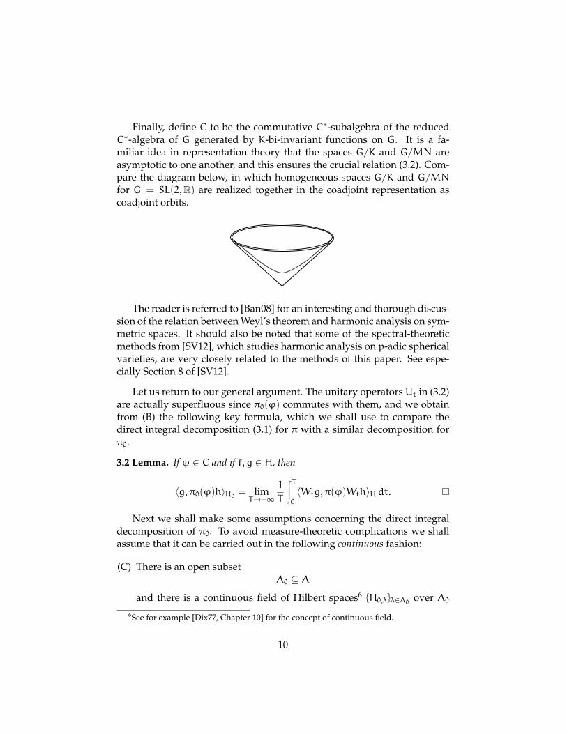
Finally, define C to be the commutative C∗-subalgebra of the reducedC∗-algebra of G generated by K-bi-invariant functions on G. It is a fa-miliar idea in representation theory that the spaces G/K and G/MN areasymptotic to one another, and this ensures the crucial relation (3.2). Com-pare the diagram below, in which homogeneous spaces G/K and G/MNfor G = SL(2,R) are realized together in the coadjoint representation ascoadjoint orbits.

The reader is referred to [Ban08] for an interesting and thorough discus-sion of the relation between Weyl’s theorem and harmonic analysis on sym-metric spaces. It should also be noted that some of the spectral-theoreticmethods from [SV12], which studies harmonic analysis on p-adic sphericalvarieties, are very closely related to the methods of this paper. See espe-cially Section 8 of [SV12].

Let us return to our general argument. The unitary operatorsUt in (3.2)are actually superfluous since π0(ϕ) commutes with them, and we obtainfrom (B) the following key formula, which we shall use to compare thedirect integral decomposition (3.1) for π with a similar decomposition forπ0.

3.2 Lemma. If ϕ ∈ C and if f, g ∈ H, then

〈g, π0(ϕ)h〉H0 = limT→+∞ 1

T

∫ T0

〈Wtg, π(ϕ)Wth〉H dt.

Next we shall make some assumptions concerning the direct integraldecomposition of π0. To avoid measure-theoretic complications we shallassume that it can be carried out in the following continuous fashion:

(C) There is an open subsetΛ0 ⊆ Λ

and there is a continuous field of Hilbert spaces6 {H0,λ}λ∈Λ0 over Λ06See for example [Dix77, Chapter 10] for the concept of continuous field.

10

with constant and finite fiber dimension that decomposes the repre-sentation π0 in the following sense. There is a dense subspace

H0 ⊆ H0

and there are linear maps

ε0,λ : H0 −→ H0,λ,

defined for every λ ∈ Λ0, that carry the elements of H0 to a total family7

of continuous sections of {H0,λ}. Moreover there is a Borel measure µ0on Λ0 for which⟨

h, π0(ϕ)g⟩H0

=

∫Λ0

⟨ε0,λ(h), ε0,λ(g)

⟩H0,λ

ϕ(λ)dµ0(λ)

for every ϕ ∈ C and all h, g ∈ H0. Part of the assumption here isthat the integrand, which is a continuous function on Λ0, is in fact anintegrable function.

We shall also assume compatibility between our continuous field andthe one-parameter unitary group action on H0:

(D) The one-parameter unitary group {Ut} on H0 maps the subspace H0into itself. Moreover the continuous field {H0,λ}λ∈Λ0 carries a continu-ous, unitary action of R such that

ε0,λ(Uth) = Utε0,λ(h)

for every h ∈ H0 and every λ ∈ Λ0 (we shall use the same symbol Utfor the unitary action on the continuous field).

Underlying the continuous field {H0,λ}λ∈Λ0 there is a measurable field ofHilbert spaces (for which a section of {H0,λ}λ∈Λ0 is by definition measurableif its inner product with any continuous section is a measurable function),and the assumption (C) gives a direct integral decomposition

(3.3) H0 ∼=

∫Λ0

H0,λ dµ0(λ)

of the representation π0.

7This means that the values of these sections at any point λ span H0,λ; see [Dix77, Defi-nition 10.2.1].

11

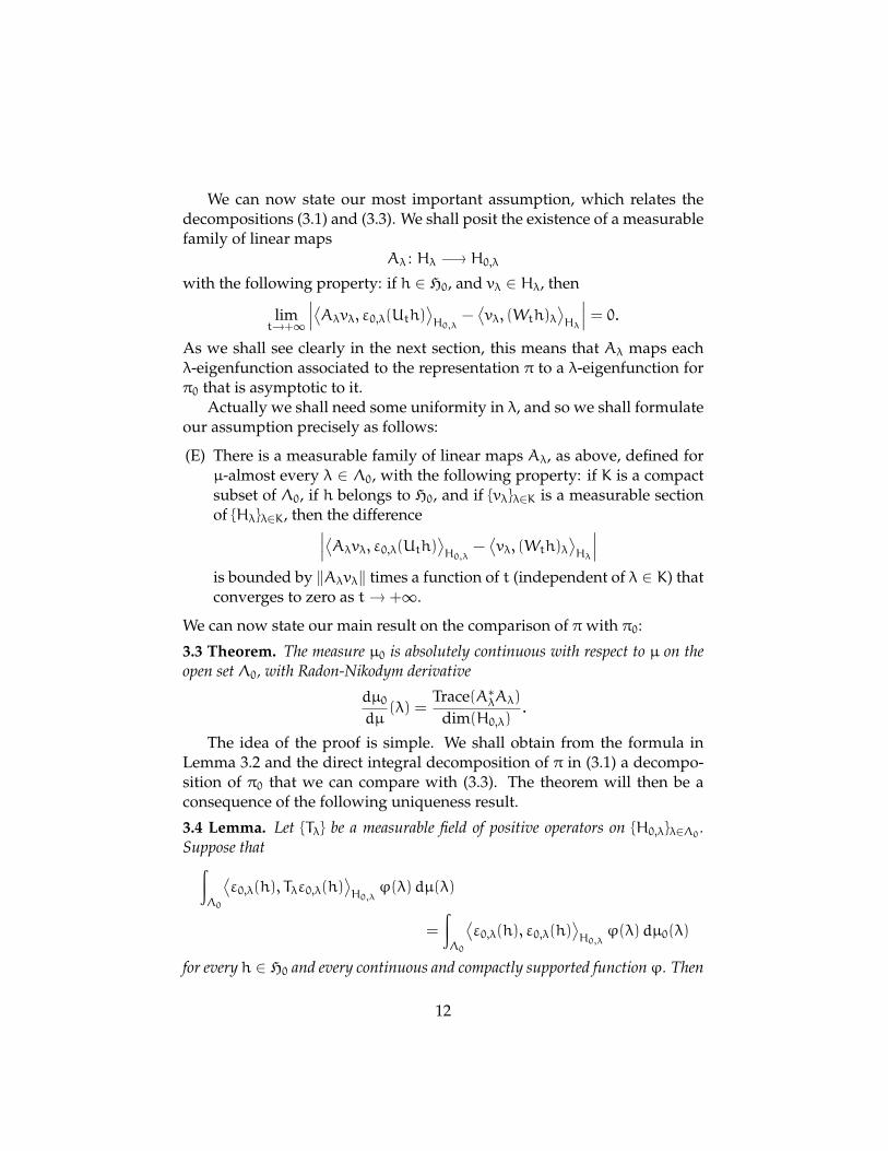
We can now state our most important assumption, which relates thedecompositions (3.1) and (3.3). We shall posit the existence of a measurablefamily of linear maps

Aλ : Hλ −→ H0,λ

with the following property: if h ∈ H0, and vλ ∈ Hλ, then

limt→+∞

∣∣∣⟨Aλvλ, ε0,λ(Uth)⟩H0,λ − ⟨vλ, (Wth)λ⟩Hλ

∣∣∣ = 0.As we shall see clearly in the next section, this means that Aλ maps eachλ-eigenfunction associated to the representation π to a λ-eigenfunction forπ0 that is asymptotic to it.

Actually we shall need some uniformity in λ, and so we shall formulateour assumption precisely as follows:

(E) There is a measurable family of linear maps Aλ, as above, defined forµ-almost every λ ∈ Λ0, with the following property: if K is a compactsubset of Λ0, if h belongs to H0, and if {vλ}λ∈K is a measurable sectionof {Hλ}λ∈K, then the difference∣∣∣⟨Aλvλ, ε0,λ(Uth)⟩H0,λ − ⟨vλ, (Wth)λ

⟩Hλ

∣∣∣is bounded by ‖Aλvλ‖ times a function of t (independent of λ ∈ K) thatconverges to zero as t→ +∞.

We can now state our main result on the comparison of πwith π0:

3.3 Theorem. The measure µ0 is absolutely continuous with respect to µ on theopen set Λ0, with Radon-Nikodym derivative

dµ0dµ

(λ) =Trace(A∗λAλ)

dim(H0,λ).

The idea of the proof is simple. We shall obtain from the formula inLemma 3.2 and the direct integral decomposition of π in (3.1) a decompo-sition of π0 that we can compare with (3.3). The theorem will then be aconsequence of the following uniqueness result.

3.4 Lemma. Let {Tλ} be a measurable field of positive operators on {H0,λ}λ∈Λ0 .Suppose that∫

Λ0

⟨ε0,λ(h), Tλε0,λ(h)

⟩H0,λ

ϕ(λ)dµ(λ)

=

∫Λ0

⟨ε0,λ(h), ε0,λ(h)

⟩H0,λ

ϕ(λ)dµ0(λ)

for every h ∈ H0 and every continuous and compactly supported functionϕ. Then

12

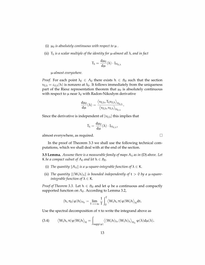
(i) µ0 is absolutely continuous with respect to µ .

(ii) Tλ is a scalar multiple of the identity for µ-almost all λ, and in fact

Tλ =dµ0dµ

(λ) · IH0,λ

µ-almost everywhere.

Proof. For each point λ0 ∈ Λ0 there exists h ∈ H0 such that the sectionv0,λ = ε0,λ(h) is nonzero at λ0. It follows immediately from the uniquenesspart of the Riesz representation theorem that µ0 is absolutely continuouswith respect to µ near λ0 with Radon-Nikodym derivative

dµ0dµ

(λ) =

⟨v0,λ, Tλv0,λ

⟩H0,λ⟨

v0,λ, v0,λ⟩H0,λ

.

Since the derivative is independent of {v0,λ} this implies that

Tλ =dµ0dµ

(λ) · IH0,λ ,

almost everywhere, as required.

In the proof of Theorem 3.3 we shall use the following technical com-putations, which we shall deal with at the end of the section.

3.5 Lemma. Assume there is a measurable family of mapsAλ as in (D) above. LetK be a compact subset of Λ0 and let h ∈ H0.

(i) The quantity ‖Aλ‖ is a µ-square-integrable function of λ ∈ K.

(ii) The quantity ‖(Wth)λ‖ is bounded independently of t > 0 by a µ-square-integrable function of λ ∈ K.

Proof of Theorem 3.3. Let h ∈ H0 and let ϕ be a continuous and compactlysupported function on Λ0. According to Lemma 3.2,

〈h, π0(ϕ)h〉H0 = limT→+∞ 1

T

∫ T0

⟨Wth, π(ϕ)Wth

⟩Hdt.

Use the spectral decomposition of π to write the integrand above as

(3.4)⟨Wth, π(ϕ)Wth

⟩H=

∫supp(ϕ)

⟨(Wth)λ, (Wth)λ

⟩Hλϕ(λ)dµ(λ).

13

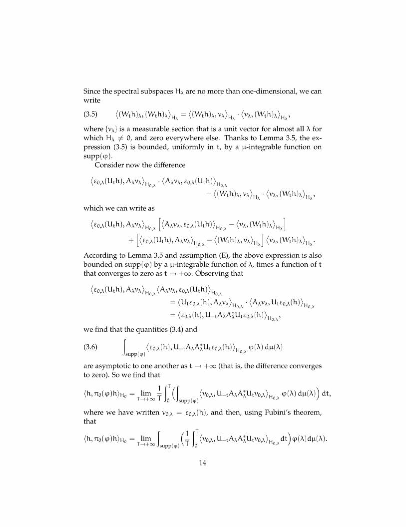
Since the spectral subspaces Hλ are no more than one-dimensional, we canwrite

(3.5)⟨(Wth)λ, (Wth)λ

⟩Hλ

=⟨(Wth)λ, vλ

⟩Hλ·⟨vλ, (Wth)λ

⟩Hλ,

where {vλ} is a measurable section that is a unit vector for almost all λ forwhich Hλ 6= 0, and zero everywhere else. Thanks to Lemma 3.5, the ex-pression (3.5) is bounded, uniformly in t, by a µ-integrable function onsupp(ϕ).

Consider now the difference⟨ε0,λ(Uth), Aλvλ

⟩H0,λ·⟨Aλvλ, ε0,λ(Uth)

⟩H0,λ

−⟨(Wth)λ, vλ

⟩Hλ·⟨vλ, (Wth)λ

⟩Hλ,

which we can write as⟨ε0,λ(Uth), Aλvλ

⟩H0,λ

[⟨Aλvλ, ε0,λ(Uth)

⟩H0,λ

−⟨vλ, (Wth)λ

⟩Hλ

]+[⟨ε0,λ(Uth), Aλvλ

⟩H0,λ

−⟨(Wth)λ, vλ

⟩Hλ

] ⟨vλ, (Wth)λ

⟩Hλ.

According to Lemma 3.5 and assumption (E), the above expression is alsobounded on supp(ϕ) by a µ-integrable function of λ, times a function of tthat converges to zero as t→ +∞. Observing that⟨ε0,λ(Uth), Aλvλ

⟩H0,λ

⟨Aλvλ, ε0,λ(Uth)

⟩H0,λ

=⟨Utε0,λ(h), Aλvλ

⟩H0,λ·⟨Aλvλ, Utε0,λ(h)

⟩H0,λ

=⟨ε0,λ(h), U−tAλA

∗λUtε0,λ(h)

⟩H0,λ

,

we find that the quantities (3.4) and

(3.6)∫

supp(ϕ)

⟨ε0,λ(h), U−tAλA

∗λUtε0,λ(h)

⟩H0,λ

ϕ(λ)dµ(λ)

are asymptotic to one another as t→ +∞ (that is, the difference convergesto zero). So we find that

〈h, π0(ϕ)h〉H0 = limT→+∞ 1

T

∫ T0

(∫supp(ϕ)

⟨v0,λ, U−tAλA

∗λUtv0,λ

⟩H0,λ

ϕ(λ)dµ(λ))dt,

where we have written v0,λ = ε0,λ(h), and then, using Fubini’s theorem,that

〈h, π0(ϕ)h〉H0 = limT→+∞

∫supp(ϕ)

( 1T

∫ T0

⟨v0,λ, U−tAλA

∗λUtv0,λ

⟩H0,λ

dt)ϕ(λ)dµ(λ).

14

The term in parentheses is bounded by an integrable function on supp(ϕ)that is independent of t. Therefore the dominated convergence theoremallows us to interchange the limit as T → +∞ and the integral over supp(ϕ)to obtain

〈h, π0(ϕ)h〉H0 =∫Λ0

⟨v0,λ,Av

[AλA

∗λ

]v0,λ⟩H0,λ

ϕ(λ)dµ(λ),

where

Av[AλA

∗λ

]= limT→∞ 1

T

∫ T0

U−tAλA∗λUt dt

(since we are dealing here with operators on the finite-dimensional spaceH0,λ the limit certainly exists).

We can now apply Lemma 3.4, which tells us that the operator Av[AλA∗λ]is a scalar multiple of the identity for µ-almost-all λ. The computation

Trace(Av[AλA

∗λ

])= Trace(AλA∗λ) = Trace(A∗λAλ),

determines the multiple, and the theorem follows.

The theorem we have just proved gives a formula for the measure µ0 interms of the measure µ. But since our goal is to obtain information aboutthe measure µ, we should invert this formula, and for this purpose we shallmake a final assumption:

(F) The operators Aλ are nonzero for every λ ∈ Λ0.

With this, the following is an immediate consequence of Theorem 3.3:

3.6 Theorem. The measue µ is absolutely continuous with respect to µ0 on Λ0,and the Radon-Nikodym derivative of µ with respect to µ0 is

dµ

dµ0(λ) =

dim(H0,λ)

Trace(A∗λAλ)

on Λ0.

Proof of Lemma 3.5. Since the continuous field {H0,λ}λ∈K has finite and con-stant fiber dimension, and since the sections associated to elements of H0constitute a total set, there is a finite set of elements {hj} in H0 such that

‖wλ‖H0,λ ≤∑j

∣∣⟨wλ, ε0,λ(hj)⟩H0,λ∣∣15

for all λ ∈ K and all wλ ∈ H0,λ. Applying this inequality to wλ of the formU−tAλvλ we get

‖Aλvλ‖H0,λ ≤∑j

∣∣⟨Aλvλ, ε0,λ(Uthj)⟩H0,λ∣∣for all t > 0, all λ ∈ K and all vλ ∈ Hλ. Now it follows from assumption (E)that there is some function f(t) that converges to zero as t→ +∞ such that∑

j

∣∣⟨Aλvλ, ε0,λ(Uthj)⟩H0,λ∣∣ ≤∑j

∣∣⟨vλ, (Wthj)λ⟩Hλ

∣∣+ ‖Aλvλ‖H0,λ · f(t)for all t > 0, all λ ∈ K and all vλ ∈ Hλ. Rearrange this as

(3.7) ‖Aλvλ‖H0,λ(1− f(t)) ≤∑j

∣∣⟨vλ, (Wthj)λ⟩Hλ

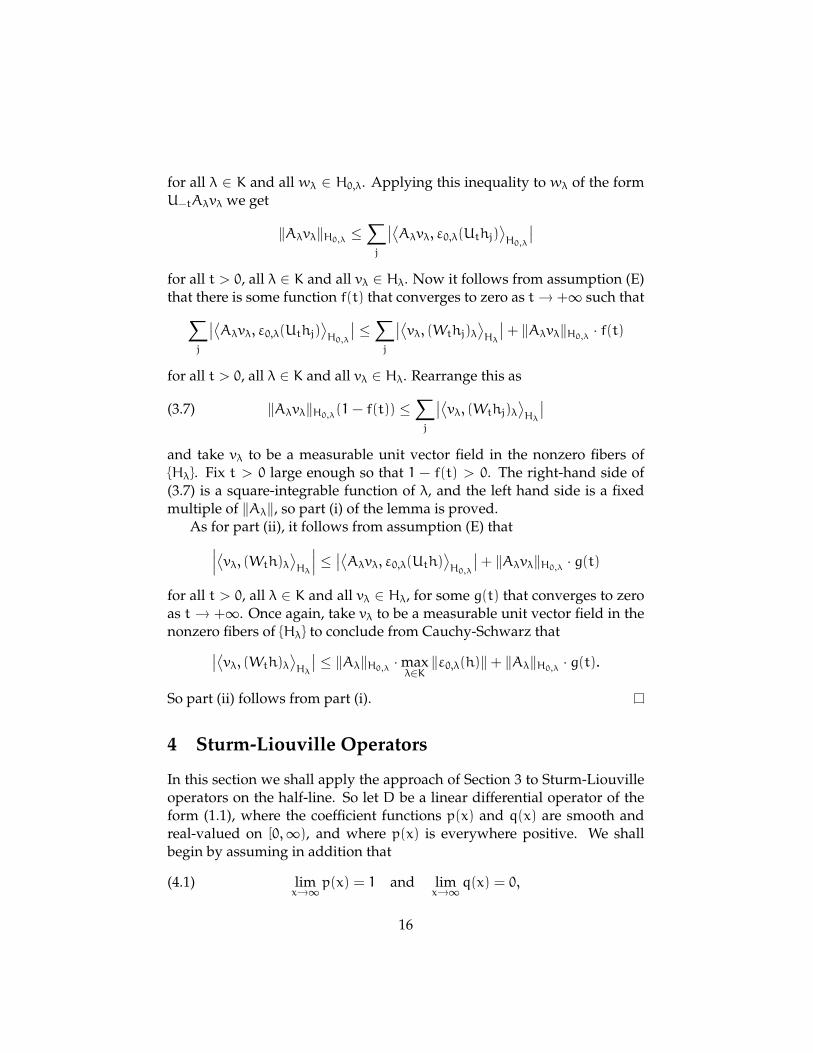
∣∣and take vλ to be a measurable unit vector field in the nonzero fibers of{Hλ}. Fix t > 0 large enough so that 1 − f(t) > 0. The right-hand side of(3.7) is a square-integrable function of λ, and the left hand side is a fixedmultiple of ‖Aλ‖, so part (i) of the lemma is proved.

As for part (ii), it follows from assumption (E) that∣∣∣⟨vλ, (Wth)λ⟩Hλ

∣∣∣ ≤ ∣∣⟨Aλvλ, ε0,λ(Uth)⟩H0,λ∣∣+ ‖Aλvλ‖H0,λ · g(t)for all t > 0, all λ ∈ K and all vλ ∈ Hλ, for some g(t) that converges to zeroas t → +∞. Once again, take vλ to be a measurable unit vector field in thenonzero fibers of {Hλ} to conclude from Cauchy-Schwarz that∣∣⟨vλ, (Wth)λ

⟩Hλ

∣∣ ≤ ‖Aλ‖H0,λ ·maxλ∈K‖ε0,λ(h)‖+ ‖Aλ‖H0,λ · g(t).

So part (ii) follows from part (i).

4 Sturm-Liouville Operators

In this section we shall apply the approach of Section 3 to Sturm-Liouvilleoperators on the half-line. So let D be a linear differential operator of theform (1.1), where the coefficient functions p(x) and q(x) are smooth andreal-valued on [0,∞), and where p(x) is everywhere positive. We shallbegin by assuming in addition that

(4.1) limx→∞p(x) = 1 and lim

x→∞q(x) = 0,16

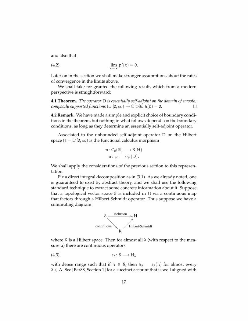
and also that

(4.2) limx→∞p ′(x) = 0.

Later on in the section we shall make stronger assumptions about the ratesof convergence in the limits above.

We shall take for granted the following result, which from a modernperspective is straightforward:

4.1 Theorem. The operatorD is essentially self-adjoint on the domain of smooth,compactly supported functions h : [0,∞) → C with h(0) = 0.

4.2 Remark. We have made a simple and explicit choice of boundary condi-tions in the theorem, but nothing in what follows depends on the boundaryconditions, as long as they determine an essentially self-adjoint operator.

Associated to the unbounded self-adjoint operator D on the Hilbertspace H = L2[0,∞) is the functional calculus morphism

π : C0(R) −→ B(H)

π : ϕ 7−→ ϕ(D).

We shall apply the considerations of the previous section to this represen-tation.

Fix a direct integral decomposition as in (3.1). As we already noted, oneis guaranteed to exist by abstract theory, and we shall use the followingstandard technique to extract some concrete information about it. Supposethat a topological vector space S is included in H via a continuous mapthat factors through a Hilbert-Schmidt operator. Thus suppose we have acommuting diagram

Sinclusion //

continuous ��

H

KHilbert-Schmidt

??

where K is a Hilbert space. Then for almost all λ (with respect to the mea-sure µ) there are continuous operators

(4.3) ελ : S −→ Hλ

with dense range such that if h ∈ S, then hλ = ελ(h) for almost everyλ ∈ Λ. See [Ber88, Section 1] for a succinct account that is well aligned with

17

the outlook of this paper. Or see the Fundamental Theorem in [Mau67,Chapter VII, Section 1].

In our case we can take S = C∞c [0,∞) (compare [Ber88, Section 1,

Lemma 2.3]). Since the maps (4.3) have dense range for almost every λ,the adjoint maps

(4.4) ε∗λ : H∗λ −→ S∗

are almost always injective. This leads to a description of Hλ as a space ofeigenfunctions, based on the fact that

H∗λ∼= Hλ.

In fact, if h is smooth and compactly supported in the open half-line (0,∞),while g ∈ S, then

〈Dh, g〉 = 〈h,Dg〉,

and as a resultDε∗λ(g) = λε

∗λ(g)

in the sense of distributions on (0,∞), for almost all λ ∈ Λ. So for almostall λ, the map ε∗λ embeds H∗λ into the space S∗λ of λ-eigendistributions forD. By linear ODE theory S∗λ consists of smooth functions on [0,∞) and istwo-dimensional.

4.3 Lemma. For almost every λ ∈ Λ the adjoint maps (4.4) embed H∗λ into thespace of smooth function solutions in S∗ of the differential equation DFλ = λFλthat satisfy the boundary condition Fλ(0) = 0.

Proof. If h ∈ S, and if g is in the domain ofD (by which we mean, both hereand subsequently, the domain of the self-adjoint closure of D), then

(4.5) 〈ελ(Dh), gλ〉Hλ − 〈ελ(h), (Dg)λ〉Hλ

=

∫∞0

(Dh)(x)Gλ(x)dx−

∫∞0

h(x)(DGλ)(x)dx

= p(0)(h ′(0)Gλ(0) − h(0)G

′λ(0)

)(c.f. (2.6)). Here Gλ = ε∗λgλ. The top expression in (4.5) is an integrablefunction of λ, and therefore so is the bottom.

If we choose h ∈ S so that h(0) = 0, then h ∈ dom(D). In this case thetop expression in (4.5) integrates to zero for µ-almost all λ. So if we chooseh so that in addition h ′(0) 6= 0, then we find that Gλ(0) is an integrable

18

function of λ, and it integrates to zero. Replacing g ∈ dom(D) with ϕ(D)g,where ϕ is any bounded Borel function, we get∫

Λ0

Gλ(0)ϕ(λ)dµ(λ) = 0,

and therefore Gλ(0) = 0 for almost every λ. It follows that for almost everyλ the image of the adjoint map (4.4) is contained in the one-dimensionalspace of smooth λ-eigenfunctions forD that satisfy the boundary conditionGλ(0) = 0, as required.

Of course there is a precisely one-dimensional space of eigenfunctionsFλ for which Fλ(0) = 0, and so it follows immediately from the lemma thatdimHλ ≤ 1 for µ-almost every λ ∈ Λ, as required in assumption (A) fromthe previous section.

Next we define H0 = L2(−∞,∞) which obviously contains H as aclosed subspace; we shall denote by

W : H0 −→ H

the orthogonal projection. Define

D0 = −d2

dx2,

which we shall treat as an essentially self-adjoint operator on the Hilbertspace H0 with domain the smooth, compactly supported functions on theline, and define

π0 : C0(R) −→ B(H0)

by π0(ϕ) = ϕ(D0). Define Ut : H0 → H0 to be the translation operator

(Uth)(x) = h(x−t).

Obviously eachϕ(D0) commutes with eachUt. The following computationchecks assumption (B) from the previous section.

4.4 Lemma. If ϕ ∈ C0(R) and if g, h ∈ L2(0,∞), then

limt→+∞

[⟨Utg,ϕ(D)Uth

⟩L2(0,∞)

−⟨Utg,ϕ(D0)Uth

⟩L2(−∞,∞)

]= 0.

Proof. Much more is true, namely that

(4.6) limt→+∞

∥∥ϕ(D)Ut −ϕ(D0)Ut∥∥B(H,H0)

= 0

19

for everyϕ ∈ C0(R). To prove this, observe first that the set of allϕ ∈ C0(R)satisfying (4.6) is a norm-closed subalgebra of C0(R), so it suffices to showthat the resolvent functions ϕ(λ) = (λ± i)−1 belong to it.

Let ψ be a smooth function on R that is identically zero in a neigh-borhood of (−∞, 0] and identically one in a neighborhood of [1,∞), andfor t > 0 let Mt be the bounded operator of pointwise multiplication byλ 7→ ψ(t−1λ) (it is an operator on H0 whose range lies in H). Then

Ut =MtUt : H −→ H0

and by standard Sobolev space estimates (the basic elliptic estimate, ap-plied to D0)

limt→+∞ ‖Mtϕ(D0) −ϕ(D0)Mt‖ = 0

for ϕ(λ) = (λ± i)−1, or indeed for every ϕ ∈ C0(R). Now

ϕ(D)Ut −ϕ(D0)Ut = ϕ(D)MtUt −ϕ(D0)MtUt

as operators from H to H0, and the right-hand side is asymptotic in normto

ϕ(D)MtUt −Mtϕ(D0)Ut.

For the particular case where ϕ(λ) = (λ± i)−1, the above may be expressedas

(4.7) ϕ(D)[MtD0 −DMt

]ϕ(D0)Ut.

The expression in the middle is, for each t > 0, a second order differentialoperator

at(x)d2

dx2+ bt(x)

d

dx+ ct(x)

on the line and as t → +∞ the coefficient functions converge uniformlyto zero. So by the basic estimates (4.7) is a bounded operator whose normconverges uniformly to zero as t tends to infinity.

The spectral theory of the operatorD0 is of course easily obtained fromFourier theory. Let

Λ0 = (0,∞),

and for λ ∈ Λ0 define H0,λ to be the two-dimensional vector space of func-tions on the line spanned by ei

√λx and e−i

√λx. Equip H0,λ with the inner

product that makes these two functions an orthonormal basis. The family

20

{H0,λ}λ>0 obviously forms a continuous field of Hilbert spaces over Λ0 withconstant and finite fiber dimension. Now let H0 be space of smooth andcompactly supported functions in H0. The Fourier transform

h(ξ) =

∫∞−∞ h(x)e−iξx dx

associates to each h ∈ H0 a continuous section {ε0,λ(h)} of the continuousfield, namely

ε0,λ(h) = h(√λ)ei

√λx + h(−

√λ)e−i

√λx.

We obtain a total family of sections, and it follows from Plancherel’s for-mula that

〈h,ϕ(D0)g〉L2(−∞,∞) =

∫Λ0

〈ε0,λ(h), ε0,λ(g)〉H0,λ ϕ(λ)dµ0(λ),

where

(4.8) dµ0(λ) =1

4π

dλ√λ.

This takes care of assumption (C), and moreover assumption (D) is a simpleconsequence Fourier theory, too.

Finally, we need to analyze the asymptotics of the λ-eigenfunctions ofD. Our method is essentially the same as Weyl’s [Wey10], and it is in anycase standard (moreover it is perhaps worth noting that in the simple casewhere the coefficients of D are eventually constant, nothing from here upto the formulation of Theorem 4.8 is needed at all).

4.5 Lemma. Suppose that a smooth function u : [0,∞) → Cn is a solution of thedifferential equation

u ′(x) = Cu(x) +Q(x)u(x)

where C is a constant n×n matrix and Q is a smooth n×n matrix-valued func-tion. Let

(4.9) k(x) =

∫∞x

‖ exp(−xC)Q(x) exp(xC)‖dx

and assume that k(0) <∞. If

s(x) = exp(−xC)u(x)

then the limits(∞) = lim

x→+∞ s(x)21

exists. Moreover,

(4.10) ‖s(∞) − s(x)‖ ≤ constant · k(x) · ‖s(∞)‖,

where the constant can be chosen to be a continuous function of k(0). In particular,if the limit s(∞) is zero, then s(x) is identically zero.

4.6 Remark. Since all norms on finite-dimensional spaces are equivalent,we can choose any norm in (4.9) and below. We shall choose the Hilbert-Schmidt norm

‖T‖2 = Trace(T∗T).

This is a submultiplicative norm, and it has the advantage over, for exam-ple, the operator norm, of being a smooth function on the space of nonzeromatrices.

Proof of the Lemma. Consider the linear differential equation

U ′(x) = CU(x) +Q(x)U(x)

in which U(x) is a smooth, n×n matrix-valued function. There exists aunique solution for the initial condition

U(0) = I,

and it is defined for all x. Moreover each U(x) is invertible: the inversematrices can be obtained by solving the linear differential equation

V ′(x) = −V(x)C−U(x)Q(x)

with initial condition V(0) = I. If we write

S(x) = exp(−xC)U(x),

thenS ′(x) = exp(−xC)Q(x) exp(xC)S(x),

and so of course

(4.11) ‖S ′(x)‖ ≤ ‖ exp(−xC)Q(x) exp(xC)‖ · ‖S(x)‖.

This, together with the simple inequality∣∣∣ ddx‖S(x)‖

∣∣∣ ≤ ‖S ′(x)‖22

gives us the estimate

(4.12)∣∣∣ ddx

log ‖S(x)‖∣∣∣ ≤ ‖ exp(−xC)Q(x) exp(xC)‖.

The integrability hypothesis of the lemma now implies that

supx∈[0,∞)

log ‖S(x)‖ <∞,and therefore

(4.13) supx∈[0,∞)

‖S(x)‖ <∞.Both suprema are bounded by a continuous function of k(0). Returning to(4.11), it follows from (4.13) that

(4.14) ‖S ′(x)‖ ≤ constant · ‖ exp(−xC)Q(x) exp(xC)‖,

where the constant can be chosen to be a continuous function of k(0). Soby applying the integrability hypothesis a second time we find that S(x)converges to a limit S(∞) as x tends to infinity.

The limit S(∞) is an invertible matrix. Indeed we can apply the argu-ment we’ve just given to the matrix-valued function

T(x) = S(x)−1 = U(x)−1 exp(xC),

in place of S(x). The function T(x) is a solution of the differential equation

T ′(x) = −T(x) exp(−xC)Q(x) exp(xC),

and the argument above shows that T(x) converges to a limit as x tends toinfinity, and is bounded by a continuous function of k(0). And of course

limx→∞ T(x) · lim

x→∞S(x) = limx→∞ T(x)S(x) = I.

To complete the proof, it follows from the uniqueness of solutions prop-erty for ODE’s that

u(x) = U(x)u(0),

so that

s(x) = exp(−xC)u(x) = exp(−xC)U(x)u(0) = S(x)u(0).

23

So the limit s(∞) exists. As for (4.10), we can write

‖s(∞) − s(x)‖ ≤ ‖S(∞)‖ · ‖I− T(∞)S(x)‖ · ‖u(0)‖,

and then estimate the middle norm on the right-hand side by∫∞x

‖T(∞)‖‖S ′(x)‖dx.

From (4.14) we obtain

‖s(∞) − s(x)‖ ≤ constant · k(x) · ‖u(0)‖.

Since u(0) = T(∞)s(∞), we obtain

‖s(∞) − s(x)‖ ≤ constant · k(x) · ‖s(∞)‖,

for a constant that is a continuous function of k(0), as required.

Let us apply this to the Sturm-Liouville eigenvalue equation. If λ ∈ Cand if Fλ is any λ-eigenfunction for D, then the vector-valued function

(4.15) uλ(x) =

[p(x)F ′λ(x)Fλ(x)

]is a solution of the differential equation

(4.16) u ′(x) = Cλu(x) +Q(x)u(x),

where

(4.17) Cλ =

[0 1

−λ 0

]and Q(x) =

[0 q(x)

1− p(x)−1 0

].

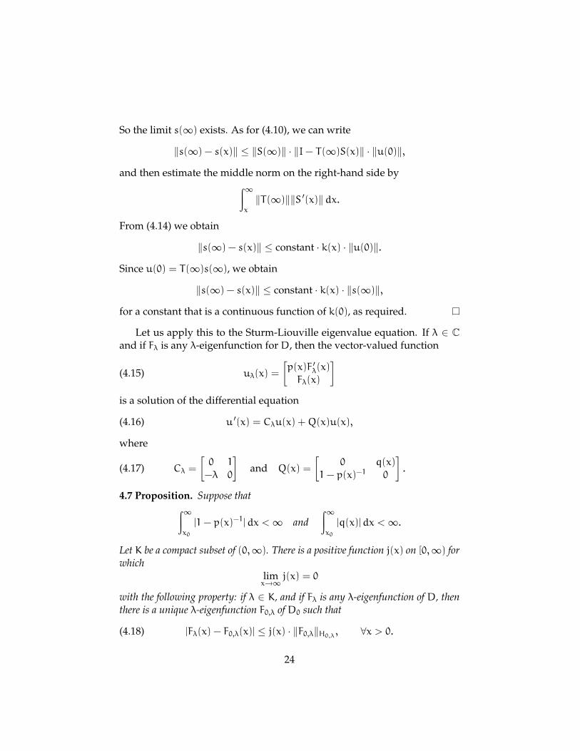
4.7 Proposition. Suppose that∫∞x0

|1− p(x)−1|dx <∞ and∫∞x0

|q(x)|dx <∞.Let K be a compact subset of (0,∞). There is a positive function j(x) on [0,∞) forwhich

limx→∞ j(x) = 0

with the following property: if λ ∈ K, and if Fλ is any λ-eigenfunction of D, thenthere is a unique λ-eigenfunction F0,λ of D0 such that

(4.18) |Fλ(x) − F0,λ(x)| ≤ j(x) · ‖F0,λ‖H0,λ , ∀x > 0.

24

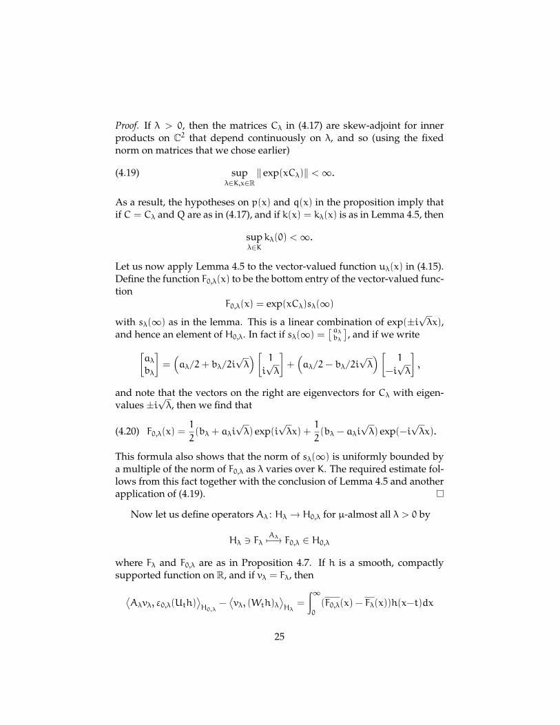
Proof. If λ > 0, then the matrices Cλ in (4.17) are skew-adjoint for innerproducts on C2 that depend continuously on λ, and so (using the fixednorm on matrices that we chose earlier)

(4.19) supλ∈K,x∈R

‖ exp(xCλ)‖ <∞.As a result, the hypotheses on p(x) and q(x) in the proposition imply thatif C = Cλ andQ are as in (4.17), and if k(x) = kλ(x) is as in Lemma 4.5, then

supλ∈K

kλ(0) <∞.Let us now apply Lemma 4.5 to the vector-valued function uλ(x) in (4.15).Define the function F0,λ(x) to be the bottom entry of the vector-valued func-tion

F0,λ(x) = exp(xCλ)sλ(∞)

with sλ(∞) as in the lemma. This is a linear combination of exp(±i√λx),

and hence an element of H0,λ. In fact if sλ(∞) =[ aλbλ

], and if we write[

aλbλ

]=(aλ/2+ bλ/2i

√λ)[ 1

i√λ

]+(aλ/2− bλ/2i

√λ)[ 1

−i√λ

],

and note that the vectors on the right are eigenvectors for Cλ with eigen-values ±i

√λ, then we find that

(4.20) F0,λ(x) =1

2(bλ + aλi

√λ) exp(i

√λx) +

1

2(bλ − aλi

√λ) exp(−i

√λx).

This formula also shows that the norm of sλ(∞) is uniformly bounded bya multiple of the norm of F0,λ as λ varies over K. The required estimate fol-lows from this fact together with the conclusion of Lemma 4.5 and anotherapplication of (4.19).

Now let us define operators Aλ : Hλ → H0,λ for µ-almost all λ > 0 by

Hλ 3 FλAλ7−→ F0,λ ∈ H0,λ

where Fλ and F0,λ are as in Proposition 4.7. If h is a smooth, compactlysupported function on R, and if vλ = Fλ, then

⟨Aλvλ, ε0,λ(Uth)

⟩H0,λ

−⟨vλ, (Wth)λ

⟩Hλ

=

∫∞0

(F0,λ(x) − Fλ(x))h(x−t)dx

25

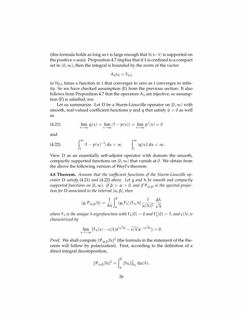
(this formula holds as long as t is large enough that h(x−t) is supported onthe positive x-axis). Proposition 4.7 implies that if λ is confined to a compactset in (0,∞), then the integral is bounded by the norm of the vector

Aλvλ = F0,λ

in H0,λ times a function in t that converges to zero as t converges to infin-ity. So we have checked assumption (E) from the previous section. It alsofollows from Proposition 4.7 that the operatorsAλ are injective, so assump-tion (F) is satisfied, too.

Let us summarize. Let D be a Sturm-Liouville operator on [0,∞) withsmooth, real-valued coefficient functions p and q that satisfy p > 0 as wellas

(4.21) limx→∞q(x) = lim

x→∞(1− p(x)) = limx→∞p ′(x) = 0

and

(4.22)∫∞1

|1− p(x)−1|dx <∞ ∫∞1

|q(x)|dx <∞.View D as an essentially self-adjoint operator with domain the smooth,compactly supported functions on [0,∞) that vanish at 0. We obtain fromthe above the following version of Weyl’s theorem:

4.8 Theorem. Assume that the coefficient functions of the Sturm-Liouville op-erator D satisfy (4.21) and (4.22) above. Let g and h be smooth and compactlysupported functions on [0,∞). If β > α > 0, and if P[α,β] is the spectral projec-tion for D associated to the interval [α,β], then

〈g, P[α,β]h〉 =1

4π

∫βα

〈g, Fλ〉〈Fλ, h〉1

|c(λ)|2dλ√λ

where Fλ is the unique λ-eigenfunction with Fλ(0) = 0 and F ′λ(0) = 1, and c(λ) ischaracterized by

limx→+∞

(Fλ(x) − c(λ)e

i√λx − c(λ)e−i

√λx)= 0.

Proof. We shall compute ‖P[α,β]h‖2 (the formula in the statement of the the-orem will follow by polarization). First, according to the definition of adirect integral decomposition,

‖P[α,β]h‖2 =∫βα

‖hλ‖2Hλ dµ(λ).

26

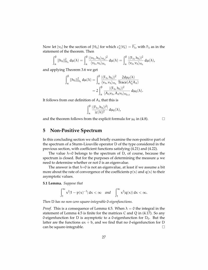
Now let {vλ} be the section of {Hλ} for which ε∗λ(vλ) = Fλ, with Fλ as in thestatement of the theorem. Then∫β

α

‖hλ‖2Hλ dµ(λ) =∫βα

|〈vλ, hλ〉Hλ |2

〈vλ, vλ〉Hλdµ(λ) =

∫βα

|〈Fλ, hλ〉|2

〈vλ, vλ〉Hλdµ(λ),

and applying Theorem 3.6 we get∫βα

‖hλ‖2Hλ dµ(λ) =∫βα

|〈Fλ, hλ〉|2

〈vλ, vλ〉Hλ2dµ0(λ)

Trace(A∗λAλ)

= 2

∫βα

|〈Fλ, hλ〉|2

〈Aλvλ, Aλvλ〉H0,λdµ0(λ).

It follows from our definition of Aλ that this is∫βα

|〈Fλ, hλ〉|2||c(λ)|2

dµ0(λ),

and the theorem follows from the explicit formula for µ0 in (4.8).

5 Non-Positive Spectrum

In this concluding section we shall briefly examine the non-positive part ofthe spectrum of a Sturm-Liouville operatorD of the type considered in theprevious section, with coefficient functions satisfying (4.21) and (4.22).

The value λ=0 belongs to the spectrum of D, of course, because thespectrum is closed. But for the purposes of determining the measure µ weneed to determine whether or not 0 is an eigenvalue.

The answer is that λ=0 is not an eigenvalue, at least if we assume a bitmore about the rate of convergence of the coefficients p(x) and q(x) to theirasymptotic values.

5.1 Lemma. Suppose that∫∞1

x2|1− p(x)−1|dx <∞ and∫∞1

x2|q(x)|dx <∞.Then D has no non-zero square-integrable 0-eigenfunctions.

Proof. This is a consequence of Lemma 4.5. When λ = 0 the integral in thestatement of Lemma 4.5 is finite for the matrices C and Q in (4.17). So any0-eigenfunction for D is asymptotic to a 0-eigenfunction for D0. But thelatter are the functions ax + b, and we find that no 0-eigenfunction for Dcan be square-integrable.

27

Let us consider now the negative part of the spectrum of D. The ar-gument below is not optimal,8 but it uses the same ideas we have alreadydeveloped to handle the continuous spectrum. Moreover it is adequate tohandle the operators that arise in harmonic analysis.

5.2 Lemma. If we assume that∫∞1

eαx|1− p(x)−1|dx <∞ and∫∞1

eαx|q(x)|dx <∞.for some α > 0, then λ=0 is not a limit point of the set of eigenvalues of theself-adjoint Hilbert space operator D.

Proof. For every λ ∈ C the matrix Cλ in (4.17) satisfies C2λ = −λI, and there-fore

(5.1) exp(xCλ) = cosh(x√λ)I+

sinh(x√λ)√

λCλ

for any square root of λ. It follows from this that if ε > δ > 0, then

(5.2) |λ| ≤ δ ⇒ ‖ exp(xCλ)‖ ≤ constant · eεx

for all x and some constant independent of λ and x. Now choose ε = α/4.The estimate (5.2) and Lemma 4.5 imply that for uλ(x) as in (4.15) the limit

wλ := limx→∞ exp(−xCλ)uλ(x)

exists whenever |λ| ≤ δ, and moreover

(5.3) |λ| ≤ δ ⇒ ∥∥exp(−xCλ)uλ(x) −wλ∥∥ ≤ constant · e−2εx

for some constant that is again independent of λ and x. If we write

uλ(x) = exp(xCλ)wλ + exp(xCλ)[exp(−xCλ)uλ(x) −wλ

]then we find from (5.2) and (5.3) that

uλ ∈ L2 ⇔ exp(xCλ)wλ ∈ L2,

and so fλ is square-integrable if and only if the second entry of the vector-valued function exp(xCλ)wλ is a square-integrable function.

8See Weyl’s paper [Wey10] or [DS88, Chapter XII, Section 7] for sharper results.

28

Now if z > 0 and if λ = −z2, and if we write wλ =[ aλbλ

], then

exp(xCλ)wλ = (aλ/2+ bλ/2z) exz

[1

z

]+ (aλ/2− bλ/2z) e

−zx

[1

−z

],

as we noted in (4.20). The second term on the right is always square-integrable. So we find that the second entry of exp(xCλ)wλ is a square-integrable function if and only if the first term on the right-hand side iszero, or in other words

fλ ∈ L2 ⇔ aλz+ bλ = 0

(as long as z > 0). But now wλ, and therefore the quantity aλz + bλ, isholomorphic in a sufficiently small neighborhood of 0 ∈ C. It is not identi-cally zero because for example if z is nonzero and purely imaginary (so thatλ = −z2 is positive), then aλ and bλ are real and at least one is nonzero. Sothere are at most finitely many L2-eigenvalues in a sufficiently small neigh-borhood of 0 ∈ C.

We can say more using perturbation theory. The operator D is a semi-bounded and relatively compact perturbation of the positive operator

−d/dx · p(x) · d/dx.

So the negative part of its spectrum consists of at an most countable set ofeigenvalues accumulating only at 0. Compare [Kat76, Chapter IV, Theorem5.35]. But Lemma 5.2 rules out this latter possibility. Hence:

5.3 Theorem. If we assume that∫∞1

eαx|1− p(x)−1|dx <∞ and∫∞1

eαx|q(x)|dx <∞.for some α > 0, then the operator D has at most finitely many L2-eigenfunctionssatisfying the boundary condition fλ(0) = 0, all associated to negative eigenvalues.

References

[Ban08] E. van den Ban. Weyl, eigenfunction expansions and harmonicanalysis on non-compact symmetric spaces. In Groups and analy-sis, volume 354 of London Math. Soc. Lecture Note Ser., pages 24–62.Cambridge Univ. Press, Cambridge, 2008.

29

[Ber88] J. N. Bernstein. On the support of Plancherel measure. J. Geom.Phys., 5(4):663–710 (1989), 1988.

[Bor01] A. Borel. Essays in the history of Lie groups and algebraic groups,volume 21 of History of Mathematics. American Mathematical So-ciety, Providence, RI; London Mathematical Society, Cambridge,2001.

[CCH16] P. Clare, T. Crisp, and N. Higson. Parabolic induction and re-striction via C∗-algebras and Hilbert C∗-modules. Compos. Math.,152(6):1286–1318, 2016.

[CH16] T. Crisp and N. Higson. A second adjoint theorem for SL(2,R).Preprint, 2016. arXiv:1603.08797.

[Dix77] J. Dixmier. C∗-algebras. North-Holland Publishing Co.,Amsterdam-New York-Oxford, 1977. Translated from the Frenchby Francis Jellett, North-Holland Mathematical Library, Vol. 15.

[Dix81] J. Dixmier. von Neumann algebras, volume 27 of North-Holland Mathematical Library. North-Holland Publishing Co.,Amsterdam-New York, 1981. With a preface by E. C. Lance,Translated from the second French edition by F. Jellett.

[DS88] N. Dunford and J. T. Schwartz. Linear operators. Part II. WileyClassics Library. John Wiley & Sons, Inc., New York, 1988. Spec-tral theory. Selfadjoint operators in Hilbert space, With the assis-tance of William G. Bade and Robert G. Bartle, Reprint of the 1963original, A Wiley-Interscience Publication.

[EK08] W. N. Everitt and H. Kalf. Weyl’s work on singular Sturm-Liouville operators. In Groups and analysis, volume 354 of LondonMath. Soc. Lecture Note Ser., pages 63–83. Cambridge Univ. Press,Cambridge, 2008.

[Kat76] T. Kato. Perturbation theory for linear operators. Springer-Verlag,Berlin-New York, second edition, 1976. Grundlehren der Mathe-matischen Wissenschaften, Band 132.

[Kod49] K. Kodaira. The eigenvalue problem for ordinary differentialequations of the second order and Heisenberg’s theory of S-matrices. Amer. J. Math., 71:921–945, 1949.

30

[Mau67] K. Maurin. Methods of Hilbert spaces. Translated from the Polishby Andrzej Alexiewicz and Waclaw Zawadowski. MonografieMatematyczne, Tom 45. Panstwowe Wydawnictwo Naukowe,Warsaw, 1967.

[SV12] Y. Sakellaridis and A. Venkatesh. Periods and harmonic analysison spherical varieties. Preprint, 2012. arXiv:1203.0039.

[Tit46] E. C. Titchmarsh. Eigenfunction Expansions Associated with Second-Order Differential Equations. Oxford, at the Clarendon Press, 1946.

[Wey10] H. Weyl. Uber gewohnliche Differentialgleichungen mit Sin-gularitaten und die zugehorigen Entwicklungen willkurlicherFunktionen. Math. Ann., 68(2):220–269, 1910.

[Wey50] H. Weyl. Ramifications, old and new, of the eigenvalue problem.Bull. Amer. Math. Soc., 56:115–139, 1950.

Department of Mathematics, Penn State University, University Park, PA 16802.

Email: higson@math.psu.edu and qut101@psu.edu.

31