ON A SEMISMOOTH LEAST SQUARES

FORMULATION OF

COMPLEMENTARITY PROBLEMS

WITH GAP REDUCTION

Christian Kanzow and Stefania Petra

Preprint 251 July 2003

University of WurzburgInstitute of Applied Mathematics and StatisticsAm Hubland97074 WurzburgGermany

e-mail: kanzow@mathematik.uni-wuerzburg.depetra@mathematik.uni-wuerzburg.de

July 23, 2003

Abstract: We present a nonsmooth least squares reformulation of the complementarityproblem and investigate its convergence properties. The global and local fast convergenceresults (under mild assumptions) are similar to some existing equation-based methods.In fact, our least squares formulation is obtained by modifying one of these equation-based methods (using the Fischer-Burmeister function) in such a way that we overcomea major drawback of this equation-based method. The resulting nonsmooth Levenberg-Marquardt-type method turns out to be significantly more robust than the correspondingequation-based method. This is illustrated by our numerical results using the MCPLIBtest problem collection.

Keywords: Complementarity problems, nonlinear least squares reformulation, semi-smooth functions, global convergence, quadratic convergence.

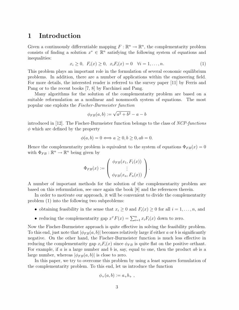
1 Introduction

Given a continuously differentiable mapping F : Rn → Rn, the complementarity problemconsists of finding a solution x∗ ∈ Rn satisfying the following system of equations andinequalities:

xi ≥ 0, Fi(x) ≥ 0, xiFi(x) = 0 ∀i = 1, . . . , n. (1)

This problem plays an important role in the formulation of several economic equilibriumproblems. In addition, there are a number of applications within the engineering field.For more details, the interested reader is referred to the survey paper [11] by Ferris andPang or to the recent books [7, 8] by Facchinei and Pang.

Many algorithms for the solution of the complementarity problem are based on asuitable reformulation as a nonlinear and nonsmooth system of equations. The mostpopular one exploits the Fischer-Burmeister function

φFB(a, b) :=√a2 + b2 − a− b

introduced in [12]. The Fischer-Burmeister function belongs to the class of NCP-functionsφ which are defined by the property

φ(a, b) = 0⇐⇒ a ≥ 0, b ≥ 0, ab = 0.

Hence the complementarity problem is equivalent to the system of equations ΦFB(x) = 0with ΦFB : Rn → Rn being given by

ΦFB(x) :=

φFB(x1, F1(x))...

φFB(xn, Fn(x))

.

A number of important methods for the solution of the complementarity problem arebased on this reformulation, see once again the book [8] and the references therein.

In order to motivate our approach, it will be convenient to divide the complementarityproblem (1) into the following two subproblems:

• obtaining feasibility in the sense that xi ≥ 0 and Fi(x) ≥ 0 for all i = 1, . . . , n, and

• reducing the complementarity gap xTF (x) =∑n

i=1 xiFi(x) down to zero.

Now the Fischer-Burmeister approach is quite effective in solving the feasibility problem.To this end, just note that |φFB(a, b)| becomes relatively large if either a or b is significantlynegative. On the other hand, the Fischer-Burmeister function is much less effective inreducing the complementarity gap xiFi(x) since φFB is quite flat on the positive orthant.For example, if a is a large number and b is, say, equal to one, then the product ab is alarge number, whereas |φFB(a, b)| is close to zero.

In this paper, we try to overcome this problem by using a least squares formulation ofthe complementarity problem. To this end, let us introduce the function

φ+(a, b) := a+b+ ,

3

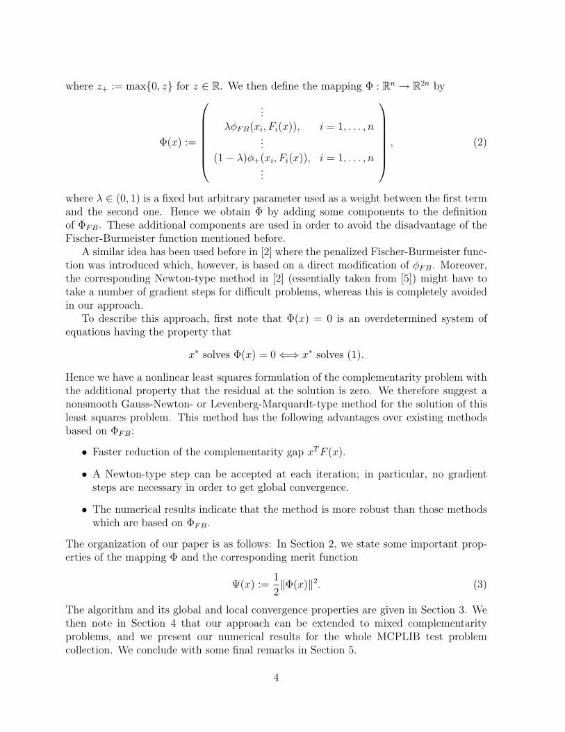
where z+ := max{0, z} for z ∈ R. We then define the mapping Φ : Rn → R2n by

Φ(x) :=

...λφFB(xi, Fi(x)), i = 1, . . . , n

...(1− λ)φ+(xi, Fi(x)), i = 1, . . . , n

...

, (2)

where λ ∈ (0, 1) is a fixed but arbitrary parameter used as a weight between the first termand the second one. Hence we obtain Φ by adding some components to the definitionof ΦFB. These additional components are used in order to avoid the disadvantage of theFischer-Burmeister function mentioned before.

A similar idea has been used before in [2] where the penalized Fischer-Burmeister func-tion was introduced which, however, is based on a direct modification of φFB. Moreover,the corresponding Newton-type method in [2] (essentially taken from [5]) might have totake a number of gradient steps for difficult problems, whereas this is completely avoidedin our approach.

To describe this approach, first note that Φ(x) = 0 is an overdetermined system ofequations having the property that

x∗ solves Φ(x) = 0⇐⇒ x∗ solves (1).

Hence we have a nonlinear least squares formulation of the complementarity problem withthe additional property that the residual at the solution is zero. We therefore suggest anonsmooth Gauss-Newton- or Levenberg-Marquardt-type method for the solution of thisleast squares problem. This method has the following advantages over existing methodsbased on ΦFB:

• Faster reduction of the complementarity gap xTF (x).

• A Newton-type step can be accepted at each iteration; in particular, no gradientsteps are necessary in order to get global convergence.

• The numerical results indicate that the method is more robust than those methodswhich are based on ΦFB.

The organization of our paper is as follows: In Section 2, we state some important prop-erties of the mapping Φ and the corresponding merit function

Ψ(x) :=1

2‖Φ(x)‖2. (3)

The algorithm and its global and local convergence properties are given in Section 3. Wethen note in Section 4 that our approach can be extended to mixed complementarityproblems, and we present our numerical results for the whole MCPLIB test problemcollection. We conclude with some final remarks in Section 5.

4

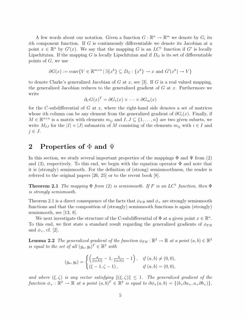
A few words about our notation. Given a function G : Rn → Rm we denote by Gi itsith component function. If G is continuously differentiable we denote its Jacobian at apoint x ∈ Rn by G′(x). We say that the mapping G is an LC1 function if G′ is locallyLipschitzian. If the mapping G is locally Lipschitzian and if DG is its set of differentiablepoints of G, we use

∂G(x) := conv{V ∈ Rm×n | ∃{xk} ⊆ DG : {xk} → x and G′(xk)→ V }

to denote Clarke’s generalized Jacobian of G at x, see [3]. If G is a real valued mapping,the generalized Jacobian reduces to the generalized gradient of G at x. Furthermore wewrite

∂CG(x)T = ∂G1(x)× · · · × ∂Gm(x)

for the C-subdifferential of G at x, where the right-hand side denotes a set of matriceswhose ith column can be any element from the generalized gradient of ∂Gi(x). Finally, ifM ∈ Rn×n is a matrix with elements mij and I, J ⊆ {1, . . . , n} are two given subsets, wewrite MIJ for the |I| × |J | submatrix of M consisting of the elements mij with i ∈ I andj ∈ J .

2 Properties of Φ and Ψ

In this section, we study several important properties of the mappings Φ and Ψ from (2)and (3), respectively. To this end, we begin with the equation operator Φ and note thatit is (strongly) semismooth. For the definition of (strong) semismoothness, the reader isreferred to the original papers [26, 25] or to the recent book [8].

Theorem 2.1 The mapping Φ from (2) is semismooth. If F is an LC1 function, then Φis strongly semismooth.

Theorem 2.1 is a direct consequence of the facts that φFB and φ+ are strongly semismoothfunctions and that the composition of (strongly) semismooth functions is again (strongly)semismooth, see [13, 8].

We next investigate the structure of the C-subdifferential of Φ at a given point x ∈ Rn.To this end, we first state a standard result regarding the generalized gradients of φFBand φ+, cf. [2].

Lemma 2.2 The generalized gradient of the function φFB : R2 → R at a point (a, b) ∈ R2

is equal to the set of all (ga, gb)T ∈ R2 with

(ga, gb) =

{(a

‖(a,b)‖ − 1, b‖(a,b)‖ − 1

), if (a, b) 6= (0, 0),

(ξ − 1, ζ − 1) , if (a, b) = (0, 0),

and where (ξ, ζ) is any vector satisfying ‖(ξ, ζ)‖ ≤ 1. The generalized gradient of thefunction φ+ : R2 → R at a point (a, b)T ∈ R2 is equal to ∂φ+(a, b) = {(b+∂a+, a+∂b+)},

5

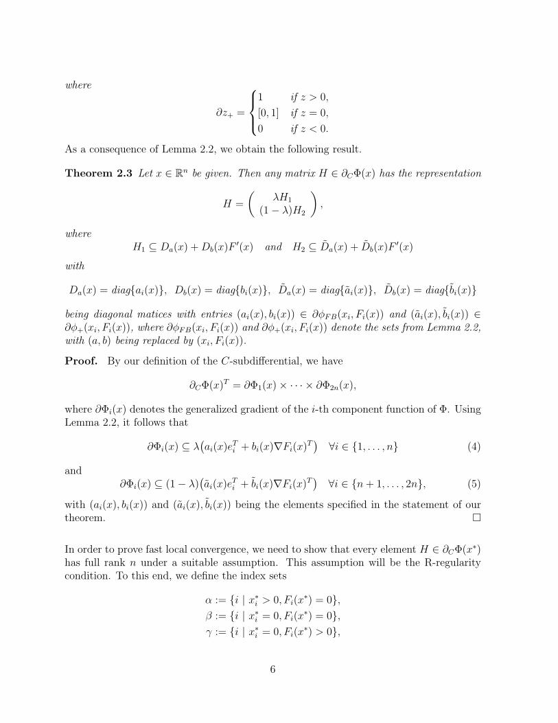
where

∂z+ =

1 if z > 0,

[0, 1] if z = 0,

0 if z < 0.

As a consequence of Lemma 2.2, we obtain the following result.

Theorem 2.3 Let x ∈ Rn be given. Then any matrix H ∈ ∂CΦ(x) has the representation

H =

(λH1

(1− λ)H2

),

whereH1 ⊆ Da(x) +Db(x)F

′(x) and H2 ⊆ Da(x) + Db(x)F′(x)

with

Da(x) = diag{ai(x)}, Db(x) = diag{bi(x)}, Da(x) = diag{ai(x)}, Db(x) = diag{bi(x)}

being diagonal matices with entries (ai(x), bi(x)) ∈ ∂φFB(xi, Fi(x)) and (ai(x), bi(x)) ∈∂φ+(xi, Fi(x)), where ∂φFB(xi, Fi(x)) and ∂φ+(xi, Fi(x)) denote the sets from Lemma 2.2,with (a, b) being replaced by (xi, Fi(x)).

Proof. By our definition of the C-subdifferential, we have

∂CΦ(x)T = ∂Φ1(x)× · · · × ∂Φ2n(x),

where ∂Φi(x) denotes the generalized gradient of the i-th component function of Φ. UsingLemma 2.2, it follows that

∂Φi(x) ⊆ λ(ai(x)e

Ti + bi(x)∇Fi(x)T

)∀i ∈ {1, . . . , n} (4)

and∂Φi(x) ⊆ (1− λ)

(ai(x)e

Ti + bi(x)∇Fi(x)T

)∀i ∈ {n+ 1, . . . , 2n}, (5)

with (ai(x), bi(x)) and (ai(x), bi(x)) being the elements specified in the statement of ourtheorem. �

In order to prove fast local convergence, we need to show that every element H ∈ ∂CΦ(x∗)has full rank n under a suitable assumption. This assumption will be the R-regularitycondition. To this end, we define the index sets

α := {i | x∗i > 0, Fi(x∗) = 0},

β := {i | x∗i = 0, Fi(x∗) = 0},

γ := {i | x∗i = 0, Fi(x∗) > 0},

6

and recall that a solution x∗ of the complementarity problem is called R-regular if thesubmatrix F ′(x∗)αα is nonsingular and the Schur complement

F ′(x∗)ββ − F ′(x∗)βαF′(x∗)−1

ααF′(x∗)αβ

is a P -matrix (see [27, 4]). Then we have the following result.

Theorem 2.4 Let x∗ ∈ Rn be an R-regular solution of the complementarity problem.Then all elements from the C-subdifferential ∂ΦC(x∗) have full rank.

Proof. Let H ∈ ∂CΦ(x∗). In view of Theorem 2.3, we then have

H =

(λH1

(1− λ)H2

),

where H1 is an element from ∂CΦFB(x∗). It now follows from [9, 5] that each elementH1 ∈ ∂CφFB(x∗) is nonsingular under the assumed R-regularity condition. Therefore wehave rank(H) = n, i.e., H has full rank. �

We next state a consequence of Theorem 2.4 that will play an important role in ourconvergence analysis.

Lemma 2.5 Let x∗ ∈ Rn be an R-regular solution of the complementarity problem. Thenthere exist constants ε > 0 and c > 0 such that

‖(HTH)−1‖ ≤ c

for all H ∈ ∂CΦ(x) and all x ∈ Rn with ‖x− x∗‖ ≤ ε.

Proof. The proof is similar to one given in [25] in a slightly different situation. Ifthe claim is not true, there exists a sequence {xk} converging to x∗ and a correspondingsequence of matrices {Hk} with Hk ∈ ∂CΦ(xk) for all k ∈ N such that either HT

k Hk issingular or ‖(HT

k Hk)−1‖ → ∞ on a subsequence. Noting that HT

k Hk is symmetric posi-tive semidefinite, we have ‖(HT

k Hk)−1‖ = 1

λmin(HTk Hk)

in the nonsingular case. Hence the

condition ‖(HTk Hk)

−1‖ → ∞ is equivalent to λmin(HTk Hk) → 0. Since {xk} → x∗ and

the mapping x 7→ ∂CΦ(x) is upper semicontinuous, it follows that the sequence {Hk} isbounded and therefore has a convergent subsequence. Let H∗ be a limiting element ofsuch a subsequence. It then follows that either HT

∗ H∗ is singular or λmin(HT∗ H∗) = 0 (note

that the mapping A 7→ λmin(ATA) is continuous), i.e., H∗ is not of full rank. On the other

hand, exploiting the fact that the mapping x 7→ ∂CΦ(x) is closed, we have H∗ ∈ ∂CΦ(x∗),so that H∗ is of full rank by Theorem 2.4. This contradiction completes the proof. �

We next investigate the properties of the merit function Ψ from (3). To this end, it willbe useful to rewrite this function as

Ψ(x) =1

2‖Φ(x)‖2 =

n∑i=1

ψ(xi, Fi(x))

7

with ψ : R2 → R being defined by

ψ(a, b) :=1

2λ2φ2

FB(a, b) +1

2(1− λ)2a2

+b2+. (6)

The following properties of ψ are crucial in order to state several interesting results for thecorresponding merit function Ψ. Basically, the next result says that ψ shares all the niceproperties of the merit function corresponding to the Fischer-Burmeister function φFB.

Lemma 2.6 The mapping ψ : R2 → R from (6) has the following properties:

(a) ψ is continuously differentiable on R2.

(b) ψ(a, b) ≥ 0 for all a, b ∈ R2.

(c) ψ(a, b) = 0⇐⇒ a ≥ 0, b ≥ 0 and ab = 0.

(d) ∂ψ∂a

(a, b)∂ψ∂b

(a, b) ≥ 0 for all a, b ∈ R2.

(e) ψ(a, b) = 0⇐⇒ ∇ψ(a, b) = 0⇐⇒ ∂ψ∂a

(a, b) = 0⇐⇒ ∂ψ∂b

(a, b) = 0.

Proof. Statements (a) and (b) follow directly from the definition of ψ together with thefact that φ2

FB is known to be continuously differentiable on R2, see [14, 9]. Property (c)follows from the fact that φFB is an NCP-function. Hence it remains to show statements(d) and (e). Since both statements obviously hold for (a, b) = (0, 0), we can assumewithout loss of generality that (a, b) 6= (0, 0) for the rest of this proof.

In order to verify part (d), first note that we have

∂ψ

∂a(a, b)

∂ψ

∂b(a, b)

= λ4φ2FB(a, b)

( a√a2 + b2

− 1)( b√

a2 + b2− 1

)+ (1− λ)4a3

+b3+ + λ2(1− λ)2t(a, b)

with t : R2 → R being defined by

t(a, b) := φFB(a, b)a+b+

[( a√a2 + b2

− 1)a+ +

( b√a2 + b2

− 1)b+

].

It is easy to see that it suffices to prove that t(a, b) ≥ 0. Now, we obviously have t(a, b) ≥ 0if a ≥ 0 and b ≥ 0. On the other hand, in all other cases, we have t(a, b) = 0, so thatstatement (d) follows.

To prove part (e), we first recall that we have (a, b) 6= (0, 0). Furthermore, taking intoaccount the fact that an unconstrained minimum of a continuously differentiable functionis always a stationary point of this function and using the symmetry of the function ψwith respect to its arguments a and b, we only have to verify the implication

∂ψ

∂a(a, b) = 0 =⇒ ψ(a, b) = 0.

8

To this end, we first note that

∂ψ

∂a(a, b) = λ2φFB(a, b)

( a√a2 + b2

− 1)

+ (1− λ)2a+b2+.

Using ∂ψ∂a

(a, b) = 0, let us consider two cases: If a ≤ 0 or b ≤ 0, we have a+b2+ = 0 and

therefore

0 =∂ψ

∂a(a, b) = λ2φFB(a, b)

( a√a2 + b2

− 1).

This implies

φFB(a, b) = 0 ora√

a2 + b2− 1 = 0

which, in turn, is equivalent to

φFB(a, b) = 0 or(a > 0 and b = 0

).

Hence we immediately have ψ(a, b) = 0.Now consider the second case where a > 0 and b > 0. Then we get φFB(a, b) ≤ 0 and

thereforeφFB(a, b)

( a√a2 + b2

− 1)≥ 0.

Consequently, we obtain from

0 =∂ψ

∂a(a, b) = λ2φFB(a, b)

( a√a2 + b2

− 1)

+ (1− λ)2a+b2+

that both sums must be equal to zero. In particular, we therefore have

0 = λ2φFB(a, b)( a√

a2 + b2− 1

).

Hence we can argue as in the first case and see that ψ(a, b) = 0. �

Using Lemma 2.6, we obtain the following properties of the merit function Ψ in essentiallythe same way as they can be obtained for some other merit functions, see [5, 9, 14] aswell as [19] regarding the compact level sets for monotone problems. We therefore donot state the corresponding proofs here. As for the definition of a P0-matrix occuringin statement (b), the reader is referred to [4]. For the notion of a (uniform) P -function,see [22]. Furthermore, recall that the complementarity problem (1) is said to be strictlyfeasible if there is a vector x ∈ Rn such that x > 0 and F (x) > 0.

Theorem 2.7 The merit function Ψ from (3) has the following properties:

(a) Ψ is continuously differentiable with ∇Ψ(x) = HTΦ(x), where H ∈ ∂CΦ(x) can bechosen arbitrarily.

9

(b) If x∗ is a stationary point of Ψ and F ′(x∗) is a P0-matrix, then x∗ is a solution ofthe complementarity problem.

(c) If F is either a uniform P -function or if F is monotone and the complementarityproblem (1) is strictly feasible, then the level sets

L(c) :={x ∈ Rn

∣∣ Ψ(x) ≤ c}

are compact for all c ∈ R.

We close this section by noting that there are some other merit functions which sharethe properties from Theorem 2.7, see [19, 2]. However, we are not aware of any meritfunction having stronger properties, while there are a couple of merit functions (includingthe Fischer-Burmeister merit function) which satisfy only some weaker conditions, see[21, 20, 14].

3 Algorithm and Convergence

We first state our algorithm for the solution of the complementarity problem (1). It is aLevenberg-Marquardt-type method applied to the nonlinear least squares problem

min Ψ(x) =1

2‖Φ(x)‖2,

where, of course, Φ and Ψ denote the mappings from (2) and (3), respectively.

Algorithm 3.1 (Semismooth Levenberg-Marquardt Method)

(S.0) Let β ∈ (0, 1), σ ∈ (0, 12) and ε ≥ 0. Choose any x0 ∈ Rn. Set k := 0.

(S.1) If ‖∇Ψ(xk)‖ ≤ ε: STOP.

(S.2) Choose Hk ∈ ∂CΦ(xk), λk > 0 and find a solution dk ∈ Rn of(HTk Hk + λkI

)d = −∇Ψ(xk). (7)

(S.3) Compute tk = max{βl | l = 0, 1, 2, . . . } such that

Ψ(xk + tkdk) ≤ Ψ(xk) + σtk∇Ψ(xk)Tdk. (8)

Set xk+1 = xk + tkdk, k ← k + 1, and go to (S.1).

We now investigate the convergence properties of our algorithm. To this end, we assumethat the termination parameter ε is equal to zero and that Algorithm 3.1 generates aninfinite sequence. We further note that Algorithm 3.1 is well defined since λk > 0 andsince one can easily see that the search direction dk is always a descent direction for themerit function Ψ.

10

We first state a global convergence result. For the sake of simplicity, we assume thatλk is given by

λk := ‖∇Ψ(xk)‖, (9)

although several other choices of λk yield the same result including the more realisticchoice

λk := min{c1, c2‖∇Ψ(xk)‖}

for certain constants c1, c2 > 0. Note that these choices are consistent with the require-ments for local superlinear/quadratic convergence in Theorem 3.3 below.

Theorem 3.2 Algorithm 3.1 is well defined for an arbitrary complementarity problem.Furthermore, every accumulation point of a sequence {xk} generated by Algorithm 3.1 isa stationary point of Ψ.

Proof. As noticed above the algorithm is well defined. Let x∗ be any accumulationpoint of the sequence {xk} and {xk}K a subsequence converging to x∗. Suppose that∇Ψ(x∗) 6= 0. Due to the monotone decrease of the sequence {Ψ(xk)} and the fact that{Ψ(xk)}K converges to Ψ(x∗), it follows that the entire sequence {Ψ(xk)} converges toΨ(x∗). In particular, we therefore have

Ψ(xk+1)−Ψ(xk)→ 0.

On the other hand, we obtain

Ψ(xk+1)−Ψ(xk) ≤ σtk∇Ψ(xk)Tdk ≤ 0

by Step (S.3) in Algorithm 3.1 and the descent property of the search direction dk. Hencewe have

{tk∇Ψ(xk)Tdk}K → 0. (10)

Using the definition of the Levenberg-Marquardt direction gives

tk∇Ψ(xk)Tdk = −tk∇Ψ(xk)T (HTk Hk + λkI)

−1∇Ψ(xk). (11)

Since {xk}K → x∗, we get from the upper semicontinuity of the C-subdifferential that thesequence {Hk}K is bounded. Without loss of generality, we therefore have {Hk}K → H∗for some matrix H∗ ∈ ∂CΦ(x∗). Since ∇Ψ is continuous, we also obtain {∇Ψ(xk)}K →∇Ψ(x∗) and therefore {λk}K → λ∗ with λ∗ := ‖∇Ψ(x∗)‖ > 0, cf. (9). Using thesearguments, it follows that the matrices

HTk Hk + λkI

converge to the symmetric positive definite matrix HT∗ H∗ + λ∗I on the subset K ⊆ N.

From (10), (11) we therefore obtain

{tk}K → 0.

11

Now, for each k ∈ N, let lk ∈ N be the uniquely defined exponent such that tk = βlk .It follows that the Armijo-rule in Step (S.3) is not satisfied for βlk−1 for sufficiently largek ∈ K. Hence, we have

Ψ(xk + βlk−1dk)−Ψ(xk)

βlk−1> σ∇Ψ(xk)Tdk (12)

for all these k ∈ K. From the Levenberg-Marquardt equation we obtain {dk}K → d∗, withd∗ being the solution of the linear system(

HT∗ H∗ + λ∗I

)d = −∇Ψ(x∗).

Taking into account that {dk}K → d∗, {xk}K → x∗ and {tk}K → 0, we obtain from (12)that

∇Ψ(x∗)Td∗ ≥ σ∇Ψ(x∗)Td∗.

Hence ∇Ψ(x∗)Td∗ ≥ 0, since σ ∈ (0, 12). On the other hand, we have

∇Ψ(x∗)Td∗ = −∇Ψ(x∗)T (HT∗ H∗ + λ∗I)

−1∇Ψ(x∗) < 0.

This contradiction shows that x∗ is a stationary point of Ψ. �

Recall that Theorem 2.7 (b) gives a relatively mild condition for a stationary point ofΨ to be a solution of the complementarity problem (1). Furthermore, the existence of astationary point follows, e.g., under the assumptions of Theorem 2.7 (c).

We next investigate the rate of convergence of Algorithm 3.1. Obviously, this rate ofconvergence depends on the choice of the Levenberg-Marquardt parameter λk.

Theorem 3.3 Let {xk} be a sequence generated by Algorithm 3.1. Assume that x∗ is anaccumulation point of {xk} such that x∗ is an R-regular solution of the complementarityproblem (1). Then the following statements hold:

(a) The entire sequence {xk} converges to x∗ if {λk} is bounded.

(b) The full stepsize tk = 1 is always accepted for k sufficiently large so that xk+1 =xk + dk provided that λk → 0.

(c) The rate of convergence is Q-superlinear if λk → 0.

(d) The rate of convergence is Q-quadratic if λk = O(‖∇Ψ(xk)‖) and, in addition, F isan LC1-function.

Proof. (a) To establish that the entire sequence {xk} converges to x∗, we first note thatan R-regular solution is an isolated solution of the complementarity problem, see [27].Since Algorithm 3.1 generates a decreasing sequence {Ψ(xk)} and x∗ is a solution of thecomplementarity problem, it follows that the entire sequnce {Ψ(xk)} converges to zero.

12

Hence every accumulation point of the sequence {xk} is a solution of (1). Consequently,x∗ is an isolated accumulation point of the sequence {xk}.

Now let {xk}K denote any subsequence converging to x∗, and note that x∗ is a station-ary point of Ψ. For all k ∈ N, we have

‖xk+1 − xk‖ = tk‖dk‖ ≤ ‖dk‖ ≤ ‖(HTk Hk + λkI)

−1‖ ‖∇Ψ(x)‖.

From {∇Ψ(xk)}K → 0, Lemma 2.5 and the assumed boundedness of {λk}, we immediatelyobtain {‖xk+1 − xk‖}K → 0. Hence statement (a) follows from [23, Lemma 4.10].

(b), (c) First we prove that

‖xk + dk − x∗‖ = o(‖xk − x∗‖) (13)

for all k ∈ N sufficiently large. In view of part (a), we know that the entire sequence {xk}converges to the R-regular solution x∗. Hence it follows from Lemma 2.5 that there is aconstant c > 0 such that

‖(HTk Hk + λkI)

−1‖ ≤ c ∀k ∈ N.

Furthermore, the sequence {Hk} is bounded. We can therefore assume without loss ofgenerality that we also have

‖HTk ‖ ≤ c ∀k ∈ N.

Using Theorem 2.7 (a) and Φ(x∗) = 0, we then obtain for all k ∈ N sufficiently large that

‖xk + dk − x∗‖ = ‖xk − (HTk Hk + λkI)

−1∇Ψ(xk)− x∗‖≤ ‖(HT

k Hk + λkI)−1‖ ‖∇Ψ(xk)− (HT

k Hk + λkI)(xk − x∗)‖

≤ c ‖HTk Φ(xk)−HT

k Hk(xk − x∗)− λk(xk − x∗)‖

= c ‖HTk

(Φ(xk)− Φ(x∗)−Hk(x

k − x∗))− λk(xk − x∗)‖

≤ c(‖HT

k ‖ ‖(Φ(xk)− Φ(x∗)−Hk(xk − x∗)‖+ λk‖xk − x∗‖

)≤ c

(c‖Φ(xk)− Φ(x∗)−Hk(x

k − x∗)‖+ λk‖xk − x∗‖).

Since Φ is semismooth by Theorem 2.1, it follows that

‖Φ(xk)− Φ(x∗)−Hk(xk − x∗)‖ = o(‖xk − x∗‖)

see [26, 25, 8]. Using the fact that λk → 0 by assumption, we therefore obtain (13).In order to prove that the full step is eventually accepted, we next show that

limk→∞

Ψ(xk + dk)

Ψ(xk)= 0 (14)

and

1 + σ∇Ψ(xk)Tdk

Ψ(xk)≥ 1− 2σ > 0 (15)

13

holds for all sufficiently large k ∈ N. Since Ψ(xk) 6= 0 for all k ∈ N, we get from Theorem2.7 (a) that

∇Ψ(xk)Tdk

Ψ(xk)= −(HT

k Φ(xk))T (HTk Hk + λkI)

−1HTk Φ(xk)

12‖Φ(xk)‖

≥ −Φ(xk)THk(HTk Hk)

−1HTk Φ(xk)

12‖Φ(xk)‖

≥ −Φ(xk)TΦ(xk)12‖Φ(xk)‖

= −2,

(16)

where the second inequality in (16) follows from

dTAd ≤ λmax(A)‖d‖2 ∀d ∈ Rn

and all symmetric matrices A ∈ Rn×n by noting that the maximal eigenvalue of thesymmetric matrix A := Hk(H

Tk Hk)

−1HTk is equal to one. The inequality (15) now follows

from (16).To verify (14), we only have to show that

limk→∞

‖Φ(xk + dk)‖‖Φ(xk)‖

= 0 (17)

holds. To this end, we first note that there exists a constant α > 0 such that

‖Φ(xk)‖ ≥ α‖xk − x∗‖ (18)

for all k ∈ N sufficiently large. This follows from the simple observation that ‖Φ(x)‖ ≥λ‖ΦFB(x)‖ together with the fact that all elements V ∈ ∂ΦFB(x∗) are nonsingular underthe R-regularity condition as well as [24, Proposition 3]. Using (18) and (13), we obtain

‖Φ(xk + dk)‖‖Φ(xk)‖

≤ ‖Φ(xk + dk)‖α‖xk − x∗‖

=‖Φ(xk + dk)− Φ(x∗)‖

α‖xk − x∗‖

≤ L‖xk + dk − x∗‖α‖xk − x∗‖

→ 0,

where L > 0 denotes the local Lipschitz constant of Φ. Hence (17) holds.Using (14) and (15), we see that the condition

Ψ(xk + dk) ≤ Ψ(xk) + σ∇Ψ(xk)Tdk

14

or, equivalently,Ψ(xk + dk)

Ψ(xk)≤ 1 + σ

∇Ψ(xk)Tdk

Ψ(xk)

is satisfied for all k ∈ N sufficiently large. Hence the stepsize tk = 1 is eventually acceptedin the line search criterion, and we have xk+1 = xk + dk for all k ∈ N large enough. HenceQ-superlinear convergence of {xk} to x∗ follows from (13).

(d) The proof is essentially the same as for the local superlinear convergence. To thisend, we only note that F being an LC1 function implies that Φ is stronlgy semismoothby Theorem 2.1, and that the relation

‖Φ(xk)− Φ(x∗)−Hk(xk − x∗)‖ = O(‖xk − x∗‖2).

holds for strongly semismooth functions, see [26, 25, 8]. �

Note that the previous proof is similar to one given in [16]. We stress, however, that [16]considers a Levenberg-Marquardt-type method for a square system of equations, whereaswe are dealing with a nonsquare (overdetermined) system.

4 Extension to Mixed Complementarity Problems and

Computational Results

4.1 Extension to Mixed Complementarity Problems

In this subsection, we would like to point out that the approach presented for the stan-dard complementarity problem (1) can actually be extended to the more general mixedcomplementarity problem. We only sketch the idea here and do not state any formalresults.

In order to introduce the mixed complementarity problem, it is quite convenient toconsider the variational inequality problem first. For a given function F : Rn → Rn and anonempty, closed and convex set X ⊆ Rn, this variational inequality problem consists infinding a point x∗ ∈ X such that

F (x∗)T (x− x∗) ≥ 0 ∀x ∈ X.

It is well-known and easy to see that this variational inequality problem is equivalentto the complementarity problem (1) when X is equal to the nonnegative orthant, i.e.,if X = [0,∞). On the other hand, if X = [l, u] is a general box with lower boundsl = (l1, . . . , ln)

T and upper bounds u = (u1, . . . , un)T satisfying −∞ ≤ li < ui ≤ +∞ for

all i ∈ {1, . . . , n}, we obtain the mixed complementarity problem.

15

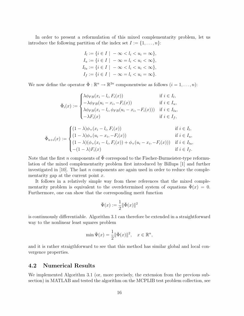
In order to present a reformulation of this mixed complementarity problem, let usintroduce the following partition of the index set I := {1, . . . , n}:

Il := {i ∈ I | −∞ < li < ui =∞},Iu := {i ∈ I | −∞ = li < ui <∞},Ilu := {i ∈ I | −∞ < li < ui <∞},If := {i ∈ I | −∞ = li < ui =∞}.

We now define the operator Φ : Rn → R2n componentwise as follows (i = 1, . . . , n):

Φi(x) :=

λφFB(xi − li, Fi(x)) if i ∈ Il,−λφFB(ui − xi,−Fi(x)) if i ∈ Iu,λφFB(xi − li, φFB(ui − xi,−Fi(x))) if i ∈ Ilu,−λFi(x) if i ∈ If ,

Φn+i(x) :=

(1− λ)φ+(xi − li, Fi(x)) if i ∈ Il,(1− λ)φ+(ui − xi,−Fi(x)) if i ∈ Iu,(1− λ)(φ+(xi − li, Fi(x)) + φ+(ui − xi,−Fi(x))) if i ∈ Ilu,−(1− λ)Fi(x) if i ∈ If .

Note that the first n components of Φ correspond to the Fischer-Burmeister-type reformu-lation of the mixed complementarity problem first introduced by Billups [1] and furtherinvestigated in [10]. The last n components are again used in order to reduce the comple-mentarity gap at the current point x.

It follows in a relatively simple way from these references that the mixed comple-mentarity problem is equivalent to the overdetermined system of equations Φ(x) = 0.Furthermore, one can show that the corresponding merit function

Ψ(x) :=1

2‖Φ(x)‖2

is continuously differentiable. Algorithm 3.1 can therefore be extended in a straightforwardway to the nonlinear least squares problem

min Ψ(x) =1

2‖Φ(x)‖2, x ∈ Rn,

and it is rather straigthforward to see that this method has similar global and local con-vergence properties.

4.2 Numerical Results

We implemented Algorithm 3.1 (or, more precisely, the extension from the previous sub-section) in MATLAB and tested the algorithm on the MCPLIB test problem collection, see

16

[6] (note that we use a newer version of this test problem collection). The implementationcorresponds exactly to the statement of Algorithm 3.1 except that we use a nonmonotoneline search as introduced by Grippo, Lampariello and Lucidi [15]. To be more precise, weuse the standard (monotone) Armijo rule during the first five iterations and then switchto the nonmonotone line search where the maximum of the function values Ψ(xk) is takenover the last ten iterations, see [15] for further details.

We terminate the iteration if one of the following conditions are satisfied

‖Φ(xk)‖ ≤ 10−11 or ‖∇Ψ(xk)‖ ≤ 10−6 or k > 300,

and we choose λk := 0 for all k ∈ N so that our Levenberg-Marquardt method becomesa Gauss-Newton-type algorithm. The other parameters used in our implementation areλ = 0.1, β = 0.55, σ = 10−4. The procedure for calculating an element Hk ∈ ∂CΦ(xk) issimilar to one given in [5] for the Fischer-Burmeister equation operator.

Our numerical results are summarized in Table 1 for small dimensional problems andin Table 2 for large dimensional ones. In these tables the first column gives the name ofthe problem; Dim is the number of the variables in the problem; Ψ(x0) gives the value ofthe merit function at the starting point; Nit denotes the number of iterations; Ψ(xf ) and‖∇Ψ(xf )‖ denote the values of Ψ(x) and ‖∇Ψ(x)‖ at the final iterate x = xf . Note thatNit is equal to the number of linear subproblems solved.

Table 1: Numerical results for MCPLIB test problems

Problem Dim Ψ(x0) Nit Ψ(xf ) ‖∇Ψ(xf )‖badfree 5 4.600000e–01 2 3.802055e–13 1.120124e–06bertsekas 15 3.936098e–03 38 2.754293e–16 1.468242e–07billups 1 3.451182e–05 30 2.153258e–12 7.538314e–06choi 13 7.709002e–03 5 2.649619e–16 1.278982e–09colvdual 20 5.488000e+01 19 8.785822e–12 1.096167e–05colvnlp 15 6.207596e+01 6 4.033072e–15 2.298057e–07cycle 1 5.173835e+01 5 3.703547e–21 7.746281e–10degen 2 1.000000e–01 5 6.295417e–17 1.122182e–09duopoly 63 2.132546e+02 — — —ehl-k40 41 1.042178e+04 32 2.335817e–14 6.724183e–06ehl-k60 61 3.797546e+04 43 4.583751e–14 1.039908e–05ehl-k80 81 9.363011e+04 50 1.115490e–12 3.133144e–03ehl-kost 101 1.878951e+05 113 1.021911e–12 5.417297e–03electric 158 2.609736e+08 33 8.195661e–13 2.421314e–06explcp 16 3.200000e–01 19 5.723100e–16 3.383225e–09forcebsm 184 3.944244e+03 239 3.095727e–12 2.489442e–07forcedsa 186 3.948661e+03 25 2.971468e–16 2.437821e–09freebert 15 1.509811e+04 10 6.212865e–14 2.194618e–06gafni 5 1.300358e+03 10 6.470323e–13 3.651867e–05

17

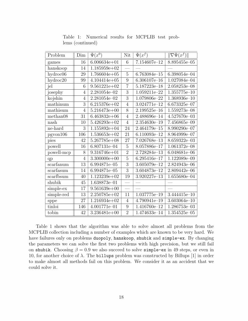
Table 1: Numerical results for MCPLIB test prob-lems (continued)

Problem Dim Ψ(x0) Nit Ψ(xf ) ‖∇Ψ(xf )‖games 16 6.006634e+01 6 7.154607e–12 8.895455e–05hanskoop 14 1.185959e+02 — — —hydroc06 29 1.766604e+05 5 6.763084e–15 6.398054e–04hydroc20 99 4.104414e+05 9 6.306107e–16 1.027084e–04jel 6 9.561221e+02 7 5.187223e–18 2.058253e–08josephy 4 2.281054e–02 3 1.059211e–22 1.355775e–10kojshin 4 2.281054e–02 3 1.079806e–22 1.368936e–10mathinum 3 6.215376e+02 4 3.024771e–12 6.673325e–07mathisum 4 5.216473e+00 8 2.199525e–16 1.559273e–08methan08 31 6.463832e+06 4 2.488696e–14 4.527670e–03nash 10 5.426293e+02 4 2.354630e–19 7.456865e–09ne-hard 3 1.155892e+04 24 2.464179e–15 8.990290e–07pgvon106 106 1.536653e+02 21 6.110093e–12 8.964999e–07pies 42 5.267785e+08 27 7.026768e–13 8.659322e–03powell 16 6.807131e–04 5 8.057886e–17 1.061372e–08powell-mcp 8 9.316746e+01 2 2.728284e–13 6.048681e–06qp 4 3.300000e+00 5 6.295416e–17 1.122089e–09scarfanum 13 6.994871e–05 3 3.605079e–12 2.824943e–06scarfasum 14 6.994871e–05 3 3.604873e–12 2.809442e–06scarfbsum 40 1.123239e+02 19 3.920227e–13 1.655680e–04shubik 45 1.638873e–01 — — —simple-ex 17 9.561639e+00 — — —simple-red 13 2.250785e+02 11 1.037775e–19 3.444415e–10sppe 27 1.216934e+02 4 4.790941e–19 3.603064e–10tinloi 146 4.001771e–01 9 1.416760e–12 1.286753e–03tobin 42 3.236481e+00 2 1.474633e–14 1.354525e–05

Table 1 shows that the algorithm was able to solve almost all problems from theMCPLIB collection including a number of examples which are known to be very hard. Wehave failures only on problems duopoly, hanskoop, shubik and simple-ex. By changingthe parameters we can solve the first two problems with high precision, but we still failon shubik. Choosing β = 0.9 we also succeed to solve simple-ex in 49 steps, or even in10, for another choice of λ. The billups problem was constructed by Billups [1] in orderto make almost all methods fail on this problem. We consider it as an accident that wecould solve it.

18

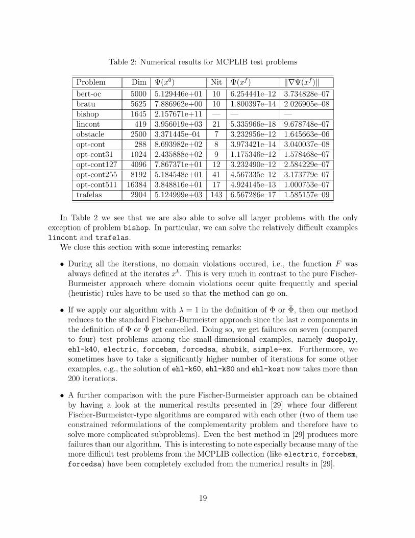
Table 2: Numerical results for MCPLIB test problems

Problem Dim Ψ(x0) Nit Ψ(xf ) ‖∇Ψ(xf )‖bert-oc 5000 5.129446e+01 10 6.254441e–12 3.734828e–07bratu 5625 7.886962e+00 10 1.800397e–14 2.026905e–08bishop 1645 2.157671e+11 — — —lincont 419 3.956019e+03 21 5.335966e–18 9.678748e–07obstacle 2500 3.371445e–04 7 3.232956e–12 1.645663e–06opt-cont 288 8.693982e+02 8 3.973421e–14 3.040037e–08opt-cont31 1024 2.435888e+02 9 1.175346e–12 1.578468e–07opt-cont127 4096 7.867371e+01 12 3.232490e–12 2.584229e–07opt-cont255 8192 5.184548e+01 41 4.567335e–12 3.173779e–07opt-cont511 16384 3.848816e+01 17 4.924145e–13 1.000753e–07trafelas 2904 5.124999e+03 143 6.567286e–17 1.585157e–09

In Table 2 we see that we are also able to solve all larger problems with the onlyexception of problem bishop. In particular, we can solve the relatively difficult exampleslincont and trafelas.

We close this section with some interesting remarks:

• During all the iterations, no domain violations occured, i.e., the function F wasalways defined at the iterates xk. This is very much in contrast to the pure Fischer-Burmeister approach where domain violations occur quite frequently and special(heuristic) rules have to be used so that the method can go on.

• If we apply our algorithm with λ = 1 in the definition of Φ or Φ, then our methodreduces to the standard Fischer-Burmeister approach since the last n components inthe definition of Φ or Φ get cancelled. Doing so, we get failures on seven (comparedto four) test problems among the small-dimensional examples, namely duopoly,ehl-k40, electric, forcebsm, forcedsa, shubik, simple-ex. Furthermore, wesometimes have to take a significantly higher number of iterations for some otherexamples, e.g., the solution of ehl-k60, ehl-k80 and ehl-kost now takes more than200 iterations.

• A further comparison with the pure Fischer-Burmeister approach can be obtainedby having a look at the numerical results presented in [29] where four differentFischer-Burmeister-type algorithms are compared with each other (two of them useconstrained reformulations of the complementarity problem and therefore have tosolve more complicated subproblems). Even the best method in [29] produces morefailures than our algorithm. This is interesting to note especially because many of themore difficult test problems from the MCPLIB collection (like electric, forcebsm,forcedsa) have been completely excluded from the numerical results in [29].

19

Altogether this indicates that our new approach is certainly more robust and sometimesalso more efficient than the underlying Fischer-Burmeister method.

5 Conclusions

We have introduced a new method for the solution of (mixed and nonlinear) complemen-tarity problems. This method uses a nonlinear least squares reformulation of the comple-mentarity problem and applies a Levenberg-Marquardt-type method to this reformulatedproblem. The main idea of our method is to overcome one of the main disadvantages ofthe well-known Fischer-Burmeister method and to take special attention to the reductionof the complementarity gap. The numerical results indicate that the new method is signif-icantly more robust than the corresponding Fischer-Burmeister equation-based algorithm.

While we have illustrated our technique by modifying the equation-based method usingthe Fischer-Burmeister function, it should be clear that our idea can also be used inorder to modify other equation-based methods, see, for example, [28] for a summary ofmany of these equation reformulations. More precisely, assume we have a reformulationof the complementarity problem (1) as a square system of equations ΦA(x) = 0 withΦA : Rn → Rn. Suppose further that ΦB : Rn → Rm is any mapping with the propertythat ΦB(x) = 0 whenever x is a solution of (1). Then it is easy to see that x∗ is a solutionof the complementarity problem (1) if and only if x∗ is a solution of the overdeterminedsystem of equations Φ(x) = 0, where Φ : Rn → Rn+m is now defined by

Φ(x) :=

(ΦA(x)ΦB(x)

).

Assuming that Φ and the corresponding merit function Ψ(x) := 12‖Φ(x)‖2 have similar

properties as those stated in Section 2 for the functions from (2) and (3), we can applythe Levenberg-Marquardt method from Algorithm 3.1 to the least squares problem

min Ψ(x)

in order to solve the complementarity problem (1). The convergence theory from Section3 still holds for this approach. Of course, the crucial part is the definition of the mappingΦB which depends on the properties of the mapping ΦA.

References

[1] S.C. Billups: Algorithms for complementarity problems and generalized equations.Ph.D. thesis, Computer Sciences Department, University of Wisconsin, Madison,1995.

[2] B. Chen, X. Chen and C. Kanzow: A penalized Fischer-Burmeister NCP-function. Mathematical Programming 88, 2000, pp. 211–216.

20

[3] F.H. Clarke: Optimization and Nonsmooth Analysis. John Wiley & Sons, NewYork, NY, 1983 (reprinted by SIAM, Philadelphia, PA, 1990).

[4] R.W. Cottle, J.-S. Pang and R.E. Stone: The Linear Complementarity Prob-lem. Academic Press, San Diego, 1992.

[5] T. De Luca, F. Facchinei and C. Kanzow: A semismooth equation approachto the solution of nonlinear complementarity problems. Mathematical Programming75, 1996, pp. 407–439.

[6] S.P. Dirkse and M.C. Ferris: MCPLIB: A collection of nonlinear mixed com-plementarity problems. Optimization Methods and Software 5, 1995, pp. 319–345.

[7] F. Facchinei and J.S. Pang: Finite-Dimensional Varitional Inequalities and Com-plementarity Problems, Volume I. Springer, New York, NY, 2003.

[8] F. Facchinei and J.S. Pang: Finite-Dimensional Varitional Inequalities and Com-plementarity Problems, Volume II. Springer, New York, NY, 2003.

[9] F. Facchinei and J. Soares: A new merit function for nonlinear complementarityproblems and a related algorithm. SIAM Journal on Optimization 7, 1997, pp. 225–247.

[10] M.C. Ferris, C. Kanzow and T.S. Munson: Feasible descendent algorithms formixed complemetarity problems. Mathematical Programming 86, 1999, pp. 475–497.

[11] M.C. Ferris and J.S. Pang: Engineering and economic applications of comple-mentarity problems. SIAM Review 39, 1997, pp. 669–713.

[12] A. Fischer: A special Newton-type optimization method. Optimization 24, 1992, pp.269–284.

[13] A. Fischer: Solution of monotone complementarity problems with locally Lips-chitzian function. Mathematical Programming 76, 1997, pp. 513–532.

[14] C. Geiger and C. Kanzow: On the resolution of monotone complementarityproblems. Computational Optimization and Applications 5, 1996, pp. 155–173.

[15] L. Grippo, F. Lampariello and S. Lucidi: A nonmonotone line search techniquefor Newton’s method. SIAM Journal on Numerical Analysis 23, 1986, pp. 707–716.

[16] H. Jiang: Global convergence analysis of the generalized Newton and Gauss-Newtonmethods of the Fischer-Burmeister equation for the complementarity problem. Math-ematics of Operations Research 24, 1999, pp. 529–543.

[17] C. Kanzow: An inexact QP-based method for nonlinear complementarity problems.Numerische Mathematik 80, 1998, pp. 557–577.

21

[18] C. Kanzow: Strictly feasible equation-based methods for mixed complementarityproblems. Numerische Mathematik 89, 2001, pp. 135–160.

[19] C. Kanzow, N. Yamashita and M. Fukushima: New NCP-functions and theirproperties. Journal of Optimization Theory and Applications 94, 1997, pp. 115–135.

[20] Z.Q. Luo and P. Tseng: A new class of merit functions for the nonlinear comple-mentarity problem. In M.C. Ferris and J.S. Pang (eds.): Complementarity andVariational Problems: State of the Art. SIAM, Philadelphia, PA, 1997, pp. 204–225.

[21] O.L. Mangasarian and M.V. Solodov: Nonlinear complementarity as uncon-strained and constrained optimization. Mathematical Programming 62, 1993, pp. 277–298.

[22] J. More and W.C. Rheinboldt: On P - and S-functions and related classes ofn-dimensional nonlinear mappings. Linear Algebra and its Applications 6, 1973, pp.45–68.

[23] J. More and D.C. Sorensen: Computing a trust region step. SIAM Journal onScientific and Statistical Computing 4, 1983, pp. 553–572.

[24] J.-S. Pang and L. Qi: Nonsmooth equations: motivation and algorithms. SIAMJournal on Optimization 3, 1993, pp. 443–465.

[25] L. Qi: Convergence analysis of some algorithms for solving nonsmooth equations.Mathematics of Operations Research 18, 1993, pp. 227–244.

[26] L. Qi and J. Sun: A nonsmooth version of Newton’s method. Mathematical Pro-gramming 58, 1993, pp. 353–367.

[27] S.M. Robinson: Strongly regular generalized equations. Mathematics of OperationsResearch 5, 1980, pp. 43–62.

[28] D. Sun and L. Qi: On NCP-functions. Computational Optimization and Applica-tions 13, 1999, pp. 201–230.

[29] M. Ulbrich: Nonmonotone trust-region methods for bound-constrained semismoothequations with applications to nonlinear mixed complementarity problems. SIAM Jour-nal on Optimization 11, 2001, pp. 889–916.

22