ON A NON-LINEAR FORMULATION FOR CURVED TIMOSHENKO BEAM ELEMENTS CONSIDERING LARGE

DISPLACEMENT/ROTATION INCREMENTS

EDUARDO N. DVORKIN

Institute de Materiales y Esfructuras, Facultad de Ingenieria, Universidad de Buenos Aires, Buenos Aires, Argentina

EUGENIO ORATE AND JAVIER OLIVER

E.T.S. Ingenieros de Caminos, Canales y Puertos, Universidad Politkcnica de Catalunya, Barcelona, Spain

SUMMARY

An incremental Total Lagrangian Formulation for curved beam elements that includes the effect of large rotation increments is developed. A complete and symmetric tangent stiffness matrix is obtained and the numerical results show, in general, an improvement over the standard formulation where the assumption of infinitesimal rotation increments is made in the derivation of the tangent stiffness matrix.

1. INTRODUCTION

The development of structural finite elements (beam and shell elements) for non-linear analysis and the development of solution methods for non-linear problems is a very active research field because the non-linear analysis of structures is an engineering application continuously deman- ding more efficient, robust and above all reliable numerical tools.

The elements with C0 continuity, derived from the Ahmad, Irons and Zienkiewicz shell element1 appear to be the most suitable ones and the majority of the latest developments in the field take this element as a starting point (e.g. References 2-8).

In the development of elements for geometrically non-linear analysis, the consideration of large rotations introduces additional difficulties due to the non-vectorial nature of finite rotations.

In this paper we concentrate in the geometrically non-linear formulation for C0 curved beam elements (also isoparametric beam elements or Timoshenko beam elements).

A derivation of the C0 beam element is presented by Bathe in Reference 9, and an extensive derivation of the kinematics of large rotations is presented by Argyris in Reference 10.

In the standard geometrically non-linear formulation for C0 beam elements the tangent stiffness matrix is derived assuming infinitesimal rotation increments (rotation increments line- arization) and the effect of large rotation increments is considered only during the equilibrium iterations, when calculating the stresses.

Different formulations that take into account the effect of finite rotation increments on the resulting stiffness matrices have been presented by Surana ,I1 by S i m ~ , ' ~ Simo and Vu Quoc13 and by Oiiate.14

In this paper, we develop an incremental Total Lagrangian Formulationg for C0 curved beam elements with finite incremental rotations. This formulation,

0029-5981/88/071597-17$08.50 0 1988 by John Wiley & Sons, Ltd.

Received 15 May 1987 Revised 17 November 1987

1598 E. N. DVORKIN, E. ORATE AND J. OLIVER

(a) includes in the linearization of the equations of motion all the terms that can be considered in a tangent formulation, providing therefore a complete tangent stiffness matrix;

(b) leads to symmetric stiffness matrices.

Numerical results show that, in general, the complete tangent stiffness matrix provides a faster convergence during equilibrium iterations than the stiffness matrix obtained with the standard formulation.

2. KINEMATICS O F THE TIMOSHENKO BEAM ELEMENT

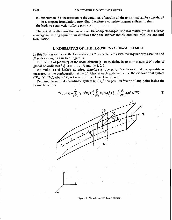
In this Section we review the kinematics of C0 beam elements with rectangular cross section and N nodes along its axis (see Figure 1).

For the initial geometry of the beam element (t =0) we define its axis by means of N nodes of global co-ordinates Ox:; k = 1, . . . , N and i = l ,2,3.

We make use of Bathe's notation, therefore a superscript 0 indicates that the quantity is measured in the configuration at t =0.9 Also, at each node we define the orthonormal system (OV,, OV,, OV,), where OV, is tangent to the element axis (t =O).

Defining the natural co-ordinate system (r, s, t),9 the position vector of any point inside the beam element is

Figure 1. N-node curved beam element

LARGE DISPLACEMENT/ROTATION INCREMENTS 1599

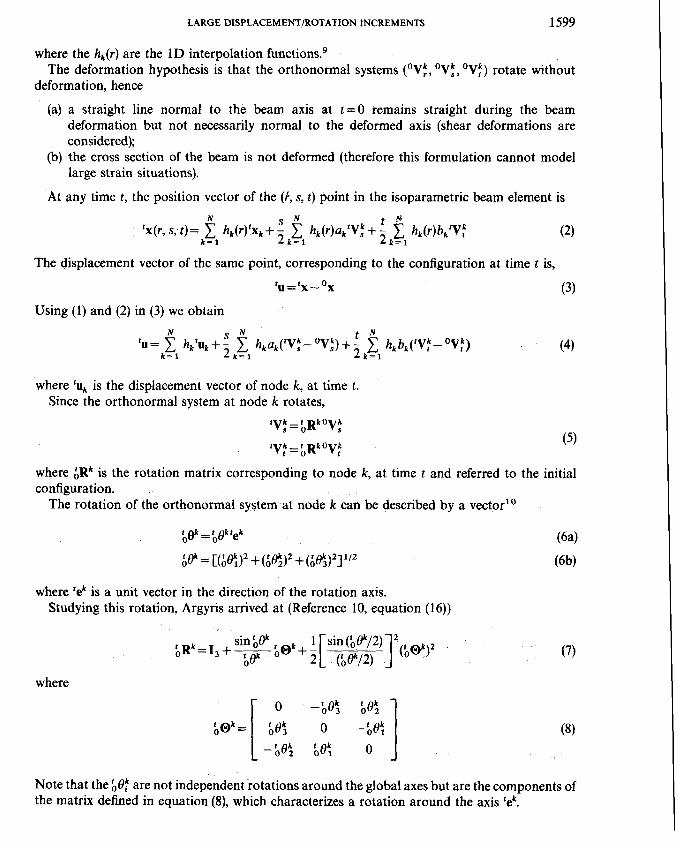
where the hk(r) are the 1D interpolation function^.^ The deformation hypothesis is that the orthonormal systems (OV;, OV;, OV:) rotate without

deformation, hence

(a) a straight line normal to the beam axis at t=O remains straight during the beam deformation but not necessarily normal to the deformed axis (shear deformations are considered);

(b) the cross section of the beam is not deformed (therefore this formulation cannot model large strain situations).

At any time t, the position vector of the ( f , s, t) point in the isoparametric beam element is

The displacement vector of the same point, corresponding to the configuration at time t is,

Using (1) and (2) in (3) we obtain

where 'uk is the displacement vector of node k, at time t. Since the orthonormal system at node k rotates,

where ;Rk is the rotation matrix corresponding to node k, at time t and referred to the initial configuration.

The rotation of the orthonormal system at node k can be described by a vector1'

where 'ek is a unit vector in the direction of the rotation axis. Studying this rotation, Argyris arrived at (Reference 10, equation (16))

where

Note that the be: are not independent rotations around the global axes but are the components of the matrix defined in equation (8), which characterizes a rotation around the axis 'ek.

1600 E N. DVORKIN. E ORATE AND I. OLIVER

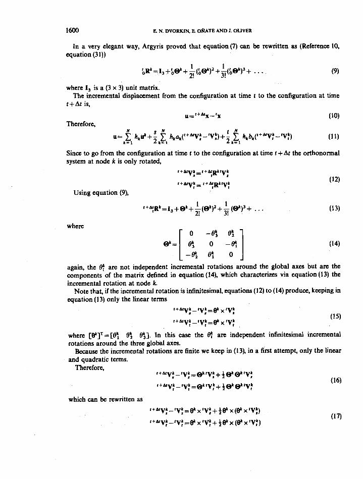
In a very elegant way, Argyris proved that equation (7) can be rewritten as (Reference 10, equation (3 1))

where I, is a (3 x 3) unit matrix. The incremental displacement from the configuration at time t to the configuration at time

t + At is,

,,='+&X-'X

Therefore,

Since to go from the configuration at time t to the configuration at time t + At the orthonormal system at node k is only rotated,

t +q: = t + & ~ k y k t I

Using equation (9),

where o -e: e:

ek=[_., ; -::I (14)

again, the 8: are not independent incremental rotations around the global axes but a n the components of the matrix detined in equation (l4), which characterizes via equation (13) the incremental rotation at node k.

Note that, if the incremental rotation is infinitesimal, equations (12) to (14) produce, keeping in equation (13) only the linear terms

where [8'lT=[8: 0: O i l . In this case the 8: are independent infinitesimal incremental rotations around the three global axes.

Because the incremental rotations are finite we keep in (1 3), in a first attempt, only the linear and quadratic terms.

Therefore, '+&Vf -'vf =)Ltv:+ +@k@"Vk

~ + ~ v : - t y : = @ k t y : + ~ @ k ) L t y : (16)

which can be rewritten as

LARGE DISPLACEMENT/ROTATION INCREMENTS

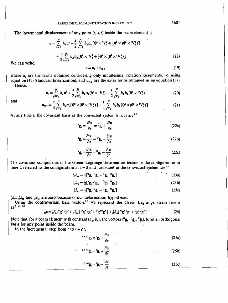
The incremental displacement of any point (r, s, t) inside the beam element is

We can write,

where us are the terms obtained considering only infinitesimal rotation increments, i.e. using equation (15) (standard linearization), and u,, are the extra terms obtained using equation (17).

Hence,

and

At any time t, the covariant basis of the convected system (r, s, t ) are1'

The covariant components of the Green-Lagrange deformation tensor in the configuration at time t, referred to the configuration at t = O and measured in the convected system are1'

&,; dc, and d$, are zero because of our deformation hypotheses. Using the contravariant base vectors1' we represent the Green-Lagrange strain tensor

BS2-4, 16

;E = ;grogr O g + ;&s[Og OgS + OgsOgl + cogr Og' + OgtOg] (24)

Note that, for a beam element with constant (a,, bk), the vectors (Og, Ogs, Og,), form an orthogonal basis for any point inside the beam.

In the incremental step from t to t +At,

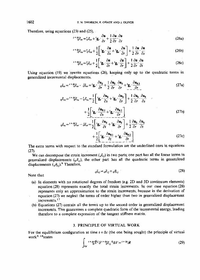
Therefore, using equations (23) and (25),

Using equation (19) we rewrite equations (26), keeping only up to the quadratic terms in generalized incremental displacements.

The extra terms with respect to the standard formulation are the underlined ones in equations (27).

We can decompose the strain increment in two parts; one part has all the linear terms in generalized displacements (oZij), the other part has all the quadratic terms in generalized displacements Therefore,

Note that

(a) In elements with no rotational degrees of freedom (e.g. 2D and 3D continuum elements) equation (28) represents exactly the total strain increments. In our case equation (28) represents only an approximation to the strain increments, because in the derivation of equation (27) we neglect the terms of order higher than two in generalized displacement increments."

(b) Equations (27) contain all the terms up to the second order in generalized displacement increments. This guarantees a complete quadratic form of the incremental energy, leading therefore to a complete expression of the tangent stiffness matrix.

3. PRINCIPLE O F VIRTUAL WORK

For the equilibrium configuration at time t + At (the one being sought) the principle of virtual workg. Isstates P

LARGE DISPLACEMENT/ROTATION INCREMENTS 1603

where O V is the volume in the initial configuration (t =O), '+%@ are the contravariant compo- nents measured in the convected system of the 2nd Piola-Kirchhoff stress tensor9* l 6 and '+A'W is the virtual work of the external loads acting on the configuration at time t +At.

When calculating '+A'&? it is important to notice that, although we are considering finite incremental rotations, the 6$ are infinitesimal, therefore the virtual work of the applied moments

NN is directly given by 1 M168: where NN is the total number of nodes in the model.

k = 1

Working out equation (29) the linearized equations of motion are obtained (Reference 9, Chapter 6).

4. INCREMENTAL FORMULATION FOR THE TIMOSHENKO BEAM ELEMENT

Using the kinematic equations presented in Section 2, we develop in this section the incremental Total Lagrangian Formulation9 for the Timoshenko beam element.

With the Newton-Raphson iteration scheme9 the equations for the ith iteration in a finite elements model are

For the displacements,

and for the rotations ( 1 +A:~k)(i) = (A t +A;~k)(i)(t +A;~k)(i- 1)

In the above '+aofK, is the linear part of the tangent stiffness matrix, '+%KNL the non-linear part of the tangent stiffness matrix, U the vector of generalized nodal incremental displacements,

the vector of generalized external nodal loads acting at t + At and

'+aofF the vector of generalized internal nodal loads acting at t + At, equivalent (in the virtual work sense) to the element stresses.

4.1. Tangent stzflness matrix

We define a vector

and the usual relation9

The matrix bBL is derived using equations (27) and (28). From the linearized equations of motion (Reference 9, Chapter 6) we obtain,

where ,C is a constitutive matrix formed with the contravariant components ,e'ik' of the

1604 E. N. DVORKIN. E. ORATE AND J. OLIVER

constitutive tensor that relates the increments of the contravariant components of the 2nd Piola-Kirchhoff stress tensor, measured in the convected system (,pi), with the increments of the covariant components of the Green-Lagrange strain tensor also measured in the convected system (,Eij). The incremental constitutive equation is, in matrix notation,

where

and

The curvilinear components ,Cijk' are calculated from the components in an orthonormal system (e*,, &j, kk):,

For elements of constant (a,, b,) we can define an orthonormal system Ci= Ogi/ 11 Ogi 11, and

where E is the Young's modulus, G is the shear modulus and K is the shear correction f a ~ t o r . ~ The linear part of the tangent stiffness matrix, as defined by equation (33), is the same for our

formulation and for the standard formulation. The difference will appear only in the non-linear part of the tangent stiffness matrix.

We derive the non-linear part of the tangent stiffness matrix from the equality (Reference 9, Chapter 6)

6UTbK,,U = b ~ i 6 0 i i j 'd V (39)

We define now the following matrices:

and also,

LARGE DISPLACEMENT/ROTATION INCREMENTS 1605

Matrices Br, 8,, 1, can be easily obtained using the kinematic relations presented in Section 2. Matrices $2, . . . , bni arise from the underlined terms in equations (27).

Being ki and k, the degrees of freedom corresponding to 8: and 8:; k- 1, . . . , N and i, 1= 1 , 2 , 3, the only non-zero terms in those matrices are

S f k t t k t b B : r ( k i , k0=8 hk, rakCtV:(l) fgr(i) + Vs(i) gr( l ) - ( Vs g r ) ( d i , + a,)]

t f k t +ih, rbkC vt(l) &a) + tv:(i)tgr(l) -Cv: ' g r ) ( d i ~ + d z i ) ] (42a)

S t k t t k t iP[:(kiy k l ) = 8 hk, rak[tv:( l) 'gs( i)+ vs(i) gs( l ) - ( V s ' g s ) ( d i l + d l i ) ]

t t k t + ghk. r b k C 'V:I )~~.~) + Vt(i) gs(l1 - ( ' V : . ' g s ) ( d i 1 + d l i ) ] . (424

S t k t t k t t k t 6 ' 3 4 9 k l ) = 8 hk, rak 1 Vs(,) + vs(i) gta -( V s g r ) ( d i 1 + d l i ) ]

where dij is the Kronecker delta. It is important to point out that the above defined matrices are symmetric. From equations ( 3 9 )

to ( 4 2 )

Note that

(a) The tangent stiffness matrix, dK = ;KL + ,'KNL is symmetric. (b) The second integral in equation ( 4 3 ) represents the difference with the tangent matrix as

obtained with the standard formulation.

1606 E. N. DVORKIN, E. ORATE AND J. OLIVER

4.2. Internal forces

The vector of generalized internal nodal forces equivalent in the virtual work sense to the element stresses is9

For calculating the stresses, the vectors 'V: and 'V: are updated using equation (7).

5. NUMERICAL EXPERIMENTATION

In this section we will compare for some simple examples the results obtained using the standard formulation and using the formulation presented in this paper. In order to avoid the locking problem,19 reduced numerical integration will be used along the r-direction.

It is important to point out that in beam elements reduced integration does not produce spurious zero energy modes,20 and therefore does not raise objections from the reliability view point.4

Full Newton-Raphson iterations are used in all the examples and the energy criteriong. 21 is used to test for convergence. Therefore, we stop the iterations when

where ETOL is an error tolerance defined for each case.

5.1. Cantilever beam under constant moment

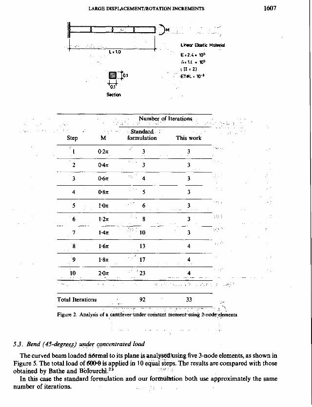
5.1.1. Analysis using 2-node elements. The cantilever is analysed using four 2-node elements, as shown in Figure 2. The total moment of 271, which for our case (EIIL = 2) corresponds to a total tip rotation of 71, is applied in 10 equal steps. Our formulation needs a total of 33 iterations to converge, against 92 iterations of the standard formulation. The coding differences for both formulations are very minor, therefore the number of iterations can be considered as an approximate indicator of the computational efficiency.

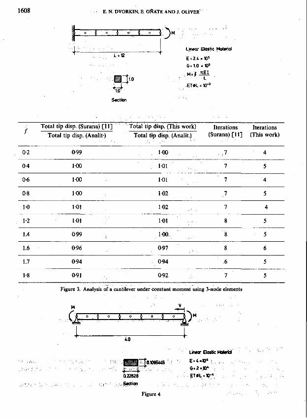
5.1.2. Analysis using 3-node elements. In the example shown in Figure 3 four 3-node elements are used. A total moment of 1.871 EIIL is applied in 10 steps, as indicated in the figure. Suranal also analysed this problem. In Figure 3 we display our results and the results reported in Reference 11; it is worth pointing out that, since different convergence criteria were used, the comparison of the number of iterations used by each formulation is not necessarily indicative of the effectiveness of each formulation.

5.2. Simply supported beam under constant moment

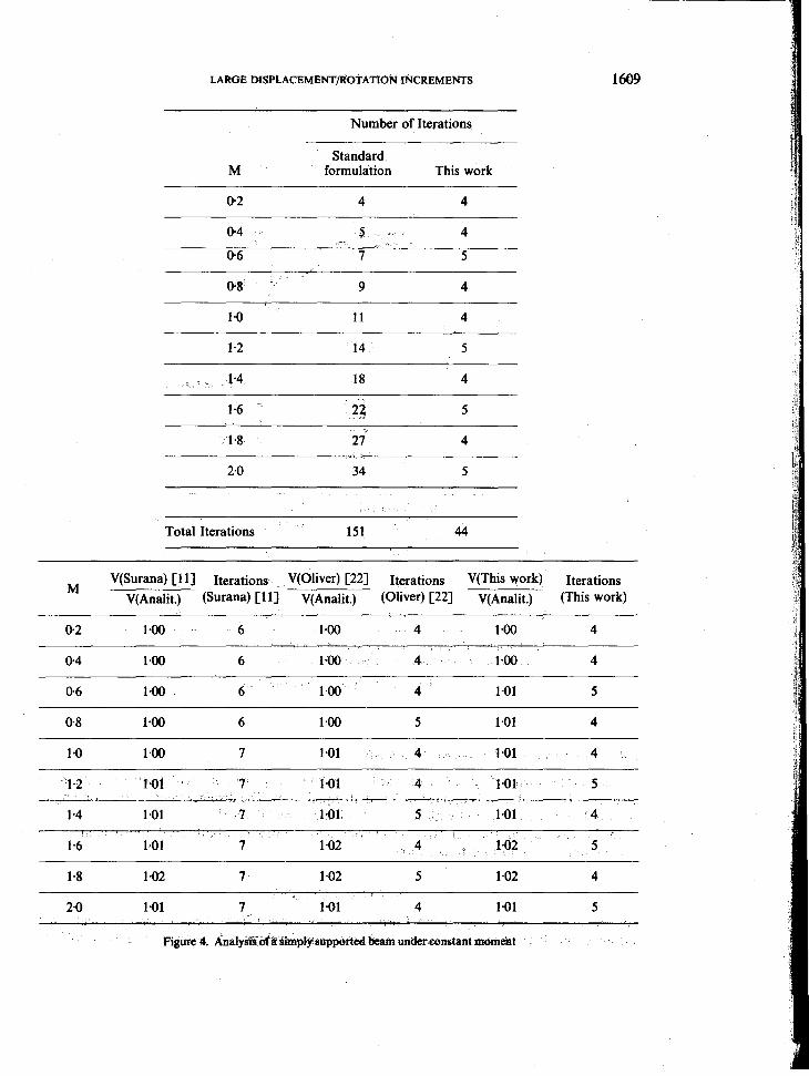
The beam is analysed using five 3-node elements, as shown in Figure 4. A total moment of 2.0 (which corresponds to a relative rotation of the beam ends of 2.5571) is applied in 10 equal steps. Our formulation needs a total of 44 iterations to converge against 151 iterations of the standard formulation.

Suranal and Oliver22 also analysed this problem. In Figure 4 we display their results and the present results. Again, different convergence criteria were used in the three cases and the comparison is not straightforward.

LARGE DISPLACEMENT/ROTATION INCREMENTS

Section

Number of Iterations

Standard Step M formulation This work

Total Iterations 92 33 . " P- - .. . " 1 d C I

Figure 2. Analysis of a cantilevcrbnrter constant m o m e n t - ~ - 2 . ~ elements

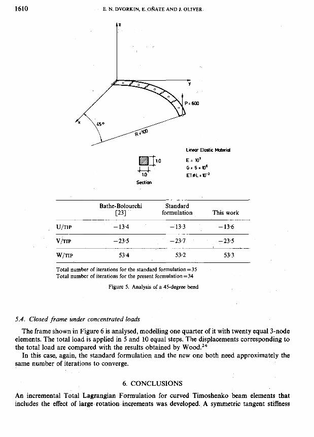
5.3. Bend (45-degrgq) under cpncentrated load

The curved beam loaded Mmal to its plane is a n a l y s ~ s i n g five 3-node elements, as shown in Figure 5. The total load of g00.Q id applied in 10 equal steps. The results are compared with those obtained by Bathe and Bol0urch3.~~

In this case the standard formulation and our formttktion both use approximately the same number of iterations.

E. N. DVORKIN, E. ORATE AND J. OLIVER'

Sect ion

Total tip disp. (Surana) [l'l] * Total tip disp. (This work) Iterations Iterations * Total tip disp. (Analit.) Total tip disp. (Analit.) (Surana) Clll (This work)

Figure 3. Analysis of a cantilever under constant moment using 3-node elements

3 *ion

Figure 4

LARGE MSPLACEMENTfltOTATION INCREMENTS

Number of Iterations

Standard M formulation This work

Total Iterations 151 44

M V(Surana) Clll Iterations V(Oliver) C221 Iterations V(This work) Iterations V(Ana1it.) (Surana) [ 1 11 V(Ana1it.) (Oliver) C221 V(Ana1it.) (This work)

2.0 1.01 7 1.01 4 1.01 5

Figure 4. AnafysEda $RnpEy$upported beam under constLnt m o m l t

E. N. DVORKIN, E. ORATE AND J. OLIVER

Linear Elastic Materid

section

Bathe-Bolourchi Standard C231 formulation This work

U/TIP - 13.4 - 13.3 - 13.6

V/TIP - 23.5 - 23-7 - 23-5

W/TIP 53.4 53.2 53.3

Total number of iterations for the standard formulation=35 Total number of iterations for the present formulation = 34

Figure 5. Analysis of a 45-degree bend

5.4. Closed frame under concentrated loads

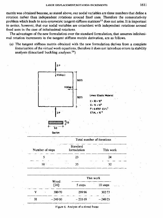
The frame shown in Figure 6 is analysed, modelling one quarter of it with twenty equal 3-node elements. The total load is applied in 5 and 10 equal steps. The displacements corresponding to the total load are compared with the results obtained by Wood.24

In this case, again, the standard formulation and the new one both need approximately the same number of iterations to converge.

6. CONCLUSIONS

An incremental Total Lagrangian Formulation for curved Timoshenko beam elements that includes the effect of large rotation increments was developed. A symmetric tangent stiffness

LARGE DISPLACEMENT~OTATION INCREMENTS 1611

matrix was obtained because, as stated above, our nodal variables are three numbers that define a rotation rather than independent rotations around fixed axes. Therefore the commutativity problem which leads to non-symmetric tangent stiffness matrices25 does not arise. It is important to notice, however, that our nodal variables are coincident with independent rotations around fixed axes in the case of infinitesimal rotations.

The advantages of the new formulation over the standard formulation, that assumes infinitesi- mal rotation increments in the tangent stiffness matrix derivation, are as follows.

(a) The tangent stiffness matrix obtained with the new formulation derives from a complete linearization of the virtual work equations, therefore it does not introduce errors in stability analyses (linearized buckling analyses.26)

Linear Elastic Material

Total number of iterations

Standard Number of steps formulation This work

5 23 24

This work Wood 1241 5 steps 10 steps

H -241.00 -235.19 - 24023

Figure 6. Analysis of a closed frame

1612 E. N. DVORKIN, E. ORATE AND J. OLIVER

(b) The complete tangent stiffness matrix assures quadratic convergence in the displacements norm when using full Newton-Raphson iteration^,^' therefore, in many cases when using the new formulation convergence is achieved with fewer iterations than when using the standard formulation. It is well known, however, that this should not always be the case, because in some problems iterating with a 'non-exact' tangent matrix may lead to a faster convergence. Also, some type of secant f~rmulation'~ could be developed to improve the efficiency of the analyses.

The same kind of formulation we presented for beam elements can be developed for C0 shell elements.

ACKNOWLEDGEMENT

E. N. Dvorkin acknowledges Prof. K. J. Bathe from M.I.T. for many important discussions on this topic.

REFERENCES

1. S. Ahmad, B. M. Irons and 0. C. Zienkiewicz, 'Analysis of thick and thin shell structures by curved finite elements', Int. j . numer. methods eng., 2, 419451 (1970).

2. E. N. Dvorkin and K. J. Bathe, 'A continuum mechanics based four-node shell element for general nonlinear analysis', Eng. Comp., 1, 77-88 (1984).

3. K. J. Bathe and E. N. Dvorkin, 'A four-node plate bending element based on Mindlin/Reissner plate theory and a mixed interpolation', Int. j. numer. methods eng., 21, 367-383 (1985).

4. K. J. Bathe and E. N. Dvorkin, 'A formulation of general shell elements-the use of mixed interpolation of tensorial components', Int. j. numer. methods eng., 22, 697-722 (1986).

5. J. Oliver and E. Oilate, 'A total Lagrangian formulation for the geometrically nonlinear analysis of structures using finite elements. Part I. Two-dimensional problems: shell and plate structures', Int. j. numer. methods eng., 20, 2253-2281 (1984).

6. J. Oliver and E. Ofiate, 'A total Lagrangian formulation for the geometrically nonlinear analysis of structures using finite elements. Part 11: arches, frames and axisymmetric shells', Int. j. nurner. methods eng., 23, 253-274 (1986).

7. K. C. Park and G. M. Stanley, 'A curved C0 shell element based on assumed natural-coordinate strains', J. Appl. Mech. ASME, 53, 278-290 (1986).

8. E. Hinton and H. C. Huang, 'A family of quadrilateral Mindlin plate elements with substitute shear strain fields', Comp. Struct., 23, 409-431 (1986).

9. K. J. Bathe, Finite Element Procedures in Engineering Analysis, Prentice-Hall, Englewood Cliffs, New Jersey, 1982. 10. J. Argyris, 'An excursion into large rotations', Comp. Methods Appl. Mech. Eng., 32, 85-155 (1982). 11. K. S. Surana, 'Geometrically nonlinear formulation for the curved shell elements', Int. j. numer. methods eng., 19,

581415 (1983). 12. J. C. Simo, 'A finite strain beam formulation. The three-dimensional dynamic problem. Part 1', Comp. Methods Appl.

Mech. Eng., 49, 55-70 (1985). 13. J. C. Simo and L. Vu Quoc, 'A three dimensional finite strain rod model. Part 11: computational aspects', Comp.

Methods Appl. Mech. Eng., 58, 79-1 16 (1986). 14. E. Oiiate, 'Una formulacion incremental para analisis de problemas de no linealidad geomktrica por el mktodo de 10s

elementos finitos' (in Spanish), Internal Report E.T.S. Ingenieros de Caminos, Universidad Politkcnica de Catalunya, Spain, 1986.

15. A. E. Green and W. Zerna, Theoretical Elasticity, 2nd edn, Oxford University Press, 1968. 16. L. E. Malvern, Introduction to the Mechanics of a Continuous Medium, Prentice-Hall, Englewood Cliffs, New Jersey,

1969. 17. K. J. Bathe, 'Finite element procedures for solids and structures-Nonlinear analysis', Video Course Study Guide,

M.I.T. Center for Advanced Engineering Study, 1986. 18. K. Washizu, Variational Methods in Elasticity and Plasticity, 3rd edn, Pergamon Press, London, 1982. 19. K. J. Bathe, E. N. Dvorkin and L. W. Ho, 'Our discrete-Kirchhoff and isoparametric shell elements for nonlinear

analysis-an assessment', Comp. Struct., 16, 89-98 (1983). 20. A. K. Noor and J. M. Peters, 'Mixed models and reduced/selective integration displacement models for nonlinear

analysis of curved beams', Int. j. numer. methods eng., 17, 615-631 (1981). 21. K. J. Bathe and A. P. Cimento, 'Some practical procedures for the solution of nonlinear finite element equations',

Comp. Methods Appl. Mech. Eng., 22, 59-85 (1980).

LARGE DISPLACEMENT/ROTATION INCREMENTS 1613

22. J. Oliver, 'Una formulaci6n cuasi-intrinseca para el estudio, por el mitodo de 10s elementos finitos, de vigas, arcos, placas y laminas sometidas a grandes corrimientos en rdgimen elastoplastico' (in Spanish), Doctoral Thesis, E.T.S. Ingenieros de Caminos, Universidad Politkcnica de Catalunya, Spain, 1982.

23. K. J. Bathe and S. Bolourchi, 'Large displacement analysis of three-dimensional beam structures', Int. j. numer. methods eng., 14, 961-986 (1979).

24. R. D. Wood, T h e application of finite element methods for geometrically nonlinear structural analysis', Ph.D. Thesis, University College of Swansea, Wales, U.K., 1973.

25. J. H. Argyris, H. Balmer, J. St. Doltsinis, P. C. Dunne, M. Haase, M. Kleiber, G. A. Malejannakis, H. P. Mlejnek, M. Miiller and D. W. Scharpf, 'Finite element method-the natural approach', Comp. Methods Appl. Mech. Eng., 17/18, 1-106 (1979)

26. K. J. Bathe and E. N. Dvorkin, 'On the automatic solution of nonlinear finite element equations', Comp. Struct., 17, 871-879 (1983).

27. E. Isaacson and H. B. Keller, Analysis of Numerical Methods, Wiley, New York, 1966.