Embed Size (px)
Citation preview
UNIVERSIT�E DE GEN�EVE
SCHOLA GENEVENSIS MDLIX
On a Model for Quantum Friction IIFermi’s Golden Rule and Dynamics at Positive Temperature
V. Jaksic 1 and C.-A. Pillet2
1Institute for Mathematics and its Applications, University of Minnesota, 514 Vincent Hall, 55455–0436 Minneapolis, Minnesota, U.S.A.2Departement de Physique Theorique, Universite de Geneve, CH–1211 Geneve 4, Switzerland
UGVA–DPT 1994/12–874
Abstract� We investigate the dynamics of an N -level system linearly coupled to a field of mass-less bosons at positive tempera-
ture. Using complex deformation techniques, we develop time-dependent perturbation theory and study spectral properties of the total
Hamiltonian. We also calculate the lifetime of resonances to second order in the coupling.
1. Introduction
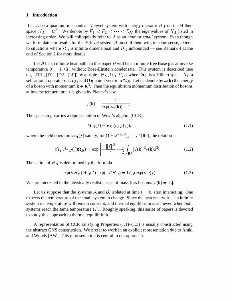
Let A be a quantum mechanical N -level system with energy operator HA on the Hilbertspace HA � CN . We denote by E1 � E2 � � � � � EM the eigenvalues of HA listed inincreasing order. We will colloquially refer to A as an atom or small system. Even thoughwe formulate our results for the N -level system A most of them will, in some sense, extendto situations where HA is infinite dimensional and HA unbounded — see Remark 4 at theend of Section 2 for more details.
Let B be an infinite heat bath. In this paper B will be an infinite free Bose gas at inversetemperature � � 1�kT , without Bose-Einstein condensate. This system is described (seee.g. [BR], [D1], [D2], [LP]) by a triple fHB ��B�HBg where HB is a Hilbert space, HB aself-adjoint operator on HB , and �B a unit vector in HB . Let us denote by �(k) the energyof a boson with momentum k � R3. Then the equilibrium momentum distribution of bosonsat inverse temperature � is given by Planck’s law
�(k) �1
exp(��(k))� 1�
The space HB carries a representation of Weyl’s algebra (CCR),
WB (f ) � exp(i�B(f ))� (1�1)
where the field operators �B (f ) satisfy, for (1 + ��1�2)f � L2(R3), the relation
(�B�WB (f )�B) � exp
��kfk
2
4� 1
2
ZR3jf (k)j2�(k)d3k
�� (1�2)
The action of HB is determined by the formula
exp(itHB)WB(f ) exp(�itHB) �WB (exp(it�)f )� (1�3)
We are interested in the physically realistic case of mass-less bosons: �(k) � jkj.Let us suppose that the systems A and B, isolated at time t � 0, start interacting. One
expects the temperature of the small system to change. Since the heat reservoir is an infinitesystem its temperature will remain constant, and thermal equilibrium is achieved when bothsystems reach the same temperature 1��. Roughly speaking, this series of papers is devotedto study this approach to thermal equilibrium.
A representation of CCR satisfying Properties (1.1)–(1.3) is usually constructed usingthe abstract GNS construction. We prefer to work in an explicit representation due to Arakiand Woods [AW]. This representation is central in our approach.
Fermi�s golden rule and dynamics at positive temperature 2
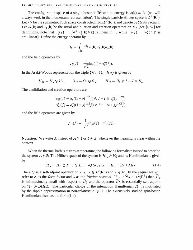
The configuration space of a single boson is R3 and its energy is �(k) � jkj (we willalways work in the momentum representation). The single particle Hilbert space is L2(R3).LetHb be the symmetric Fock space constructed fromL2(R3), and denote by�b its vacuum.Let ab(k) and a�b(k) be the usual annihilation and creation operators on Hb (see [RS2] fordefinitions, note that a�b(f ) �
Rd3k a�b (k)f (k) is linear in f , while ab(f ) � [a�b(f )]� is
anti-linear). Define the energy operator by
Hb �
ZR3d3k �(k) a�b(k)ab(k)�
and the field operators by
�b(f ) �1p2
(ab(f ) + a�b(f ))�
In the Araki-Woods representation the triple fHB��B �HBg is given by
HB � Hb �Hb� �B � �b � �b� HB � Hb � I � I �Hb�
The annihilation and creation operators are
aB(f ) � ab((1 + �)1�2f )� I + I � a�b(�1�2f )�
a�B(f ) � a�b((1 + �)1�2f )� I + I � ab(�1�2f )�
and the field operators are given by
�B (f ) �1p2
(aB(f ) + a�B(f ))�
Notation. We write A instead of A� I or I �A, whenever the meaning is clear within thecontext.
When the thermal bath is at zero-temperature, the following formalism is used to describethe system A + B: The Hilbert space of the system is HA �Hb and its Hamiltonian is givenby eH� � HA � I + I �Hb + Q� �b() � HA + Hb + eHI � (1�4)
There Q is a self-adjoint operator on HA, � L2(R3) and � R. In the sequel we willrefer to as the form factor and as the friction constant. If ��1�2 � L2(R3) then eHIis infinitesimally small with respect to eH0 and the operator eH� is essentially self-adjointon HA � D(Hb). The particular choice of the interaction Hamiltonian eHI is motivatedby the dipole approximation in non-relativistic QED. The extensively studied spin-bosonHamiltonian also has the form (1.4).
Fermi�s golden rule and dynamics at positive temperature 3
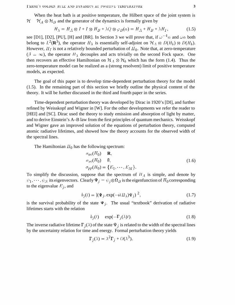
When the heat bath is at positive temperature, the Hilbert space of the joint system isH � HA �HB and the generator of the dynamics is formally given by
H� � HA � I + I �HB + Q� �B() � HA + HB + HI � (1�5)
see [D1], [D2], [PU], [H] and [BR]. In Section 3 we will prove that, if ��1 and � bothbelong to L2(R3), the operator H� is essentially self-adjoint on HA � D(Hb) � D(Hb).However, HI is not a relatively bounded perturbation of H0. Note that, at zero-temperature(� � �), the operator H� decouples and acts trivially on the second Fock space. Onethen recovers an effective Hamiltonian on HA � Hb which has the form (1.4). Thus thezero-temperature model can be realized as a (strong resolvent) limit of positive temperaturemodels, as expected.
The goal of this paper is to develop time-dependent perturbation theory for the model(1.5). In the remaining part of this section we briefly outline the physical content of thetheory. It will be further discussed in the third and fourth paper in the series.
Time-dependent perturbation theory was developed by Dirac in 1920’s [DI], and furtherrefined by Weisskopf and Wigner in [W]. For the other developments we refer the reader to[HEI] and [SC]. Dirac used the theory to study emission and absorption of light by matter,and to derive Einstein’s A–B law from the first principles of quantum mechanics. Weisskopfand Wigner gave an improved solution of the equations of perturbation theory, computedatomic radiative lifetimes, and showed how the theory accounts for the observed width ofthe spectral lines.
The Hamiltonian H0 has the following spectrum:
�ac(H0) � R�
�sc(H0) � ���pp(H0) � fE1� � � � � EMg�
(1�6)
To simplify the discussion, suppose that the spectrum of HA is simple, and denote by�1� � � � � �N its eigenvectors. Clearly�j � �j��B is the eigenfunction ofH0 correspondingto the eigenvalue Ej , and
bj(t) � j(�j� exp(�itH�)�j)j2� (1�7)
is the survival probability of the state �j . The usual “textbook” derivation of radiativelifetimes starts with the relation
bj(t) � exp(��j()t)� (1�8)
The inverse radiative lifetime �j() of the state�j is related to the width of the spectral linesby the uncertainty relation for time and energy. Formal perturbation theory yields
�j () � 2�j + O(3)� (1�9)
Fermi�s golden rule and dynamics at positive temperature 4
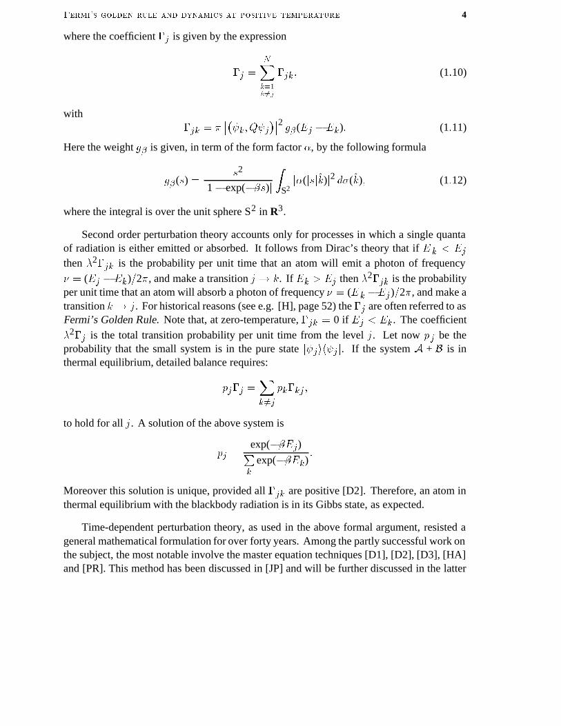
where the coefficient �j is given by the expression
�j �
NXk�1k ��j
�jk� (1�10)
with�jk �
����k� Q�j���2 g� (Ej � Ek)� (1�11)
Here the weight g� is given, in term of the form factor , by the following formula
g� (s) �s2
j1� exp(��s)jZ
S2j(jsj�k)j2 d�(�k)� (1�12)
where the integral is over the unit sphere S2 in R3.
Second order perturbation theory accounts only for processes in which a single quantaof radiation is either emitted or absorbed. It follows from Dirac’s theory that if E k � Ejthen 2
�jk is the probability per unit time that an atom will emit a photon of frequency
� � (Ej � Ek)�2 , and make a transition j � k. If Ek � Ej then 2�jk is the probability
per unit time that an atom will absorb a photon of frequency � � (Ek �Ej )�2 , and make atransition k � j. For historical reasons (see e.g. [H], page 52) the �j are often referred to asFermi’s Golden Rule. Note that, at zero-temperature, �jk � 0 if Ej � Ek. The coefficient
2�j is the total transition probability per unit time from the level j. Let now pj be the
probability that the small system is in the pure state j�jih�j j. If the system A + B is inthermal equilibrium, detailed balance requires:
pj�j �Xk ��j
pk�kj �
to hold for all j. A solution of the above system is
pj �exp(��Ej)Pk
exp(��Ek)�
Moreover this solution is unique, provided all �jk are positive [D2]. Therefore, an atom inthermal equilibrium with the blackbody radiation is in its Gibbs state, as expected.
Time-dependent perturbation theory, as used in the above formal argument, resisted ageneral mathematical formulation for over forty years. Among the partly successful work onthe subject, the most notable involve the master equation techniques [D1], [D2], [D3], [HA]and [PR]. This method has been discussed in [JP] and will be further discussed in the latter
Fermi�s golden rule and dynamics at positive temperature 5
papers in this series. Concerning the “usual” derivation of (1.8)–(1.12), note that Relation(1.8) cannot hold at zero-temperature for all times since the spectrum of eH� is bounded frombelow. Even at positive temperature it can hold only as an approximation and, to quote [SI],“it is often discussed fact in the physics literature that the usual “textbook derivation” of thetime-dependent series is internally inconsistent and there is not universal agreement amongphysicists concerning either the higher order terms in the series or the precise quantity whichis being approximated”.
The foundations of time-dependent perturbation theory for N -body, non-relativisticquantum systems, as well as the precise mathematical definition of resonance, were given in[SI]. We refer the reader to [SI] and [RS3] for a list of references concerning earlier work onthe subject. The notions introduced in [SI] have a natural extension to non-relativistic QED.The time-dependent perturbation series is supposed to describe the fate of the eigenvalues ofH0 (which are embedded in the continuous spectrum), after the perturbation HI is “turnedon”. It is expected that these eigenvalues will “dissolve”: There are � � 0 and � � 0 suchthat, for 0 � jj � �, the operator H� has no eigenvalues in ]Ej � ��Ej + �[. Let � be acontour enclosing the spectrum of H�. The formula
(�� exp(�itH�)�) �I�
exp(�itz)��� (z �H�)�1
�
� dz
2 i� (1�13)
relates the radiative lifetime of the state � to the poles of the function
R�(z) ���� (z �H�)�1
�
�� (1�14)
Following [SI], we now formulate the strategy for the analysis of the spectrum in the interval]Ej � ��Ej + �[, and the rigorous derivation of Relation (1.8): If the form factor issufficiently regular, there exists a dense subspace, E � H, on which the matrix elementsR�(z) have a meromorphic continuation from the upper half-plane onto the region O �
fz : jz � Ejj � �g. In O the functions R� are regular, except for a simple pole at a pointEj (), independent of the choice of � � E . If �j () � �2Im(Ej()) � 0, then H� haspurely absolutely continuous spectrum on ]Ej���Ej +�[. The resonance Ej() is expectedto be an analytic function of for jj � �. Finally, the first non-trivial coefficient in theTaylor expansion of Ej() should have an imaginary part given by Equations (1.9)–(1.12).One then can attempt to derive a formula for the decay of bj(t) using Relation (1.13). In firstapproximation one should get Equation (1.8).
For the zero-temperature model with massive bosons, this program was carried in part in[JP] and [OY]. However, the physically important case of mass-less bosons was beyond reach,except in some special cases [A1], [A2]. The difficulty, usually called infrared catastrophe,is related to the fact that there are vectors � in the domain of eH� which contain infinitely
Fermi�s golden rule and dynamics at positive temperature 6
many soft photons, i.e., (�� N�) � �. For many years no method could be designed toavoid this difficulty. Recently, V. Bach, J. Frohlich and I.M. Sigal [BFS] have developed asophisticated renormalization algorithm to address this problem. We refer reader to [HS] foran exposition of their results.
In this paper, the program presented above is carried out for the positive temperaturemodel defined by Equation (1.5).
Finally, we note that formal scattering theory relates (1.8)–(1.12) to experimental results[M]. It is therefore important to develop a scattering theory for the model (1.5). The methodexposed here yields some partial understanding of the scattering processes: We plan to do aperturbative analysis of the resonance scattering and to calculate the energy distribution ofphotons emitted and absorbed in transitions. This will be the subject of the fourth paper inthe series [JP2]. The investigation of the long time behavior of the interacting systemA+B,and in particular the study of the stability of the equilibrium states, is based on the fusion ofalgebraic and spectral methods. This will be the content of a third paper[JP1].
Acknowledgments. We are grateful to I. M. Sigal for suggesting the problem to us, and toV. Bach, R. Seiler, I. M. Sigal and H. Spohn for useful discussions. Part of this work hasbeen done while the first author was post-doctoral fellow at University of Toronto and visitorat University of Kentucky, Universite de Paris VII and Technische Universitat Berlin. Atvarious stages of this work, C.- A. P. was visiting the University of Toronto, and the Institutefor Mathematics and its Applications at the University of Minnesota. V. J. is grateful toV. Ivrii and J. Edward for much friendly support, and to P. Hislop, S. de Bievre, J. P. Gazeau,R. Seiler and V. Bach for their hospitality. The research of the first author was supported inpart by NSERC under grant OGP 0007901 and by Deutsche Forschungsgemeinschaft SFB288 Differentielgeometrie und Quantenphysik. The second author was supported by theFond National Suisse under grant 21–30607.
Fermi�s golden rule and dynamics at positive temperature 7
2. Statement of Results
We will need the following condition on the form factor .
(H1) (� + ��1) � L2(R3).
We begin with a self-adjointness statement for the generator of the dynamics (1.5).
Proposition 2.1. If Hypothesis (H1) is satisfied, then H� is essentially self-adjoint onHA �D(Hb)�D(Hb) for any � R.
To state our results, we need some additional notation. IfH is a Hilbert space, we denoteby H2(��H) the Hardy class of H-valued functions on the strip
S(�) fz : jIm(z)j � �g�The Hilbert space H2(��H) consists of all functions, f :S(�) � H, which are analytic inS(�) and satisfy
kfk2H2(��H) sup
jaj��
Z �
��kf (x + ia)k2
Hdx ��� (2�1)
Given a function f on R3, we define a new function ef on R S2 by the formula
ef (s� �k) ��jsj1�2 f (jsj�k) if s � 0,s1�2f (s�k) if s � 0.
(2�2)
With this notation, we can now formulate our central technical hypothesis:
(H2) There exists � � 0 such that e � H2(�� L2(S2))
The hypotheses (H1)–(H2) is satisfied, for example, by the function(k) �pjkj exp(�jkj2).
We may assume, without loss of generality, that � � 2 �� (see Section 3 for details).
Here is our main result.
Theorem 2.2. Suppose that (H1)–(H2) are satisfied. Then there exist a dense subspaceE � H and, for each � �]0� �[, a constant �(�) � 0 such that for �] � �(�)��(�)[ and��� � E , the functions
z ����� (H� � z)�1
�
�� (2�3)
have a meromorphic continuation from the upper half-plane onto the region
O fz : Im(z) � ��g�
Fermi�s golden rule and dynamics at positive temperature 8
The poles of the matrix elements (2.3) in O are independent of � and �. They are identicalto the eigenvalues of a quasi-energy operator �� on HA. This operator is analytic forjj � �(�), and has a power series representation of the form
�� � HA +�Xn�1
2n�
(2n)�
The first non-trivial coefficient in this expansion satisfies
Pj Im(�(2))Pj � PjQg� (HA � Ej )QPj� (2�4)
where Pj is the orthogonal projection on the eigenspace of HA corresponding to the eigen-value Ej , and g� is given in (1.12).
Remark 1. For any � � HA, one has � � �B � E .
Remark 2. Formula (2.4) is an obvious generalization of Equations (1.9)–(1.11) to de-generate eigenvalues. By first order perturbation theory, the eigenvalues of the operator�2Pj Im(�(2))Pj yield the coefficients of 2 in the expansion of the inverse eigenlifetimesof the eigenstates of energy Ej . In particular, if Ej non-degenerate, one easily gets thefollowing corollary.
Corollary 2.3. Suppose that (H1)–(H2) are satisfied, and let Ej be a simple eigenvalue ofHA. Then, for small , the quasi-energy operator �� has a unique simple eigenvalue Ej ()near Ej . This eigenvalue is analytic and satisfies
Ej () � Ej + 2a(2)j + O(4)�
Im(a(2)j ) � ��j�2�
where �j is given by Equations (1.9)–(1.12).
Theorem 2.2 and Proposition 4.1 in [CFKS] immediately yield the following
Corollary 2.4. Suppose that (H1)–(H2)are satisfied, and that the operatorsPj Im(�(2))Pj arenon-singular for 1 j M . Then there exists a constant � � 0 such that, for �]����[and �� 0, the operator H� has purely absolutely continuous spectrum filling the real axis.
We now turn to the dynamical aspects of the system.
Theorem 2.5. Suppose that (H1)–(H2) are satisfied. Then there exist a dense subspaceE � H and, for each � �]0� �[, a constant �(�) � 0 with the following property: For
Fermi�s golden rule and dynamics at positive temperature 9
jj � �(�) there are two maps W�� : E � HA such that, for any ��� � E , one has
(W�� ��W
+��) � (���) and��� exp(�itH�)�
���W�� �� exp(�i��t)W +
���
+ O(exp(��t))�
as t� +�.
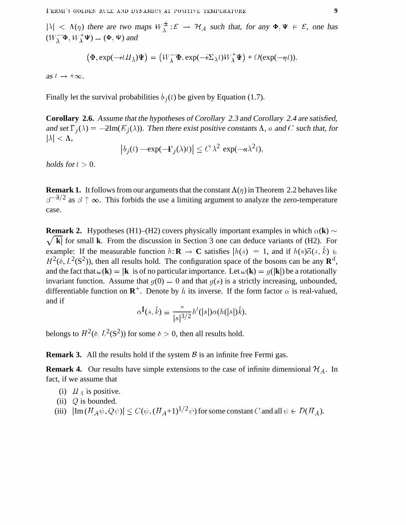
Finally let the survival probabilities bj(t) be given by Equation (1.7).
Corollary 2.6. Assume that the hypotheses of Corollary 2.3 and Corollary 2.4 are satisfied,and set �j () � �2Im(Ej()). Then there exist positive constants �, a and C such that, forjj � �, ��bj(t)� exp(��j()t)
�� C 2 exp(�a2t)�
holds for t � 0.
Remark 1. It follows from our arguments that the constant�(�) in Theorem 2.2 behaves like��3�2 as � � �. This forbids the use a limiting argument to analyze the zero-temperaturecase.
Remark 2. Hypotheses (H1)–(H2) covers physically important examples in which (k) �pjkj for small k. From the discussion in Section 3 one can deduce variants of (H2). For
example: If the measurable function h: R � C satisfies jh(s)j � 1, and if h(s)e(s� �k) �H2(�� L2(S2)), then all results hold. The configuration space of the bosons can be any Rd,and the fact that�(k) � jkj is of no particular importance. Let �(k) � g(jkj) be a rotationallyinvariant function. Assume that g(0) � 0 and that g(s) is a strictly increasing, unbounded,differentiable function on R+. Denote by h its inverse. If the form factor is real-valued,and if
�(s� �k) s
jsj3�2h�(jsj)(h(jsj)�k)�
belongs to H2(�� L2(S2)) for some � � 0, then all results hold.
Remark 3. All the results hold if the system B is an infinite free Fermi gas.
Remark 4. Our results have simple extensions to the case of infinite dimensional HA. Infact, if we assume that
(i) HA is positive.(ii) Q is bounded.
(iii) jIm (HA��Q�)j C(�� (HA+1)1�2�) for some constantC and all� � D(HA).
Fermi�s golden rule and dynamics at positive temperature 10
Then Proposition 2.1 holds with HA replaced by D(HA). Theorem 2.2 and Theorem 2.5also hold in this case, except that �� is now an analytic family of type A, and may havenon-discrete spectrum. This means that the matrix elements of the resolvent ofH� may haveessential singularities in O. However, for any bounded region R, there exists a constant�(��R) such that�� has purely discrete spectrum inR�O. In particular Corollary 2.3 holdstoo. Corollary 2.4 also holds locally, i.e., H� has purely absolutely continuous spectrum inR � R for jj � �(R). But we can assert that H� has no singular continuous spectrum forsmall . Finally if we make the following assumptions on the spectrum of HA,
(iv) The eigenvalues of HA have bounded multiplicity.(v) d0 lim inf
j��(Ej+1 � Ej) � 0.
Then one can choose the constant �(�) in Theorem 2.2 in such a way that �� has purelydiscrete spectrum. The reader will find a few remarks scattered in the remaining parts of thiswork to support these claims.
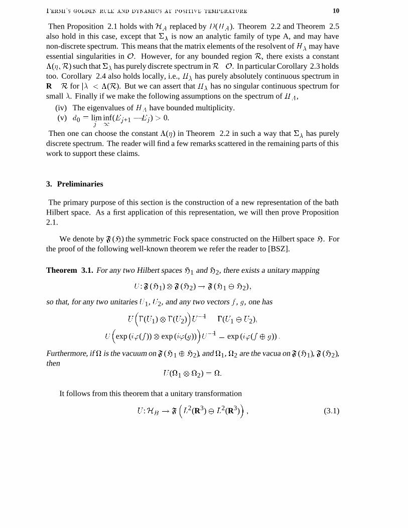
3. Preliminaries
The primary purpose of this section is the construction of a new representation of the bathHilbert space. As a first application of this representation, we will then prove Proposition2.1.
We denote by F (H) the symmetric Fock space constructed on the Hilbert space H. Forthe proof of the following well-known theorem we refer the reader to [BSZ].
Theorem 3.1. For any two Hilbert spaces H1 and H2, there exists a unitary mapping
U :F (H1)� F (H2)� F (H1 �H2)�
so that, for any two unitaries U1, U2, and any two vectors f , g, one has
U��(U1)� �(U2)
�U�1
� �(U1 � U2)�
U�
exp (i�(f ))� exp (i�(g))�U�1
� exp (i�(f � g)) �
Furthermore, if� is the vacuum on F (H1 �H2), and�1, �2 are the vacua on F (H1), F (H2),then
U (�1 � �2) � ��
It follows from this theorem that a unitary transformation
U :HB � F
�L2(R3)� L2(R3)
�� (3�1)
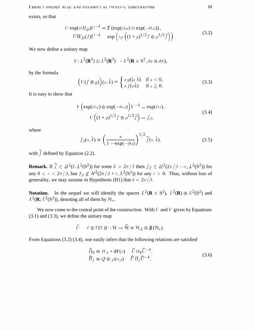
Fermi�s golden rule and dynamics at positive temperature 11
exists, so that
U exp(itHB)U�1� � (exp(it�)� exp(�it�)) �
UWB (f )U�1� exp
�i��
(1 + �)1�2f � �1�2f��
�(3�2)
We now define a unitary map
V :L2(R3)� L2(R3) � L2(R S2� ds� d�)�
by the formula �V (f � g)
�(s� �k)
�s g(jsj�k) if s � 0,s f (s�k) if s � 0.
(3�3)
It is easy to show that
V�
exp(it�)� exp(�it�)�V �1
� exp(its)�
V�
(1 + �)1�2f � �1�2f�� f� �
(3�4)
where
f� (s� �k)
s
1� exp(��s)1�2 ef (s� �k)� (3�5)
with ef defined by Equation (2.2).
Remark. If ef � H2(�� L2(S2)) for some � � 2 �� then f� � H2(2 �� � �� L2(S2)) for
any 0 � � � 2 ��, but f� �� H2(2 �� + �� L2(S2)) for any � � 0. Thus, without loss ofgenerality, we may assume in Hypothesis (H1) that � � 2 ��.
Notation. In the sequel we will identify the spaces L2(R S2), L2(R) � L2(S2) andL2(R;L2(S2)), denoting all of them by Hs.
We now come to the central point of the construction. WithU and V given by Equations(3.1) and (3.3), we define the unitary map
bU � I � �(V )U :H � bH HA � F (Hs) �
From Equations (3.2) (3.4), one easily infers that the following relations are satisfied
bH0 HA + d�(s) � bUH0bU�1�bHI Q� �(� ) � bUHIbU�1�
(3�6)
Fermi�s golden rule and dynamics at positive temperature 12
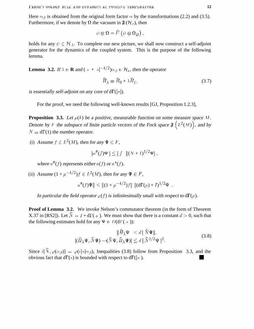
Here � is obtained from the original form factor by the transformations (2.2) and (3.5).Furthermore, if we denote by � the vacuum in F (Hs), then
� � � � bU �� ��B� �holds for any � � HA. To complete our new picture, we shall now construct a self-adjointgenerator for the dynamics of the coupled system. This is the purpose of the followinglemma.
Lemma 3.2. If � R and (jsj + jsj�1�2)� � Hs, then the operator
bH� bH0 + bHI � (3�7)
is essentially self-adjoint on any core of d�(jsj).
For the proof, we need the following well-known results [GJ, Proposition 1.2.3],
Proposition 3.3. Let �(k) be a positive, measurable function on some measure space M .
Denote by F the subspace of finite particle vectors of the Fock space F�L2(M )
�, and by
N d�(1) the number operator.
(i) Assume f � L2(M ), then for any � � F ,
ka#(f )�k kfk k(N + I)1�2�k�
where a#(f ) represents either a(f ) or a�(f ).
(ii) Assume (1 + ��1�2)f � L2(M ), then for any � � F ,
ka#(f )�k k(1 + ��1�2)fk k(d�(�) + I)1�2�k�
In particular the field operator �(f ) is infinitesimally small with respect to d�(�).
Proof of Lemma 3.2. We invoke Nelson’s commutator theorem (in the form of TheoremX.37 in [RS2]). Let bN � I + d�(jsj). We must show that there is a constant d � 0, such thatthe following estimates hold for any � � D(d�(jsj)):
kbH��k d kbN�k�j( bH��� bN�)� ( bN�� bH��)j d k bN1�2
�k2�(3�8)
Since i[ bN��(�)] � �(ijsj�), Inequalities (3.8) follow from Proposition 3.3, and theobvious fact that d�(s) is bounded with respect to d�(jsj).
Fermi�s golden rule and dynamics at positive temperature 13
Proof of Proposition 2.1. We start by observing that Hypothesis (H1) implies that(jsj + jsj�1�2)� � Hs. Therefore the conclusion of Lemma 3.2 holds. Let us define anauxiliary self-adjoint operator M on H by the formula
exp (iMt) � (exp(i�t))� � (exp(i�t)) �
Using the fundamental property of U (Theorem 3.1) and Definition (3.3) of V , one showsthat
M � bU�1d�(jsj)bU�It follows from Equation (3.6) and Lemma 3.2 thatH� �
bU�1 bH�bU is essentially self-adjoint
on any core of M . The fact that HA �D(Hb) � D(Hb) is such a core is well known (see[RS1], Theorem VIII.33).
Remark. Setting bN � I+HA+d�(jsj), the proofs of Lemma 3.2 and Proposition 2.1 extendto the situation where HA is unbounded, provided one makes the following assumptions:
(i) HA � 0.
(ii) Q is bounded with respect to H1�2A .
(iii) jIm (HA��Q�)j C(�� (HA+1)1�2�) for some constantC and all� � D(HA).
Of course one also has to replace HA with D(HA) in Proposition 2.1, and d�(jsj) withHA + d�(jsj) in Lemma 3.2.
Let us summarize the results of this section in
Theorem 3.4. There exists a unitary mapping bU :H � bH, such thatbUH�bU�1
� bH��
In the sequel we shall identify H with bH and H� with bH�, and always work in the newrepresentation. We would like to add a few comments concerning the above construction.
The simplest and most widely used complex-deformation technique is based on theAguilar-Combes theory and the group of dilation operators: [AC], [BC], [RS3] and [SI].The investigation of the zero-temperature model has been, so far, based on the second-quantization of the dilation group. This approach has been used in [OY], [JP], as well as ina recent work of Bach, Frohlich and Sigal [BFS]. In the mass-less case the infrared problemreflects itself in the fact that the eigenvalues fEjg are not uncovered by a dilation of the
Hamiltonian eH0: Regular perturbation theory does not apply directly. Since eHI is not arelatively compact perturbation of eH0, it is difficult to analyze the spectrum of eH� near Ej ,and to show that the matrix elements (1.14) have a meromorphic continuation across thecontinuous spectrum.
Fermi�s golden rule and dynamics at positive temperature 14
The resolution of the problem in the positive temperature case is based on the replacementof dilation analyticity with translation analyticity. The latter one originated in the study ofresonances of an atom in a homogeneous electric field (see [AH] and [HE] for an example).The formal connection between the two problems becomes transparent in Equation (3.6). Thecomplex deformation shifts the essential spectrum into the lower half-plane, and uncovers theeigenvalues fEjg. However, the domain of the Hamiltonian is modified by the deformation,and the bulk of the technical work below will center around the resolution of this difficulty.
4. Spectral Deformations and Fermi’s Golden Rule
Throughout this section we assume that Hypotheses (H1)–(H2) hold. For a � R, let u(a) bethe unitary translation group on Hs,�
u(a)f�
(s) � fa(s) f (s + a)� (4�1)
Denote by U (a) � �(u(a)) the second quantization of u(a). One easily shows that
U (a)�(f )U (�a) � �(f a)�
U (a)d�(s)U (�a) � d�(s) + aN�
where N d�(1) is the number operator on F (Hs). Thus, under a second quantizedtranslation, the operator H� transforms according to
H�(a) U (a)H�U (�a) � HA + d�(s) + Q� �(a�) + aN�
Remark that if f � H2(��H), Equation (4.1) defines a map from S(�) to L2(R) � H. Thefirst lemma in this section states some basic properties of such complex translations.
Lemma 4.1. Let 0 � �� � �, then the following holds:
(i) If f belongs to H2(��H) then its derivative f � belongs to H2(���H). Furthermore, onehas the bound
kf �kH2(���H) 1
� � �� kfkH2(��H)�
(ii) If f belongs to H 2(��H) then the map
S(�)� L2(R)�Ha �� fa
is analytic, and dfa
da � f �a.
Fermi�s golden rule and dynamics at positive temperature 15
(iii) If a� b � S(� �) then, for any f � H2(��H), one has the bound
kfa � fbkL2(R)�H ja� bj� � �� kfkH2(��H)�
Proof. Unless explicitly mentioned, all norms will refer to the space L2(R) � H. We firstprove (i). Since, by definition, f � H2(��H) implies that the function f :S(�) � H isanalytic, we only have to prove the bound on the derivative f �. Denote by �f � L2(R� dr)�Hthe Fourier transform of f � L2(R� ds)�H, then the norm (2.1) can be expressed as
kfkH2(��H) � supjaj��
���exp(ar)�f��� �
Therefore we have
kf �kH2(���H) � supjaj���
���r exp(ar)�f���
suprR
��r exp��(�� ��)jrj��� sup
jaj���
���exp�ar + (� � ��)jrj� �f��� �
and an explicit calculation leads to the desired inequality:
kf �kH2(���H) 1
e(� � ��) supjaj��
���exp(jarj)�f��� p
2e
1� � �� kfkH2(��H)�
Using the same notation, we now prove (ii). Assume that jIm(a)j � � � � �. Then, for smallh � C, ���fa+h � fa � hf �a
��� � ���exp(iar) (exp(ihr)� 1� ihr) �f���
suprR
��exp��Im(a)r� � �jrj� (exp(ihr)� 1� ihr)
�� ���exp(��jrj)�f��� �
and another simple calculation gives���fa+h � fa � hf �a��� o(h) kfkH2(��H)� (4�2)
as h� 0, which is the desired estimate. To prove (iii) remark that, as a consequence of (ii),we have
fa � fb � (b� a)Z 1
0f �a+t(b�a)
dt�
Therefore (i) gives���fa � fb��� jb� aj sup
0t1
���f �a+t(b�a)��� jb� aj kf �kH2(���H)
jb� aj� � �� kfkH2(��H)�
Fermi�s golden rule and dynamics at positive temperature 16
as required.
Let now a � S(�) be complex, and define
HI (a) Q� 1p2
�a(a�) + a�(a� )
��
H�(a) HA + d�(s) + HI (a) + aN�(4�3)
These operators are well defined on the dense subspace
D � D(N ) �D(d�(s))�
One easily checks that, as an operator on D, H�(a) satisfies the relation
H�(a)� � H��(a)� (4�4)
Therefore, H�(a) is closable for each (� a) � CS(�). We use the same symbol to denoteits closure. The following proposition summarizes some simple facts about the family ofclosed operators fH0(a) : a � Cg.
Proposition 4.2. Assume that a � C, then the following holds:
(i) For any � � D one has
kH0(a)�k2� kH0(Re(a))�k2 + jIm(a)j2kN�k2�
(ii) If Ima �� 0, then H0(a) is a normal operator satisfying
D(H0(a)) � D�H0(a)� � H0(a)�
(iii) The spectrum of H0(a) is given by
�(H0(a)) � fna + t :n � 1� 2� � � � ; t � Rg � �(HA)�
Proof. Remark that, on the sector N � n, the operator H0(a) reduces to the normal operator
H(n)0 (a) HA + s1 + � � � + sn + na�
A simple calculation immediately yields Identity (i). From this identity one easily showsthat, if Im(a) �� 0,
D �
n� � f�(n)g :�(n) � D(H (n)
0 (a));P
nkH(n)0 (a)�(n)k2 ��
o�
Fermi�s golden rule and dynamics at positive temperature 17
and it follows that H0(a) is a closed normal operator on D. The last assertion in (ii) , and(iii) both follow from corresponding statements about H (n)
0 (a).
The next result provides us with the necessary control of the interaction HI (a).
Lemma 4.3. Let a � S(�), and Im(a) �� 0. Then the interaction HI (a) is infinitesimallysmall with respect to H0(a).
Proof. By Cauchy-Schwarz inequality,
kQ� a#(f )�k2 kQ2�k ka#(f )�a#(f )�k�
Applying a well-known trick we obtain, for any � � 0,
kQ� a#(f )�k 12�kQ2
�k +�
2ka#(f )�a#(f )�k�
By Proposition 3.3, we further get
kQ� a#(f )�k 12�kQ2
�k +�
2kfk2k(N + 2)�k�
Finally, since Im(a) �� 0, the first statement of Proposition 4.2 and Equation (4.3) lead to
kHI (a)�k �kH0(a)�k + Ck�k�for appropriate C � 0.
Let us introduce the strips
S�(�) � fz : 0 � �Im(z) � �g�We are now ready to prove some basic properties of the deformed operator H�(a).
Proposition 4.4. Assume that (� a) � CS�(�), then:
(i) The following identities hold,
D(H�(a)) � D�H�(a)� � H�(a)�
(ii) The spectrum of H�(a) satisfies
�(H�(a)) � fz : Im(z) D(� a)g�
Fermi�s golden rule and dynamics at positive temperature 18
where D(� a) is given by
D(� a) 12
jRe()j� � jIm(a)j jIm(a)j1�2 + jIm()j jIm(a)j�1�2
2kQk2 k�k2
H2(�)�
Furthermore, if Im(z) � D(� a), one has the bound����H�(a)� z��1
��� 1Im(z)�D(� a)
�
(iii) The map(� a) �� H�(a)
from C S�(�) to the closed operators on H, is an analytic family of type A in eachvariable separately.
Remark. A similar statement holds for (� a) � CS+(�).
To prove Proposition 4.4, we need the following simple facts (see e.g., [K] Chapter V,Section 3.2): If T is a closed operator on a Hilbert space H, the convex set
(T ) � f(�� T�) : � � D(T )� k�k � 1g�
is called numerical range of T . Let us denote byN(T ) the closure of this set.
Lemma 4.5. Let T be a closed operator on a Hilbert space H, such that D(T ) � D(T �).Then
�(T ) � N(T )�
and, for z � C nN(T ), one has the bound���(T � z)�1��� 1
dist (z�N(T ))� (4�5)
Proof. Let � � D(T ) be a unit vector, then Cauchy-Schwarz inequality implies
k(T � z)�k � jz � (�� T�)j � (4�6)
It follows that T � z is one-to-one if z �� N(T ). Arguing similarly we see that (T � z)� isone-to-one if z �� N(T �). Since N(T �) � N(T ), we conclude that T � z has a bounded,everywhere defined inverse for z �� N(T ). Estimate (4.5) follows from Inequality (4.6).
Fermi�s golden rule and dynamics at positive temperature 19
Proof of Proposition 4.4. The first assertion is a simple consequence of Lemma 4.3. Toestablish the second assertion, we set
bD(� a) sup Im�N(H�(a))
�� (4�7)
The assertion will follow from Lemma 4.5, provided we can show that bD(� a) D(� a).To this end we first observe that, since real translations are unitary, we can choose a � �i�with 0 � � � �. Then a simple calculation shows that
Im�H�(a)
�� ��N + �Q� �(g)� (4�8)
where
�g 12i
�a� � �a�
�� kgk � 1�
Denote by P the orthogonal projection on g, and set P� � 1�P . By construction, we haveN � d�(P )� d�(P�) � a�(g)a(g)�N�, and (4.8) splits into a direct sum
Im�H�(a)
�� ��
�a�(g)a(g)� �
�Q� �(g)
� N�
��
In the above formula, we recognize the sum of a (shifted) harmonic oscillator and a numberoperator. Completing the square in the first term, and performing a unitary transformation,we can rewrite
Im�H�(a)
�� �� I �
�N0 �N�� +
�2
2�Q2 � I�
where N0 is a simple harmonic oscillator. Therefore we have
��Im�H�(a)
���
��n +
�2
2�q2 :n � 0� 1� � � � ; q � �(Q)
��
which, by Definition (4.7), means
bD(� a) �2
2�kQk2�
We conclude by estimating � with the help of Lemma 4.1. To prove the last assertion, wefirst claim that, for fixed � C and � � D, the vector valued function a �� H�(a)� isanalytic. In fact, with
�H�(a)�a
N + Q� 1p2
�a���
�a�
+ a����
a��
�
Fermi�s golden rule and dynamics at positive temperature 20
Proposition 3.3 (i) implies����H�(a + h)��H�(a)�� h�H�(a)�a
�
���� � O�ka+h
� � a� � h�a�k��
By Lemma 4.1 (ii), the right hand side of the last inequality is o(h), proving the claim. SinceStrong analyticity in for fixed a is obvious, type A analyticity now follows from the firsttwo assertions of the proposition.
Remark. If we replace D by D(N ) � D(HA + d�(s)), the proof of Proposition 4.2 extendsto unbounded HA. The same remark holds for the proof of Lemma 4.3 and Proposition 4.4provided Q is bounded.
We now further investigate the spectrum of H�(a). We will denote by P(�) the openhalf-plane fz : Im(z) � �g.
Theorem 4.6. There exists a constant� � 0 such that, for (� a) � CS�(�), the followingstatements hold:
(i) Ifjj � � jIm(a)j� (4�9)
then the spectrum of the operatorH�(a) in the half-plane P(Im(a)+ j�j�
) is purely discreteand independent of a.
(ii) If
jj � 14� jIm(a)j�
then the spectral projection P�(a) associated to the spectrum of H�(a) in P(Im(a) + j�j�
)is analytic in and satisfies the bound
kP�(a)� P0(a)k � 3�jIm(a)j �
Proof. Remark that, by Proposition 4.2 and Lemma 4.3, the resolvent formula
�H�(a)� z
��1��H0(a)� z
��1�
1 + HI (a)�H0(a)� z
��1��1
� (4�10)
holds for small , as long as z belongs to a cone of the form fz : 0 � c1 � jzj � c2 Im(z)g.We organize the proof of Theorem 4.6 in two steps: First we will extend the domain of
Fermi�s golden rule and dynamics at positive temperature 21
validity of Formula (4.10) by refining our estimate on the productH I (a)(H0(a)�z)�1. Thenwe will invoke analytic perturbation theory to control the spectrum.
Applying Proposition 3.3 (i), we get���HI (a)�H0(a)� z
��1��� p
2 kQk k�kH2(�)
���(N + 1)1�2 �H0(a)� z��1
��� �Since N and H0(a) are commuting normal operators, it is rather easy to compute the normof T � (N + 1)1�2(H0(a)� z)�1. On the sector N � 0, the operator T reduces to
T (0)��HA � z
��1�
and therefore,
kT (0)k � 1dist(z� �(HA))
� (4�11)
On the other hand if z � E + i� and a � � � i�, the sector N � n � 0 reduces T to
T (n)�
pn + 1
(HA + s1 + � � � + sn + n� �E)� i (�n + �)�
It follows that
kT (n)k �pn + 1
j�n + �j � (4�12)
Since kTk � supn�0 kT (n)k, Equations (4.11) and (4.12) lead, after an elementary analysis,to the bound
kTk ���
p2
dist(z�(H0(a))) if�� � � � 3�;1
2p�(���)
if � � 3�.(4�13)
If we set
� 12 kQk k�kH2(�)
�
G(a� �) �z : Im(z) � Im(a); dist
�z� �(H0(a))
�� �
��
one easily verifies that, for � � jIm(a)j, the bound (4.13) implies
supzG(a�)
���HI (a)�H0(a)� z
��1��� jj
� �� (4�14)
Consequently, if jj � � �, the identity (4.10) holds on G(a� �). Moreover the followingestimate holds for N � 0
supzG(a�)
�������z �H�(a)��1�
N�1Xj�0
�z �H0(a)
��1�HI (a)
�z �H0(a)
��1�j������ 1
�
���
�N1�
���
��
Fermi�s golden rule and dynamics at positive temperature 22
It follows that any z in the set
P(Im(a)) n �(HA) �� 0
G(a� �)�
is in the resolvent set of H�(a) for small . Therefore, the discrete spectrum of H0(a) isstable, and analytic perturbation theory applies. The first statement of Theorem 4.6 follows,except for the independence of the eigenvalues on the parameter a. Fix (0� a0) satisfying(4.9). Since H�0
(a) is an analytic family in a, its discrete eigenvalues are (branches of)analytic functions with at most algebraic singularities in a neighborhood of a0. On theother hand, H�0
(a0) and H�0(a) are unitarily equivalent if a� a0 is real. Thus the discrete
eigenvalues are independent of a.
To prove the second statement, assume that 2� � jIm(a)j and jj � ��. Let �� be thecontours defined by fz : Im(z) � �Im(a)�2g, and set � �+ � ��. We formally define
P�(a) �I�
dz
2 i
�z �H�(a)
��1� (4�15)
We shall prove below that, as a weak integral, and after extraction of explicit zeroth and firstorder terms, the above integral becomes absolutely convergent. Therefore, P�(a) is analyticand, by a standard argument, is the spectral projection of H�(a) corresponding to the part ofits spectrum contained in the strip bounded by �+ and ��. Iterating the resolvent identity weget
P�(a) � P0 + �(1)(a) + 2�
(2)� (a)� (4�16)
where
P0 P0(a) � I � � (�� � )��
(1)(a) I�
dz
2 i
�H0(a)� z
��1HI (a)
�H0(a)� z
��1�
�(2)� (a) �
I�
dz
2 i
�H0(a)� z
��1HI (a)
�H�(a)� z
��1HI (a)
�H0(a)� z
��1�
An explicit calculation shows that �(1)(a) can be written as
�(1)(a) �
1i
Z �
��exp(��jtj)�t dt� (4�17)
where
�t �P0 exp(iH0t)HI (a) exp(�iH0t) for t � 0,exp(iH0t)HI (a) exp(�iH0t)P0 for t � 0.
Fermi�s golden rule and dynamics at positive temperature 23
Another simple calculation yields
k�tk � 2�3�2��1�
Thus we conclude from Equation (4.17) that����(1)(a)��� jj
��� (4�18)
To estimate �(2)� (a), we proceed as follows: By Cauchy-Schwarz inequality we have, for
any ��� � H,�������(2)� (a)�
���� supz�
���HI (a)�H�(a)� z
��1HI (a)
��� �(�) �(�)� (4�19)
where
�(�)2 Z�
djzj2
����H0(a)� z��1
�
���2�
By the spectral theorem (recall that H0(a) is normal), this quantity is easily seen to bebounded by
�(�) s
2�k�k� (4�20)
We now deal with the supremum in Expression (4.19). We start by the simpler case � 0.There we can apply the method which leads to Inequality (4.14). Leaving the details to thereader, we quote the resulting bound
supz�
���HI (a)�H0(a)� z
��1HI (a)
��� 2
�2 �� (4�21)
Using the resolvent formula (4.10), a simple calculation shows that
HI (a)�H�(a)� z
��1HI (a) ��
1� HI (a)�H0(a)� z
��1��1
HI (a)�H0(a)� z
��1HI (a)�
Therefore, Inequalities (4.14) and (4.21) yield
supz�
���HI (a)�H�(a)� z
��1HI (a)
��� 2
�2 �
1�
jj��
�1�
Optimizing the last expression over �, and combining it with the estimate (4.20) gives thedesired bound ���2
�(2)� (a)
��� 2jj��
2 1�
2jj��
�1� (4�22)
Fermi�s golden rule and dynamics at positive temperature 24
Putting together (4.18) and (4.22), we finally get
kP�(a)� P0(a)k x
1 + 2x1� 2x
�
with x jj��� � 1�2, from which the required inequality follows easily.
Remark. In the case of unbounded HA and bounded Q, the above argument shows that thespectrum of H�(a) decomposes into a first part �0 � fz : jIm(z)j jj��g, and a secondpart in fz : Im(z) Im(a) + jj��g. Statement (ii) of Theorem 4.6 still holds in this case.However �0 need not be purely discrete. In general we can only assert that, given anybounded region R, there exists a �(a�R) such that the spectrum in �0 � R is discrete forjj � �(a�R). On the other hand, if we assume that the spectrum of HA is well separated
d0 lim infj��
(Ej+1 �Ej ) � 0�
and has bounded multiplicity, then one easily shows that �0 is discrete provided jj �� min(jIm(a)j� d0).
The previous result allows us to apply reduction theory to the discrete spectrum ofresonances, and to construct the quasi-energy operator by transforming Ran(P�(a)) back toHA with a linear isomorphism S�(a). We follow here the developments of [HP]. If
jj � � jIm(a)j�4� (4�23)
Theorem 4.6 implies thatkP�(a)� P0k � 1�
It immediately follows that the maps
P0 : Ran(P�(a)) � HA�
P�(a) :HA � Ran(P�(a))�
are isomorphisms. Consequently, setting
T� P0P�(a)P0� (4�24)
one easily checks that the operator
S�(a) T�1�2� P0P�(a)�
from Ran(P�(a)) to HA has inverse
S�(a)�1 P�(a)P0T�1�2� �
Fermi�s golden rule and dynamics at positive temperature 25
We use the isomorphism S�(a) to transport the reduced operator P�(a)H�(a)P�(a) back inthe space HA. A simple calculation yields
�� S�(a)P�(a)H�(a)P�(a)S�(a)�1� T
�1�2� M�T
�1�2� � (4�25)
withM� P0P�(a)H�(a)P�(a)P0� (4�26)
Finally we remark that since U (a)P0 � P0U (a) � P0 for any a � C, the operators T� andM� are independent of a as long as Condition (4.23) holds.
The following lemma explores some properties of the quasi-energy (4.25).
Proposition 4.7. The quasi-energy operator depends analytically on for jj � � jIm(a)j�4.It has a Taylor series of the form
�� � HA +�Xn�1
�(2n)2n�
The first non-trivial coefficient in this expansion is
�(2) �1
2
Xj
�Qh�(Ej �HA)QPj + PjQh� (Ej �HA)Q
��
where the function h� (z), analytic in P(��), is given for Im(z) � 0 by the formula
h� (z) Z
R S2
j� (s� �k)j2s� z
ds d�(�k)�
Proof. The analyticity of T� follows from its definition (4.24) and Theorem 4.6 (ii). By the
same result, kT� � Ik � 1 holds for jj � � jIm(a)j�4. Therefore T�1�2� is also analytic.
The Taylor series of T� is obtained by inserting the Neumann series for the resolvent ofH�(a) in Equation (4.15). In this way we obtain
T� � I +�Xn�1
T (n)n�
with coefficients given by
T (n) I�
dz
2 i
�z �HA
��1P0HI (a)
��z �H0(a)
��1HI (a)
�n�1P0�z �HA
��1�
Fermi�s golden rule and dynamics at positive temperature 26
In a completely similar way we can write
M� � HA +�Xn�1
M (n)n�
with the following coefficients
M (n) I�
dz
2 iz�z �HA
��1P0HI (a)
��z �H0(a)
��1HI (a)
�n�1P0�z �HA
��1�
The fact that odd powers of drop out of this expansions is an easy consequence of photonnumber conservation (recall that P0 projects on the zero photon subspace). By Definition(4.25), the first non-trivial coefficient in the Taylor series of �� is
�(2)�M (2) � 1
2
�T (2)HA + HAT
(2)��
An explicit calculation gives
�(2)�
12
I�
dz
2 i
�K(z)
�z �HA
��1 +�z �HA
��1K(z)
�� (4�27)
whereK(z) P0HI (a)
�z �H0(a)
��1HI (A)P0�
Remark that the resolvent in K(z) is restricted to the one-photon sector, therefore K(z) isanalytic in P(Im(a)). Another explicit calculation shows that, for Im(z) � 0,
K(z) � �12Qh� (z �HA)Q�
Therefore, applying the Cauchy integral formula to Equation (4.27) gives
�(2)� �1
2
Xj
Qh� (Ej �HA)QPj + PjQh� (Ej �HA)Q�
as required.
Remark 1. In the case of unbounded HA and bounded Q, the quasi-energy is an analyticfamily of type A with domain D(HA). In fact one can show that the commutator [HA� T�]is bounded. It follows easily that �� �HA is bounded and analytic.
Remark 2. The above argument also yields an expression for the Lamb shifts of the energylevel Ej .
Fermi�s golden rule and dynamics at positive temperature 27
Now that we have got some understanding of the family fH�(a) j a � S�(�)g, we shallrelate it to the physical operator H�. This is the content of the next result.
Lemma 4.8. For � R and Im(z) sufficiently large, we have
s� limIm(a)�0
�H�(a)� z
��1��H�(Rea)� z
��1�
Proof. Clearly we may assume Re(a) � 0. Note that, by Proposition 4.4 (ii), the resolventof H�(a) is uniformly bounded as Im(a) � 0 when � R. Therefore, it suffices to showstrong convergence on a dense subspace. We will prove that
limIm(a)�0
�����H�(a)� z��1 � �H� � z
��1�
(N + 1)�1��� � 0�
As usual, we denote by F � F (Hs) the subspace of finite particle vectors. We define
D0 ��H�(a)� z
�� :� � HA � (F �D(d�(jsj)))� �
which is a dense subspace by Proposition 4.4 and the remark which follows it. SinceHA� (F �D(d�(jsj))) is a core of d�(jsj), it is also a core of H� by Lemma 3.2. It followsthat, for � � D0,
L(a)� �H�(a)� z
��1�� �H� � z
��1�
��H� � z
��1 �H� �H�(a)
� �H�(a)� z
��1�
��H� � z
��1Q� 1p
2
�a(� � �a� ) + a�(� � a�)
�� aN
�H�(a)� z
��1��
Since D0 is dense, the above formula extends by continuity to arbitrary �. By Proposition3.3 (i) and Lemma 4.1 (iii), we further have
kL(a)(N + 1)�1k jajIm(z)
�1 +
p2jj kQk k�kH2(�)
� � jIm(a)j
����(N + 1)�H�(a)� z
��1(N + 1)�1��� �
We end the proof by showing that (N + 1)�H�(a)� z
��1 (N + 1)�1 is uniformly boundedas Im(a) � 0. Indeed, a simple calculation shows that
(N + 1)H�(a) (N + 1)�1� H�(a) + Q� 1p
2
�a�(a� )� a(�a�)
�(N + 1)�1�
which, by Proposition 3.3, is a uniformly bounded perturbation of H�(a).
Fermi�s golden rule and dynamics at positive temperature 28
Remark. If HA is unbounded and Q bounded, we only need to replaceHA by D(HA) in thedefinition of D0, and the above proof still holds.
Let E � F (Hs) be the set of entire vectors for the group U (a). We recall that Econsists of all � � F (Hs) such that the vector-valued function U (a)� has an entire analyticextension. Define E � HA�E. It follows from the Paley-Wiener theorem that E is a denseset of vectors in H.
Proof of Theorem 2.2. For ��� � E , � R and Im(z) sufficiently large, the function
a �� f (a) �U (a)��
�H�(a)� z
��1U (a)�
��
is analytic in S�(�). Since it is obviously independent of Re(a), f is actually constant onS�(�). Let us show that f is continuous onS�(�) � R. Indeed,
f (a)� f (0) ������H�(a)� z
��1 � �H� � z��1
��
�+�U (a)��
�H�(a)� z
��1 (U (a)� I)��
+�
(U (a)� I)���H�(a)� z
��1�
��
The first term vanishes as Im(a) � 0 by Lemma 4.8. The two other terms also tend to zero inthis limit since � and � are entire vectors for translations, and (H�(a)� z)�1 is uniformlybounded. Therefore, f (a) � f (0) holds onS�(�) � R. Since by Theorem 4.6 the function
z ���U (a)��
�H�(a)� z
��1U (a)�
��
is meromorphic on P(Im(a) + jj��), it does provide the required extension. The propertiesof this extension follow from Theorem 4.6 and Proposition 4.7. In particular the expressionfor Im(�(2)) is obtained using the well known formula
Im
1
x� io
� i �(x)�
in the definition of h� (z).
Remark. Here again we did not use the fact that HA is bounded. Of course the constructedextension will only be meromorphic if the spectrum of �� is discrete.
Proof of Theorem 2.5. Let ��� � E , and define
f (t) ��� exp(�iH�t)�
��
Fermi�s golden rule and dynamics at positive temperature 29
Then for Im(z) � 0, the Fourier-Laplace transform
bf (z) Z �
0f (t) exp(izt)dt �
1i
����H� � z
��1�
��
is well defined. For any � � 0, the inverse relation
f (t) �Z �
��bf (E + i�) exp(�i(E + i�)t)
dE
2 � (4�28)
holds for t � 0. Now let us set a � �i� with 0 � � � �, and assume that 4� � jIm(a)j,and jj � ��. As in the proof of Theorem 2.2, bf (z) has an extension to the lower half-planegiven by bf (z) �
1i
�U (a)��
�H�(a)� z
��1U (a)�
��
By the resolvent identity and estimates (4.20) (4.14), bf belongs to the Hardy class of the stripfz :�� + � � Im(z) � ��g. It follows that we can rewrite the inversion formula (4.28) as
f (t) �I�
bf (z) exp(�izt) dz2
+Z �
��bf (E � i(�� ��)) exp(�i(E � i(�� ��))t)dE
2 �
where the contour � is as in the proof of Theorem 4.6, and �� � �. The first term in theabove expression is easily identified as
fd(t) ��U (a)�� S�(a)�1 exp(�i��t)S�(a)U (a)�
��
whereas the second term is of the order exp(�(�� ���)t) for ��� � ��. The proof is complete.To prove Corollary 2.6 we only need the additional observation that, if �j (� a) denote theeigenvector of H�(a) associated to the eigenvalue Ej (), then�
�i(� a)��j(0� a)�� �i�j + O(2)�
Remark. The above proof does not use the fact that HA is bounded.
References
[A1] Arai, A.: On a model of harmonic oscillator coupled to a quantized, mass-less, scalar field, I. J. Math. Phys. ��, 2539(1981).
Fermi�s golden rule and dynamics at positive temperature 30
[A2] Arai, A.: On a model of harmonic oscillator coupled to a quantized, mass-less, scalar field, II. J. Math. Phys. ��, 2549(1981).
[AC] Aguilar, J. and J.M. Combes: A class of analytic perturbations for one-body Schrodinger Hamiltonians. Commun. Math.Phys. ��, 269 (1971).
[AH] Avron, J.E. and I. Herbst: Spectral and scattering theory of Schrodinger operators related to the Stark effect. Commun.Math. Phys. ��, 239 (1977).
[AW] Araki, H. and E.J. Woods: Representation of the canonical commutation relations describing a nonrelativistic infinite freeBose gas. J. Math. Phys. �, 637 (1963).
[BC] Balslev, E. and J.M. Combes: Spectral properties of many-body Schrodinger operators with dilation analytic interactions.Commun. Math. Phys. ��, 280 (1971).
[BE] Bethe, H.A.: The electromagnetic shift of energy levels. Phys. Rev. ��, 339 (1947).
[BR] Bratteli, O. and D. Robinson: Operator Algebras and Quantum Statistical Mechanics II, New York, Springer (1981).
[BFS] Bach, V., J. Frohlich and I.M. Sigal: (In preparation).
[BSZ] Baez, J.C., I.E. Segal and Z. Zhou: Introduction to Algebraic and Constructive Quantum Field Theory, Princeton, Prince-ton University Press (1991).
[C] Cannon, J.T.: Infinite volume limits of the canonical free Bose gas states on the Weyl algebra. Commun. Math. Phys. ��,89 (1973).
[CFKS] Cycon, H., R. Froese, W. Kirsch and B. Simon: Schrodinger Operators, Berlin, Springer Verlag (1987).
[D1] Davies, E.B: Quantum Theory of Open Systems, London, Academic Press (1976).
[D2] Davies, E.B.: Markovian master equations. Commun. Math. Phys. ��, 91 (1974).
[D3] Davies, E.B.: Markovian master equations, II. Math. Ann. ���, 147 (1976).
[DI] Dirac, P.A.M.: The quantum theory of the emission and absorption of radiation. Proc. Royal Soc. London, Series A ���,243 (1927).
[GJ] Glimm, J. and A. Jaffe: Quantum field theory models. In Statistical Mechanics and Quantum Field Theory, (C. DeWittand R. Stora). New York–London–Paris, Gordon and Breach (1970).
[H] Haag, R.: Local Quantum Physics, Berlin, Springer Verlag (1993).
[HA] Haake, F.: Statistical Treatment of Open Systems by Generalized Master Equations, (Springer Tracts in Modern Physics66). Berlin–Heidelberg–New York, Springer Verlag (1973).
[HE] Herbst, I.: Exponential decay in Stark effect. Commun. Math. Phys. ��, 197 (1980).
[HEI] Heitler, W.: The Quantum Theory of Radiation, London, Oxford University Press (1954).
[HP] Hunziker, W. and C.-A. Pillet: Degenerate asymptotic perturbation theory. Commun. Math. Phys. �, 219 (1983).
[HS] Hubner, M. and H. Spohn: Radiative decay: Non perturbative approaches. Preprint.
[JP] Jaksic, V. and C.-A. Pillet: On a model for quantum friction I. Resonances and dynamics at zero-temperature. (To appear).Anal. Inst. H. Poincare
[JP1] Jaksic, V. and C.-A. Pillet: On a model for quantum friction III. Return to equilibrium. (In preparation).
[JP2] Jaksic, V. and C.-A. Pillet: On a model for quantum friction IV. Scattering theory. (In preparation).
Fermi�s golden rule and dynamics at positive temperature 31
[JS] Jaksic, V. and J. Segert: Exponential approach to the adiabatic limit and Landau-Zener formula. Rev. Math. Phys. �, 529(1992).
[K] Kato, T.: Perturbation Theory for Linear Operators, New York, Springer Verlag (1966).
[LP] Lewis, J.T. and J.V. Pule: The equilibrium state of the free boson gas. Commun. Math. Phys. �, 1 (1974).
[M] Messiah, A.: Quantum Mechanics, Vol I and II, Amsterdam, North Holland (1961).
[OY] Okamoto, T. and K. Yajima: Complex scaling technique in non-relativistic massive QED. Ann. Inst. H. Poincare ��, 31(1985).
[PR] Prigogine, I.: The statistical interpretation of non-equilibrium entropy. In The Boltzmann Equation, Theory, and Applica-tions, (E.G.D. Cohen and W. Thirring). Berlin–Heidelberg–New York, Springer Verlag (1973).
[PU] Pule, J.V.: The Bloch equations. Commun. Math. Phys. ��, 241 (1974).
[RS1] Reed, M. and B. Simon: Methods of Modern Mathematical Physics, I. Functional Analysis, London, Academic Press (1980).
[RS2] Reed, M. and B. Simon: Methods of Modern Mathematical Physics, II. Fourier Analysis, Self-Adjointness, London, Aca-demic Press (1975).
[RS3] Reed, M. and B. Simon: Methods of Modern Mathematical Physics, IV. Analysis of Operators, London, Academic Press(1978).
[SI] Simon, B.: Resonances in N-body quantum systems with dilation analytic potentials and the foundations of time-dependentperturbation theory. Ann. Math. ��, 247 (1973).
[SC] Schwinger, J.: Selected Papers on Quantum Electrodynamics, New York, Dover (1958).
[W] Weisskopf, V. and E.P. Wigner: Berechnung der naturlichen Linienbreite auf Grund der Diracschen Lichtheorie. Z. Phys.�, 54 (1930).