On a Linear Programming Approach to the Discrete …math.univ-lyon1.fr/~masnou/fichiers/publications/avignon.pdfnonlinear boundary value problem into an integer linear ... integer

On a Linear Programming Approach to theDiscrete Willmore Boundary Value Problem

and Generalizations

Thomas Schoenemann1, Simon Masnou2, and Daniel Cremers3

1 Center for Mathematical Sciences, Lund University, Sweden, [email protected] Universite de Lyon, Universite Lyon 1, CNRS UMR 5208, Institut Camille Jordan,

Villeurbanne, France, [email protected] Department of Computer Science, Technical University of Munich, Garching,

Germany, [email protected]

Abstract. We consider the problem of finding (possibly non connected)discrete surfaces spanning a finite set of discrete boundary curves in thethree-dimensional space and minimizing (globally) a discrete energy in-volving mean curvature. Although we consider a fairly general class ofenergies, our main focus is on the Willmore energy, i.e. the total squaredmean curvature. Most works in the literature have been devoted to theapproximation of a surface evolving by the Willmore flow and, in par-ticular, to the approximation of the so-called Willmore surfaces, i.e., thecritical points of the Willmore energy. Our purpose is to address the deli-cate task of approximating global minimizers of the energy under bound-ary constraints. The main contribution of this work is to translate thenonlinear boundary value problem into an integer linear program, usinga natural formulation involving pairs of elementary triangles chosen ina pre-specified dictionary and allowing self-intersection. The reason forsuch strategy is the well-known existence of algorithms that can computeglobal minimizers of a large class of linear optimization problems, how-ever at a significant computational and memory cost. The case of integerlinear programming is particularly delicate and usual strategies consistin relaxing the integral constraint x ∈ {0, 1} into x ∈ [0, 1] which is easierto handle. Our work focuses essentially on the connection between theinteger linear program and its relaxation. We prove that:– One cannot guarantee the total unimodularity of the constraint ma-

trix, which is a sufficient condition for the global solution of therelaxed linear program to be always integral, and therefore to be asolution of the integer program as well;

– Furthermore, there are actually experimental evidences that, in somecases, solving the relaxed problem yields a fractional solution.

These facts indicate that the problem cannot be tackled with classicallinear programming solvers, but only with pure integer linear solvers.Nevertheless, due to the very specific structure of the constraint matrixhere, we strongly believe that it should be possible in the future to de-sign ad-hoc integer solvers that yield high-definition approximations tosolutions of several boundary value problems involving mean curvature,in particular the Willmore boundary value problem.

2 T. Schoenemann, S. Masnou, and D. Cremers

Keywords: mean curvature, Willmore functional, integer linear programming,relaxation, total unimodularity

1 Introduction

The Willmore energy of an immersed compact oriented surface f : Σ → RNwith boundary ∂Σ is defined as

W(f) =

∫Σ

|H|2dA+

∫∂Σ

κ ds

where H is the mean curvature vector on Σ, κ the geodesic curvature on ∂Σ,and dA, ds the induced area and length metrics on Σ, ∂Σ. The Willmore en-ergy of surfaces with or without boundary plays an important role in geom-etry, elastic membranes theory, strings theory, and image processing. Amongthe many concrete optimization problems where the Willmore functional ap-pears, let us mention for instance the modeling of biological membranes, thedesign of glasses, and the smoothing of meshed surfaces in computer graphics.The Willmore energy is the subject of a long-standing research not only due toits relevance to some physical situations but also due to its fundamental prop-erty of being conformal invariant, which makes it an interesting substitute tothe area functional in conformal geometry. Critical points of W with respect tointerior variations are called Willmore surfaces. They are solutions of the Euler-Lagrange equation δW = 0 whose expression is particularly simple when N = 3:∆H+2H(H2−K) = 0, being K the Gauss curvature. It is known since Blaschkeand Thomsen [23] that stereographic projections of compact minimal surfaces inS3 ⊂ R4 are always Willmore surfaces in R3. However, Pinkall exhibited in [22]an infinite series of compact embedded Willmore surfaces that are not stereo-graphic projections of compact embedded minimal surfaces in S3. Yet Kusnerconjectured [17] that stereographic projections of Lawson’s g-holed tori in S3should be global minimizers of W among all genus g surfaces. This conjecture isstill open, except of course for the case g = 0 where the round sphere is knownto be the unique global minimizer.

The existence of smooth surfaces that minimize the Willmore energy span-ning a given boundary and a conormal field has been proved by Schatzle in [27].Following the notations in [27], we consider a smooth embedded closed orientedcurve Γ ⊂ RN together with a smooth unit normal field nΓ ∈ NΓ and wedenote as ±Γ and ±nΓ their possible orientations. We assume that there ex-ist oriented extensions of ±Γ , ±nΓ , that is, there are compact oriented sur-faces Σ−, Σ+ ⊂ RN with boundary ∂Σ± = ±Γ and conormal vector fieldcoΣ± = ±nΓ on ∂Σ±. We also assume that there exists a bounded open setB ⊃ Γ such that the set

{Σ± oriented extensions of (Γ, nΓ ), Σ+ connected ,

Σ+ ∪Σ− ⊂ B, W(Σ+ ∪Σ−) < 8π}

The Discrete Willmore Boundary Problem 3

is not empty. The condition on energy ensures that Σ+ ∪Σ− is an embedding.

It follows from [27], Corollary 1.2, that the Willmore boundary problem as-sociated with (Γ, nΓ ) in B has a solution, i.e., there exists a compact, oriented,connected, smooth surface Σ ⊂ B with ∂Σ = Γ , coΣ = nΓ on ∂Σ, and

W (Σ) = min{W (Σ), Σ smooth, Σ ⊂ B, ∂Σ = Γ, coΣ = nΓ on ∂Σ}

There have been many contributions to the numerical simulation of Willmoresurfaces in space dimension N = 3. Among them, Hsu, Kusner and Sullivanhave tested experimentally in [16] the validity of Kusner’s conjecture: startingfrom a triangulated polyhedron in R3 that is close to a Lawson’s surface ofgenus g, they let it evolve by a discrete Willmore flow using Brakke’s SurfaceEvolver [6] and check that the solution obtained after convergence is W-stable.Recent updates that Brakke brought to its program give now the possibility totest the flow with various discrete definitions of the mean curvature. Mayer andSimonett [19] introduce a finite difference scheme to approximate axisymmet-ric solutions of the Willmore flow. Rusu [26] and Clarenz et al. [8] use a finiteelements approximation of the flow to compute the evolution of surfaces withor without boundary. In both works, position and mean curvature vector aretaken as independent variables, which is also the case of the contribution byVerdera et al. [33], where a triangulated surface with a hole in it is restoredusing the following approach: by the coarea formula, the Willmore energy (actu-ally a generalization to other curvature exponents) is replaced with the energyof an implicit and smooth representation of the surface, and the mean curvatureterm is replaced by the divergence of an unknown field that aims to representthe normal field. Droske and Rumpf [9] propose a finite element approach tothe Willmore flow but replace the standard flow equation by its level set for-mulation. The contribution of Dziuk [10] is twofold: it provides a finite elementapproximation to the Willmore flow with or without boundary conditions thatcan handle as well embedded or immersed surfaces (turning the surface probleminto a quasi-planar problem), and a consistency result showing the convergenceof both the discrete surface and the discrete Willmore energy to the continuoussurface and its energy when the approximated surface has enough regularity.Bobenko and Schroder [4] use a difference strategy: they introduce a discretenotion of mean curvature for triangulated surfaces computed from the circlescircumscribed to each triangle that shares with the continuous definition a fewproperties, in particular the invariance with respect to the full Mobius group inR3. This discrete definition is vertex-based and a discrete flow can be derived.Based also on several axiomatic constraints but using a finite elements frame-work, Wardetzky et al. [34] introduce an edge-based discrete Willmore energyfor triangulated surfaces. Olischlager and Rumpf [21] introduce a two step timediscretization of the Willmore flow that extends to the Willmore case, at leastformally, the discrete time approximation of the mean curvature motion dueto Almgren, Taylor, and Wang [2], and Luckhaus and Sturzenhecker [18]. Thestrategy consists in using the mean curvature flow to compute an approxima-tion of the mean curvature and plugging it in a time discrete approximation of


the Willmore flow. Grzibovskis and Heintz [14], and Esedoglu et al. [11] discusshow 4th order flows can be approximated by iterative convolution with suitablekernels and thresholding.

While all the previous approaches yield approximations of critical pointsof the Willmore energy, our motivation in this paper is to approximate globalminimizers. This is an obviously nontrivial task due to the high nonlinearity andnonconvexity of the energy. Yet, for the simpler area functional, Sullivan [31]has shown with a calibration argument that the task of finding minimal surfacescan be turned into a linear problem. Even more, when a discrete solution isseeked among surfaces that are union of faces in a cubic grid partition of R3,he proved that the minimization of the linear program is equivalent to solving aminimum-cost circulation network flow problem, for which efficient codes havebeen developed by Boykov and Kolmogorov [5] after Ford and Fulkerson [12].Sullivan [31] did not provide experiments in his paper but this was done recentlyby Grady [13], with applications to the segmentation of medical images.

The linear formulation that we propose here is based on two key ideas: theconcept of surface continuation constraints that has been pioneered by Sulli-van [31] and Grady [13], and the representation of a triangular surface usingpairs of triangles. With this representation and a suitable definition of discretemean curvature, we are able to turn into a linear formulation the task of mini-mizing discrete representations of any functional of the form

Wϕ(Σ) =

∫Σ

ϕ(x, n,H)dA

among discrete immersed surfaces with boundary constraints:

∂Σ = Γ, coΣ = nΓ on ∂Σ.

In the expression of Wϕ(Σ), x denotes the space variable, n the normal vectorfield on Σ and H the mean curvature vector. The linear problem we obtaininvolves integer-valued unknowns and does not seem to admit any simple graph-based equivalent. We will therefore discuss whether classical strategies for linearoptimization can be used.

The paper is organized as follows: in Section 2 we discuss both the cho-sen representation of surfaces and the definition of discrete mean curvature. InSection 3 we present a first possible approach yielding a quadratic energy. Wepresent in Section 4 our linear formulation and discuss whether it can be tackledby classical linear optimization techniques.

2 Discrete Framework

2.1 Triangular Meshes from a Set of Pre-defined Triangles

The equivalence shown by Sullivan between finding minimal surfaces and solvinga flow problem holds true for discrete surfaces defined as a connected set of cellfaces in a cellular complex discrete representation of the space. We will consider


here polyhedral surfaces defined as union of triangles with vertices in (a finitesubset of) the cubic lattice εZ3 where ε = 1

n is the resolution scale. Not allpossible triangles are allowed but only those respecting a specified limit on themaximal edge length. We assume that each triangle, as well as each triangle edge,is represented twice, once for each orientation. We let I denote the collection oforiented triangles, N = |I| its cardinality, and M the number of oriented triangleedges. The constrained boundary is given as a contiguous oriented set of triangleedges. The orientation of the boundary constrains the spanning surfaces sincewe will allow only spanning triangles whose orientation is compatible.

In this framework, one can represent a triangular mesh as a binary indicatorvector x = {0, 1}N where 1 means that the respective triangle is present inthe mesh, 0 that it is not. Obviously, not all binary indicator vectors can beassociated with a triangular surface since the corresponding triangles may notbe contiguous. However, as discussed by Grady [13] and, in a slightly differentsetting, by Sullivan [30, 31], it is possible to write in a linear form the constraintthat only binary vectors that correspond to surfaces spanning the given boundaryare considered. We will see that using the same approach here turns the initialboundary value problem into a quadratic program. Another formulation will benecessary to get a linear problem.

2.2 Admissible Indicator Vectors: A First Attempt

To define the set of admissible indicator vectors, we first consider a relationshipbetween oriented triangles and oriented edges which is called incidence: a triangleis positive incident to an edge if the edge is one of its borders and the two agreein orientation. It is negative incident if the edge is one of its borders, but in theopposite orientation. Otherwise it is not incident to the edge. For example, thetriangle in Figure 1 is positive incident to the edge e1, negative incident to e2and e3 and not incident to e4.

e4e3

e2

e1 Fig. 1. Incidence of oriented trianglesand edges. e1 is positively incident tothe oriented triangle, e2 and e3 are neg-atively incident, and e4 is not incidentto the triangle.

Being defined as above the set of N oriented triangles and their M orientededges, we introduce the matrix B = (bij)i∈{1,··· ,N}

j∈{1,··· ,M}whose element bij gives

account of the incidence between triangle i and edge j. More precisely


bij =

1 if edge i is an edge of triangle j with same orientation

−1 if edge i is an edge of triangle j with opposite orientation

0 otherwise.

The knowledge of which edges are present in the set of prescribed boundarysegments is expressed as a vector r ∈ {−1, 0, 1}M with

rj =

1 if the oriented boundary contains the edge j

with agreeing orientation

−1 if the oriented boundary contains the edge −jwith opposing orientation

0 otherwise.

With these notations, we can now describe the equation system defining thata vector x ∈ {0, 1}N encodes an oriented triangular mesh with the pre-specifiedoriented boundary. This system has one equation for each edge. If the edgeis not contained in the given boundary, this equation expresses that, amongall triangles indicated by x that contain the edge, there are as many triangleswith same orientation as the edge as triangles with opposite orientation. If theedge is contained in the boundary with coherent orientation, there must beone more positive incident triangle than negative incident. If it is contained withopposite orientation, there is one less positive than negative incident. Altogetherthe constraint for edge j can be expressed as the linear equation∑

i

bij xi = rj

and the entire system asB x = r. (1)

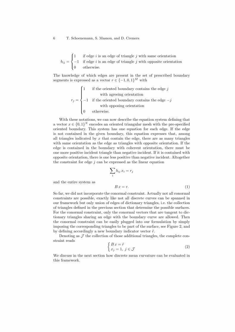
So far, we did not incorporate the conormal constraint. Actually not all conormalconstraints are possible, exactly like not all discrete curves can be spanned inour framework but only union of edges of dictionary triangles, i.e. the collectionof triangles defined in the previous section that determine the possible surfaces.For the conormal constraint, only the conormal vectors that are tangent to dic-tionary triangles sharing an edge with the boundary curve are allowed. Thenthe conormal constraint can be easily plugged into our formulation by simplyimposing the corresponding triangles to be part of the surface, see Figure 2, andby defining accordingly a new boundary indicator vector r.

Denoting as J the collection of those additional triangles, the complete con-straint reads {

B x = rxj = 1, j ∈ J (2)

We discuss in the next section how discrete mean curvature can be evaluated inthis framework.


Fig. 2. The boundary and conormal constraints can be imposed by pre-specifying suit-able triangles to be part of the surface.

2.3 Discrete Mean Curvature on Triangular Meshes

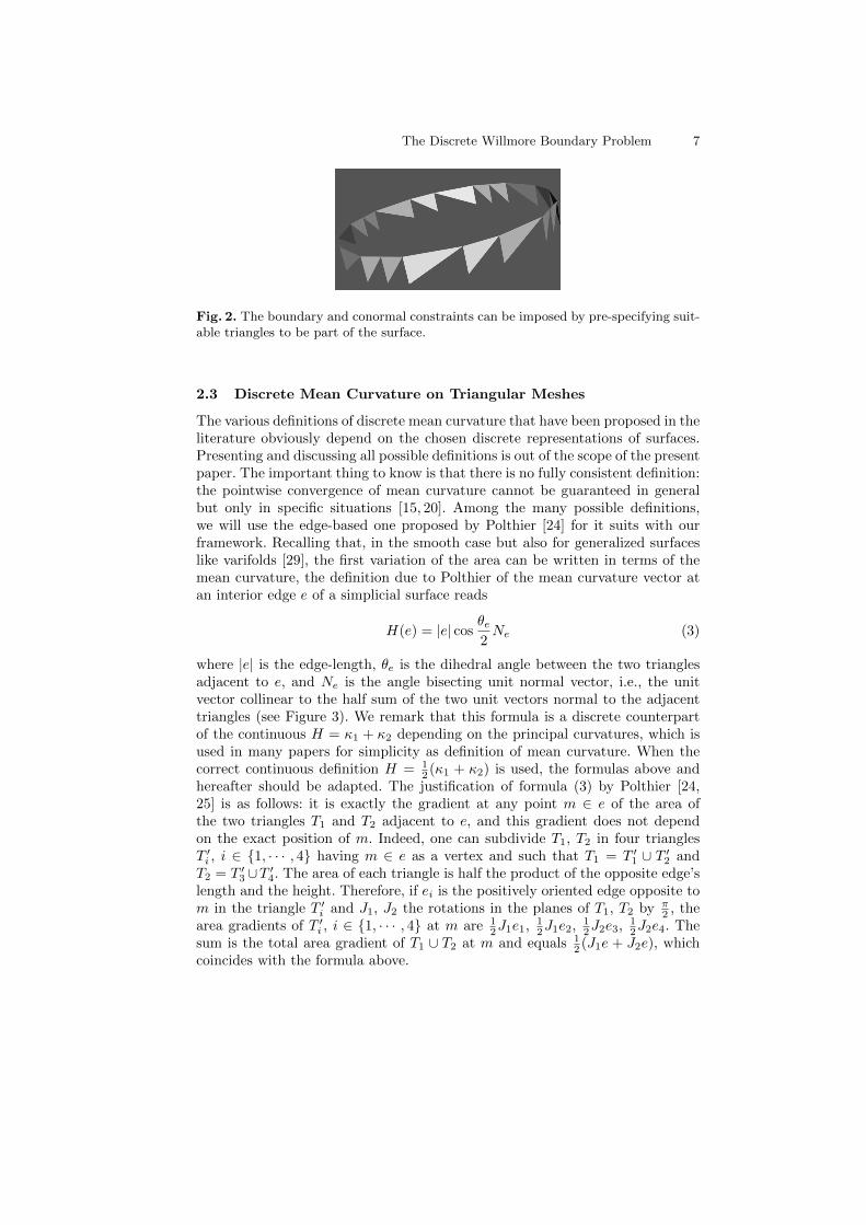
The various definitions of discrete mean curvature that have been proposed in theliterature obviously depend on the chosen discrete representations of surfaces.Presenting and discussing all possible definitions is out of the scope of the presentpaper. The important thing to know is that there is no fully consistent definition:the pointwise convergence of mean curvature cannot be guaranteed in generalbut only in specific situations [15, 20]. Among the many possible definitions,we will use the edge-based one proposed by Polthier [24] for it suits with ourframework. Recalling that, in the smooth case but also for generalized surfaceslike varifolds [29], the first variation of the area can be written in terms of themean curvature, the definition due to Polthier of the mean curvature vector atan interior edge e of a simplicial surface reads

H(e) = |e| cosθe2Ne (3)

where |e| is the edge-length, θe is the dihedral angle between the two trianglesadjacent to e, and Ne is the angle bisecting unit normal vector, i.e., the unitvector collinear to the half sum of the two unit vectors normal to the adjacenttriangles (see Figure 3). We remark that this formula is a discrete counterpartof the continuous H = κ1 + κ2 depending on the principal curvatures, which isused in many papers for simplicity as definition of mean curvature. When thecorrect continuous definition H = 1

2 (κ1 + κ2) is used, the formulas above andhereafter should be adapted. The justification of formula (3) by Polthier [24,25] is as follows: it is exactly the gradient at any point m ∈ e of the area ofthe two triangles T1 and T2 adjacent to e, and this gradient does not dependon the exact position of m. Indeed, one can subdivide T1, T2 in four trianglesT ′i , i ∈ {1, · · · , 4} having m ∈ e as a vertex and such that T1 = T ′1 ∪ T ′2 andT2 = T ′3∪T ′4. The area of each triangle is half the product of the opposite edge’slength and the height. Therefore, if ei is the positively oriented edge opposite tom in the triangle T ′i and J1, J2 the rotations in the planes of T1, T2 by π

2 , thearea gradients of T ′i , i ∈ {1, · · · , 4} at m are 1

2J1e1, 12J1e2, 1

2J2e3, 12J2e4. The

sum is the total area gradient of T1 ∪ T2 at m and equals 12 (J1e + J2e), which

coincides with the formula above.


θe

Ne

e

Fig. 3. The edge-based definition of a discrete mean curvature vector due to Polth-ier [24] depends on the dihedral angle θe and the angle bisecting unit normal vectorNe.

As discussed by Wardetsky et al. using the Galerkin theory of approximation,this discrete mean curvature is an integrated quantity: it scales as λ when eachspace dimension is rescaled by λ. A pointwise discrete mean curvature rescalingas 1

λ is given by (see [34])

Hpw(e) =3|e|Ae

cosθe2Ne,

where Ae denotes the total area of the two triangles adjacent to e. The factor3 comes from the fact that, when the mean curvatures are summed up over alledges, the area of each triangle is counted three times, once for each edge. Then

a discrete counterpart of the energy

∫Σ

ϕ(H) dA is given by

∑edges e

Ae3ϕ(

3|e|Ae

cosθe2Ne). (4)

In particular, the edge-based total squared mean curvature is∑edges e

3|e|2

Ae(cos

θe2

)2. (5)

3 A Quadratic Program for the Minimization of theDiscrete willmore Energy

Ultimately we are aiming at casting the optimization problem in a form that canbe handled by standard linear optimization software. Having in mind the frame-work described above where a discrete surface spanning the prescribed discreteboundary is given as a collection of oriented triangles satisfying equation (2) andchosen among a pre-specified collection of triangles, a somewhat natural direc-tion at first glance seems to be solving a quadratic program. Like in Section 2.1,let us indeed denote as (xi) the collection of binary variables associated to the“dictionary” of triangles (Ti) and define

– eij the common edge to two adjacent triangles Ti and Tj ;


– θij the corresponding dihedral angle;– Nij the angle bisecting unit normal;– Aij the total area of both triangles.

Then a continuous energy of the form

∫Σ

ϕ(x, n,H)dA can be discretized as

∑i,j

qij xi xj (6)

with qij =

1

2

Aij3ϕ(eij , Nij ,

3|eij |Aij

cosθij2Nij) if i 6= j are adjacent

ϕ(Ti, Ni) if i = j

0 otherwise,where ϕ allows to incorporate dependences on each triangle Ti’s position andunit normal Ni. In particular, the discrete Willmore energy is∑

i,j

qwijxi xj (7)

with

qwij =

3|eij |2

2Aij(cos

θij2

)2 if i 6= j are adjacent

0 otherwise.

Assuming that the maps ϕ and ϕ are positive-valued, both energy matrices

Q = (qij) and Qw = (qwij) are symmetric matrices in R+N×N , and the minimiza-tion of either (6) or (7) with boundary constraints turns out to be the followingquadratic program with linear and integrality constraints:

minx

〈Qx, x〉

such that B x = r

xi = 1 ∀i ∈ Jx ∈ {0, 1}N .

We know of no solution to solve this problem efficiently due to the integralityconstraint. What is worse, even the relaxed problem where one optimizes overx ∈ [0, 1]N is very hard to solve: terms of the form xixj with i 6= j are indefinite,so (unless Q has a dominant diagonal) the objective function is a non-convexone.

Moreover, a solution to the relaxed problem would not be of practical use:already for the 2D-problem of optimizing curvature energies over curves in theplane, the respective quadratic program favors fractional solutions. The relax-ation would therefore not be useful for solving the integer program. However, inthis case Amini et al. [3] showed that one can solve a linear program instead.This inspired us for the major contribution of this work: to cast the problem asan integer linear program.


4 An Integer Linear Programming Approach

4.1 Augmented Indicator Vectors

The key idea of the proposed integer linear program is to consider additionalindicator vectors. Aside from the indicator variables xi for basic triangles, onenow also considers entries xij corresponding to pairs of adjacent triangles 4. Sucha pair is called quadrangle in the following. We will denote x the augmentedvector (x1, · · · , xN , · · · , xij , · · · ) where i 6= j run over all indices of adjacenttriangles. The cost function can be easily written in a linear form with thisaugmented vector, i.e. it reads ∑

wkxk

with (see the notations of the previous section)

wk =

{qii if xk = xiqij if xk = xij .

The major problem to overcome is how to set up a system of constraints thatguarantees consistency of the augmented vector: the indicator variable xij forthe pair of triangles i and j should be 1 if and only if both the variables xi andxj are 1. Otherwise it should be 0. In addition, one again wants to optimize onlyover indicator vectors that correspond to a triangular mesh.

To encode this in a linear constraint system, a couple of changes are necessary.First of all, we will now have a constraint for each pair of triangle and adjacentedge. Secondly, edges are no longer oriented. Still, the set of pre-specified indicesJ implies that the orientation of the border is fixed - we still require that foreach edge of the boundary an adjacent (oriented) triangle is fixed to constrainthe conormal information.

To encode the constraint system we introduce a modified notion of incidence.We are no longer interested in incidence of triangles and edges. Instead we nowconsider the incidence of both triangles and quadrangles to pairs of triangles and(adjacent) edges.

For convenience, we define that triangles are positive incident to a pair ofedge and triangle, whereas all quadrangles are negative incident.

We propose an incidence matrix where lines correspond to pairs (triangle,edge) and columns to either triangles or quadrangles. The entries of this incidencematrix are either the incidence of a pair (triangle, edge) with a triangle, definedas

d((triangle k, edge e), triangle i) =

{1 if i = k, e is an edge of triangle i

0 otherwise,

4 This strategy of doubling the variables shares some similarity with techniques insemi-definite programming


or the incidence of a pair (triangle, edge) with a quadrangle, defined as

d((triangle k, edge e), quadrangle ij) =

{−1 if i=k or j=k and i, j share e

0 otherwise.

The columns of this incidence matrix are of two types: either with only 0’s andexactly three 1 (a column corresponding to a triangle T , whose three edges arefound at lines (T, e1), (T, e2), (T, e3)), or with only 0’s and exactly two (−1)’s (acolumn corresponding to a quadrangle (T1, T2) that matches with lines (T1, e12)and (T2, e12)).

Again, both the conormal constraints and the boundary edges can be imposedby imposing additional triangles indexed by a collection J of indices. The generalconstraint has the form∑

i

d((xk, e), xi) +∑i,j

d((xk, e), xij) = r′(k,e),

where the right-hand side depends whether the edge e is shared by two trianglesof the surface (and even several quadrangles in case of self-intersection), or be-longs to the new boundary indicated by the additional triangles. If e is an inneredge, then the sum must be zero due to our definition of d, otherwise there isan adjacent triangle, but no adjacent quadrangle, so the right-hand side shouldbe 1:

r′(k,e) =

{1 if k ∈ J , e is part of the modified boundary

0 otherwise.

To sum up, we get the following integer linear program:

minx

〈w, x〉 (8)

such that D x = r′

xj = 1 ∀j ∈ Jxi ∈ {0, 1} ∀i ∈ {1, . . . , N}

where N is the total number of entries in x, namely all triangles plus all pairsof adjacent triangles. It is worth noticing that such formulation allows trianglesurfaces with self-intersection.

4.2 On the Linear Programming Relaxation

Solving integer linear programs is an NP-complete problem, see e.g. [28, Chapter18.1]. This implies that, to the noticeable exception of a few particular prob-lems [28], no efficient solutions are known. As a consequence one often resortsto solving the corresponding linear programming (LP) relaxation, i.e. one drops


the integrality constraints. In our case this means to solve the problem:

minx

〈w, x〉 (9)

such that D x = r′

xj = 1 ∀j ∈ J0 ≤ xi ≤ 1 ∀i ∈ {1, . . . , N}

or, equivalently, by suitably augmenting D and r′ in order to incorporate thesecond constraint xj = 1, ∀j ∈ J :

minx〈w, x〉 such that Dx = r

0 ≤ xi ≤ 1 ∀i ∈ {1, . . . , N}(10)

There are various algorithms for solving this problem, the most classical beingthe simplex algorithm and several interior point algorithms. Let us now discussthe conditions under which these relaxed solutions are also solutions of the orig-inal integer linear program. Recalling the basics of LP-relaxation [28], the set ofadmissible solutions

P = {x ∈ RN , Dx = r, 0 ≤ x ≤ 1}

is a polyhedron, i.e. a finite intersection of half-spaces in RN . A classical resultstates that minimizing solutions for the linear objective functions can be soughtamong the extremal points of P only, i.e. its vertices. Denoting Pe the integral

envelope of P , that is the convex envelope of P ∩ ZN , another classical resultstates that P has integral vertices only (i.e. vertices with integral coordinates)if and only if P = Pe

Since P = {x ∈ RN , Dx = r, 0 ≤ x ≤ 1}, according to Theorem 19.3 in [28],a sufficient condition for having P = Pe is the property of B being totallyunimodular, i.e. any square submatrix has determinant either 0, −1 or 1. Underthis condition, any extremal point of P that is a solution of

minDx=r, xi∈[0,1]

〈w, x〉

has integral coordinates therefore is a solution of the original integer linear pro-gram

minDx=r, xi∈{0,1}

〈w, x〉.

Theorem 19.3 in [28] mentions an interesting characterization of total unimodu-larity due to Paul Camion [7]: a matrix is totally unimodular if, and only if, thesum of the entries of every Eulerian square submatrix (i.e. with even rows andcolumns) is divisible by four.

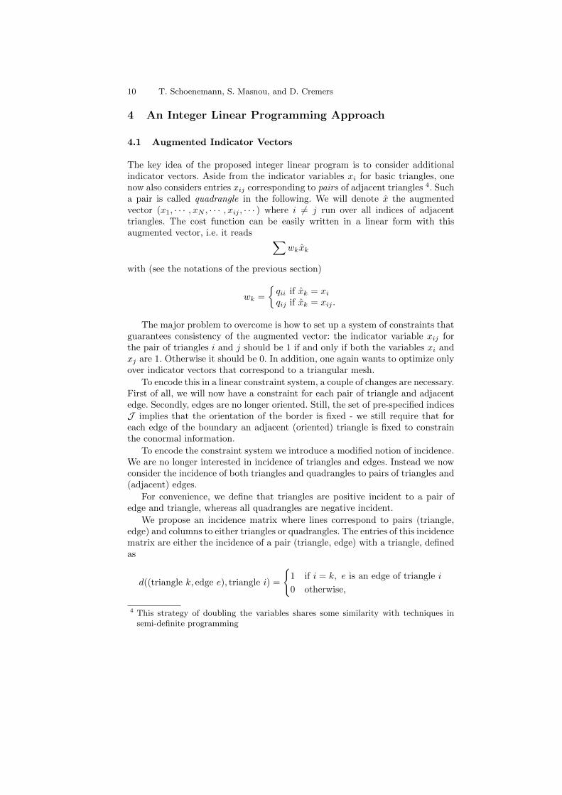
Unfortunately, we can prove that, as soon as the triangle space is rich enough,the incidence matrix D does not satisfy Camion’s criterion, therefore is nottotally unimodular, and neither are the matrices for richer triangles spaces. As


... 24T

T9

T2 T1e2

e

e3

1

T

T ...T10 13

3 T T T T4 6 7

5

8

T

T14

Fig. 4. A configuration in a tri-angle space with sufficient reso-lution. The associated incidencematrix is Eulerian (see text)but does not satisfy Camion’scriterion, thus is not totallyunimodular.

a consequence, there are choices of the triangle space for which the polyhedron

P = {x ∈ RN , Dx = r, 0 ≤ x ≤ 1} may have not only integral vertices, or moreprecisely one cannot guarantee this property thanks to total unimodularity. Thisis summarized in the following theorem.

Theorem 1. The incidence matrix associated with any triangle space whereeach triangle has a large enough number of adjacent neighbors is not totallyunimodular.

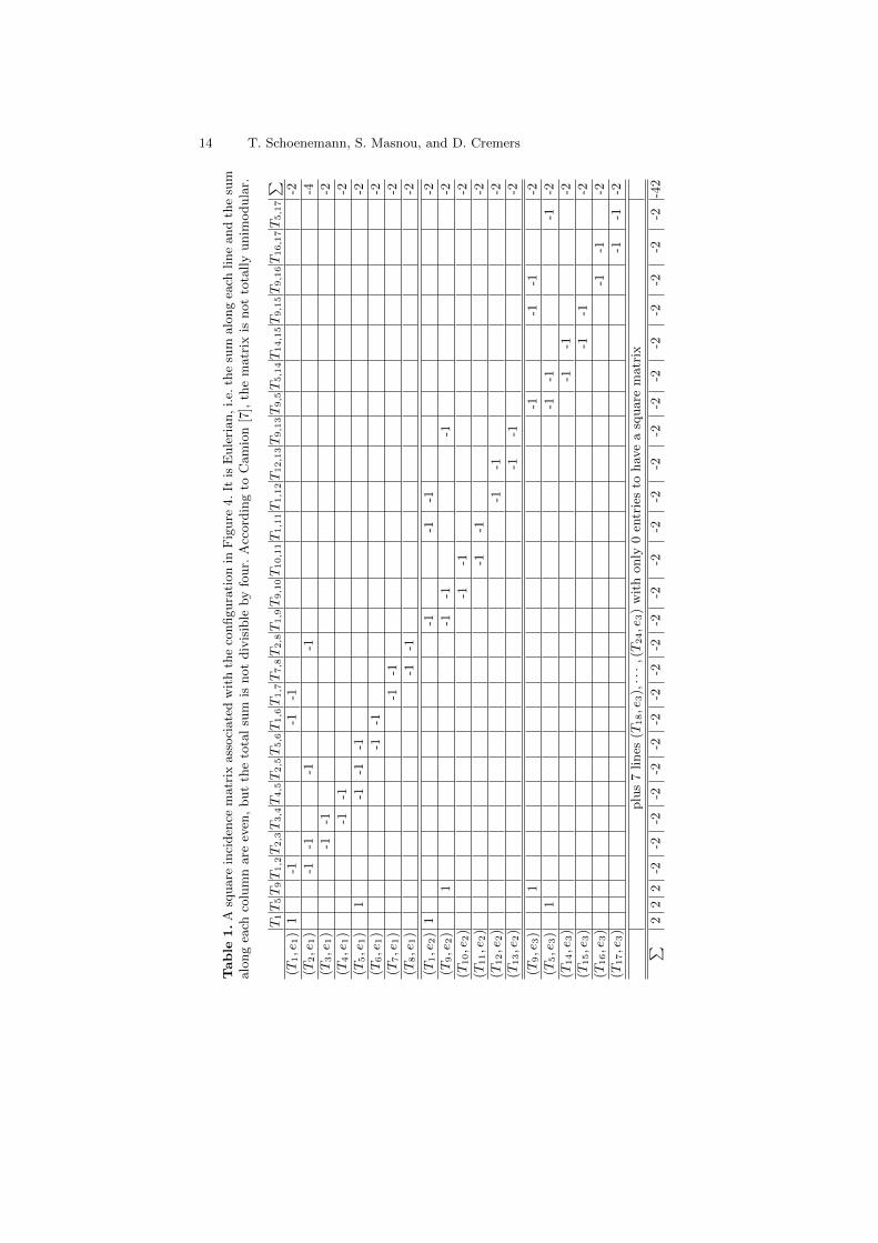
Proof. We show in Figure 4 a configuration and, in Table 1, an associated squaresubmatrix of the incidence matrix. The sum of entries over each line and thesum over each column are even, though the total sum of the matrix entries isnot divisible by four. By a result of Camion [7], the incidence matrix is nottotally unimodular which yields the conclusion according to Theorem 19.3 in[28]. Clearly, any triangle space for which this configuration can occur is alsoassociated to an incidence matrix that is not totally unimodular. �

It is worth noticing that the previous theorem does not imply that the extremalpoints of the polyhedron P are necessarily not all integral. It only states thatthis cannot be guaranteed as usual by the criterion of total unimodularity.

For the sake of completeness, let us mention that there actually exist neces-sary and sufficient conditions of integrality due to Truemper [32], or sufficientconditions different from above due to Grady [13], but we have not been able toexploit them so far.

We will discuss in the next section what additional informations about inte-grality can be obtained from a few experiments that we have done using classicalsolvers for addressing the relaxed linear problem.


Table

1.

Asq

uare

inci

den

cem

atr

ixass

oci

ate

dw

ith

the

configura

tion

inF

igure

4.

Itis

Eule

rian,

i.e.

the

sum

alo

ng

each

line

and

the

sum

alo

ng

each

colu

mn

are

even

,but

the

tota

lsu

mis

not

div

isib

leby

four.

Acc

ord

ing

toC

am

ion

[7],

the

matr

ixis

not

tota

lly

unim

odula

r.

T1T5T9T1,2T2,3T3,4T4,5T2,5T5,6T1,6T1,7T7,8T2,8T1,9T9,10T10,11T1,11T1,12T12,13T9,13T9,5T5,14T14,15T9,15T9,16T16,17T5,17

∑(T

1,e

1)

1-1

-1-1

-2

(T2,e

1)

-1-1

-1-1

-4

(T3,e

1)

-1-1

-2

(T4,e

1)

-1-1

-2

(T5,e

1)

1-1

-1-1

-2

(T6,e

1)

-1-1

-2

(T7,e

1)

-1-1

-2

(T8,e

1)

-1-1

-2

(T1,e

2)

1-1

-1-1

-2

(T9,e

2)

1-1

-1-1

-2

(T10,e

2)

-1-1

-2

(T11,e

2)

-1-1

-2

(T12,e

2)

-1-1

-2

(T13,e

2)

-1-1

-2

(T9,e

3)

1-1

-1-1

-2

(T5,e

3)

1-1

-1-1

-2

(T14,e

3)

-1-1

-2

(T15,e

3)

-1-1

-2

(T16,e

3)

-1-1

-2

(T17,e

3)

-1-1

-2

plu

s7

lines

(T18,e

3),···,

(T24,e

3)

wit

honly

0en

trie

sto

hav

ea

square

matr

ix∑

22

2-2

-2-2

-2-2

-2-2

-2-2

-2-2

-2-2

-2-2

-2-2

-2-2

-2-2

-2-2

-2-4

2


4.3 Testing the Relaxed Linear Problem

We have tested the relaxed formulation on a few examples at low-resolutionusing the dual simplex method implemented in the CLP solver. The main reasonfor using low-resolution is that the number of triangles becomes significantlyimportant as the resolution increases, and both the computational cost andthe memory requirements tend to become large. Another reason for workingat low-resolution is that there is no need to go high before finding a case ofnon-integrality. Indeed, consider the examples in Figure 5: integral solutions areobtained when the resolution is very low (i.e. when there is no risk to haveconfigurations like in Figure 4). In the last configuration, however, the optimalsolution of the relaxed problem has fractional entries. This confirms that ourinitial problem cannot be addressed though the classical techniques of relaxation,and with usual LP solvers.

4.4 On Integer Linear Programming

Our results above indicate that, necessarily, integer linear solvers [28, 1] shouldbe used. These commonly start with solving the linear programming relaxations,then derive further valid inequalities (called cuts) and/or apply a branch-and-bound scheme. Due to the small number of fractional values that we have ob-served in our experiments, it is quite likely that the derivation of a few cuts onlywould give integral solutions. However, we did not test this so far because ofthe running times of this approach: in cases where we get fractional solutionsthe dual simplex method often needs as long as two weeks and up to 12 GBmemory! From experience with other linear programming problems we considerit likely that the interior point methods implemented in commercial solvers willbe much faster here (we expect less than a day). At the same time, we expectthe memory consumption to be considerably higher, so the method would mostprobably be unusable in practice.

We strongly believe that a specific integer linear solver should be developedrather than using general implementations. It is well known that, for a few prob-lems like the knapsack problem, see Chapter 24.6 of [28], their specific structuregives rise to ad-hoc efficient approaches. Recalling that our incidence matrix isvery sparse and well structured (the nonzero entries of each column are eitherexactly two (−1), or exactly three 1) we strongly believe that an efficient integersolver can be developed and our approach can be amenable to higher-resolutionresults in the near future.

5 Conclusion

We have shown that the minimization under boundary constraints of mean cur-vature based energies over surfaces, and in particular the Willmore energy, canbe cast as an integer linear program. Unfortunately, this integer program isnot equivalent to its relaxation so the classical LP algorithms offer no warranty


Fig. 5. A series of experiments (the result and the mesh edges) with increasing resolu-tion of the triangle space (and various boundary constraints). An integral solution ofthe relaxed problem is obtained by a standard LP-solver in both top cases. As for thelast case, the triangle space resolution is now large enough for having configurationssimilar to the counterexample of figure 4. And indeed, an optimal solution is found forthe relaxed problem that is not integral. The mesh on the bottom-right shows actuallytwo nested semi-spheres whose triangles have, at least for a few of them, non binarylabels.


that the integer optimal solution will be found. This implies that pure integerlinear algorithms must be used, which are in general much more involved. Webelieve however that the particular structure of the problem paves the way to adedicated algorithm that would provide high-resolution global minimizers of theWillmore boundary problem and generalizations. This is the purpose of futureresearch.

References

1. T. Achterberg. Constraint Integer Programming. PhD thesis, Technische UniversitatBerlin, 2007.

2. F. Almgren, J.E. Taylor, and L.-H. Wang. Curvature-driven flows: a variationalapproach. SIAM Journal on Control and Optimization, 3:387–438, 1993.

3. A.A. Amini, T.E. Weymouth, and R.C. Jain. Using dynamic programming forsolving variational problems in vision. IEEE Trans. on Patt. Anal. and Mach.Intell., 12(9):855 – 867, September 1990.

4. A.I. Bobenko and P. Schroder. Discrete Willmore Flow. In Eurographics Symposiumon Geometry Processing, 2005.

5. Y. Boykov and V. Kolmogorov. An experimental comparison of min-cut/max-flowalgorithms for energy minimization in computer vision. In A.K. Jain M. Figueiredo,J. Zerubia, editor, Int. Workshop on Energy Minimization Methods in ComputerVision and Pattern Recognition (EMMCVPR), volume 2134 of LNCS, pages 359–374. Springer Verlag, 2001.

6. K.A. Brakke. The surface evolver. Experimental Mathematics, 1(2):141–165, 1992.7. P. Camion. Characterization of totally unimodular matrices. Proc. Am. Math. Soc.,

16(5):1068–1073, 1965.8. U. Clarenz, U. Diewald, G. Dziuk, M. Rumpf, and R. Rusu. A finite element

method for surface restoration with smooth boundary conditions. Computer AidedGeometric Design, 21(5):427–445, 2004.

9. M. Droske and M. Rumpf. A level set formulation for Willmore flow. Interfaces andFree Boundaries, 6(3), 2004.

10. G. Dziuk. Computational parametric Willmore flow. Numer. Math., 111:55–80,2008.

11. S. Esedoglu, S. Ruuth, and R.Y. Tsai. Threshold dynamics for high order geometricmotions. Technical report, UCLA CAM report, 2006.

12. L.R. Ford and D. Fulkerson. Flows in Networks. Princeton University Press,Princeton, New Jersey, 1962.

13. L. Grady. Minimal surfaces extend shortest path segmentation methods to 3D.IEEE Trans. on Patt. Anal. and Mach. Intell. vol 32(2): 321-334, Feb. 2010.

14. R. Grzibovskis and A. Heintz. A convolution-thresholding scheme for the Willmoreflow. Technical Report Preprint 34, Chalmers University of Technology, Goteborg,Sweden, 2003.

15. K. Hildebrandt, K. Polthier, and M. Wardetzky. On the convergence of metricand geometric properties of polyhedral surfaces. Geometriae Dedicata, 123:89–112,2005.

16. L. Hsu, R. Kusner, and J. Sullivan. Minimizing the squared mean curvature integralfor surfaces in space forms. Experimental Mathematics, 1(3):191–207, 1992.

17. R. Kusner. Comparison surfaces for the Willmore problem. Pacific J. Math.,138(2), 1989.


18. S. Luckhaus and T. Sturzenhecker. Implicit time discretization for the meancurvature flow equation. Calculus of variations and partial differential equations,3(2):253–271, 1995.

19. U.F. Mayer and G. Simonett. A numerical scheme for axisymmetric solutions ofcurvature-driven free boundary problems, with applications to the willmore flow.Interfaces and Free Boundaries, 4:89–109, 2002.

20. J.-M. Morvan. Generalized Curvatures. Springer Publishing Company, Incorpo-rated, 1 edition, 2008.

21. N. Olischlager and M. Rumpf. Two step time discretization of willmore flow. InProc. 13th IMA Int. Conf. on Math. of Surfaces, pages 278–292, Berlin, Heidelberg,2009. Springer-Verlag.

22. U. Pinkall. Hopf tori in S3. Invent. Math., 81:379–386, 1985.23. U. Pinkall and I. Sterling. Willmore surfaces. The Mathematical Intelligencer, 9(2),

1987.24. K. Polthier. Polyhedral surfaces of constant mean curvature. Habilitation thesis,

TU Berlin, 2002.25. K. Polthier. Computational aspects of discrete minimal surfaces. In Global Theory

of Minimal Surfaces, Proc. of the Clay Mathematics Institute Summer School, 2005.26. R. Rusu. An algorithm for the elastic flow of surfaces. Interfaces and Free Bound-

aries, 7:229–239, 2005.27. R. Schatzle. The Willmore boundary problem. Calc. Var. Part. Diff. Equ., 37:275–

302, 2010.28. A. Schrijver. Theory of linear and integer programming. Wiley-Interscience series

in discrete mathematics. John Wiley and Sons, July 1994.29. L. Simon. Lectures on Geometric Measure Theory, volume 3 of Proc. of the Center

for Mathematical Analysis. Australian National University, 1983.30. J.M. Sullivan. A Crystalline Approximation Theorem for Hypersurfaces. PhD

thesis, Princeton University, Princeton, New Jersey, 1992.31. J.M. Sullivan. Computing hypersurfaces which minimize surface energy plus bulk

energy. Motion by Mean Curvature and Related Topics, pages 186–197, 1994.32. K. Truemper, Algebraic Characterizations of Unimodular Matrices. SIAM J.

Applied Math., vol. 35(2): 328-332, Sept. 1978.33. J. Verdera, V. Caselles, M. Bertalmio, and G. Sapiro. Inpainting surface holes. In

In Int. Conference on Image Processing, pages 903–906, 2003.34. M. Wardetzky, M. Bergou, D. Harmon, D. Zorin, and E. Grinspun. Discrete

quadratic curvature energies. Computer Aided Geometric Design, 24(8–9):499–518,2007.

Documents

On a Linear Programming Approach to the Discrete …math.univ-lyon1.fr/~masnou/fichiers/publications/avignon.pdfnonlinear boundary value problem into an integer linear ... integer